Holographic estimate of the meson cloud contribution to nucleon axial form factor

Abstract

We use light-front Holography to estimate the valence quark and the meson cloud contributions to the nucleon axial form factor. The free couplings of the holographic model are determined by the empirical data and by the information extracted from lattice QCD. The holographic model provides a good description of the empirical data when we consider a meson cloud mixture of about 30% in the physical nucleon state. The estimate of the valence quark contribution to the nucleon axial form factor compares well with the lattice QCD data for small pion masses. Our estimate of the meson cloud contribution to the nucleon axial form factor has a slower falloff with the square momentum transfer compared to typical estimates from quark models with meson cloud dressing.

I Introduction

In recent years, it was found that the combination of the 5D gravitational anti-de Sitter (AdS) space and conformal field theories (CFT) can be used to study QCD in the confining regime Maldacena99 ; Witten98 ; Gubser98 ; Brodsky15 . Using this formalism one can relate the results from AdS/CFT with the results from light-front dynamics based on a Hamiltonian that include the confining mechanism of QCD (AdS/QCD) Brodsky15 . In the limit of massless quarks, one can relate the AdS holographic variable $z$ with the impact separation $\zeta$, which measures the distance of constituent partons inside the hadrons Brodsky15 ; Brodsky08a ; Teramond09a . This correspondence (duality) between the two formalisms is known as light-front holography or holographic QCD.

Over the last few years light-front holography has been used to study several proprieties of the hadrons. The soft-wall formulation of the light-front holography introduces a holographic mass scale $\kappa$, which is fundamental for the description of the hadron spectrum (mesons and baryons) and hadron wave functions Brodsky15 ; Karch06 ; Grigoryan07a ; Branz10a ; Gutsche12b ; Teramond15a . This scale can be estimated from the holographic expression for the $\rho$ mass $m_{\rho}\simeq 2\kappa$ Brodsky15 ; Grigoryan07a . Examples of applications of light-front holography are in the calculation of parton distribution functions, hadron structure form factors among others Brodsky15 ; Brodsky08a ; Chakrabarti13a ; Abidin09 ; Teramond11a ; Liu15c ; Sufian17a ; Gutsche13a ; Gutsche12a ; RoperHol ; RoperAn ; Vega11 ; Chakrabarti13 .

In the light-front formalism one can represent the wave functions of the hadrons using an expansion of Fock states with a well defined number of partons Brodsky15 . In the case of baryons, the first term corresponds to the three-quark state ($qqq$). The following terms are excitations associated with a gluon, $(qqq)g$, with a quark-antiquark pair, $(qqq)q\bar{q}$, and higher order terms. Those states can be labeled in terms of the number of partons $\tau=3,4,5,...$, respectively. The calculation of structure form factors between baryon states can then be performed using the light-front wave functions and the interaction vertices associated with the respective transition Abidin09 ; Gutsche12a ; RoperHol . The form factors can also be expanded in contributions from the valence quarks and in contributions from the meson cloud Brodsky15 ; Gutsche12a ; Gutsche13a . Examples of calculations of the nucleon and the nucleon to Roper electromagnetic form factors can be found in Refs. Gutsche12a ; RoperHol ; RoperAn ; Brodsky15 ; Teramond11a ; Abidin09 ; Chakrabarti13a ; Liu15c ; Sufian17a ; Gutsche13a .

In principle the leading twist approximation, associated with the three-quark state, is sufficient to explain the dominant contribution of the form factors related to the electromagnetic transitions between baryon states, particularly at large momentum transfer. In the case of the nucleon and the Roper, the electromagnetic form factors can be described in a good approximation by the valence quark effects (leading twist approximation) Brodsky15 ; RoperHol ; Chakrabarti13a ; Liu15c . There is, however a rising interest in checking if the holography can be used to estimate higher order corrections to the transition form factors, particularly, in the corrections associated with the meson cloud excitations, related in the light-front formalism to the state $(qqq)q\bar{q}$, of order $\tau=5$ Gutsche12a ; Gutsche13a ; Sufian17a .

The question of whether the light-front meson cloud contribution is important or not is pertinent, because in principle the corrections associated with the meson cloud should be expressed in terms of parameters related to the microscopic structure, such as meson-baryon couplings and the photon-meson couplings NucleonMC1 ; NucleonMC2 ; NucleonMC3 . As discussed later, in the case of a holographic model, the estimates of the transition form factors depend only on the couplings associated with quarks without explicit reference to the substructure associated with the meson cloud.

In this work we study the axial structure of the nucleon using a holographic model based on a soft-wall confining potential. The weak structure of the nucleon is characterized by the axial form factor, $G_{A}$, and the induced pseudoscalar form factor, $G_{P}$. The study of the nucleon axial structure is important because it provides complementary information on the well known electromagnetic structure and also because involves both strong and weak interactions AxialFF . The nucleon axial form factors can be measured in quasi-elastic neutrino/antineutrino scattering with proton targets, by charged pion electroproduction on nucleons and also in the process of muon capture by protons Bernard02 ; Schindler07a ; Gorringe05 . The value of the axial form factor at $Q^{2}=0$ is determined with great accuracy by neutron $\beta$ decay Bernard02 ; PDG2014 .

The nucleon axial form factor has been calculated using different frameworks AxialFF ; NSTAR ; Gaillard84 ; JDiaz04 ; Adamuscin08 ; Thomas84 ; Tsushima88 ; Shanahan13 ; Schlumpf93a ; Boffi02 ; Merten02 ; BCano03 ; Silva05 ; Pasquini07 ; Anikin16a ; Dahiya14a ; Liu15a ; Liu16a ; Eichmann12 ; Chang13 ; Yamanaka14 ; Mamedov16a . Recently, also lattice QCD simulations of the nucleon axial form factors became available for several pion masses ($m_{\pi}$), in the range $m_{\pi}=0.2$–0.6 GeV Sasaki03 ; Edwards06 ; Yamazaki08 ; Bhattacharya14 ; Sasaki08 ; Yamazaki09 ; Bratt10 ; Alexandrou13 ; Alexandrou11a ; Horsley14 ; ARehim15 ; Bali15 ; Bhattacharya16 ; Green17 ; Capitani17 ; Liang16 ; Berkowitz17 ; Yao17 .

In the present work our goal is to study the role of the valence quarks (leading twist approximation) and the role of the meson cloud ($\tau=5$) in the nucleon axial form factor $G_{A}$. We consider in particular the holographic model from Ref. Gutsche12a , neglecting the gluon effects. We assume that the gluon effects are included effectively in the quark structure through the gluon dressing. In that case the next leading order correction is associated with the quark-antiquark excitations of the three valence quark core. In this context the bare and the meson cloud contribution to the nucleon axial form factor are both expressed in terms of two independent parameters: $g_{A}^{0}$ and $\eta_{A}$, associated with the quark axial and quark induced pseudoscalar couplings Gutsche12a .

To calculate the contributions associated with the nucleon bare core and the meson cloud we use the available experimental data and the results from lattice QCD, which help to constrain the contributions from the pure valence quark degrees of freedom, and therefore fix also the contributions of the meson cloud component. In the lattice QCD simulations with large pion masses the meson cloud effects are very small, and the physics associated with the valence quarks can be better calibrated.

The results from lattice QCD cannot be directly related to the valence quark contributions to the axial form factor, because the lattice calculations are not performed at the physical limit (physical quark masses). The results from lattice can, however, be extrapolated to the physical case with the assistance of quark models that include a dynamic dependence on the quark mass.

Once fixed the parameters of the holographic model by the empirical and lattice QCD data, the holographic model can be used to estimate the fraction of the meson cloud contribution to the nucleon axial form factor. This estimate can be compared to other estimates from quark models with meson cloud dressing.

We conclude at the end that the holographic model considered in the present work describes accurately the experimental data for the nucleon axial form factor, and that the lattice QCD data with small pion masses can be well approximated by the estimate of the valence quark contributions, in all ranges of $Q^{2}$. We also conclude that the meson cloud contribution falls off very slowly with the square momentum transfer $Q^{2}$, much slower than estimates based on quark models.

This article is organized as follows. In Sec. II, we discuss the formalism associated with the study of the axial structure of the nucleon, including the axial current, parametrizations of the data, results from lattice QCD, as well as theoretical models based on a valence quark core with meson cloud dressing. In Sec. III, we present the holographic model for nucleon axial form factor considered in the present work. The numerical results of the nucleon axial form factor and for the estimate of the meson cloud contributions based on the holographic model appear in Sec. IV. The outlook and the conclusions are presented in Sec. V.

II Background

We now discuss the background associated with the study of the nucleon axial form factor. We start with the representation of the axial current and the definition of the axial form factors. Next, we summarize the experimental status of the nucleon axial form factor $G_{A}$. Later, we explain how the experimental data can be described within a quark model for the bare core, combined with a meson cloud dressing of the core. Finally, we discuss the results from lattice QCD and how those results can be related with the function $G_{A}$ in the physical limit.

II.1 Axial current

The weak-axial transition between two nucleon states with initial momentum $p$, final momentum $p^{\prime}$, and transition momentum $q=p^{\prime}-p$, is characterized by the weak-axial current Bernard02 ; Schindler07a

$$\left(J_{5}^{\mu}\right)_{a}=\bar{u}(p^{\prime})\left[G_{A}(Q^{2})\gamma^{\mu}+G_{P}(Q^{2})\frac{q^{\mu}}{2M}\right]\gamma_{5}u(p)\frac{\tau_{a}}{2},$$

(1)

where $M$ is the nucleon mass, $Q^{2}=-q^{2}$, $\tau_{a}$ ($a=1,2,3$) are Pauli isospin operators and $u(p)$, $u(p^{\prime})$ are the Dirac spinors associated with the initial and final states, respectively. The functions $G_{A}$ and $G_{P}$ define, respectively, the axial-vector and the induced pseudoscalar form factors. In the present work we restrict the analysis to the axial-vector form factor, refereed to hereafter, simply as the axial form factor. The leading order contribution for $G_{P}$ can be estimated considering the meson pole contribution, $G_{P}=\frac{4M^{2}}{m_{\pi}^{2}+Q^{2}}G_{A}$, derived from the partial conservation of the axial current AxialFF ; Bernard02 ; Thomas84 ; Sasaki08 ; Schindler07a ; Gorringe05 .

Using the spherical representation ($a=0,\pm$) we can interpret $(J_{5}^{\mu})_{0}$ as the current associated with the neutral transitions, $p\to p$ and $n\to n$ ($Z^{0}$ production), and the current associated with $a=\pm$ with the $W^{\pm}$ production ($n\to p$ and $p\to n$ transitions).

II.2 Experimental status

The function $G_{A}$ can be measured by neutrino scattering and pion electroproduction off nucleons. Both experiments suggest a dipole dependence $G_{A}(Q^{2})=G_{A}(0)/(1+Q^{2}/M_{A}^{2})^{2}$, where the values of $M_{A}$ vary between 1.03 and 1.07 GeV depending on the method Bernard02 ; Schindler07a .

To represent the experimental data in a general form we consider the interval between the two functions, $G_{A}^{{\rm exp}-}$ and $G_{A}^{{\rm exp}+}$, given by AxialFF

$$G_{A}^{{\rm exp}\pm}(Q^{2})=\frac{G_{A}^{0}(1\pm\delta)}{\left(1+\frac{Q^{2}}{M_{A\pm}^{2}}\right)^{2}},$$ (2)

where $G_{A}^{0}=1.2723$ is the experimental value of $G_{A}(0)$ PDG2014 , $\delta=0.03$ is a parameter that expresses the precision of the data, and $M_{A-}=1.0$ GeV and $M_{A+}=1.1$ GeV are, respectively, the lower and upper limits from $M_{A}$ extracted experimentally. The central value of the parametrization (2) can be approximated by a dipole with $M_{A}\simeq 1.05$ GeV.

Most of the data analysis are restricted to the region $Q^{2}<1$ GeV² Bernard02 . The range of the variation associated with the parametrization of $G_{A}$ represented by Eq. (2) is shown in Fig. 1 by the red band. The short-dashed-line represents the central value of the parametrization.

Recently the nucleon axial form factor was determined in the range $Q^{2}=2$–4 GeV² at CLAS/Jlab Park12 . The new data are consistent with the parametrization (2).

We discuss next, how the axial form factor can be estimated in the context of a quark model with meson cloud dressing of the valence quark core.

II.3 Theory

In a quark model with meson cloud dressing we can represent the physical nucleon state in the form AxialFF

$$\left|N\right>=\sqrt{Z_{N}}\left[\left|3q\right>+b_{N}\left|{\rm MC}\right>\right],$$ (3)

where $\left|3q\right>$ is the three-quark state and $b_{N}\left|{\rm MC}\right>$ is the meson cloud state. The coefficient $b_{N}$ is determined by the normalization $Z_{N}(1+b_{N}^{2})=1$, assuming that $\left|{\rm MC}\right>$ is normalized.

In this representation $Z_{N}=\sqrt{Z_{N}}\sqrt{Z_{N}}$ measures the probability of finding the $qqq$ state in the physical nucleon state. Consequently, $1-Z_{N}$ measures the probability of the meson cloud component in the physical nucleon state.

In Eq. (3), we include only the first correction for the meson cloud, associated with the baryon-meson states. In principle, we should also include corrections associated with baryon-meson-meson states. In the case of the nucleon, however, where the meson cloud is dominated by the pion cloud, the correction of the state $\left|N\pi\right>$ provides a good approximation to the physical nucleon state. In the case of $1-Z_{N}\simeq 0.3$ the correction associated with the two-pion correction is attenuated by the factor $(1-Z_{N})^{2}\simeq 0.09$.

In the calculation of the axial form factors, in order to take into account the contribution of the meson cloud in the form factors at the physical limit, one needs to correct the function $G_{A}^{\rm B}$ by the factor $Z_{N}$, which quantifies the contribution of the bare core to $G_{A}$ AxialFF . The effective contribution from $G_{A}^{\rm B}$ to the physical $G_{A}$ becomes then $Z_{N}G_{A}^{\rm B}$. More generically, we can write

$$G_{A}=Z_{N}G_{A}^{\rm B}+(1-Z_{N})G_{A}^{\rm MC},$$ (4)

where the second term accounts for the contribution from the meson cloud. The function $G_{A}^{\rm MC}$ is the unnormalized meson cloud contribution, estimated when we drop the valence quark contribution.

Hereafter, we use the expression bare contribution to refer the first term of Eq. (4) and meson cloud contribution to refer the second term of Eq. (4).

An alternative representation of the meson cloud term is $(1-Z_{N})G_{A}^{\rm MC}=Z_{N}\tilde{G}_{A}^{\rm MC}$ AxialFF . To convert to $G_{A}^{\rm MC}$, one uses $G_{A}^{\rm MC}=\tilde{G}_{A}^{\rm MC}/(1/Z_{N}-1)$. The function $\tilde{G}_{A}^{\rm MC}$ can be extracted from the data, as discussed in Ref. AxialFF .

II.4 Information from lattice QCD

Another source of information about the axial structure of the nucleon are the lattice QCD simulations. In lattice QCD, one can simulate the dynamic of QCD in a discrete space-time. Since simulations with very small grids and large volumes are very costly, most of the simulations are performed for large values of the pion mass, and the obtained results correspond to quark masses larger than the physical quark masses. For those reasons, some care is necessary in the interpretation of the lattice QCD results, and in the extrapolations, to the continuous limit, to the infinite volume limit, and to the physical limit (physical masses) Bali15 ; Bhattacharya16 .

Nevertheless, lattice QCD can be used to make a connection with results from quark models. In those conditions, lattice QCD can help us to understand the role of the valence quarks in the structure form factors. Since in lattice QCD simulations with large pion masses the effect of the meson cloud dressing is significantly reduced, those simulations can be used to estimate the contribution of the form factors that are the direct consequence of the valence quark effects. Contrary to the lattice QCD calculations of the electromagnetic form factors, the nucleon axial form factor, due to its isovector character, has no contributions associated with the disconnected diagrams in the continuous limit AxialFF ; Alexandrou11a ; Alexandrou13 ; ARehim15 , and can therefore be directly compared to the experimental data.

The axial form factor and the induced pseudoscalar form factor have been calculated in lattice QCD simulations for several values of the pion mass at $Q^{2}=0$ Sasaki03 ; Edwards06 ; Yamazaki08 ; Bhattacharya14 ; Liang16 , and for finite $Q^{2}$ Sasaki08 ; Yamazaki09 ; Bratt10 ; Alexandrou13 ; Alexandrou11a ; Green17 . Simulations with large volumes and pion masses in the range 0.25–0.5 GeV suggest that the values of $G_{A}$ near $Q^{2}=0$ are generally restricted to $G_{A}(0)=1.1$–1.2. Those results indicate that based only on the contributions of the valence quarks it is not possible to reach the experimental value $G_{A}(0)\simeq 1.27$. This underestimation can be inferred as a sign that the meson cloud contribution to $G_{A}$ is positive.

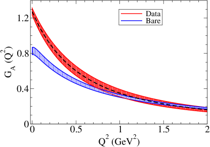
Figure 1: Experimental parametrization of the data $G_{A}^{\rm exp}$ according to Eq. (2), at red, combined with the estimate of the contribution $Z_{N}G_{A}^{\rm B}$ extracted from the lattice QCD data, at blue. The short-dashed-line indicates the central value of Eq. (2).

Estimates of $G_{A}(0)$ near the physical point can be found in Refs. Horsley14 ; ARehim15 ; Bali15 ; Bhattacharya16 ; Capitani17 ; Berkowitz17 ; Yao17 . Lattice QCD simulations with smaller pion masses may include some meson cloud effects and may also be affected by significant finite volume effects, which tend to underestimate the value of $G_{A}(0)$ compared to the infinite volume limit Yamazaki08 ; Yamazaki09 .

The study of the valence quark effects in the nucleon axial form factor can also be performed considering a constituent quark model where the parameters associated with the properties of the quarks are adjusted in order to describe the results from lattice QCD. In this case the decisive parameter is the variable that regulates the quark mass which can be converted into the mass of the pion associated with the lattice QCD regime.

One can then extrapolate the valence quark contribution of $G_{A}$ in the physical limit from the lattice QCD results, using a quark model, if the parameters of the model are defined in terms of the pion mass. It is worth noticing, however, that the function $G_{A}$ extrapolated to the case $m_{\pi}\to m_{\pi}^{\rm phys}$ ($m_{\pi}^{\rm phys}$ represent the physical pion mass), which may be interpreted as $G_{A}^{\rm B}$ (bare contribution), does not represent in fact the bare contribution to the physical form factor. This happens, because in the physical limit, one needs to take into account the effect of the meson cloud dressing and its impact in the physical nucleon wave function, as shown in Eq. (4). The effective contribution to the physical $G_{A}$ is then $Z_{N}G_{A}^{\rm B}$, where $G_{A}^{\rm B}$ is the contribution from the valence quark component, estimated from lattice QCD, and extrapolated to the physical case. An example of a quark model with proprieties mentioned above is the model from Ref. AxialFF .

In Ref. AxialFF , the covariant spectator quark model is applied to the study of the axial structure of the nucleon in the lattice QCD regime, and in the physical regime. In the covariant spectator quark model, hereinafter referred to simply as the spectator model, the nucleon is described as a three valence quark system and the radial wave functions are expressed in terms of momentum scale parameters determined in the study of the nucleon electromagnetic structure Nucleon . The nucleon valence quark wave function is represented by a mixture of two states: the dominant $S$-wave and a small $P$-wave, as in other quark models AxialFF ; Thomas84 . The quark substructure is parametrized by quark electromagnetic and axial form factors, which simulate effectively the internal structure of the constituent quarks, resulting from the interactions with quark-antiquark pairs and from the quark-gluon dressing Nucleon ; Omega1 . The parameters of the spectator model associated with the valence quark structure are first fixed by the lattice QCD data and the results are later extended to the physical limit.

We can summarize the method used in Ref. AxialFF by the following steps:

• Calibration of the parameters associated with the valence quark structure (quark form factors and fraction of $P$-state mixture) using lattice QCD data.

• Extend the result of $G_{A}(Q^{2},m_{\pi})$ to the physical limit ($m_{\pi}\to m_{\pi}^{\rm phys}$) defining the function $G_{A}^{\rm B}(Q^{2})$.

• Use experimental data to determine the factor $Z_{N}$ associated with the normalization of the physical nucleon state, according to

  $$G_{A}^{\rm exp}(Q^{2})\simeq Z_{N}G_{A}^{\rm B}(Q^{2}),$$ (5)

  in the region $Q^{2}>1$ GeV², where the meson cloud effects are expected to be small. This procedure establishes the proportion of meson cloud in the physical nucleon state.

• The contribution from the meson cloud to $G_{A}$ can then be estimated by the difference: $G_{A}^{\rm exp}-Z_{N}G_{A}^{\rm B}$ for small $Q^{2}$ ($Q^{2}<1$ GeV²).

The connection between the spectator model and the lattice regime is performed using wave functions dependent of the mass of the nucleon (physical mass replaced by lattice mass), and quark form factors parametrized in terms of the vector dominance mechanism AxialFF . In the lattice QCD regime, the vector meson physical masses are replaced by the masses of vector mesons in lattice. Except for the masses (baryons and vector mesons) all the parameters of the wave functions and quark form factors are determined by fits to the lattice QCD data. Check Ref. AxialFF for more details about the parametrization of the quark axial structure. More details about the extension of the spectator model to the lattice QCD regime can be found in Refs. Lattice ; LatticeD ; NucleonMC3 ; Octet2 ; Omega1 ; Omega2 .

The function $G_{A}^{\rm B}$ extrapolated from lattice QCD using the spectator model based on the previous procedure is presented in Fig. 1, by the blue band. The $P$-state mixture is 25% AxialFF . The accuracy of the parametrization for $G_{A}^{\rm B}$ is then limited by the precision of the lattice data. Since the lattice data can be very accurate for small $Q^{2}$ ($\sim 1\%$) and have large errorbars for $Q^{2}=2$–4 GeV² ($\sim 10\%$), we consider an average error of 5%.

For future reference, we mention that the parametrization of the meson cloud contribution in the spectator model can be represented by AxialFF

$$G_{A}^{\rm MC}(Q^{2})=\frac{G_{A}^{{\rm MC}0}}{\left(1+\frac{Q^{2}}{\Lambda^{2}}\right)^{4}},$$ (6)

where $G_{A}^{{\rm MC}0}=1.68$ and $\Lambda=1.05$ GeV. Here, $\Lambda$ is the average of the two cutoffs used in the parametrization (2). We recall that the effective contribution of $G_{A}^{\rm MC}$ to $G_{A}$ is the result of the product $(1-Z_{N})G_{A}^{\rm MC}$.

III Holographic Model

Different holographic models have been applied to the systems ruled by QCD. Those models can be classified into two main categories: the bottom-up approach and the top-down approach. The top-down approach is related to supersymmetric strings and it has the base of the $D$-brane physics Nawa07 ; Hong07 ; Hong08 ; Sakai05 ; Hashimoto08 . The bottom-up approach is more phenomenological and derive the QCD proprieties in the confining regime using 5D-fields in AdS space Brodsky15 ; Brodsky08a ; Teramond09a ; Karch06 ; Gutsche12a ; Gutsche13a .

In the present work we consider a bottom-up approach where the confinement is included through a potential $U_{F}(z)$ (soft-wall approximation). We consider in particular the holographic soft-wall model from Ref. Gutsche12a for the nucleon axial form factor.

In holographic QCD the particle fields $\Psi$ and the source fields (electromagnetic and axial) are represented in terms of the coordinates $(x,z)$, where $x$ belongs to the usual 4D space and $z$ is the holographic variable. To describe the structure of the baryons we define fermion fields $\Psi(x,z)$, which encode the proprieties of the baryons. Those fermion fields can be decomposed into different modes $\Psi_{n}$ ($n=0,1,2,...$) which are the holographic analogous of the baryon wave functions Gutsche12a ; Gutsche13a ; Abidin09 .

For the description of the nucleon structure we start by constructing the fermion fields $\Psi_{\pm}(x,z)$ associated with the spin $J=1/2$, where $\pm$ are the left- and right-handed ($L/R$) components of the nucleon radial excitations doublets. The axial structure is introduced by the 5D axial field $\hat{\cal A}_{i}(x,z)$, where $i=\pm$. Following Ref. Gutsche12a , we represent the axial structure in the form

$$\hat{\cal A}_{i}(x,z)=\hat{\cal A}_{i}^{(1)}(x,z)+\hat{\cal A}_{i}^{(2)}(x,z)+\hat{\cal A}_{i}^{(3)}(x,z).$$ (7)

The different terms describe the possible structures associated with the axial interaction in 5D.

The first term is the minimal axial-vector coupling

$$\hat{\cal A}_{i}^{(1)}(x,z)=g_{A}^{0}\Gamma^{M}\gamma_{5}A_{M}(x,z)\frac{\tau_{3}}{2},$$ (8)

where $\Gamma^{M}$ ($M=0,1,2,3,z$) is the 5D gamma matrix, $A_{M}(x,z)$ is the holographic analogous of the axial field and $\tau_{3}=\mbox{diag}(1,-1)$ is the Pauli isospin matrix. The function $A_{M}(x,z)$ is constrained by the gauge condition $A_{z}(x,y)=0$ Gutsche12a . The second term represents a nonminimal coupling, the holographic analogous of the induced pseudoscalar coupling

$$\hat{\cal A}_{i}^{(2)}(x,z)=\eta_{A}\left[\Gamma^{M},\Gamma^{N}\right]\gamma_{5}A_{MN}(x,z)\frac{\tau_{3}}{2},$$ (9)

where $A_{MN}=\partial_{M}A_{N}-\partial_{N}A_{M}$. The final term is an axial-type coupling proportional to the nucleon isovector charge

$$\hat{\cal A}_{i}^{(3)}(x,z)=\mp\Gamma^{M}A_{M}(x,z)\frac{\tau_{3}}{2}.$$ (10)

The fermion fields, mentioned above can be expressed in the Weyl representation in the form

$$\Psi_{\pm,n}(x,z)=z^{2}\left(\begin{array}[]{c}F_{L/R,n}(z)\\ \pm F_{R/L,n}(z)\\ \end{array}\right)\chi_{n}(x),$$ (13)

where $\chi_{n}(x)$ is a two-component spinor and the functions $F_{L/R,n}(z)$ are solutions of Schrödinger-type wave equations in the variable $z$ Gutsche12a ; Gutsche13a ; RoperHol . For simplicity, we omitted the isospin indices. The nucleon case corresponds to the first mode ($n=0$). More details can be found in Refs. Brodsky15 ; Gutsche12a ; Gutsche13a ; Abidin09 .

The axial transition current is calculated considering the overlap of the holographic nucleon fields associated with the initial and final states with the axial field (7). From the axial transition current we can extract the holographic expressions for the axial form factor $G_{A}$ according with the number of constituents.

III.1 Axial form factor

In Ref. Gutsche12a , the contributions associated with the first Fock states are studied in detail, and the effects of the 3, 4 and 5 parton components are calculated explicitly. Those contributions are associated, respectively, with the $qqq$ state (3-quark, index $\tau=3$), the $(qqq)g$ state (3-quark-gluon, index $\tau=4$), and the $(qqq)\bar{q}q$ state (3-quark-quark-antiquark, index $\tau=5$). Neglecting the contributions associated with the gluon states, we can write the nucleon axial form factor $G_{A}$ in the form

$$G_{A}(Q^{2})=c_{3}G_{A}^{\rm B}(Q^{2})+c_{5}G_{A}^{\rm MC}(Q^{2}),$$ (14)

where $G_{A}^{\rm B}$ is the bare contribution associated with the $qqq$ state ($\tau=3$) and $G_{A}^{\rm MC}$ is the meson contribution associated with the $(qqq)q\bar{q}$ state ($\tau=5$). The coefficients $c_{\tau}$ specify the weight of the $\tau$-component of the Fock state, and are in the present approximation restricted to $c_{3}+c_{5}=1$. According to Ref. Gutsche12a , the components $G_{A}^{\rm B}$ and $G_{A}^{\rm MC}$ can be represented in terms of $a=\frac{Q^{2}}{4\kappa^{2}}$, as

$$G_{A}^{\rm B}(Q^{2}) = \left[g_{A}^{0}+\frac{a}{6}(g_{A}^{0}-1)\right]G_{1}$$ (15)

$$+\frac{\eta_{A}}{12}a(2a+17)G_{2},$$

$$G_{A}^{\rm MC}(Q^{2}) = \left[g_{A}^{0}+\frac{a}{10}(g_{A}^{0}-1)\right]G_{3}$$ (16)

$$+\frac{\eta_{A}}{30}a(4a+49)G_{4},$$

where the functions $G_{i}$ ($i=1,2,3,4$) have the following form

$$G_{1} = \frac{1}{\left(1+a\right)\left(1+\frac{a}{2}\right)\left(1+\frac{a}{3}\right)},$$ (17)

$$G_{2} = \frac{1}{\left(1+a\right)\left(1+\frac{a}{2}\right)\left(1+\frac{a}{3}\right)\left(1+\frac{a}{4}\right)},$$ (18)

$$G_{3} = \frac{1}{\left(1+a\right)\left(1+\frac{a}{2}\right)\left(1+\frac{a}{3}\right)\left(1+\frac{a}{4}\right)\left(1+\frac{a}{5}\right)},$$ (19)

$$G_{4} = \frac{1}{\left(1+a\right)\left(1+\frac{a}{2}\right)\left(1+\frac{a}{3}\right)\left(1+\frac{a}{4}\right)\left(1+\frac{a}{5}\right)\left(1+\frac{a}{6}\right)}.$$

Recall that in the previous equations $\kappa$ is the holographic mass scale. In the following, we consider the value $\kappa=0.385$ GeV, in order reproduce approximately the $\rho$ mass ($m_{\rho}\simeq 770$ MeV). The holographic estimate of the nucleon mass is then $2\sqrt{2}\kappa\simeq 1.09$ GeV, a bit above the experimental value.

From Eqs. (15)-(16) we can conclude that at large $Q^{2}$: $G_{A}^{\rm B}\propto 1/Q^{4}$ and $G_{A}^{\rm MC}\propto 1/Q^{8}$. As a consequence, the meson cloud contribution falls off faster than the bare contribution. One can then expect that $G_{A}^{\rm MC}$ become negligible for values of $Q^{2}$ larger than a certain scale. One of the goals of the present study is to estimate that scale.

Concerning the decomposition of the bare and meson cloud contributions in terms of the pole structure of the functions $G_{i}$, some discussion is in order. The present representation in terms of the poles on $a$ is a direct consequence of the calculation of the axial form factors based on the axial coupling (7) and the wave functions (13). The present pole structure of the functions $G_{i}$ is expected for the calculation of the electromagnetic form factors Gutsche12a ; Gutsche13a ; Abidin09 , and can be interpreted in terms of the vector meson dominance (VMD) mechanism Maldacena99 ; Brodsky15 ; Grigoryan07a ; Hong07 ; Hong08 ; Hashimoto08 ; Sakurai60 ; Bauer79 ; Gari84 ; Lomon01 ; Sakai05 ; Nawa07 . It differs, however, from other approaches, which represent the axial form factors in terms of axial-vector meson poles Adamuscin08 ; Hashimoto08 ; Hong07 . Later on, we discuss parametrizations based on the axial-vector meson masses.

IV Estimations of the meson cloud contributions

From the holographic parametrizations of the axial form factors (15)-(16), one can conclude that at $Q^{2}=0$, the bare contribution is $c_{3}g_{A}^{0}$, and the meson cloud contribution is $(1-c_{3})g_{A}^{0}$. Adding the two terms, one obtains $G_{A}(0)=g_{A}^{0}$.

From the previous result, we conclude that in a holographic model, the description of the function $G_{A}$ near $Q^{2}=0$ may require contributions from the bare and from the meson cloud components.

Since both components, $G_{A}^{\rm B}$ and $G_{A}^{\rm MC}$, depend on the couplings $g_{A}^{0}$ and $\eta_{A}$, we may question if a global fit of the parameters $c_{3}$, $g_{A}^{0}$ and $\eta_{A}$ to the empirical parametrization of $G_{A}$ given by Eq. (14) is sufficient to fix the two components of $G_{A}$, without any additional constraints from the physics associated with the bare core or with the meson cloud.

To test the previous hypothesis, we start performing a global fit of the parameters $c_{3}$, $g_{A}^{0}$ and $\eta_{A}$, to the empirical parametrization of the data (2), obtaining a naive estimation of the bare contribution. Later on, we discuss if the calibration of the components $G_{A}^{\rm B}$ and $G_{A}^{\rm MC}$ may be improved using constraints associated with the function $G_{A}^{\rm B}$, extracted from lattice QCD.

In the following, we consider several parametrizations of the data in the region $Q^{2}=0$–2 GeV². In this region, we expect that both, bare and meson cloud components, have relevant contributions, although, we expect also a significant reduction of the meson cloud contribution for $Q^{2}>1$ GeV² (faster falloff). We recall that most of the available data are in the region $Q^{2}<1$ GeV².

IV.1 Naive estimations of the bare contribution

An unconstrained fit of the holographic model (14) to the parametrization of the data (2), results in an excellent description of the central value from $G_{A}^{\rm exp}$. The parameters obtained from the fit are: $g_{A}^{0}\simeq 1.2723$ (experimental value), $\eta_{A}\simeq 0.45$ and $c_{3}\simeq 1.45$. The coefficient associated with the meson cloud term is then $c_{5}\simeq-0.45$, which correspond to a negative contribution of the meson cloud component. Since, from the lattice QCD studies, we expect positive contributions to the meson cloud, we discard this solution as a physical solution. It is worth noticing, however, that this first fit provides a parametrization very close to the model originally derived in Ref. Gutsche12a , where $\kappa=0.383$ GeV, $\eta_{A}=0.5$ and $c_{5}=-0.41$. In that model there is also a small contribution from the $(qqq)g$ component with a weight $c_{4}=0.16$.

The result of the fit is indistinguishable from the central value from (2) represented in Fig. 1, by the short-dashed-line. Recall that the red band represents the limits of the experimental parametrization.

In order to constrain the holographic model to positive contributions for the meson cloud, we refit the function (14) to the data under the condition $c_{5}>0$, which is equivalent to $c_{3}<1$. The result of the this fit is a solution with $c_{3}\simeq 1$ combined with $g_{A}^{0}\simeq 1.27$ (experimental value) and $\eta_{A}\simeq 0.68$. Since $c_{5}=1-c_{3}\simeq 0$, this solution corresponds to the case $G_{A}(Q^{2})\equiv G_{A}^{\rm B}(Q^{2})$. Also, this solution is at the top of the empirical parametrization (2), and it cannot be distinguished from the previous parametrization (see Fig. 1).

One then concludes, that without additional constraints relative to the magnitude of the bare contribution (or meson cloud), a holographic model with no meson cloud contribution describes well the empirical data for $G_{A}$.

Another important conclusion is that the experimental parametrization (2) (central value) can be reproduced by a combination of the functions $G_{i}$ associated with the poles $4(n+1)\kappa^{2}$ ($n=0,1,..,5$). Thus, below 2 GeV², the holographic model is numerically equivalent to a dipole parametrization, whether we include the meson cloud or not, as discussed above.

$g_{A}^{0}$	$\eta_{A}$	$c_{3}$	$\chi^{2}(G_{A}^{\rm B})$
1.273	1.072	0.702	2.54
1.200	1.083	0.721	2.06
1.125	1.094	0.743	1.65

Table 1: Parameters of the models and respective value of chi-square per data point associated with $G_{A}^{\rm B}$.

IV.2 Using lattice QCD information

A more qualified description of the axial form factor can be obtained if we use the information relative to the function $G_{A}^{\rm B}$, extracted from the study of the lattice QCD data.

As discussed in Sec. II.3, the function $G_{A}^{\rm B}$ does not represent the effective contribution of the quark core to the form factor $G_{A}$, because the effect of the meson cloud component in the physical nucleon state needs to be taken into account. As a consequence only $Z_{N}G_{A}^{\rm B}$ contributes to the physical form factor $G_{A}$, where $Z_{N}$ gives the probability associated with the $qqq$ component in the physical nucleon, according to Eq. (4).

One can now correlate the holographic relation (14), with the expression for $G_{A}$ derived from a valence quark model with meson cloud dressing (4), identifying $c_{3}\equiv Z_{N}$. Note, however, that this relation is valid only when $c_{3}\leq 1$, because $Z_{N}$ is by definition limited to $Z_{N}\leq 1$. The upper limit represents the valence quark limit, when there is no meson cloud (the coefficient of the meson cloud term is $1-Z_{N}=0$).

To take into account the information relative to the bare component, we include in the fit the function $G_{A}^{\rm B}$ extrapolated from lattice QCD, with the assistance of the spectator model, as discussed in Sec. II.4. In the numerical fits of $G_{A}^{\rm B}$, we consider 41 datapoints in the region $Q^{2}=0$–2 GeV².

A new class of parametrizations is then obtained when we adjust the parameters $c_{3}$, $g_{A}^{0}$ and $\eta_{A}$ to the parametrizations $G_{A}^{\rm B}$ (extracted from lattice) and $G_{A}^{\rm exp}$. As we show next, the description of $G_{A}$ depends crucially on $g_{A}^{0}$.

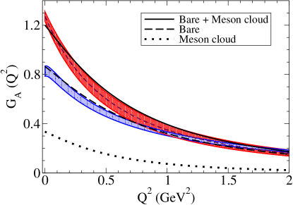
Figure 2: Results of the fit of the axial form factor $G_{A}$ using $g_{A}^{0}=1.2$. The solid-line represent the function $G_{A}$, the dashed-line represent the bare contribution, $c_{3}\,G_{A}^{\rm B}$, and the dotted-line meson cloud contribution, $c_{5}\,G_{M}^{\rm MC}$. The red and blue bands have the same meaning of Fig. 1.

We consider three fits to the functions $G_{A}^{\rm exp}$ and $G_{A}^{\rm B}$. First, we consider a free fit using the parametrizations described below, which fails to describe the low $Q^{2}$ region of $G_{A}$. In a second fit, we attempt to describe in more detail $G_{A}^{\rm exp}$ near $Q^{2}=0$, imposing $G_{A}(0)=1.2723$, but overestimate the $G_{A}^{\rm B}$ parametrization. Finally, we consider an intermediate fit which compromises the description of the functions $G_{A}^{\rm exp}$ and $G_{A}^{\rm B}$.

In a global fit with no constraints in $g_{A}^{0}$ using the empirical parametrization (2), we obtain $g_{A}^{0}=1.125$ [error of 3% for $G_{A}(0)$]. The remaining parameters are presented in the last row of Table 1. Note, in particular, that in this fit the contribution of the meson cloud in the physical nucleon state is 26% ($c_{5}=1-c_{3}\simeq 0.26$), and that the fit to the function $G_{A}^{\rm B}$ has a chi-square per datapoint of 1.65. Since the parametrization gives $G_{A}(0)=g_{A}^{0}=1.125$, we can conclude that this fit underestimates the experimental data near $Q^{2}=0$ (the experimental value is 1.2723).

To improve the description of $G_{A}$ near $Q^{2}=0$, one needs to constrain the values of $g_{A}^{0}$ to values closer to the experimental value for $G_{A}(0)$. This can be done varying the values of $\eta_{A}$ and $c_{3}$, and keeping $g_{A}^{0}=1.2723$. In this case, one obtains $c_{3}=0.702$, (first row in Table 1), but decreases the quality of the description of the component $G_{A}^{\rm B}$ (chi-square per data point of 2.54).

Finally, we consider a parametrization with an intermediate $g_{A}^{0}$, using $g_{A}^{0}=1.2$. In this case we also obtain a description of $G_{A}^{\rm exp}$ closer to the range of one standard deviation and also a fair description of the function $G_{A}^{\rm B}$ (chi-square per datapoint of 2.06). The contribution of the meson cloud in the physical nucleon is in this case 28% (second row in Table 1).

The graphical representation of the last parametrization is presented in Fig. 2. The function $G_{A}$ is represented by the solid-line; the function $c_{3}G_{A}^{\rm B}$ is represented by the dashed-line, and the meson cloud contribution $c_{5}G_{A}^{\rm MC}$ is represented by the dotted-line.

From Fig. 2, one can conclude that the fit associated with $g_{A}^{0}=1.2$ provides the simultaneous description of the parametrizations $G_{A}^{\rm exp}$ and $G_{A}^{\rm B}$ (red and blue bands, respectively), since the lines associated with $G_{A}$ (solid-line) and $G_{A}^{\rm B}$ (dotted-line) are almost always inside the respective bands (one standard deviation). One can also see, that the meson cloud contribution (dotted-line) falls off faster than the bare contribution (dashed-line). This falloff is discussed in more detail in the following sections.

The parametrization from Fig. 2 corresponds to a meson cloud admixture coefficient $c_{3}=Z_{N}=0.72$, meaning that the meson cloud component accounts for 28% of the physical nucleon state, as mentioned above. This estimate is very close to the estimates from the spectator model from Ref. AxialFF (27%) and also from the Cloudy Bag Model from Ref. Shanahan13 (29%). The estimates from the perturbative chiral quark model Liu15a ; Liu16a are also similar to our results for the bare and meson cloud contributions to the nucleon axial form factors, at low $Q^{2}$.

We can then conclude that our estimate of the amount of the meson cloud is close to other estimates of the that effect (around 30%).

IV.3 Discussion about $g_{A}^{0}$

We now discuss in more detail the effect of the parameter $g_{A}^{0}$ in the calculations. As mentioned previously, the holographic results for $G_{A}(Q^{2})$ are strongly dependent on $g_{A}^{0}$. Large values of $g_{A}^{0}$ ($g_{A}^{0}>1.3$) overestimate the low $Q^{2}$ data. Small values of $g_{A}^{0}$ ($g_{A}^{0}<1.1$) underestimate the low $Q^{2}$ data. The constraints from lattice QCD favors values of $g_{A}^{0}$ smaller than 1.27. Recall that the results obtained in lattice QCD simulations for $G_{A}(0)$ are in general restricted to $G_{A}(0)=1.1$–1.2.

In order to check the range of $g_{A}^{0}$ preferred by the lattice data, we start by comparing the holographic models directly with the lattice QCD data. Notice that the holographic model includes a bare and a meson cloud component. Since the $Q^{2}$-dependence of the lattice data varies with the pion mass, we select lattice QCD data associated with the pion masses not to far way from the physical limit. We consider in particular data associated with $m_{\pi}=213$, 260 and 262 MeV from Refs. Alexandrou13 ; Alexandrou11a .

The comparison with the lattice QCD data is presented in Fig. 3 for the parametrizations from Table 1, labeled by $g_{A}^{0}=1.125$, 1.2 and 1.273. In the figure we can observe a good agreement with the data for the parametrizations with $g_{A}^{0}=1.125$ and 1.2 below $Q^{2}=0.3$ GeV², and a systematic deviation for larger values of $Q^{2}$ for all the parametrizations.

There are in principle two main reasons for the deviation between the lattice data and the holographic estimates. On one hand the holographic model under discussion is developed for the physical limit. Therefore the bare and the meson cloud components are estimates for $m_{\pi}=m_{\pi}^{\rm phys}$, and not for higher values of $m_{\pi}$. On the other hand, it is well known that in lattice QCD simulations with large pion masses, the meson cloud effects effects are suppressed. In these conditions, although one may expect that the valence quark component for $m_{\pi}\approx 300$ MeV provide a close estimate for the valence quark component at the physical limit, for the meson cloud component one can expect a stronger dependence on the pion mass due to chiral effects.

To summarize, the deviation between the holographic parametrizations from the lattice QCD data can be interpreted mainly as a consequence of the suppression of the meson cloud effects in the lattice QCD simulations.

To test if the deviation of the holographic model from the lattice data is in fact the result of the dominance of the valence quark contribution in the lattice data, we compare directly the model parametrizations for the valence quark contributions with the results of the lattice QCD simulations.

To help the discussion, we rewrite Eq. (14) as

$$G_{A}(Q^{2})=G_{A}^{\rm B}(Q^{2})+(1-c_{3})\left[G_{A}^{\rm MC}(Q^{2})-G_{A}^{\rm B}(Q^{2})\right].$$

(21)

In the present form, the second term can be seen as the alternative representation of the meson cloud contribution, defined by the difference between $G_{A}$ and $G_{A}^{\rm B}$, when all the normalization factors are taken into account ($Z_{N}=c_{3}$). Notice that the second term in Eq. (21) vanishes at $Q^{2}=0$, as a consequence of the normalization of $G_{A}^{\rm B}$ and $G_{A}^{\rm MC}$ (reduced to $g_{A}^{0}$ when $Q^{2}=0$).

Equation (21) provides also a simple illustration of the limit where the system is completely dominated by the valence quark component. In that case $Z_{N}\equiv c_{3}\to 1$, the second term vanishes, and $G_{A}$ is reduced to $G_{A}^{\rm B}$, as expected.

The direct comparison between the parametrizations of the valence quark contribution with the lattice QCD data is presented in Fig. 4. From the figure, we can conclude that the models with larger $g_{A}^{0}$ overestimates the lattice data near $Q^{2}=0$. Only the models with the values $g_{A}^{0}=1.125$ and 1.2 are closer to the lattice data for $Q^{2}<0.2$ GeV². Between those parametrizations, $g_{A}^{0}=1.2$ is the one that gives the best description of the lattice QCD data, as can be observed in Fig. 4.

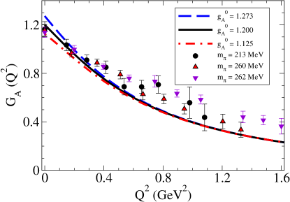
Figure 3: Comparison of the holographic models (full result) with the lattice QCD data Alexandrou13 ; Alexandrou11a . The models are labeled with the value of $g_{A}^{0}$ presented in Table 1.

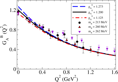
Figure 4: Comparison of $G_{A}^{\rm B}$ with the lattice QCD data Alexandrou13 ; Alexandrou11a . The models are labeled with the value of $g_{A}^{0}$ presented in Table 1.

Overall, the agreement between the estimate of the valence quark contributions and the lattice QCD data is better than the previous case, where we compared the full result (bare plus meson cloud) with the lattice QCD data. Notice, in particular the good agreement between the estimates at large $Q^{2}$ for the datasets with $m_{\pi}=213$ and 260 MeV. These results suggest that the second term in Eq. (21), has a small magnitude in the lattice QCD simulations for pion masses around 0.23 GeV. Notice also that the term under discussion is negative because $G_{A}^{\rm MC}$ has a faster falloff than $G_{A}^{\rm B}$. As a consequence, the values of $G_{A}$ increase, when the term is neglected (compare Figs. 3 and 4).

Looking in particular for the data associated with the largest pion mass ($m_{\pi}=262$ MeV), we can notice that the function $G_{A}^{B}$ (estimated for $m_{\pi}^{\rm phys}$) falls off faster with $Q^{2}$ than the lattice QCD data. The same effect happens for simulations with $m_{\pi}>300$ MeV (not shown here). This effect has been observed in several lattice QCD studies. Lattice QCD calculations of form factors associated with large pion masses have slower falloffs than in the case of the physical form factors NucleonMC3 ; Octet2 ; Lattice ; Yamazaki09 ; Alexandrou13 ; Sasaki08 .

The differences between the lattice QCD data associated with $m_{\pi}=$ 260 and 262 MeV (close values), displayed in Figs. 3 and 4, suggest that the estimation of the valence quark and meson cloud contributions for $G_{A}$ should not be performed based on only a few lattice QCD datasets. It is then preferable to use a significant number of datasets with different values for the pion masses, or in alternative to consider an extrapolation of the lattice QCD results based on several datasets, as discussed in Sec. II.4.

The present analysis does not imply that the lattice QCD simulations with $m_{\pi}\approx 0.2$ GeV have no meson cloud contributions, it shows only that those contributions seem to be small or of the order of the errorbars. Those effects are expected to became more significant when we approach the physical limit.

The comparison between the bare contribution of the holographic model with the lattice QCD data, and their close agreement, justifies the choice of values of $g_{A}^{0}$ smaller than the experimental value, namely $g_{A}^{0}\simeq 1.2$. This result confirms also the need to use constraints in the function $G_{A}^{\rm B}$, in order to obtain a better description of the physics associated with the axial form factor $G_{A}$.

A choice of values of $g_{A}^{0}$ below 1.27 may also be justified by dynamical effects in the quark structure. Calculations based on the Dyson-Schwinger framework show a reduction of the quark axial charge $g_{A}^{q}$ due to the gluon dressing of the quarks. As a consequence the valence quark contribution to $G_{A}$ is reduced when compared to calculations based on undressed quarks Eichmann12 ; Chang13 ; Yamanaka14 .

IV.4 Vector meson dominance models

In the literature we can find some models for the axial form factor based on VMD with axial-vector mass poles Hong07 ; Hashimoto08 ; Adamuscin08 . The models from Refs. Hong07 ; Adamuscin08 are called two-component models, and include a term associated with the lowest axial-vector meson state ($a_{1}$). Those models explore also the possible decompositions between a bare core component and a component associated with the (axial-vector) meson cloud. The model estimates are compatible with the parametrization (2) below 1 GeV². The holographic model from Ref. Hashimoto08 considers an expansion in the axial-vector meson poles. In that case it was shown that the final expression for $G_{A}$ can also be approximated by a dipole, at low $Q^{2}$.

IV.5 Estimate of the meson cloud contribution from holography

Finally, we discuss the estimate of the meson cloud contribution associated with the our best holographic model ($g_{A}^{0}=1.2$). The meson cloud contribution to the axial form factor was already shown in Fig. 2. In that figure we can see, looking at the meson cloud contribution (dotted-line) that $G_{A}^{\rm MC}$ does not fall to zero very fast. One can also conclude that for large $Q^{2}$, the holographic estimate of the bare contribution underestimates the result of the spectator model from Ref. AxialFF , defined by the central value of the blue band.

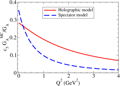
Figure 5: Comparison between the relative contributions of the meson cloud in the holographic model and in the spectator model.

The previous result suggests that the holographic estimate of the meson cloud has a slow falloff compared to the estimate from the spectator model, determined by Eq. (6) AxialFF . This effect can be observed in more detail in Fig. 5, where we plot the ratio between $c_{5}G_{A}^{\rm MC}$ and $G_{A}$, estimated by the respective model, up to $Q^{2}=4$ GeV². In this representation the difference between falloffs became clear. Apart the difference between parametrizations at $Q^{2}=0$, which are compatible with the uncertainties of the estimates of $G_{A}^{\rm exp}$ and $G_{A}^{\rm B}$, it is clear in the graph the difference of falloffs between the spectator model (fast) and our best holographic model (slow).

We recall that both estimates of the meson cloud fall off with $1/Q^{8}$ for large $Q^{2}$ (faster than the valence quark contributions: $1/Q^{4}$). The multiplicative factors associated with those functions in the holographic and spectator models are, however, very different. The factor associated with the holographic model is larger than the one from the spectator model.

A quantitative measure of the falloff from the meson cloud contribution may be the value of $Q^{2}$ for which the contribution of the meson cloud becomes smaller than 10% of $G_{A}(Q^{2})$. From Fig. 5, we can conclude that this value is about 1 GeV² for the spectator model, and about 2.8 GeV² for the holographic model.

The meson cloud estimate from the perturbative chiral quark model has a falloff even slower than the holographic model. For $Q^{2}\simeq 1$ GeV² the meson cloud contribution dominates over the bare contribution Liu15a ; Liu16a . According to Ref. Liu16a the flat behavior of the meson cloud contribution (slow falloff) may indicate that the meson cloud distribution is closer to the origin in the coordinate space, than in other models. The calculation based on the holographic model, and the faster falloff of the meson cloud contribution, suggests a much more peripheral distribution of the meson cloud.

The difference between the falloffs in holographic models and quark models may be a consequence of the way the meson structure is described. In the holographic models the substructure associated with the $q\bar{q}$ pair is neglected in first approximation, meaning that the meson states are regarded as pointlike particles. In the quark models, the mesons are extended particles with structure form factors that can be approximated by multipole functions. Those multipole functions are parametrized by cutoffs that characterize the spatial extension of the mesons and are also responsible for the faster falloff of the meson cloud contribution, compared to models with pointlike mesons.

V Outlook and conclusions

In the present work we study the structure of the nucleon axial form factor using the formalism of the light-front holography. In a holographic model the substructure associated with the valence quark degrees of freedom and the substructure associated with the meson cloud excitations are both parametrized in terms of two independent microscopic couplings: $g_{A}^{0}$, the quark axial-vector coupling, and $\eta_{A}$ the quark induced pseudoscalar coupling. Contrary to the case of the quark models with meson cloud dressing, in the holographic models there is no explicit connection with the baryon-meson substructure.

We checked if the empirical information associated with the nucleon axial form factor $G_{A}$ could be used to determine the fraction of $G_{A}$ associated with the valence quark components ($G_{A}^{\rm B}$) and the fraction associated with the meson cloud component ($G_{A}^{\rm MC}$), based on a holographic model. We concluded that this goal can be achieved if we use the information from lattice QCD simulations to constraint the bare component, associated with the valence quark degrees of freedom.

We realized also that the results from the bare and the meson cloud components of $G_{A}$ depend crucially on the coupling $g_{A}^{0}$. Large values of $g_{A}^{0}$ fail to describe the magnitude of the function $G_{A}^{\rm B}$, extracted from lattice QCD. Small values of $g_{A}^{0}$ fail to describe the empirical data.

A good compromise in the description of the experimental data and the estimate of $G_{A}^{\rm B}$ is obtained when we use $g_{A}^{0}\simeq 1.2$, $\eta_{A}\simeq 1.1$ and a meson cloud mixture of about 30% in the physical nucleon state. A holographic model with $g_{A}^{0}\simeq 1.2$, provides also a parametrization more consistent with the results from lattice QCD. Most of lattice QCD simulations give $G_{A}(0)=1.1$–1.2, in a wide range of pion masses ($m_{\pi}=0.2$–0.5 GeV).

To summarize, the holographic model presented here provides a consistent description of the $G_{A}$ data and from the estimate of the bare contribution extracted from lattice QCD. In addition, the holographic model provides a parametrization for the meson cloud contributions to $G_{A}$.

The holographic estimate of $G_{A}^{\rm MC}$ has a very slow falloff with $Q^{2}$. The meson cloud contribution is smaller than 10% of $G_{A}$ only for large values of $Q^{2}$ ($Q^{2}>2.8$ GeV²). In other quark models with meson cloud dressing this reduction happens typically for values of $Q^{2}$ larger than 1 GeV².

In the future, it will be very interesting to check if also for the electromagnetic form factors estimated by holographic models, the falloff of the meson cloud contribution is very slow as for the nucleon axial form $G_{A}$, or if the falloff is faster, as suggested by some quark models.

- (1) J. M. Maldacena, Int. J. Theor. Phys. 38, 1113 (1999) [Adv. Theor. Math. Phys. 2, 231 (1998)] [hep-th/9711200].
- (2) E. Witten, Adv. Theor. Math. Phys. 2, 253 (1998) [hep-th/9802150].
- (3) S. S. Gubser, I. R. Klebanov and A. M. Polyakov, Phys. Lett. B 428, 105 (1998) [hep-th/9802109].
- (4) S. J. Brodsky, G. F. de Teramond, H. G. Dosch and J. Erlich, Phys. Rept. 584, 1 (2015) [arXiv:1407.8131 [hep-ph]].
- (5) S. J. Brodsky and G. F. de Teramond, Phys. Rev. D 77, 056007 (2008) [arXiv:0707.3859 [hep-ph]].
- (6) G. F. de Teramond and S. J. Brodsky, Phys. Rev. Lett. 102, 081601 (2009) [arXiv:0809.4899 [hep-ph]].
- (7) A. Karch, E. Katz, D. T. Son and M. A. Stephanov, Phys. Rev. D 74, 015005 (2006) [hep-ph/0602229].
- (8) H. R. Grigoryan and A. V. Radyushkin, Phys. Rev. D 76, 095007 (2007) [arXiv:0706.1543 [hep-ph]].
- (9) T. Branz, T. Gutsche, V. E. Lyubovitskij, I. Schmidt and A. Vega, Phys. Rev. D 82, 074022 (2010) [arXiv:1008.0268 [hep-ph]].
- (10) T. Gutsche, V. E. Lyubovitskij, I. Schmidt and A. Vega, Phys. Rev. D 85, 076003 (2012) [arXiv:1108.0346 [hep-ph]].
- (11) G. F. de Teramond, H. G. Dosch and S. J. Brodsky, Phys. Rev. D 91, 045040 (2015) [arXiv:1411.5243 [hep-ph]].
- (12) D. Chakrabarti and C. Mondal, Eur. Phys. J. C 73, 2671 (2013) [arXiv:1307.7995 [hep-ph]].
- (13) Z. Abidin and C. E. Carlson, Phys. Rev. D 79, 115003 (2009) [arXiv:0903.4818 [hep-ph]].
- (14) G. F. de Teramond and S. J. Brodsky, AIP Conf. Proc. 1432, 168 (2012) [arXiv:1108.0965 [hep-ph]].
- (15) T. Liu and B. Q. Ma, Phys. Rev. D 92, 096003 (2015) [arXiv:1510.07783 [hep-ph]].
- (16) T. Gutsche, V. E. Lyubovitskij, I. Schmidt and A. Vega, Phys. Rev. D 86, 036007 (2012) [arXiv:1204.6612 [hep-ph]].
- (17) T. Gutsche, V. E. Lyubovitskij, I. Schmidt and A. Vega, Phys. Rev. D 87, 016017 (2013) [arXiv:1212.6252 [hep-ph]].
- (18) R. S. Sufian, G. F. de Teramond, S. J. Brodsky, A. Deur and H. G. Dosch, Phys. Rev. D 95, 014011 (2017) [arXiv:1609.06688 [hep-ph]].
- (19) G. Ramalho and D. Melnikov, Phys. Rev. D 97, 034037 (2018) [arXiv:1703.03819 [hep-ph]].
- (20) G. Ramalho, Phys. Rev. D 96, 054021 (2017) [arXiv:1706.05707 [hep-ph]].
- (21) A. Vega, I. Schmidt, T. Gutsche and V. E. Lyubovitskij, Phys. Rev. D 83, 036001 (2011) [arXiv:1010.2815 [hep-ph]].
- (22) D. Chakrabarti and C. Mondal, Phys. Rev. D 88, 073006 (2013) [arXiv:1307.5128 [hep-ph]].
- (23) G. A. Miller, Phys. Rev. C 66, 032201 (2002) [nucl-th/0207007]
- (24) F. Gross, G. Ramalho and K. Tsushima, Phys. Lett. B 690, 183 (2010) [arXiv:0910.2171 [hep-ph]].
- (25) G. Ramalho and K. Tsushima, Phys. Rev. D 84, 054014 (2011) [arXiv:1107.1791 [hep-ph]].
- (26) G. Ramalho and K. Tsushima, Phys. Rev. D 94, 014001 (2016) [arXiv:1512.01167 [hep-ph]].
- (27) V. Bernard, L. Elouadrhiri and U. G. Meissner, J. Phys. G 28, R1 (2002) [hep-ph/0107088].
- (28) M. R. Schindler and S. Scherer, Eur. Phys. J. A 32, 429 (2007) [hep-ph/0608325].
- (29) T. Gorringe and H. W. Fearing, Rev. Mod. Phys. 76, 31 (2003) [nucl-th/0206039].
- (30) K. A. Olive et al. [Particle Data Group Collaboration], Chin. Phys. C 38, 090001 (2014).
- (31) I. G. Aznauryan et al., Int. J. Mod. Phys. E 22, 1330015 (2013) [arXiv:1212.4891 [nucl-th]].
- (32) J. M. Gaillard and G. Sauvage, Ann. Rev. Nucl. Part. Sci. 34, 351 (1984).
- (33) B. Julia-Diaz, D. O. Riska and F. Coester, Phys. Rev. C 70, 045204 (2004) [nucl-th/0406015].
- (34) C. Adamuscin, E. Tomasi-Gustafsson, E. Santopinto and R. Bijker, Phys. Rev. C 78, 035201 (2008) [arXiv:0706.3509 [nucl-th]].
- (35) A. W. Thomas, Adv. Nucl. Phys. 13, 1 (1984); S. Theberge and A. W. Thomas, Nucl. Phys. A 393, 252 (1983).
- (36) K. Tsushima, T. Yamaguchi, Y. Kohyama and K. Kubodera, Nucl. Phys. A 489, 557 (1988).
- (37) P. E. Shanahan, A. W. Thomas, K. Tsushima, R. D. Young and F. Myhrer, Phys. Rev. Lett. 110, 202001 (2013) [arXiv:1302.6300 [nucl-th]].
- (38) F. Schlumpf, Phys. Rev. D 47, 4114 (1993) [Phys. Rev. D 49, 6246 (1994)] [hep-ph/9212250].
- (39) S. Boffi, L. Y. Glozman, W. Klink, W. Plessas, M. Radici and R. F. Wagenbrunn, Eur. Phys. J. A 14, 17 (2002) [hep-ph/0108271].
- (40) D. Merten, U. Loring, K. Kretzschmar, B. Metsch and H. R. Petry, Eur. Phys. J. A 14, 477 (2002) [hep-ph/0204024].
- (41) D. Barquilla-Cano, A. J. Buchmann and E. Hernandez, Nucl. Phys. A 714, 611 (2003) [nucl-th/0204067].
- (42) A. Silva, H. C. Kim, D. Urbano and K. Goeke, Phys. Rev. D 72, 094011 (2005) [hep-ph/0509281].
- (43) B. Pasquini and S. Boffi, Phys. Rev. D 76, 074011 (2007) [arXiv:0707.2897 [hep-ph]].
- (44) H. Dahiya and M. Randhawa, Phys. Rev. D 90, 074001 (2014) [arXiv:1409.4943 [hep-ph]].
- (45) I. V. Anikin, V. M. Braun and N. Offen, Phys. Rev. D 94, 034011 (2016) [arXiv:1607.01504 [hep-ph]].
- (46) X. Y. Liu, K. Khosonthongkee, A. Limphirat, P. Suebka and Y. Yan, Phys. Rev. D 91, 034022 (2015) [arXiv:1406.7633 [hep-ph]].
- (47) X. Y. Liu, K. Khosonthongkee, A. Limphirat and Y. Yan, arXiv:1601.01428 [hep-ph].
- (48) G. Eichmann and C. S. Fischer, Eur. Phys. J. A 48, 9 (2012) [arXiv:1111.2614 [hep-ph]].
- (49) L. Chang, C. D. Roberts and S. M. Schmidt, Phys. Rev. C 87, 015203 (2013) [arXiv:1207.5300 [nucl-th]].
- (50) N. Yamanaka, S. Imai, T. M. Doi and H. Suganuma, Phys. Rev. D 89, 074017 (2014) [arXiv:1401.2852 [hep-ph]].
- (51) S. Mamedov, B. B. Sirvanli, I. Atayev and N. Huseynova, Int. J. Theor. Phys. (2017) arXiv:1609.00167 [hep-th].
- (52) S. Sasaki et al. [RIKEN-BNL-Columbia-KEK Collaboration], Phys. Rev. D 68, 054509 (2003) [hep-lat/0306007].
- (53) R. G. Edwards et al. [LHPC Collaboration], Phys. Rev. Lett. 96, 052001 (2006) [hep-lat/0510062].
- (54) T. Yamazaki et al. [RBC+UKQCD Collaboration], Phys. Rev. Lett. 100, 171602 (2008) [arXiv:0801.4016 [hep-lat]].
- (55) T. Bhattacharya, S. D. Cohen, R. Gupta, A. Joseph, H. W. Lin and B. Yoon, Phys. Rev. D 89, 094502 (2014) [arXiv:1306.5435 [hep-lat]].
- (56) J. Liang, Y. B. Yang, K. F. Liu, A. Alexandru, T. Draper and R. S. Sufian, arXiv:1612.04388 [hep-lat].
- (57) S. Sasaki and T. Yamazaki, Phys. Rev. D 78, 014510 (2008) [arXiv:0709.3150 [hep-lat]].
- (58) T. Yamazaki, Y. Aoki, T. Blum, H. W. Lin, S. Ohta, S. Sasaki, R. Tweedie and J. Zanotti, Phys. Rev. D 79, 114505 (2009) [arXiv:0904.2039 [hep-lat]].
- (59) J. D. Bratt et al. [LHPC Collaboration], Phys. Rev. D 82, 094502 (2010) [arXiv:1001.3620 [hep-lat]].
- (60) C. Alexandrou, M. Constantinou, S. Dinter, V. Drach, K. Jansen, C. Kallidonis and G. Koutsou, Phys. Rev. D 88, 014509 (2013) [arXiv:1303.5979 [hep-lat]].
- (61) C. Alexandrou et al. [ETM Collaboration], Phys. Rev. D 83, 045010 (2011) [arXiv:1012.0857 [hep-lat]].
- (62) J. Green et al., Phys. Rev. D 95, 114502 (2017) [arXiv:1703.06703 [hep-lat]].
- (63) R. Horsley, Y. Nakamura, A. Nobile, P. E. L. Rakow, G. Schierholz and J. M. Zanotti, Phys. Lett. B 732, 41 (2014) [arXiv:1302.2233 [hep-lat]].
- (64) A. Abdel-Rehim et al., Phys. Rev. D 92, 114513, (2015) Erratum: [Phys. Rev. D 93, 039904 (2016)] [arXiv:1507.04936 [hep-lat]].
- (65) G. S. Bali et al., Phys. Rev. D 91, 054501 (2015) [arXiv:1412.7336 [hep-lat]].
- (66) T. Bhattacharya, V. Cirigliano, S. Cohen, R. Gupta, H. W. Lin and B. Yoon, Phys. Rev. D 94, 054508 (2016) [arXiv:1606.07049 [hep-lat]].
- (67) S. Capitani et al., arXiv:1705.06186 [hep-lat].
- (68) E. Berkowitz et al., arXiv:1704.01114 [hep-lat].
- (69) D. L. Yao, L. Alvarez-Ruso and M. J. Vicente-Vacas, arXiv:1708.08776 [hep-ph].
- (70) K. Park et al. [CLAS Collaboration], Phys. Rev. C 85, 035208 (2012) [arXiv:1201.0903 [nucl-ex]].
- (71) F. Gross, G. Ramalho and M. T. Peña, Phys. Rev. C 77, 015202 (2008) [nucl-th/0606029].
- (72) G. Ramalho, K. Tsushima and F. Gross, Phys. Rev. D 80, 033004 (2009) [arXiv:0907.1060 [hep-ph]].
- (73) G. Ramalho and M. T. Peña, Phys. Rev. D 83, 054011 (2011) [arXiv:1012.2168 [hep-ph]].
- (74) G. Ramalho and M. T. Peña, J. Phys. G 36, 115011 (2009) [arXiv:0812.0187 [hep-ph]].
- (75) G. Ramalho and M. T. Peña, Phys. Rev. D 80, 013008 (2009) [arXiv:0901.4310 [hep-ph]].
- (76) G. Ramalho, K. Tsushima and A. W. Thomas, J. Phys. G 40, 015102 (2013) [arXiv:1206.2207 [hep-ph]].
- (77) T. Sakai and S. Sugimoto, Prog. Theor. Phys. 113, 843 (2005) [hep-th/0412141].
- (78) K. Nawa, H. Suganuma and T. Kojo, Phys. Rev. D 75, 086003 (2007) [hep-th/0612187].
- (79) D. K. Hong, M. Rho, H. U. Yee and P. Yi, JHEP 0709, 063 (2007) [arXiv:0705.2632 [hep-th]].
- (80) K. Hashimoto, T. Sakai and S. Sugimoto, Prog. Theor. Phys. 120, 1093 (2008) [arXiv:0806.3122 [hep-th]].
- (81) D. K. Hong, M. Rho, H. U. Yee and P. Yi, Phys. Rev. D 77, 014030 (2008) [arXiv:0710.4615 [hep-ph]].
- (82) J. J. Sakurai, Annals Phys. 11, 1 (1960).
- (83) T. H. Bauer, R. D. Spital, D. R. Yennie and F. M. Pipkin, Rev. Mod. Phys. 50, 261 (1978) Erratum: [Rev. Mod. Phys. 51, 407 (1979)].
- (84) M. Gari and W. Krumpelmann, Phys. Lett. 141B, 295 (1984).
- (85) E. L. Lomon, Phys. Rev. C 64, 035204 (2001) [nucl-th/0104039].