Sensitivity of the entanglement spectrum to boundary conditions as a characterization of the phase transition from delocalization to localization

Abstract

Sensitivity of entanglement Hamiltonian spectrum to boundary conditions is considered as a phase detection parameter for delocalized-localized phase transition. By employing one-dimensional models that undergo delocalized-localized phase transition, we study the shift in the entanglement energies and the shift in the entanglement entropy when we change boundary conditions from periodic to anti-periodic. Specifically, we show that both these quantities show a change of several orders of magnitude at the transition point in the models considered. Therefore, this shift can be used to indicate the phase transition points in the models. We also show that both these quantities can be used to determine mobility edges separating localized and delocalized states.

I Introduction

Entanglement as a purely quantum phenomenon has been intensively studied for the past decades.ref:Horodecki It is thought to underlie modern technologies such as quantum computing and cryptography, to name a few.ref:chuang ; ref:Ekert ; ref:Steane ; ref:Gisin Recently, entanglement has been used intensively to study condensed-matter systems as well. Entanglement is a measure of how much quantum correlation exists in multipartite quantum system. In condensed-matter, systems that exhibit continuous phase transition are marked by a critical point, where the system becomes highly correlated with power-law (long-range) correlations. It is therefore not surprising that entanglement can be used as a parameter to characterize phase transition and critical points in quantum many-body system,ref:osterloh ; ref:amico ; ref:haque ; ref:kitaev although there exist some debates.ref:chandran ; ref:min-fongyang

There are several measures of entanglementref:vedral by which various authors have characterized different phases and phase transitions.ref:vidal ; ref:osborne ; ref:shi ; ref:vidal2 von Neumann entanglement entropy (EE), as the most popular and standard measure of entanglement in a pure state, has been frequently used. In a bipartite approach, one can partition the system in various ways, as in momentum space, ref:mondragon ; ref:andrade or a combination of momentum and orbital partition, ref:mondragon2 or various other choices. ref:othercut In addition, other authors have advocated a multipartite approach where entanglement finds a more (extensive) thermodynamic interpretation. ref:wei ; ref:love ; ref:chhajlany ; ref:afshin1 ; ref:afshin2 People also use spectrum of the reduced density matrix ref:LiHaldane to distinguish different phases. In addition, it is also shown that eigen-modes of the entanglement Hamiltonian may carry some useful physics.ref:pouranvariyang1 ; ref:pouranvariyang2 ; ref:pouranvariyang5

Among the various phase transitions in condensed-matter physics, Anderson phase transition between a localized and an extended (delocalized) phase is of particular interest. Various authors have also studied such a transition in the light of entanglement. For example, in Ref. [ref:berkovitsprl2015, ] the probability distribution of the EE is used to characterize different phases in a one-dimensional wire with attractive interaction. In Ref. [ref:chakravarty, ] it is shown that EE is non-analytic at the delocalized-localized phase transition point. A finite-size scaling of the EE is done in Ref. [ref:zhao, ] to characterize the Anderson transition and to obtain the critical exponents. The dependence of the EE upon mean free path in a free fermion model and upon the localization length in interacting model with Anderson transition is studied in Ref. [ref:pouranvariyang4, ] and Ref. [ref:berkovitsprl2012, ], respectively. More recently, the role of the entanglement in interacting models and its relation to thermalization has been emphasized. ref:bardarson ; ref:nag ; ref:filho ; ref:geraedts ; ref:khemani ; ref:yang ; ref:berkovits ; ref:vidmar

In this paper, we intend to study localization-delocalization phase transition by introducing another related quantity as a phase detection parameter, namely the sensitivity of the entanglement energies to boundary condition. Effect of the (sub)system boundary condition on the entanglement properties has been studied before. Here we mention some of these studies: in Ref. [ref:laflorencie2006, ] the effect of the open boundary condition (in contrast to periodic boundary condition) on the entanglement entropy is calculated. Effect of an impurity located on the subsystem boundary is studied for a Luttinger liquid in Ref. [ref:levine, ]. In Ref. [ref:peschel2005, ] defects at the boundary of the subsystem for a tight binding model is considered as impurities on the hopping elements and on-site energies, and their effects on the entanglement spectrum and central charge. Our approach is different from above in a sense that we consider the effect of boundary conditions in different phases, and use this as a detection mechanism for the phase transition.

Regarding delocalized-localized transition, there are several methods to distinguish different phases. The most widely used method is the statistics of the level spacing,ref:Shklovskii which we only need the eigen-energies rather than the eigen-states. In Ref. [ref:edward, ], Edwards and Thouless study the sensitivity of the eigen-energies of a system’s Hamiltonian to the boundary conditions. When boundary conditions change from periodic boundary condition (PBC) to anti-periodic boundary condition (APBC) the shift in the eigen-energies is used to distinguish localized and de-localized phases. The basic idea is the following: if the eigen-mode is localized, it does not “see” the boundaries and thus it is not affected by any change in the boundary conditions and the corresponding eigen-energy does not alter. On the other hand, when the eigen-mode is extended, it is affected by what happens at the boundary; the change in the corresponding eigen-energy being comparable to the spacing between eigen-energies. They used the amount of this shift as a criterion for detecting the Anderson phase transition. This shift in the eigen-energies is related to the transmission and subsequently to the conductance of the system.ref:anderson ; ref:economou ; ref:kramer

On the other hand, there are similarities between the eigen-modes of the Hamiltonian and the eigen-modes of the entanglement Hamiltonian, specially between the eigen-modes of the Hamiltonian at the Fermi level $|E_{F}\rangle$, and the maximally entangled mode $|MEM\rangle$.ref:footenote In Ref. [ref:pouranvariyang2, ] we demonstrated this similarity by employing two one-dimensional free fermion models that exhibit localized-delocalized (LD) phase transition. We found that both $|E_{F}\rangle$ and $|MEM\rangle$ are extended in the delocalized phase and both are localized in the localized phase. Also, their overlap is substantial in the delocalized phase or at least at the phase transition point. In short, eigen-modes of the entanglement Hamiltonian and specially the $|MEM\rangle$ carry on some physics of the $|E_{F}\rangle$. In this paper, we further address this similarity by showing that one can extract localization properties of the system by studying entanglement Hamiltonian instead of Hamiltonian of the system. We conjecture that if the entanglement Hamiltonian eigen-mode is extended the corresponding entanglement energy is affected by the boundary conditions and if it is localized, then the corresponding entanglement energy does not change.

Accordingly, in specific one-dimensional free fermion models that undergo LD phase transition, we change the boundary condition from PBC to APBC and see how the entanglement energies and thus entanglement entropy changes. We show numerically that the shift in the entanglement Hamiltonian spectrum is considerable in the delocalized phase but it is negligible in the localized phase. Thus, it can be used as a characterization of LD phase transition. Furthermore, we also show that the same ideas can be used to identify mobility edges. We would like to mention that the one-dimensional models we consider here have theoretical relevance, but have also recently been found to have experimental relevance as well. ref:diener ; ref:lahini

The remainder of the paper is as follows: in Sec. II, we explain the method for calculating the entanglement spectrum and entanglement entropy. We also explain the one-dimensional models that are used in this paper to verify our conjecture. In Sec. III, we present the main result of this paper: we study the effect of the change in the boundary conditions on entanglement Hamiltonian spectrum, and entanglement entropy. We also show that the shift, only in the smallest magnitude entanglement energy, is enough to characterize the phase transition. As an extra check, for a one-dimensional model with mobility edges, we show that the shift locates the mobility edges for the whole spectrum. We close in Sec. LABEL:conclusion with a summary and concluding remarks.

II Methods and Models

If a system is in a pure state $|\Psi\rangle$, density matrix will be $\rho=|\Psi\rangle\langle\Psi|$. We divide the system into two subsystems $A$ and $B$ and for each subsystem the reduced density matrix is obtained by tracing over degrees of freedom of the other subsystem: $\rho^{A/B}=tr_{B/A}(\rho)$. Block von Neumann entanglement entropy between the two subsystems is $EE=-tr(\rho^{A}\ln{\rho^{A}})=-tr(\rho^{B}\ln{\rho^{B}})$. For a single Slater-determinant ground state, the reduced density matrix of each subsystem can be written as:

$$\rho^{A/B}=\frac{1}{Z}e^{-H^{A/B}},$$ (1)

where $H^{A/B}$ is the free-fermion entanglement Hamiltonians ($Z$ is determined by $tr\rho^{A/B}=1$):

$$H^{A/B}=\sum_{ij}h_{ij}^{A/B}c_{i}^{\dagger}c_{j},$$ (2)

where $c_{i}^{\dagger}(c_{i})$ is the fermionic creation (annihilation) operator for site $i$.

To calculate entanglement energies $\epsilon$’s, i.e. the eigen-values of the $h^{A/B}$ matrix, we use method of Ref. [correl, ]: we divide the system in two parts, subsystem $A$ from site $1$ to $N_{A}$ and the rest as subsystem $B$. We diagonalize the correlation matrix of a subsystem, say $A$

$$C_{i,j}=\left<c_{i}^{\dagger}c_{j}\right>,$$ (3)

(where $i$ and $j$ go from $1$ to $N_{A}$) and find its eigen-values $\{\zeta\}$. Eigen-values of the correlation matrix and those of the entanglement Hamiltonian are related as:

$$\zeta_{i}=\frac{1}{1+e^{\epsilon_{i}}},$$ (4)

and EE will be given as:

$$\text{EE}=-\sum_{i=1}^{N_{A}}[\zeta_{i}\ln(\zeta_{i})+(1-\zeta_{i})\ln(1-\zeta_{i})],$$ (5)

Next, we introduce lattice models we work with in this paper. They are one-dimensional free fermion tight binding models with constant nearest neighbor coupling $t$ and on-site energies $\phi_{n}$:

$$H=t\sum_{n=1}^{N}(c_{n}^{\dagger}c_{n+1}+c_{n+1}^{\dagger}c_{n})+\sum_{n=1}^{N}\phi_{n}c_{n}^{\dagger}c_{n},$$ (6)

The first model is random dimer model (RD)dunalp where $\phi_{n}$’s are randomly chosen from one of two independent on site energies $\phi_{a}$ or $\phi_{b}$. One of the site energies (we choose it to be $\phi_{b}$) is assigned to neighboring pairs of lattice sites. As shown by Dunalp et al.dunalp , when $-2t\leq\phi_{a}-\phi_{b}\leq 2t$, states at the resonant energy, $E_{res}=\phi_{b}$, are delocalized. Here we set $t=-1$ and $\phi_{a}=0$, thus when $-2\leq\phi_{b}\leq 2$ system is delocalized at the resonant energy $E_{F}=E_{res}=\phi_{b}$, and is localized otherwise.

Another model with the Hamiltonian of the form Eq. (6) has on-site energies:

$$\phi_{n}=2\lambda\frac{\cos{(2\pi nb)}}{1-\alpha\cos{(2\pi nb)}},$$ (7)

where $b=\frac{1+\sqrt{5}}{2}$ is the golden ratio, so that it has incommensurate period with respect to lattice period (we set the lattice constant to be $1$). This model is neither completely periodic (with extended eigen-modes) nor completely random (with localized eigen-modes) and, as illustrated in Ref. [ref:dassarma, ], it has mobility edges separating localized and delocalized states at:

$$E_{\text{mobility edge}}=\frac{2sgn(\lambda)(|t|-|\lambda|)}{\alpha},$$ (8)

where in our calculation we set $t=-1$.

An special case of Eq. (7) with $\alpha=0$ is the Aubry-Andre (AA) modelref:aubryandre which has a phase transition at $\lambda=1$. All eigen-states for $\lambda<1$ are delocalized whereas they become all localized for $\lambda>1$. Thus the AA model does not have mobility edges.

III Sensitivity of Entanglement Properties to Boundary Condition

As mentioned above, Edward and Thoulessref:edward used the sensitivity of the eigen-energies of the system’s Hamiltonian to boundary conditions to distinguish localized from delocalized phases. They used the geometrical average of shifts in the whole spectrum. For comparison with our method, we calculate the magnitude of shift of the eigen-energy at the Fermi level $|\delta E|$ when we change the boundary conditions. In our one-dimensional models we apply PBC by imposing $\psi_{N+1}=+\psi_{1}$ and APBC by $\psi_{N+1}=-\psi_{1}$. The results are plotted in Fig. 1. For both RD and AA models $|\delta E|$ in the delocalized phase is non-zero, it gradually becomes smaller as we approach the phase transition point, and in the localized phase it becomes zero. As seen in Fig. 1, $|\delta E|$ behaves much as an order parameter in standard phase transition.

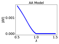
Figure 1: Left panel: disorder average of magnitude of shift in the Hamiltonian eigen-energy at the Fermi level for RD model when we change boundary condition from PBC to APBC as a function of $\phi_{b}$. System size $N=1000$, disorder average is over $1000$ samples. Right panel: magnitude of shift in the Hamiltonian eigen-energy at the Fermi level for AA model as a function of $\lambda$. System size $N=2000$.

III.1 Shift in the Entanglement Hamiltonian Spectrum and Entanglement Entropy

To study the sensitivity of the entanglement to the boundary conditions, let us first examine the spectrum of the entanglement Hamiltonian $\{\epsilon\}$ of one subsystem (here we choose subsystem $A$) when we change boundary condition from PBC to APBC. In Fig. 2, we plot spectrum of the entanglement Hamiltonian in RD model for both cases of PBC and APBC at two different $\phi_{b}$’s. We choose a $\phi_{b}=0.5$ in the delocalized phase and a $\phi_{b}=3.5$ in the localized phase. Only one sample is considered at each $\phi_{b}$. There is a shift between two spectra in the delocalized phase, whereas they are the same in the localized phase — not for the whole spectrum but at least for those $\epsilon$’s close to zero, which are more important since they have more contributions to the entanglement entropy EE, Eq. (5).

Figure 2: (color online) eigen-values of entanglement Hamiltonian of RD model for $\phi_{b}=0.5$ (in delocalized phase) and for $\phi_{b}=3.5$ (in localized phase). Spectrum with PBC is plotted in blue, and with APBC in red. Inset plots are zoomed plots to show a few eigen-values close to zero. At each $\phi_{b}$ only one sample is considered without taking disorder average. We choose $N=60,N_{A}=30$.

r16ptt16pt   r16ptt16pt

To see the shift in the spectrum more quantitatively, we calculate the magnitude of shift in the entanglement entropy $|\delta EE|$ for both RD and AA models, when we change boundary condition (see Fig. 3). Since in the delocalized phase, the spectrum is modified, the change in the entanglement entropy is non-zero, although very small compare to the EE value at each point. But, in the localized phase the change is much smaller and very close to zero.

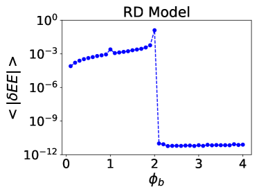
Figure 3: Left panel: disorder average of magnitude of shift in the entanglement entropy $<|\delta EE|>$ when we change boundary condition from PBC to APBC for RD model. In the delocalized phase EE $\sim$ 2.5 and in the localized phase EE $\sim$ 0.5. $N=1000$. Right panel: magnitude of shift in EE $|\delta EE|$ for AA model. In the delocalized phase EE $\sim$ 2.2 and in the localized phase EE $\sim$ 0.4. $N=2000$.

III.2 Shift in the Smallest Magnitude Entanglement Energy

Now, we focus on the smallest magnitude entanglement energy, the $\epsilon$ which is closest to zero and has the most contribution to the EE, Eq. (5). We change the boundary condition from PBC to APBC and measure the magnitude of shift in the lowest magnitude entanglement energy $|\delta\epsilon|$ (and the corresponding $|\delta\zeta|$). For the RD model we plot this shift as a function of $\phi_{b}$ in Fig. 4. Whereas this shift in the delocalized phase (i.e. when $\phi_{b}<2$) is large, it is zero in the localized phase (it is on the order of $10^{-13}$ for the chosen system size). Also for the AA model $|\delta\epsilon|$ (and corresponding $|\delta\zeta|$) is plotted in Fig. 4. The same behavior of $|\delta\epsilon|$ is seen in this model as well.

For both models, we see the shift in the smallest magnitude of the entanglement energy, sharply determines the phase transition point. In the delocalized phase $|\delta\epsilon|$ is non-zero and at the transition pint to localized phase it sharply goes to zero. Calculation of the $|\delta\epsilon|$ to determine the phase transition point is numerically more economical rather than calculation of the $|\delta EE|$ – where we have to obtain the entire spectrum – specially that there are numerical packages (like ARPACK) by which we can obtain the smallest eigen-value efficiently.

Figure 4: Left panel: disorder average of magnitude of shift in the smallest magnitude entanglement energy $<|\delta\epsilon|>$ when we change PBC to APBC for RD model as function of $\phi_{b}$. States are delocalized when $\phi_{b}<2$ and are localized when $\phi_{b}>2$. System size $N=1000$. Disorder average is over $1000$ samples. Standard deviation of $|\delta\epsilon|$ is plotted in lower inset plot. Upper inset plot is the corresponding change in $\zeta$. Right panel: magnitude of Shift in the smallest magnitude entanglement energy $|\delta\epsilon|$ when we change PBC to APBC for AA model as function of $\lambda$. States are delocalized when $\lambda<1$ and are localized when $\lambda>1$. Inset plot is the corresponding change in $\zeta$. $N=2000$.

r7ptt15pt   r7ptt15pt

Next, we consider a model that has mobility edges (contrary to RD and AA models we have considered up to now). Namely, we consider Hamiltonian of Eq. (6) with the on-site energies of Eq. (7). Mobility edges are determined by the Eq. (8), and we set $t=-1$. We calculate the shift in the entanglement energies to see how good this shifts can locate the mobility edges. The results are plotted in Fig. 5. We go though $\alpha$ from $-1$ to $1$ and calculate the eigen-energy spectrum at each point. For the allowed eigen-energies we calculate the change in the entanglement entropy $|\delta EE|$, and the change in the smallest magnitude entanglement energy $|\delta\epsilon|$. The mobility edge between extended and localized states can be located by $|\delta EE|$ and $|\delta\epsilon|$ fairly well. This provides additional evidence for our conjecture that $|\delta EE|$ and/or $|\delta\epsilon|$ can provide us with important information about localization properties of a given system.

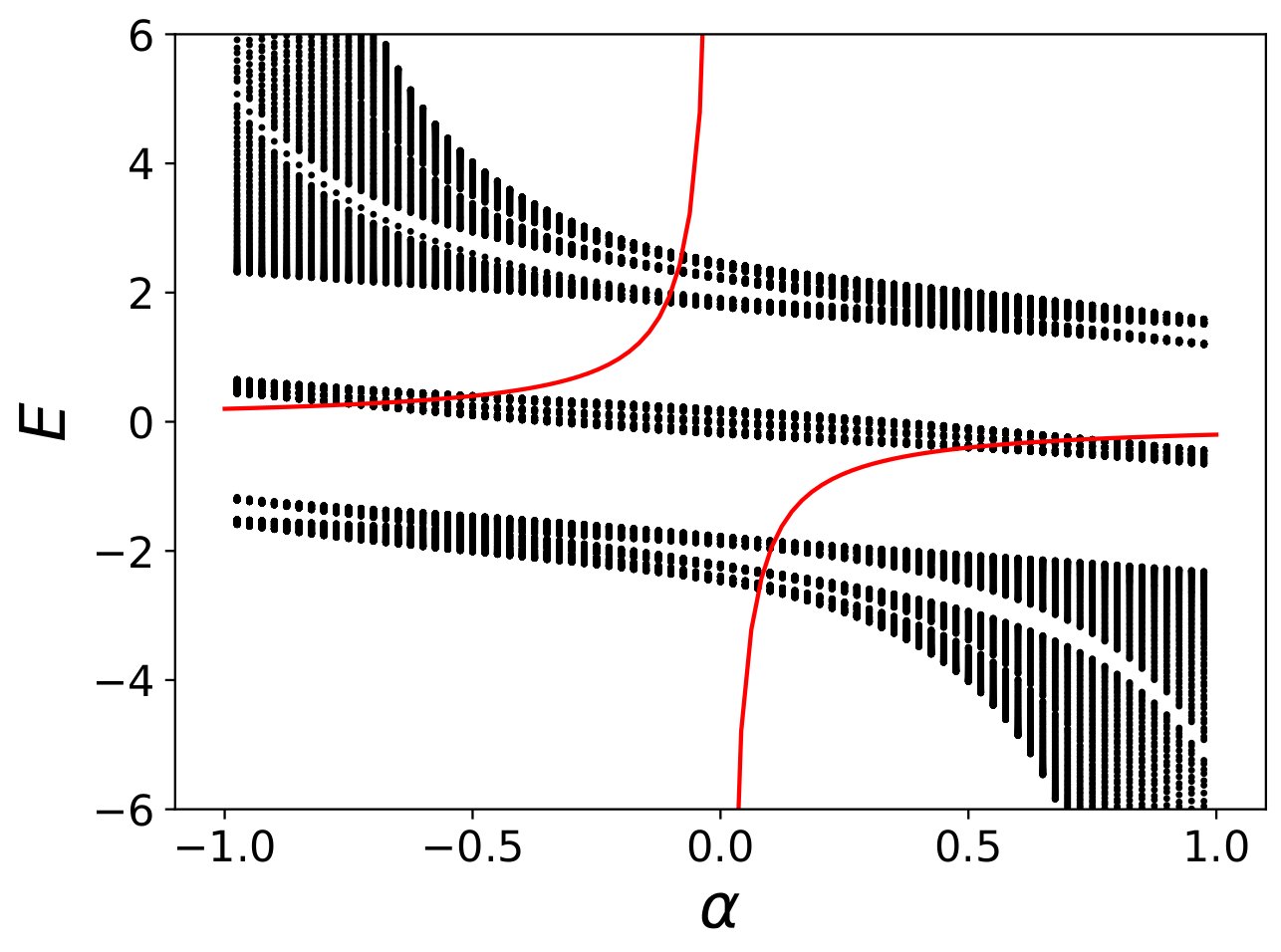
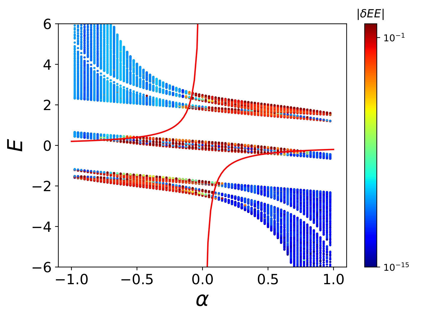
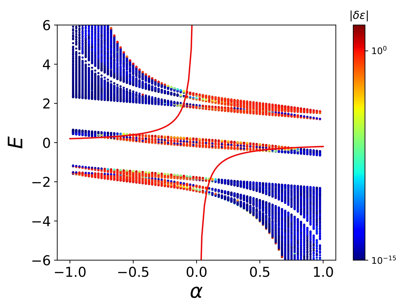
Figure 5: (color online) Left panel: spectrum of the Hamiltonian of Eq. (6) with the on-site energies of Eq. (7). The mobility edges which are determined by Eq. (8) are plotted in red. Middle panel: magnitude of shift in the entanglement entropy $|\delta EE|$ when boundary condition changes from PBC to APBC for the whole spectrum and for $\alpha$ between $-1$ and $1$. Right panel: magnitude of Shift in the smallest magnitude entanglement energy $|\delta\epsilon|$. $N=500$. Colorbars are plotted in log scale.

IV Concluding Remarks

We examined the effect of the change in the boundary conditions on the entanglement properties of the system. Namely, we changed the boundary conditions from PBC to APBC and studied the change in the spectrum of the entanglement Hamiltonian and also in the entanglement entropy. By using one-dimensional free fermion models which have LD phase transition, we showed numerically that in the delocalized phase the spectrum of the entanglement Hamiltonian and thus entanglement entropy changes, but in the localized phase the shift is negligible. We also studied the shift in one of the eigen-values of the entanglement Hamiltonian, the smallest magnitude entanglement energy, and we showed that this shift is enough to determine the phase transition point: shift $|\delta\epsilon|$ is non-zero in the delocalized phase and sharply goes to zero in localized phase. Thus we verified that the shift in the entanglement Hamiltonian spectrum can be identified as a new phase detection parameter.

We studied the LD phase transition by examining the ground state entanglement Hamiltonian instead of original Hamiltonian of the system. The next question would be: can we obtain the conductance properties of the system by examining the entanglement Hamiltonian rather than Hamiltonian of the system? In addition, $\delta\epsilon$ as a phase detection parameter, deserves more studies for models with randomness. For example it is interesting to study $\delta\epsilon$ and its distribution in two and three-dimensional Anderson models with weak localization and localization-delocalization phase transitions. Clearly, such issues would be of interest and we intend to address these in the future.

- (1) R. Horodecki, P. Horodecki, M. Horodecki, and K. Horodecki, Rev. Mod. Phys. 81, 865 (2009).
- (2) M. A. Nielsen, I. L. Chuang, Quantum Computation and Quantum Information (Cambridge University Press) (Cambridge) (2010).
- (3) A. Ekert, Phys. Rev. Lett 67, 661 (1991).
- (4) A. Steane, Rep. Prog. Phys. 61, 117 (1998).
- (5) N. Gisin, G. Ribordy, W. Tittel, and H. Zbinden, Rev. Mod. Phys. 74, 145 (2002).
- (6) A. Osterloh, L. Amico, G. Falci, R. Fazio, Nature 416, 608-610 (2002).
- (7) L. Amico, R. Fazio, A. Osterloh, and V. Vedral, Rev. Mod. Phys. 80, 517 (2008).
- (8) M. Haque, O. Zozulya, and K. Schoutens, Phys. Rev. Lett. 98, 060401 (2007).
- (9) A. Kitaev and J. Preskill, Phys. Rev. Lett. 96, 110404 (2006).
- (10) A. Chandran, V. Khemani, and S. L. Sondhi, Phys. Rev. Lett. 113, 060501 (2014).
- (11) Min-Fong Yang, Phys. Rev. A 71, 030302(R) (2005).
- (12) V. Vedral, M. B. Plenio, M. A. Rippin, and P. L. Knight, Phys. Rev. Lett. 78, 2275 (1997).
- (13) G. Vidal, J. I. Latorre, E. Rico, and A. Kitaev, Phys. Rev. Lett. 90, 227902 (2003).
- (14) T. J. Osborne and M. A. Nielsen, Phys. Rev. A 66, 032110 (2002).
- (15) S. J. Gu, S. S. Deng, Y. Q. Li, and H. Q. Lin, Phys. Rev. Lett. 93, 086402 (2004).
- (16) J. Vidal, G. Palacios, and R. Mosseri, Phys. Rev. A 69, 022107 (2004).
- (17) I. Mondragon-Shem, M. Khan, and T. L. Hughes, Phys. Rev. Lett. 110, 046806 (2013).
- (18) E. C. Andrade, M. Steudtner, M. Vojta, J. Stat. Mech. P07022 (2014) .
- (19) I. Mondragon-Shem and T. L. Hughes, Phys. Rev. B 90, 104204 (2014).
- (20) M. Legner and T. Neupert, Phys. Rev. B 88, 115114 (2013). O. S. Zozulya, M. Haque, K. Schoutens, and E. H. Rezayi, Phys. Rev. B 76, 125310 (2007). M. C. Arnesen, S. Bose, and V. Vedral, Phys. Rev. Lett.87, 017901 (2001). Ronny Thomale, D. P. Arovas, and B. A. Bernevig, Phys. Rev. Lett. 105, 116805 ( 2010).
- (21) T. C. Wei, D. Das, S. Mukhopadyay, S. Vishveshwara, and P. M. Goldbart Phys. Rev. A 71 060305(R) (2005).
- (22) P. J. Love, A.M. van den Brink, A.Y. Smirnov, et al. Quantum Inf Process 6:187 (2007).
- (23) R. W. Chhajlany, P. Tomczak, A. Wojcik, and J. Richter Phys. Rev. A 75, 032340 (2007).
- (24) A. Montakhab and A. Asadian, Phys. Rev. A 77, 062322 (2008).
- (25) A. Montakhab and A. Asadian, Phys. Rev. A 82, 062313 (2010).
- (26) H. Li and F. D. M. Haldane, Phys. Rev. Lett. 101, 010504 (2008).
- (27) M. Pouranvari, K. Yang, Phys. Rev. B 88, 075123 (2013).
- (28) M. Pouranvari, K. Yang, Phys. Rev. B 89, 115104 (2014).
- (29) M. Pouranvari, K. Yang, Phys. Rev. B 92, 245134 (2015).
- (30) R. Berkovits, Phys. Rev. Lett. 115, 206401 (2015).
- (31) S. Chakravarty, Int. J. Mod. Phys. B 24, 1823 (2010).
- (32) A. Zhao, R. L. Chu, S. Q. Shen, Phys. Rev. B 87, 205140 (2013).
- (33) M. Pouranvari, Y. Zhang, K. Yang, Advances in Condensed Matter Physics, vol. 2015, 397630 (2015).
- (34) R. Berkovits, Phys. Rev. Lett. 108, 176803 (2012).
- (35) J. H. Bardarson, F. Pollmann, and J. E. Moore, Phys. Rev. Lett. 109, 017202 (2012).
- (36) S. Nag, A. Garg, arXiv:1701.00236.
- (37) J. L. C. da C. Filho, A. Saguia, L. F. Santos, M. S. Sarandy, arXiv:1705.01957.
- (38) S. D. Geraedts, N. Regnault, R. M. Nandkishore, arXiv:1705.00631.
- (39) V. Khemani, S. P. Lim, D. N. Sheng, and D. A. Huse, Phys. Rev. X 7, 021013 (2017).
- (40) Z. Yang, A. Hamma, S. M. Giampaolo, E. R. Mucciolo, C. Chamon, arXiv:1703.03420.
- (41) R. Berkovits, Ann. Phys. (Berlin), 1700042 (2017).
- (42) L. Vidmar, L. Hackl, E. Bianchi, and M. Rigol, arXiv:1703.02979.
- (43) N. Laflorencie, E. S. Sorensen, M. S. Chang, and I. Affleck, Phys. Rev. Lett.96, 100603 (2006).
- (44) G. C. Levine, Phys. Rev. Lett. 93, 266402 (2004).
- (45) I. Peschel, J. Phys. A: Math. Gen. 38 4327 (2005).
- (46) B. I. Shklovskii, B. Shapiro, B. R. Sears, P. Lambrianides, and H. B. Shore, Phys. Rev. B 47, 11487 (1993).
- (47) J. T. Edwards and D. J. Thouless, J. Phys. C: Solid State Phys., Vol. 5 (1972).
- (48) P.W. Anderson, D. J. Thouless, E. Abrahams, D. S. Fisher, Phys. Rev. B 22, 3519, (1980).
- (49) E. N. Economou and C. M. Soukoulis, Phys. Rev. Lett. 46, 618 (1981).
- (50) B. Kramer, A. MacKinnon, Rep. Prog. Phys. 56 1469-1564 (1993).
- (51) for a description of the look at Ref. [ref:pouranvariyang2, ]
- (52) R. B. Diener, G. A. Georgakis, J. Zhong, M. Raizen, and Q. Niu, Phys. Rev. A 64, 033416 (2001).
- (53) Y. Lahini, R. Pugatch, F. Pozzi, M. Sorel, R. Morandotti, N. Davidson, and Y. Silberberg, Phys. Rev. Lett. 103, 013901 (2009).
- (54) I. Peschel, J. Phys. A: Math. Gen. 36, L205 (2003).
- (55) D. H. Dunlap, H-L. Wu, and P. W. Phillips, Phys. Rev. Lett 65, 88 (1990).
- (56) Sriram Ganeshan, J. H. Pixley, and S. Das Sarma, Phys. Rev. L. 114, 146601 (2015)
- (57) S. Aubry, G. André, Ann. Israel. Phys. Soc. 3, 133 (1980).