On the restricted almost unbiased Liu estimator in the Logistic regression model

Abstract

It is known that when the multicollinearity exists in the logistic regression model, variance of maximum likelihood estimator is unstable. As a remedy, in the context of biased shrinkage ridge estimation, Chang (2015) introduced an almost unbiased Liu estimator in the logistic regression model. Making use of his approach, when some prior knowledge in the form of linear restrictions are also available, we introduce a restricted almost unbiased Liu estimator in the logistic regression model. Statistical properties of this newly defined estimator are derived and some comparison result are also provided in the form of theorems. A Monte Carlo simulation study along with a real data example are given to investigate the performance of this estimator.

1 Introduction

Consider the following logistic regression model

$$y_{i}=\pi_{i}+\varepsilon_{i},\ i=1,\ldots,n,$$ (1)

where

$$\pi_{i}=\mbox{Pr}(y_{i}=1)=\frac{exp(x_{i}^{\prime}\beta)}{1+exp(x_{i}^{\prime}\beta)},\ i=1,2,\ldots,n$$ (2)

is the expectation of $y_{i}$ when the ith value of the dependent variable is Bernoulli with parameter $\pi_{i}$, $\beta=(\beta_{0},\beta_{1},\ldots,\beta_{p})^{\prime}$ denotes the unknown $(p+1)$-vector of regression coefficients, $x_{i}=(1,x_{1i},x_{2i},\ldots,x_{pi})^{\prime}$ denotes the ith row of $X$, the $n\times(p+1)$ data matrix, and $\varepsilon_{i}$s are independent random errors, each having zero mean and variance $w_{i}=\pi_{i}(1-\pi_{i})$.

In the estimation process of coefficient $\beta$, one often uses the maximum likelihood (ML) approach. Making use of the iteratively weighted least squares algorithm, the MLE is obtained as

$$\hat{\beta}_{MLE}=(X^{\prime}\hat{W}X)^{-1}X^{\prime}\hat{W}Z,$$ (3)

where $Z=(Z_{1},\ldots,Z_{n})^{\prime}$, with $Z_{i}=\log(\hat{\pi}_{i})+\frac{y_{i}-\hat{\pi}_{i}}{\hat{\pi}_{i}(1-\hat{\pi}_{i})}$ and $\hat{W}=\mbox{Diag}(\hat{\pi}_{i}(1-\hat{\pi}_{i}))$.

In the context of linear regression model, when the multicollinearity exists, the ordinary least squares (OLS) estimator is no longer an efficient estimator. To overcome the problem of multicollinearity, new biased shrinkage estimators have been proposed. As such, Liu (1993) proposed the Liu estimator, the almost unbiased Liu estimator proposed by Akdeniz and Kaçıranlar (1995), the restricted Liu estimator proposed by Kaçıranlar et al. (1999), the restricted almost unbiased Liu estimator introduced by Xu and Yang (2011a,b) and more recently Asar et al. (2015) developed a two-parameter restricted Liu estimator.

In the logistic regression model, when the explanatory variables are highly correlated, the variance of the MLE becomes inflated. Dealing with such a problem, some estimators are proposed. One of them is the ridge estimator of Schaefer et al. (1984). When some prior information, in the form of restrictions on regression coefficients, are available, Duffy and Santner (1989) suggested to use the restricted MLE (RMLE).

Now, suppose we are provided with some prior information about $\beta$ in the form of linear restrictions

$$H\beta=h,$$ (4)

where $H$ is a $q\times(p+1)$ ($q\leq p+1$) known matrix and $h$ denotes a $q\times 1$ vector of pre-specified known constants.

Considering such a case, Duffy and Santner (1989) defined the RMLE given by

$$\hat{\beta}_{RMLE}=\hat{\beta}_{MLE}-C^{-1}H^{\prime}(HC^{-1}H^{\prime})^{-1}(H\hat{\beta}_{MLE}-h),$$ (5)

where $C=X^{\prime}\hat{W}X$.

Mansson et al. (2011) defined the Liu estimator (LE) of $\beta$ in the logistic regression model given by

$$\hat{\beta}_{LE}=(C+I)^{-1}(C+dI)\hat{\beta}_{MLE},$$ (6)

where $0<d<1$ is the biasing parameter.

Şiray et al. (2015) combined the LE and RMLE, to introduce a restricted Liu estimator (RLE) in the logistic regression model as follows

$$\hat{\beta}_{RLE}=(C+I)^{-1}(C+dI)\hat{\beta}_{RMLE},$$ (7)

where $0<d<1$ is the biasing parameter.

In order to reduce the bias of LE, Chang (2015) proposed an almost unbiased Liu estimator (AULE) which has form

$$\hat{\beta}_{AULE}=[I-(1-d)^{2}(C+I)^{-2}]\hat{\beta}_{MLE}$$ (8)

In this paper, using the latter result, a restricted almost unbiased Liu estimator will be exhibited in the logistic regression model when both multicollinearity and restrictions are present.

We organize the paper as follows: Section 2 contains the introduction of the new estimator along with some preliminary lemmas. Comparisons between this estimator with other existing ones are considered in section 3, while a numerical example is conducted in section 4. The work is concluded in section 5.

2 Proposed Estimator

In the same fashion as in Şiray et al. (2015), the AULE and RLE will be combined to obtain a new estimator namely restricted almost unbiased Liu estimator (RAULE) with form

$$\hat{\beta}_{RAULE}=[I-(1-d)^{2}(C+I)^{-2}]\hat{\beta}_{RMLE},$$ (9)

where $C=X^{\prime}\hat{W}X$ and $0<d<1$ is the biasing parameter.
Letting $L_{d}=[I-(1-d)^{2}(C+I)^{-2}]$, the RAULE can be expressed as

$$\hat{\beta}_{RAULE}=L_{d}\hat{\beta}_{RMLE}.$$ (10)

For comparison sake and in order to derive characteristics of the RAULE, we need the following lemmas.

Lemma 2.1. (Shi, 2001) Under the assumptions of section 1, the following matrix is nonnegative definite and has rank $p+1-q$.

$$A=C^{-1}-C^{-1}H^{\prime}(HC^{-1}H^{\prime})^{-1}HC^{-1}$$

Lemma 2.2. (Baksalary and Kala, 1983) Suppose that $M$ be a nonnegative definite matrix and $\alpha$ be a vector, then

$$M-\alpha\alpha^{\prime}\geq 0\Leftrightarrow\alpha^{\prime}M^{+}\alpha\leq 1,\ \alpha\in\Re(M)$$

where $M^{+}$ denotes the Moore-Penrose inverse of $M$.

Lemma 2.3.(Wang, 1994) Suppose that $M$ be a positive definite matrix and $N$ be a nonnegative definite matrix, then

$$M-N\geq 0\Leftrightarrow\lambda_{max}(NM^{-1})\leq 1$$

Lemma 2.4.(Wang, 1994) Suppose that both $M$ and $N$ are nonnegative definite matrices, then

$$M-N\geq 0\Leftrightarrow\lambda_{max}(NM^{-})\leq 1,\ \Re(N)\subset\Re(M)$$

where $\lambda_{max}(NM^{-})\leq 1$ is invariant of the choice of $M^{-}$, and $M^{-}$ stands for the generalized inverse of $M$.

In the forthcoming section, we will be deriving some properties of the proposed estimator and compare it with some existing competitors.

3 Properties & Comparison

Let $\hat{\theta}$ be an estimator of the parameter $\theta$. The matrix mean squared error (MMSE) of $\hat{\theta}$ is defined by

$$MMSE(\hat{\theta})=E(\hat{\theta}-\theta)(\hat{\theta}-\theta)^{\prime}=Cov(\hat{\theta})+Bias(\hat{\theta})Bias(\hat{\theta})^{\prime},$$ (11)

where $Cov(\cdot)$ is the covariance matrix and

$$Bias(\hat{\theta})=E(\hat{\theta})-\theta.$$

The scalar mean squared error (MSE) of $\hat{\theta}$ is defined as

$$MSE(\hat{\theta})=\mbox{tr}[MMSE(\hat{\theta})]=\mbox{tr}(Cov(\hat{\theta}))+Bias(\hat{\theta})^{\prime}Bias(\hat{\theta}).$$ (12)

For two given estimators $\hat{\theta}_{1}$ and $\hat{\theta}_{2}$ of $\theta$, the estimator $\hat{\theta}_{2}$ is said to be superior to estimator $\hat{\theta}_{1}$ in the sense of MMSE criterion, if and only if

$$\Delta(\hat{\theta}_{1},\hat{\theta}_{2})=MMSE(\hat{\theta}_{1})-MMSE(\hat{\theta}_{2})\geq 0$$ (13)

Now, we derive the MMSE of the new estimator (RAULE).

Proposition 3.1. Under the assumptions of the logistic regression model (1), when the restrictions (4) hold, the MMSE of the new estimator is given by

$$MMSE(\hat{\beta}_{RAULE}) = L_{d}AL_{d}+\beta^{\prime}(L_{d}-I)^{\prime}(L_{d}-I)\beta,$$ (14)

where $A=C^{-1}-C^{-1}H^{\prime}(HC^{-1}H^{\prime})^{-1}HC^{-1}$.
Proof: Using Eq. (9), the covariance and bias of the new estimator are respectively evaluated as

$$Cov(\hat{\beta}_{RAULE})=L_{d}AL_{d}$$ (15)

$$Bias(\hat{\beta}_{RAULE})=(L_{d}-I)\beta$$ (16)

Then we obtain

$$MMSE(\hat{\beta}_{RAULE}) = L_{d}AL_{d}+\beta^{\prime}(L_{d}-I)^{\prime}(L_{d}-I)\beta$$ (17)

Lemma 3.2. Under the assumptions of the logistic regression model (1), MMSE of the MLE, AULE and RMLE are respectively given by

$$MMSE(\hat{\beta}_{MLE})=C^{-1}$$ (18)

$$MMSE(\hat{\beta}_{AULE})=L_{d}C^{-1}L_{d}+\beta^{\prime}(L_{d}-I)^{\prime}(L_{d}-I)\beta$$ (19)

$$MMSE(\hat{\beta}_{RMLE})=ACA$$ (20)

In the following result, we will be presenting the necessary and sufficient conditions for the new estimator to be superior to the RMLE in the MMSE sense.

Theorem 3.3. Under the assumptions of the logistic regression model (1), assume $\lambda_{max}(L_{d}AL_{d}(ACA)^{-})\leq 1$ and $\Re(L_{d}AL_{d})\in\Re(ACA)$. Then, the RAULE is superior to the RMLE in the MMSE sense if and only if

$$b_{1}^{\prime}(ACA-L_{d}AL_{d})^{+}b_{1}\leq 1,\quad b_{1}\in\Re(ACA-L_{d}AL_{d}),$$ (21)

where $b_{1}=(L_{d}-I)\beta$.
Proof: The difference in MMSE is given by

$$\Delta_{1} = MMSE(\hat{\beta}_{RMLE})-MMSE(\hat{\beta}_{RAULE})$$ (22)

$$= ACA-L_{d}AL_{d}-b_{1}b_{1}^{\prime}.$$ (23)

Since $ACA\geq 0$ and $L_{d}AL_{d}\geq 0$, making use of Lemma 2.4, under the given assumptions, one obtains $ACA-L_{d}AL_{d}\geq 0$. Then, the result follows by applying Lemma 2.2.

Now, necessary and sufficient conditions for the new estimator to be superior to the RMLE in the MSE sense, will be given.

Theorem 3.4. Under the assumptions of the logistic regression model (1), the RAULE is superior to the RMLE in the MSE sense, if the biasing parameter $d$ satisfies the following inequality

$$\frac{(\lambda_{1}+d)(\lambda_{1}+2-d)}{(1-d)^{2}}<\frac{max_{i}\alpha_{i}^{2}}{min_{i}a_{ii}},$$

where $\lambda_{1}\geq\ldots\geq\lambda_{p+1}$ are the ordered eigenvalues of $C$, $a_{ii}\geq 0$ is the ith diagonal element of the matrix $T^{\prime}AT$ and $\alpha_{i}$ is the ith elements of $\beta^{\prime}T$ for the orthogonal matrix $T$.
Proof. Consider the MSE difference

$$\Delta_{2} = MSE(\hat{\beta}_{RMLE})-MSE(\hat{\beta}_{RAULE})$$ (24)

$$= tr[MMSE(\hat{\beta}_{RMLE})-MMSE(\hat{\beta}_{RAULE})]$$ (25)

$$= \sum_{i=1}^{p+1}\frac{1}{(\lambda_{i}+1)^{4}}[(\lambda_{i}+2-d)^{2}(\lambda_{i}+d)^{2}-(\lambda_{i}+1)^{4}]a_{ii}+(1-d)^{4}\alpha_{i}^{2}].$$ (26)

Differentiating $\Delta_{2}$ with respect to $d$, gives

$$\frac{\partial\Delta_{2}}{\partial d} = \sum_{i=1}^{p+1}\frac{(1-d)^{3}}{(\lambda_{i}+1)^{4}}\left[\frac{4(\lambda_{i}+d)(\lambda_{i}+2-d)a_{ii}}{(1-d)^{2}}-4\alpha_{i}^{2}\right]$$ (27)

$$\leq \sum_{i=1}^{p+1}\frac{4(1-d)^{3}}{(\lambda_{i}+1)^{4}}\left[\frac{(\lambda_{1}+d)(\lambda_{1}+2-d)min_{i}a_{ii}}{(1-d)^{2}}-max_{i}\alpha_{i}^{2}\right].$$

The result follows whenever

$$\frac{(\lambda_{1}+d)(\lambda_{1}+2-d)}{(1-d)^{2}}<\frac{max_{i}\alpha_{i}^{2}}{min_{i}a_{ii}}.$$

Now, we give comparison result between the RAULE and MLE in the MMSE sense.
Theorem 3.5. Under the assumptions of the logistic regression model (1), when $\lambda_{max}(L_{d}AL_{d}C)\leq 1$, RAULE is superior to the MLE in the MMSE sense if and only if

$$b_{1}^{\prime}(C^{-1}-L_{d}AL_{d})^{+}b_{1}\leq 1,\quad b_{1}\in\Re(C^{-1}-L_{d}AL_{d}),$$ (28)

where $b_{1}=(L_{d}-I)\beta$.
Proof. The difference in MMSE is given by

$$\Delta_{3} = MMSE(\hat{\beta}_{MLE})-MMSE(\hat{\beta}_{RAULE})$$ (29)

$$= C^{-1}-L_{d}AL_{d}-b_{1}b_{1}^{\prime}.$$ (30)

Since $C^{-1}>0$ and $L_{d}AL_{d}\geq 0$, applying Lemma 2.3 yields $C^{-1}-L_{d}AL_{d}\geq 0$. Then the result follows applying Lemma 2.2.

Theorem 3.6. Under the assumptions of the logistic regression model (1), when

$$\frac{(\lambda_{1}+d)(\lambda_{1}+2-d)}{(1-d)^{2}}<\frac{max_{i}\alpha_{i}^{2}}{min_{i}a_{ii}},$$

the RAULE is superior to MLE in the sense of MSE criterion.

Proof. Consider the MSE difference given by

$$\Delta_{4} = MSE(\hat{\beta}_{MLE})-MSE(\hat{\beta}_{RAULE})$$ (31)

$$= \mbox{tr}[MMSE(\hat{\beta}_{MLE})-MMSE(\hat{\beta}_{RAULE})]$$ (32)

$$= \mbox{tr}[MMSE(\hat{\beta}_{MLE})-MMSE(\hat{\beta}_{RMLE})$$ (34)

$$+MMSE(\hat{\beta}_{RMLE})-MMSE(\hat{\beta}_{RAULE})].$$

Since

$$\mbox{tr}[MMSE(\hat{\beta}_{MLE})-MMSE(\hat{\beta}_{RMLE})] = \mbox{tr}[C^{-1}-ACA]$$

$$= \mbox{tr}[C^{-1}-A]$$

$$= \mbox{tr}[C^{-1}H^{\prime}(HC^{-1}H^{\prime})^{-1}HC^{-1}]\geq 0$$

we have $\mbox{tr}[MMSE(\hat{\beta}_{RMLE})-MMSE(\hat{\beta}_{MAULE})]\geq 0$. Hence $\Delta_{4}\geq 0$, using Theorem 3.4.

Finally we present the comparison between the RAULE and AULE in the MMSE sense.
Theorem 3.7. Under the assumptions of the logistic regression model (1), the RAULE is always superior to AULE in the MMSE sense.
Proof. Consider the following difference in MMSE

$$\Delta_{5} = MMSE(\hat{\beta}_{AULE})-MMSE(\hat{\beta}_{RAULE})$$ (35)

$$= L_{d}C^{-1}L_{d}-L_{d}AL_{d}$$ (36)

$$= L_{d}(C^{-1}-A)L_{d}.$$ (37)

Making use of Lemma 2.1, $C^{-1}-A=C^{-1}H^{\prime}(HC^{-1}H^{\prime})^{-1}HC^{-1}\geq 0$ and the proof is complete.

Corollary 3.1. The RAULE is always superior to the AULE in the MSE sense.

4 Monte Carlo Simulation

4.1 The design of the simulation

In this section, we conduct a Monte Carlo simulation to compare the performances of the MLE, AULE, RMLE and RAULE under different scenarios. Since we want to compare the estimators when there multicollinearity is present, the main factor of the simulation is the degree of correlation $\left(\rho^{2}\right)$ among the explanatory variables. Hence, following Gibbons (1981) and Kibria (2003), we use the following formula to generate correlated variables:

$$x_{ij}=(1-\rho^{2})^{1/2}z_{ij}+\rho z_{ip},\ i=1,...,n,\ j=1,...,p,$$ (38)

where $z_{ij}$s are independent standard normal pseudo-random numbers. We consider three different values of the degree of correlation corresponding to $0.9,0.99$ and $0.999$.

The number of $n$ observations is generated using the Bernoulli distribution with parameter $\pi_{i}$ such that

$$\pi_{i}=\frac{exp(x_{i}^{\prime}\beta)}{1+exp(x_{i}^{\prime}\beta)},\ i=1,2,\ldots,n,$$ (39)

for the dependent variable.

We fit logistic regression models having $p=4$ and $p=8$ explanatory variables. We consider the sample sizes $50,100$ and $200$. The parameter values of $\beta$ are chosen so that $\beta^{\prime}\beta=1$.

Following Månsson et al. (2015), we use different restriction matrices, to capture the effect of imposing restrictions on estimators, as follows:

I) $H_{1}=\left(\begin{array}[]{cccc}1&0&-2&1\\ 1&-1&1&-1\\ \end{array}\right)$ with $h_{1}=(0,0)^{\prime}$ when $p=4$ and

II) $H_{2}=\left(\begin{array}[]{cccccccc}1&0&-2&1&-3&1&1&1\\ 1&1&0&1&-3&1&-2&1\\ \end{array}\right)$ with $h_{2}=(0,0)^{\prime}$ when $p=8$.
The simulation is replicated $2000$ times and estimated MSE is evaluated using

$$\mbox{MSE}=\frac{\sum_{r=1}^{2000}(\tilde{\beta}_{r}-\beta)^{\prime}(\tilde{\beta}_{r}-\beta)}{2000},$$

where $\tilde{\beta}_{r}$ is any estimator considered in this study, in the rth repetition.

4.2 Results of the simulation

We summarized the estimated MSE values of the estimators in Tables 1-6. It can be observed that an increase in the degree of correlation affects the MSE values of the estimators negatively. It is also observed that MSE has the worst performance (having the most MSE values) in all of the situations considered. The RMLE has always less MSE than that of MLE.

The performances of the AULE and RAULE depend on the parameter $d$. The smaller the value of $d$, the better performance. The RMLE has lesser MSE value than AULE when $d>0.4$ in almost all cases.

Moreover, it can be deduced that our new estimator RAULE has always the least MSE value. Especially, the RAULE is the most robust option against the correlation when the value of $d$ is small.

From tables, it is realized that an increase in the sample size causes a decrease in the MSE values. Increasing the number of explanatory variables also affects the performances of the estimator negatively. Again the newly proposed RAULE is the most robust option for this situation.

Table 1: The estimated MSE values for different $d$ when $n=50$ and $p=4$

	$d=0.1$	$d=0.2$	$d=0.3$	$d=0.4$	$d=0.5$	$d=0.6$	$d=0.7$	$d=0.8$	$d=0.9$	$d=0.99$
$\gamma=0.9$
MLE	14.6207	14.6207	14.6207	14.6207	14.6207	14.6207	14.6207	14.6207	14.6207	14.6207
AULE	2.4696	4.0121	5.8178	7.7198	9.5737	11.2573	12.6704	13.7354	14.3966	14.6185
RMLE	3.3376	3.3376	3.3376	3.3376	3.3376	3.3376	3.3376	3.3376	3.3376	3.3376
RAULE	0.9280	1.2590	1.6281	2.0065	2.3691	2.6946	2.9658	3.1692	3.2950	3.3372
$\gamma=0.99$
MLE	122.8774	122.8774	122.8774	122.8774	122.8774	122.8774	122.8774	122.8774	122.8774	122.8774
AULE	6.3439	18.3859	34.4887	52.5983	70.9343	87.9906	102.5346	113.6079	120.5258	122.8537
RMLE	17.6015	17.6015	17.6015	17.6015	17.6015	17.6015	17.6015	17.6015	17.6015	17.6015
RAULE	1.4451	3.2122	5.4877	8.0031	10.5255	12.8580	14.8392	16.3440	17.2826	17.5983
$\gamma=0.999$
MLE	2988.9881	2988.9881	2988.9881	2988.9881	2988.9881	2988.9881	2988.9881	2988.9881	2988.9881	2988.9881
AULE	109.4131	389.4573	779.6334	1226.2873	1682.9183	2110.1799	2475.8795	2754.9782	2929.5914	2988.3912
RMLE	279.7609	279.7609	279.7609	279.7609	279.7609	279.7609	279.7609	279.7609	279.7609	279.7609
RAULE	10.7511	37.0637	73.5805	115.3140	157.9420	197.8068	231.9161	257.9424	274.2231	279.7052

Table 2: The estimated MSE values for different $d$ when $n=100$ and $p=4$

	$d=0.1$	$d=0.2$	$d=0.3$	$d=0.4$	$d=0.5$	$d=0.6$	$d=0.7$	$d=0.8$	$d=0.9$	$d=0.99$
$\gamma=0.9$
MLE	5.7257	5.7257	5.7257	5.7257	5.7257	5.7257	5.7257	5.7257	5.7257	5.7257
AULE	2.5062	3.0270	3.5549	4.0642	4.5327	4.9417	5.2757	5.5229	5.6746	5.7252
RMLE	1.7583	1.7583	1.7583	1.7583	1.7583	1.7583	1.7583	1.7583	1.7583	1.7583
RAULE	1.1074	1.2195	1.3292	1.4325	1.5259	1.6063	1.6714	1.7192	1.7484	1.7582
$\gamma=0.99$
MLE	50.0384	50.0384	50.0384	50.0384	50.0384	50.0384	50.0384	50.0384	50.0384	50.0384
AULE	4.2987	9.4622	15.9754	23.1044	30.2129	36.7629	42.3141	46.5238	49.1475	50.0294
RMLE	9.8945	9.8945	9.8945	9.8945	9.8945	9.8945	9.8945	9.8945	9.8945	9.8945
RAULE	1.5374	2.5562	3.7795	5.0856	6.3692	7.5410	8.5281	9.2737	9.7373	9.8929
$\gamma=0.999$
MLE	461.9003	461.9003	461.9003	461.9003	461.9003	461.9003	461.9003	461.9003	461.9003	461.9003
AULE	18.9701	62.9223	123.3250	192.0703	262.1311	327.5616	383.4969	426.1535	452.8284	461.8091
RMLE	124.0645	124.0645	124.0645	124.0645	124.0645	124.0645	124.0645	124.0645	124.0645	124.0645
RAULE	5.5594	17.3608	33.5400	51.9347	70.6708	88.1627	103.1129	114.5124	121.6405	124.0402

Table 3: The estimated MSE values for different $d$ when $n=200$ and $p=4$

	$d=0.1$	$d=0.2$	$d=0.3$	$d=0.4$	$d=0.5$	$d=0.6$	$d=0.7$	$d=0.8$	$d=0.9$	$d=0.99$
$\gamma=0.9$
MLE	2.4237	2.4237	2.4237	2.4237	2.4237	2.4237	2.4237	2.4237	2.4237	2.4237
AULE	1.8950	1.9963	2.0899	2.1743	2.2481	2.3100	2.3592	2.3949	2.4165	2.4237
RMLE	1.1825	1.1825	1.1825	1.1825	1.1825	1.1825	1.1825	1.1825	1.1825	1.1825
RAULE	1.0220	1.0532	1.0818	1.1074	1.1297	1.1484	1.1632	1.1739	1.1803	1.1825
$\gamma=0.99$
MLE	18.7164	18.7164	18.7164	18.7164	18.7164	18.7164	18.7164	18.7164	18.7164	18.7164
AULE	3.4884	5.5229	7.8305	10.2190	12.5219	14.5982	16.3327	17.6356	18.4430	18.7137
RMLE	4.8649	4.8649	4.8649	4.8649	4.8649	4.8649	4.8649	4.8649	4.8649	4.8649
RAULE	1.4912	1.9655	2.4871	3.0174	3.5228	3.9750	4.3508	4.6321	4.8061	4.8643
$\gamma=0.999$
MLE	168.3497	168.3497	168.3497	168.3497	168.3497	168.3497	168.3497	168.3497	168.3497	168.3497
AULE	8.5172	24.9718	47.0305	71.8658	97.0272	120.4414	140.4116	155.6186	165.1198	168.3173
RMLE	52.5252	52.5252	52.5252	52.5252	52.5252	52.5252	52.5252	52.5252	52.5252	52.5252
RAULE	3.0800	8.1803	15.0086	22.6921	30.4739	37.7139	43.8883	48.5895	51.5267	52.5151

Table 4: The estimated MSE values for different $d$ when $n=50$ and $p=8$

	$d=0.1$	$d=0.2$	$d=0.3$	$d=0.4$	$d=0.5$	$d=0.6$	$d=0.7$	$d=0.8$	$d=0.9$	$d=0.99$
$\gamma=0.9$
MLE	141.9664	141.9664	141.9664	141.9664	141.9664	141.9664	141.9664	141.9664	141.9664	141.9664
AULE	8.3150	22.3253	40.8815	61.6607	82.6499	102.1456	118.7542	131.3918	139.2840	141.9395
RMLE	42.1899	42.1899	42.1899	42.1899	42.1899	42.1899	42.1899	42.1899	42.1899	42.1899
RAULE	3.5096	7.7610	13.2181	19.2412	25.2760	30.8532	35.5891	39.1851	41.4281	42.1823
$\gamma=0.99$
MLE	1270.2249	1270.2249	1270.2249	1270.2249	1270.2249	1270.2249	1270.2249	1270.2249	1270.2249	1270.2249
AULE	48.8557	168.8119	334.8236	524.3276	717.7695	898.6031	1053.2906	1171.3026	1245.1183	1269.9726
RMLE	368.8009	368.8009	368.8009	368.8009	368.8009	368.8009	368.8009	368.8009	368.8009	368.8009
RAULE	15.1951	50.3383	98.5839	153.4681	209.3890	261.6062	306.2416	340.2786	361.5626	368.7282
$\gamma=0.999$
MLE	46865.2930	46865.2930	46865.2930	46865.2930	46865.2930	46865.2930	46865.2930	46865.2930	46865.2930	46865.2930
AULE	1693.7814	6076.5807	12192.7161	19198.8276	26364.0035	33069.7799	38810.1409	43191.5188	45932.7934	46855.9216
RMLE	12492.1038	12492.1038	12492.1038	12492.1038	12492.1038	12492.1038	12492.1038	12492.1038	12492.1038	12492.1038
RAULE	452.1749	1620.7160	3251.0570	5118.4698	7028.1898	8815.4162	10345.3121	11513.0044	12243.5835	12489.6063

Table 5: The estimated MSE values for different $d$ when $n=100$ and $p=8$

	$d=0.1$	$d=0.2$	$d=0.3$	$d=0.4$	$d=0.5$	$d=0.6$	$d=0.7$	$d=0.8$	$d=0.9$	$d=0.99$
$\gamma=0.9$
MLE	26.2009	26.2009	26.2009	26.2009	26.2009	26.2009	26.2009	26.2009	26.2009	26.2009
AULE	4.6742	7.4254	10.6324	14.0028	17.2834	20.2599	22.7567	24.6377	25.8052	26.1969
RMLE	11.8713	11.8713	11.8713	11.8713	11.8713	11.8713	11.8713	11.8713	11.8713	11.8713
RAULE	2.7895	4.0017	5.3773	6.8017	8.1754	9.4141	10.4490	11.2264	11.7082	11.8697
$\gamma=0.99$
MLE	309.5121	309.5121	309.5121	309.5121	309.5121	309.5121	309.5121	309.5121	309.5121	309.5121
AULE	14.7981	44.9405	85.5269	131.3111	177.7461	220.9848	257.8793	285.9813	303.5420	309.4521
RMLE	141.9314	141.9314	141.9314	141.9314	141.9314	141.9314	141.9314	141.9314	141.9314	141.9314
RAULE	7.5535	21.5523	40.1706	61.0585	82.1795	101.8102	118.5408	131.2744	139.2280	141.9042
$\gamma=0.999$
MLE	3051.3774	3051.3774	3051.3774	3051.3774	3051.3774	3051.3774	3051.3774	3051.3774	3051.3774	3051.3774
AULE	113.5289	400.3017	798.8422	1254.5856	1720.2427	2155.7995	2528.5172	2812.9323	2990.8567	3050.7692
RMLE	1382.3472	1382.3472	1382.3472	1382.3472	1382.3472	1382.3472	1382.3472	1382.3472	1382.3472	1382.3472
RAULE	52.1509	182.3238	362.9193	569.2861	780.0596	977.1620	1145.8025	1274.4772	1354.9689	1382.0721

Table 6: The estimated MSE values for different $d$ when $n=200$ and $p=8$

	$d=0.1$	$d=0.2$	$d=0.3$	$d=0.4$	$d=0.5$	$d=0.6$	$d=0.7$	$d=0.8$	$d=0.9$	$d=0.99$
$\gamma=0.9$
MLE	6.6427	6.6427	6.6427	6.6427	6.6427	6.6427	6.6427	6.6427	6.6427	6.6427
AULE	3.9466	4.4224	4.8819	5.3103	5.6947	6.0240	6.2895	6.4841	6.6028	6.6423
RMLE	4.1607	4.1607	4.1607	4.1607	4.1607	4.1607	4.1607	4.1607	4.1607	4.1607
RAULE	2.6886	2.9525	3.2052	3.4393	3.6483	3.8268	3.9703	4.0752	4.1392	4.1604
$\gamma=0.99$
MLE	74.7216	74.7216	74.7216	74.7216	74.7216	74.7216	74.7216	74.7216	74.7216	74.7216
AULE	7.8025	15.6628	25.3268	35.7714	46.1097	55.5915	63.6028	69.6663	73.4407	74.7088
RMLE	39.4314	39.4314	39.4314	39.4314	39.4314	39.4314	39.4314	39.4314	39.4314	39.4314
RAULE	5.0776	9.2535	14.2768	19.6453	24.9242	29.7452	33.8072	36.8760	38.7842	39.4249
$\gamma=0.999$
MLE	815.6036	815.6036	815.6036	815.6036	815.6036	815.6036	815.6036	815.6036	815.6036	815.6036
AULE	33.8851	111.8311	218.6004	339.9454	463.5184	578.8710	677.4549	752.6211	799.6205	815.4430
RMLE	411.3009	411.3009	411.3009	411.3009	411.3009	411.3009	411.3009	411.3009	411.3009	411.3009
RAULE	18.0382	57.6046	111.4736	172.5361	234.6310	292.5449	342.0125	379.7161	403.2862	411.2203

5 Application

In this section, we present a real data application in order to show the benefit of using the newly proposed RAULE. For our purpose, we used a data set available at an official web page of Statistics Sweden (http://www.scb.se/). The observations are 83 municipalities which are the urban regions belonging to the functional analysis regions Stockholm, Malmo and Goteborg. Asar and Genc (2015) and Mansson et al. (2012) also analyzed similar data sets. We model the data using a binary logistic regression model such that the dependent variable is coded as 1 if there is an increase in the pupation and 0 if there is a decrease. The dependent variable is explained by the following explanatory variables:

X1: The population,

X2: The number of unemployed people,

X3: The number of newly constructed buildings,

X4: The number of bankrupt firms.
The correlation matrix of this data set is given in Table 7. It is observed from Table 7 that all the bivariate correlations between the explanatory variables are larger than 0.95. The condition number, being a measure of the degree of multicollinearity, is computed according to $\kappa=\sqrt{\lambda_{max}/\lambda_{min}}$ which shows that there exists a severe multicollinearity problem.

Table 7: The correlation matrix of the design matrix

	X1	X2	X3	X4
X1	1.0000	0.9937	0.9707	0.9514
X2	0.9937	1.0000	0.9527	0.9222
X3	0.9707	0.9527	1.0000	0.9765
X4	0.9514	0.9222	0.9765	1.0000

Table 8: The estimated theoretical MSE value of AULE

d	$\beta_{1}$	$\beta_{2}$	$\beta_{3}$	$\beta_{4}$	MSE
0.1	5.0078	-3.1222	0.8875	-2.0282	70.9595
0.2	9.2699	-6.1203	1.5128	-3.9040	248.9311
0.3	13.0305	-8.7656	2.0645	-5.5592	496.2849
0.4	16.2896	-11.0583	2.5427	-6.9937	779.1508
0.5	19.0474	-12.9982	2.9473	-8.2075	1068.1749
0.6	21.3038	-14.5854	3.2784	-9.2006	1338.5192
0.7	23.0587	-15.8199	3.5359	-9.9730	1569.8617
0.8	24.3122	-16.7017	3.7198	-10.5248	1746.3963
0.9	25.0644	-17.2307	3.8301	-10.8558	1856.8330
0.99	25.3126	-17.4053	3.8666	-10.9650	1894.0204

Table 9: The estimated theoretical MSE value of RAULE

d	$\beta_{1}$	$\beta_{2}$	$\beta_{3}$	$\beta_{4}$	MSE
0.1	0.5427	0.5772	0.4917	-0.8105	4.3052
0.2	0.8249	0.8521	0.7846	-1.5974	12.2573
0.3	1.0739	1.0947	1.0430	-2.2917	23.0005
0.4	1.2896	1.3050	1.2670	-2.8934	35.1374
0.5	1.4722	1.4829	1.4565	-3.4026	47.4568
0.6	1.6216	1.6284	1.6115	-3.8192	58.9338
0.7	1.7378	1.7416	1.7321	-4.1432	68.7299
0.8	1.8208	1.8225	1.8183	-4.3747	76.1930
0.9	1.8706	1.8710	1.8699	-4.5135	80.8572
0.99	1.8870	1.8870	1.8870	-4.5594	82.4270

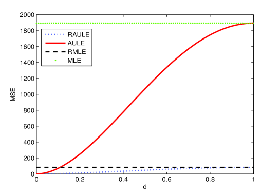
Figure 1: The estimated MSE values of the estimators when $0\leq d\leq 1$

We computed the estimated theoretical MSE values along with the coefficients of the estimators. The MSE of MLE is 1894.398 which is the largest among others. The coefficients of MLE are 25.3151, -17.4071, 3.8669 and -10.9661. The MSE of RMLE is 82.4430 and the coefficients of RMLE are 1.8872, 1.8872, 1.8872 and -4.5598. MSE values and the coefficients of AULE and RAULE are given in Tables 8 and 9 respectively for different biasing parameter $d$ varying from zero to one.

According to Tables 8-9, the RAULE has the least MSE value for all values of the parameter $d$. When $d=1$, the MSE of RAULE becomes equal to that of RMLE as expected. The MSE of AULE is lower than that of RMLE when $d<0.12$. We also provided the plot of the MSE versus $d$ in Figure 1. According to Figure 1, the RAULE has the best performance among other estimators.

6 Conclusions

In this paper, we proposed a restricted almost unbiased Liu estimator in the logistic regression model. Then, its performance compared with other competitors including the MLE, AULE, RMLE in the logistic regression model through providing some theorems, a Monte Carlo simulation as well as a real example. We concluded that our proposed estimator is superior compared to all others in the sense of having smaller MSE value.

References

- [1] Akdeniz, F. and Kaçıranlar, S. (1995). On the almost unbiased generalized Liu estimator and unbiased estimation of the bias and MSE. Comm. Statist. Theo. Meth. 24:1789-1797.
- [2] Asar, Y., Genc, A. (2015). New Shrinkage Parameters for the Liu-type Logistic Estimators. Comm. Statist. Sim. Comp.. DOI:10.1080/03610918.2014.995815.
- [3] Asar, Y., Erisoglu M. and Arashi, M. (2015). Developing a restricted two-parameter Liu-type estimator: A comparison of restricted estimators in the binary logistic regression model. Comm. Statist. Theo. Meth.. Accepted.
- [4] Baksalary, J.K., Kala, R. (1983). Partial orderings between matrices one of which is of rank one. Bull. Polish Academy Sci.. Mathematics, 31:5-7.
- [5] Duffy, D. E., Santner, T. J . (1989). On the small sample properties of norm-restricted maximum likelihood estimators for logistic regression models. Comm. Statist. Theo. Meth.. 18:959-980.
- [6] Kaçıranlar, S ., Sakalloglu, S., Akdeniz, F., Styan, G. P. H., Werner, H. J . (1999). A new biased estimator in linear regression and a detailed analysis of the widely analyzed dataset on Portland cement. Sankhya. 31:443-459.
- [7] Kibria, B . M . G. (2003). Performance of some new ridge regression estimators. Comm. Statist. Theo. Meth. 32:419-435
- [8] Liu, K. (1993). A new class of biased estimate in linear regression. Comm. Statist. Theo. Meth.. 22:393-402.
- [9] Mansson, K., Kibria, B. M. G., Shukur, G. (2011). On Liu estimators for the logit regression model. Royal Inst. Tech.(CESIS). Sweden, Paper No. 259.
- [10] Mansson, K., Kibria, B. G., Shukur, G. (2012). On Liu estimators for the logit regression model. Economic Model., 29(4):1483-1488.
- [11] Muniz, G., Kibria, B. M. G. (2009). On some ridge regression estimators: An Empirical Comparisons. Comm. Statist. Sim. Comp.. 38:621-630.
- [12] Schaefer, R . L ., Roi, L. D., Wolfe, R . A. (1984). A ridge logistic estimator. Comm. Statist. Theo. Meth.. 13:99-113.
- [13] Şiray, G.U., Toker, S., Kaçıranlar, S. (2015). On the Restricted Liu Estimator in the Logistic Regression Model. Comm. Statist. Sim. Comp. 44:217-232.
- [14] Shi, J.H. (2001). The conditional ridge-type estimation of regression coefficient in restricted linear regression model. J. Shanxi Teachers Univ. Natural Sci. Ed.. 15:10-16.
- [15] Wang, S. (1994). The Inequalities of Matrices. (Hefei: The Education of Anhui Press).
- [16] Xu, J. W., Yang, H, (2011a). More on the bias and variance comparisons of the restricted almost unbiased estimators. Comm. Statist. Theo. Meth. 40:4053-4064.
- [17] Xu, J. W., Yang, H., (2011b). On the restricted almost unbiased estimators in linear regression. J. Appl. Statist. 38:605-617.
- [18] Gibbons, D.G., (1981). A simulation study of some ridge estimators, J. Amer. Statist. Assoc. 76:131–139.
- [19] Månsson, K., Golam Kibria, B. M., and Shukur, G. (2015). A restricted Liu estimator for binary regression models and its application to an applied demand system. J. Appl. Statist., 1-9. http://dx.doi.org/10.1080/02664763.2015.1092110