Planet formation and disk-planet interactions

Abstract

This review is based on lectures given at the 45th Saas-Fee Advanced Course “From Protoplanetary Disks to Planet Formation” held in March 2015 in Les Diablerets, Switzerland. Starting with an overview of the main characterictics of the Solar System and the extrasolar planets, we describe the planet formation process in terms of the sequential accretion scenario. First the growth processes of dust particles to planetesimals and subsequently to terrestrial planets or planetary cores are presented. This is followed by the formation process of the giant planets either by core accretion or gravitational instability. Finally, the dynamical evolution of the orbital elements as driven by disk-planet interaction and the overall evolution of multi-object systems is presented.

1 Introduction

The problem of the formation of the Earth and the Solar System has a very long tradition in the human scientific exploration, and has caught the attention of many philosophers and astronomers. Often it is referred to as one of the most fundamental problems of science. Together with the origin of the Universe, galaxy formation, and the origin and evolution of life, it forms a crucial piece in understanding, were we, as a species, come from. This statement was made in 1993 by J. Lissauer in his excellent review about the planet formation process 1993ARA&A..31..129L , just before the discovery of the first extrasolar planet orbiting a solar type star. Today, as about 20 years have passed since the discovery of the first extrasolar planet orbiting a solar type star in 1995, the understanding of the origin of planets and planetary systems has indeed become a major focus of research in modern astrophysics.

Applying different observational strategies the number of confirmed detections of exoplanets has nearly reached 2000 as of today. While already the very first discoveries of hot Jupiter planets such as 51 Peg 1995Natur.378..355M and very eccentric planets, such as 16 Cyg B 1997ApJ...483..457C , have hinted at the differences to our own Solar System, later the numerous detections by the Kepler Space Telescope and others have given us full insight as to the extraordinary diversity of the exoplanetary systems in our Milkyway. Planets come in very different masses and sizes and show interesting dynamics in their orbits. Full planetary systems with up to 7 planets have been found as well as planets in binary stars systems, making science fiction become a reality.

At the same time, it has become possible to study so called protoplanetary disks in unprecedented detail. These are flattened, disk-like structures that orbit young stars, as seen for example clearly in the famous silhouette disks in the Orion nebula, observed by the Hubble Space telescope, also in 1995 1996AJ....111.1977M . Being composed by a mixture of about 99% gas and 1% dust, these disks hold the reservoir of material from which planets may form. Indeed protoplanetary disks are considered to be the birthplaces of planets as anticipated already long time ago by Kant and Laplace 1755anth.book.....K ; 1776Laplace in their thoughts about the origin of the Solar System. Following the close connection between planets and disks, particular structures (gaps, rings, and non-axisymmetries) observed in these disks are often connected to the possible presence of young protoplanets. The most famous recent example is the ALMA-observation of the disk around the star HL Tau that shows a systems of ring-like structures which may have been carved by a planetary system forming in this relatively young disk 2015ApJ...808L...3A .

As it is well established that planets form in protoplanetary disks, many aspects of this formation process are still uncertain and depend on details of the gas disk structure and the embedded solid (dust) particles. At the same time the evolution of planets and planetary systems is driven by the evolving disk, and we can understand the exoplanet sample and its architecture only by studying both topics (disks and planets) simultaneously. In this lecture we will summarize the current understanding of the planet formation and evolution process, while aspects of the physics of disks have been presented in the chapter by P. Armitage in this volume. The presentation will focus more on the basic physical concepts while for the specific aspects we will refer to the recent review articles and other literature.

1.1 The Solar System

Any theory on planet formation has to start by analyzing the physical properties of the observed planetary systems. Here, we start out with a brief summary of the most relevant facts of the Solar System, with respect to its formation process, for a more detailed list see the review by J. Lissauer 1993ARA&A..31..129L . The Solar System is composed of 8 planets, 5 dwarf planets, probably thousands of minor bodies such as trans-Neptunian objects (TNOs), asteroids, and comets, and finally millions of small dust particles. The planets come in two basic flavors, terrestrial and giant planets. The first group (Mercury, Venus, Earth and Mars) are very compact, low mass planets that occupy the inner region of the Solar System, from 0.4 to 2.5 AU. Separated by the asteroid-belt the larger outer planets (Jupiter, Saturn, Uranus and Neptune) occupy the region from about 5 to 30 AU. Sometimes the giant planets are sub-divided into the gas-giants (Jupiter, Saturn) that have a mean density similar or even below that of water (1 g/cm³) and are composed primarily of Hydrogen and Helium, and the ice-giants (Uranus, Neptune) with a mean density of about 1.5 g/cm³. All giants are believed to have a solid core (rocks) in their centers, while the atmospheres of the ice-giants are much less massive than those of the gas-giants and contain more ices of water, ammonia and methane. The dwarf planets, asteroids and TNOs are primarily composed of solid material.

The most important dynamical property of the Solar System is its flatness. The maximum inclination (i.e. the angle of the planetary orbit with the ecliptic plane) a planet has is about $7^{\circ}$ for Mercury, while all the other, larger planets have $i<3.4^{\circ}$. All planets orbit the Sun in the same direction (prograde), their angular momentum vectors are roughly aligned with that of the Sun, and their orbits are nearly circular. The giant planets have an eccentricity $e<0.055$, only the smallest planets have a significant eccentricity, $e=0.2$ for Mercury and in particular $e=0.1$ for Mars, which allowed Johannes Kepler to infer the elliptic nature of the planetary orbits. The spin-axis of the planets is also approximately aligned with the orbital angular momentum, only Venus and Uranus (and Pluto, even though not a planet anymore) represent exceptions. From meteoric dating the age of the planets and asteroids in the Solar System has been estimated to be about $4.56$ billion years, i.e. the planets have about the same age as the Sun itself which implies a coeval origin of the Solar System as a whole. The orbital spacings of the planets are such that their mutual separation increases with semi-major axis, in a way that they can be ordered into a geometric series, the Titius-Bode law. It has often been suggested that this orbital sequence must be a direct consequence of the formation process, which has become very doubtful after the discovery of the extrasolar planets and noticing the importance of physical processes like migration and scattering. Instead the simple requirement of long-term stable planetary orbits implies a sort of geometric spacing between planets 1998Icar..135..549H .

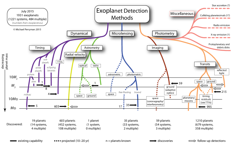
Figure 1: Graphics to indicate the number of exoplanet detections using a particular detection method. Courtesy: M. Perryman

The prevalence of solid material suggests that the main formation process has started from the accumulation of small bodies via sequential accretion where bodies grow through a sequence of trillions of collisions from small dust particles to full fledged planet. Additionally, the flat structure of the Solar System indicates that this process has taken place within a protoplanetary disk, the Solar Nebula, that orbited the early Sun. These findings are supported by the observational fact that many protostars are surrounded by a flat disk consisting of gas and dust, with extensions similar to that of the Solar System. This nebular hypothesis of the Solar System’s origin was already the basis of the formation theories of Kant and Laplace. While Kant focused on the evolution of the solid dust material in the Solar System 1755anth.book.....K , Laplace focused more on the hydrodynamical aspects 1776Laplace . Much later, V. Weizsäcker has taken up these ideas to develop his hydrodynamical theory of planet formation in a disk containing several vortices 1943ZA.....22..319W . An overview of these and many subsequent ideas are contained in 2000oess.book.....W or 1998Fahr . A modern (pre-extrasolar planet) review of the formation of the Solar System from an astrophysicists perspective is given by 1993ARA&A..31..129L , while the chronological aspect is emphasized by 2006EM&P...98...39M .

1.2 Properties of the extrasolar planets

During the past 20 years numerous extrasolar planets orbiting Sun-like stars have been detected, and their physical and dynamical properties provide us with the opportunity to examine the generality of our ideas about the planet formation process, and modify those chapters of the whole story that are not compliant with the new observational data. We will not go in any detail into the detection methods that are used to discover new planets, an overview is given in 2011exha.book.....P , and see also the lecture notes by A. Quirrenbach in the Saas-Fee Advanced Course 31 2006expl.conf....1Q . In Fig. 1 we display graphically the number of planets discovered using a particular detection method as of July, 2015. As shown, in absolute numbers the transit method has been by far the most successful method since over half of all detections have been achieved using transits, most of them with the Kepler space telescope. From the ground the radial velocity method is still the most successful. As shown, there are nearly 500 multiple systems. After the end of the regular Kepler-mission the rate of detections has somewhat slowed, but new space missions such as TESS 2015JATIS...1a4003R or PLATO 2014ExA....38..249R will surely enhance it again. A status of the actual numbers can be found in several online catalogues such as http://exoplanet.eu/, http://exoplanets.org, or http://www.openexoplanetcatalogue.com/.

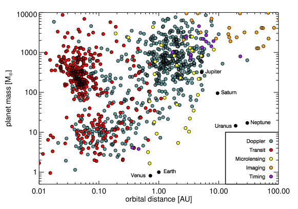
Figure 2: Mass of the extrasolar planets with respect to the distance from their host star. From Winn and Fabrycky 2015ARA&A..53..409W .

The amount of data collected so far allows for extensive statistical analyses of the exoplanet properties, which serves in particular to understand the similarities, as well as the differences with respect to our Solar System. A very important diagram is shown in Fig. 2 where we display the mass of the planet against semi-major axis. Unfortunately, for the Kepler planets their mass is known only for a small fraction of all discovered planets because the low apparent magnitude of the host stars does not allow for an easy radial velocity follow-up, but see 2014ApJS..210...20M , where this has been successful. Hence, the plotted data in Fig. 2 refer primarily to the radial velocity measurements. Here, one has to keep in mind that for this detection method the quoted masses refer to the minimum masses because of the unknown inclination to the systems. In the plot the different detection techniques have been indicated and it is clear that they are sensitive to different regions in the $M-a$ diagramme, but we will not discuss here any detection limits or biases. The planets populate different regions in the plot which have been used to separate the whole planet population into various planetary species. The top left corner, for semi-major axis smaller below about 0.1 AU and masses above 100 $M_{\oplus}$, is inhabited by the so-called Hot Jupiters, as these planets are comparable in mass to Jupiter in the Solar System but are located very close to the star such that the stellar irradiation leads to surface temperatures often well above 1000 K. Already the very first exoplanet discovered, 51 Peg 1995Natur.378..355M , with a 4 day period and a separation from the Sun about 1/20 AU, belongs to this category. It is very difficult to form such a planet at that location because the high disk temperatures do not allow for simple condensation of material. Hence, already this first discovery of an exoplanet required a modification to the standard planet formation theory by allowing some migration process 1996Natur.380..606L . Within the same mass range, or even a bit higher, up to 10 $M_{\rm Jup}$, and with a larger distance between 1 and 10 AU we find the classical giant planets, i.e. planets of Jupiter mass or higher within a similar distance from the star. Below these, there is a whole group of planets with masses between 2 and about 30 $M_{\oplus}$, and distances from 0.03 up to about 1 AU. These are the so-called Super Earths, as they are located in the same distance regime as our home planet but with a somewhat larger mass. Even though not directly apparent in this limited sample plot, from the Kepler data it is clear that the smaller planets are by far the largest population of the detected exoplanets. Only less than 10% of all Kepler planets are larger than Jupiter while nearly half are in the range of Neptune, with (2 – 6) $R_{\oplus}$, and the rest smaller (for the most up to date statistics on the distribution of planetary radii of Kepler-planets we refer to the NASA-Homepage). Observational limitations do presently not allow for the detection of the very low mass and small objects in this regime, but from statistical analyses it is estimated that at least 11% of Sun-like stars harbor an Earth-size planet receiving between one and four times the stellar intensity as Earth 2013PNAS..11019273P , a statement with strong implication with respect to the possibility of life in the Milkyway.

Concerning the shape of the orbits it became clear very early on that the average eccentricity of exoplanets is with $\bar{e}\sim 0.3$ much higher than for the Solar System. This value applies for the radial velocity planets, which show a weak trend of an increase in $e$ for larger planet masses. The Kepler systems show, on average, a smaller eccentricity and have lower planet masses. The main orbital and dynamical properties of exoplanets have recently been summarized in 2015ARA&A..53..409W . From a formation point of view it is noteworthy that the multi-planet systems show only a very small mutual inclinations between the planetary orbits, i.e. planetary systems are born flat. Interestingly, this applies to the circumbinary planets as well which indicates that the protoplanetary disks from which the planets formed were closely aligned with the central binary star.

1.3 Pathways to planets

After having summarized briefly the observational aspects of planetary systems including our own, we will in the following sections outline the process of formation, based on the modern day view. Historically, the Greek philosophers have already theorized a long time ago about the origin of the Earth and possible other Worlds. In the 5th century BCE Leukippos suggested that the worlds form in such a way, that the bodies sink into the empty space and connect to each other, as translated in 1998gdav.book.....H . In a very broad sense this is still the view today, because with World the whole Solar System is implied, Sun and all planets. As we know today, stars form within a collapsing molecular cloud that turns into a highly flatted configuration due to angular momentum conservation. In the center the proto-sun forms and in the disk the planets. The problem we are facing is, that we need to illuminate a process that for the Solar System took place 4.5 billion years ago. Nevertheless, the observational data from the Solar System, the data from protoplanetary disks and last not least the large and growing sample of extrasolar planetary systems allow us to draw a coherent framework in which many details are left to be worked out but the main processes have probably been understood.

Two main pathways to make planets have been discussed in the literature. In the first scenario, planets are believed to have formed directly from the protoplanetary disk by gravitational instability. In this top-down process spiral arms become gravitationally unstable and fragment directly to form large protoplanets. The advantage of such a process may be the possibly very fast formation timescale ($\sim 1000$ years) but for typical protoplanetary disks the required fast cooling of the disk material is probably not satisfied expect possibly for very large distances (several 10s of AU) from the star. In addition, the Solar System contains a multitude of small solid objects and the giant planets have most likely massive solid cores in their centers. These problems of the GI-scenario, and the properties of the Solar System have led to the current view that the planet formation has occurred predominantly via a bottom-up process in which small dust particles have grown through millions and millions of sticking collisions to form eventually large protoplanets, terrestrial planets, and the cores of the giant planets. The giants collect by their strong gravitational force in a final step a large amount gas.

Hence, in the following we describe the planet formation process on the basis of the sequential accretion scenario, where we start out in Sect. 2 with the growth from small dust to km-sized planetesimals, study the formation of terrestrial planets in Sect. 3. The growth to massive planets via core-accretion will be described in Sect. 4 followed a description of the GI pathway in Sect. 5. An important part of the planet formation process is the occurrence of dynamical evolution due to disk-planet interaction. We will describe the most important results in Sect. 6 of this lecture followed by a study of the dynamical behaviour of multi-object planetary systems in Sect. 7.

The physical and dynamical properties of the Solar System indicate that the planets formed in a flat disk orbiting the young proto-sun. The information drawn from the solid bodies implies that the growth occurred via a bottom-up process where planets were formed in a sequential accretion process starting from tiny interstellar dust grains, all the way to full grown planets. The additional information drawn from the large sample of extrasolar planetary systems supports this basic scenario but requires to take into account dynamical effects in multi-planet systems and the gravitational interaction between the disk and the growing planets.

2 From Dust to Planetesimals

Protoplanetary disks typically consist of a mixture of about 99% gas and a small amount ($\sim 1\%$) of solid, dust particles 2011ARA&A..49...67W . As mentioned above in the introduction, in the Solar System and many of the observed extrasolar planetary systems, the formation of planets is believed to be accomplished primarily through a sequential growth process starting from small interstellar dust particles. Hence, to study this early planet formation phase we need two ingredients, an initial ensemble of dust particles and a suitable disk model.

Concerning the dust, the now classical measurements of interstellar extinction 1977ApJ...217..425M have shown that interstellar dust grains have a size range of about $0.1-1.0\mu$m with a size distribution of $n(a)\propto a^{-3.5}$, where $n(a)$ denotes the number of particles with a given size $a$. New results indicate some deviation from this MRN-profile (after Mathis, Rumpl and Nordsieck, 1977ApJ...217..425M ), but the typical expected initial sizes of interstellar dust particles is probably within the indicated size range 2003ARA&A..41..241D . Through a sequence of trillions and trillions of collisions, starting from these tiny dust grains full grown planets are eventually assembled. In this section we deal with the first phase of this process and consider the initial growth up to about km-sized planetesimals.

Concerning the disk structure, one often refers to simple disk models where the density and temperature distribution can be described by suitable power laws, in order to simplify the analyses. Starting from the observed locations and masses of the planets in the Solar System, Hayashi & Weidenschilling 1981PThPS..70...35H ; 1977Ap&SS..51..153W constructed a simple relation for the variation of the surface density of the material with distance from the Sun. To this purpose they spread out the observed mass of the planets in a number of radial bins and added the amount of gas to match the observed dust/gas ratio in observed protoplanetary disk, typically 1/100 2011ARA&A..49...67W . This mass distribution is now referred to as the Minimum Mass Solar Nebula (MMSN) as it contains just the right total amount of matter and density slope to make the Solar System, as we observe it today. The resulting gas density distribution is then given by 1981PThPS..70...35H

$$\Sigma_{\rm g}(r)\approx 1700\,\left(\frac{r}{1\mathrm{AU}}\right)^{-3/2}\,\mbox{g/cm}^{2}\,.$$ (1)

Such a model yields a typical total disk mass of about $0.01-0.05$ M_⊙. Of course, initially the mass could have been substantially larger and the density distribution different, because planets tend to move (migrate) in disks and do not remain at their birth locations. Consequently, the simple distribution (1) has been criticized frequently and different slopes have been suggested 2007ApJ...659..705A ; 2007ApJ...671..878D , but is nevertheless still frequently used, let it be only as a suitable reference model. Observed disks typically tend to have a flatter profile and show at some radius a cutoff, as seen also in time-dependent viscous disks model 1974MNRAS.168..603L . Such distributions can be described in parameterized form as an exponentially tapered power law

$$\Sigma(r)\propto\left(\frac{r}{R_{\rm c}}\right)^{-\gamma}\,\exp\left[-\left(\frac{r}{R_{\rm c}}\right)^{2-\gamma}\right]\,.$$ (2)

Here the exponent $\gamma$ and the characteristic radius, $R_{\rm c}$, can be chosen to match the observations. For $\gamma$ mean values of about 0.9 have been determined while the value of $R_{\rm c}$ ranges from $20-200$ AU 2011ARA&A..49...67W . For the temperature in the disk one can assume as a first approximation a passive disk, where internal heat is solely generated by the illumination of the central star. At larger radii (beyond a few AU) this is a good approximation because there the internally generated heat is lower than stellar irradiation. In this case the radial temperature of the disk is given by 1981PThPS..70...35H

$$T(r)\approx 280\,\left(\frac{r}{1\mathrm{AU}}\right)^{-1/2}\,\mbox{K}\,.$$ (3)

This distribution assumes a vertically isothermal stratification, hence eq. (3) describes the midplane as well as the surface temperature of the disk. Assuming now a constant temperature in the $z$-direction, the vertical hydrostatic equation can be solved for the density, and a Gaussian distribution is obtained, with

$$\rho(r,z)=\rho_{0}(r)\,\exp{(-z^{2}/H^{2})}\,.$$ (4)

Here $\rho_{0}(r)$ is the midplane density, $H(r)=c_{\rm s}/\Omega_{\rm K}$ the vertical scale height (often termed the disk half-thickness), $\Omega_{\rm K}(r)$ is the Keplerian rotational velocity in the disk, and $c_{\rm s}(r)$ the local sound speed. By integrating $\rho(r,z)$ over $z$ one obtains the radial surface density distribution

$$\Sigma(r)=\int_{-\infty}^{\infty}\rho(r,z)dz\,.$$ (5)

By varying the exponent $\gamma$ in eq. (2) different disk models can be constructed, that can be used as a basis for analyzing the dust motion within the disk. More detailed analytical disk models including internal as well as external heating have been calculated by 1997ApJ...490..368C .

These disk models can be used as a basis to study the motion and growth of embedded dust particles. As shown in the accompanying chapter by P. Armitage in this volume the particles have a different velocity as the gas because they do not feel the effects of gas pressure. As a consequence they experience a drag force which is proportional to the velocity difference between the gas and dust particles and depends on the size of the particle and the gas density. This frictional force leads to a drift of the particles which is directed towards the pressure maximum of the gas. As can easily be inferred from the gas and temperature distribution the pressure, that is $\sim\rho T$, drops rapidly with radius in a protoplanetary nebula. Consequently, the particles experience a rapid inward radial drift which is for typical disk parameter about $v_{\rm drift}\sim 50$m/s. This leads to a rapid loss of particles into the central star, and any successful growth process has to be sufficiently fast to overcome this drift-barrier. For more details on the motion of particles in gas disks see 1977MNRAS.180...57W , or the review article by 2010EAS....41..187Y . The overall growth phase from dust to planetesimals has been reviewed more recently in 2010AREPS..38..493C or 2014prpl.conf..547J .

2.1 Study the initial growth phase

Starting from the initially $\mu$m sized solid particles that are embedded in the accretion disk the growth process can only proceed through a sequence of collisions where two partners hit each other and stick together due to some adhesive forces. The outcome of these mutual collisions and the important sticking probability depend on the friction coefficients, the compactification of the material (i.e. how much kinetic energy can be dissipated upon collisions) and the relative velocity of the components in the collision process.

The actual growth of small particles has been studied in the laboratory and via numerical simulations, where for the latter the experimental results have been used to calibrate the simulations. On the experimental side the most complete set of studies have been performed using spherical, mono-disperse SiO₂ particles (silica) that have the additional advantage of an easy direct usage in numerical studies 2008ARA&A..46...21B . Although these particles seem to be rather special, experiments have indicated that the variations in material properties between silica and silicates (that are often detected in protoplanetary disks) do not seem to play a major role in comparison to morphological and size differences 2000ApJ...533..454P . Hence, the usage of this material in the laboratory studies seems to be well justified. In the following we describe the basic results of the laboratory work and the numerical studies.

Experiments

The experimental studies have been performed under a variety of different laboratory setups, partly under vacuum and zero gravity conditions. For the latter the following facilities have been utilized: the fall-tower in Bremen, parabola flights as offered for example by ESA, and the international space station. The outcome of these series of experimental studies have been summarized exhaustively in the review article 2008ARA&A..46...21B , and we will focus here on the main results.

For the very small $\mu$m sized particles the initial growth is very clearly fractal, i.e. the mass-size relation is given by

$$m\propto s^{D_{\rm f}}$$ (6)

with a fractal dimension $D_{\rm f}$ smaller than 3. Here $s$ denotes the size of the particle (effective radius) with mass $m$. The fractal growth can be understood by the fact that small particles are well coupled to the gas and do show only very small relative velocities with respect to each other. For the experiments relative velocities $v_{\rm rel}\approx 10^{-4}-10^{-2}$ m/s between the individual collision partners have been used. Hence, upon collisions the direct sticking of individual particles/aggregates dominates over restructuring effects, and the aggregates display a strongly elongated shape, with a fractal dimension typically such that $1.4\leq D_{\rm f}\leq 1.8$. Images of the fractal agglomerates and their mass growth in time are shown in 2000PhRvL..85.2426B ; 2004PhRvL..93b1103K .

The subsequent growth after the initial fractal phase has been studied through experiments using multiple collisions between the aggregates. In the experimental setup of 2009ApJ...696.2036W particles were enclosed in a plexiglass box whose floor could vibrate with a frequency of about 100 Hz. Using a high speed camera snapshots of the aggregates were taken and their mutual velocities and changes in mass/volume during collisions were measured. The observed typical collision velocities for the particles have been in the range of $0.1-0.3$m/s. An important quantity to describe the compactness of an agglomerate is the filling factor $\phi$ that gives the mass (density) ratio of a porous aggregate to a solid object of the same base material and same volume (i.e. $\phi$ is also referred to as the volume fraction of the material)

$$\phi=\rho_{\rm agg}/\rho_{\rm mat}\,.$$ (7)

Initially, the prepared ’dust-cakes’ are extremely fluffy and have a small filling factor of $\phi\approx 15\%$ which refers to a mean density of only $\rho_{\rm agg}=0.3$g/cm³ given that the solid matter density of SiO₂ is about $2.0$g/cm³. Often the porosity is quoted which is in a sense complementary to $\phi$ and given by $1-\phi$. The main outcome of these experiments (using mm sized particles) is a restructuring and compactification of the aggregates such that the fractal dimension $D_{\rm f}$ is increasing 2009ApJ...696.2036W . In terms of filling factor, starting from $\phi_{0}=0.15$ it increases with the number of collisions, $n$, according to

$$\phi(n)=\phi_{\rm max}-\Delta\phi\cdot e^{-n/\nu}\,,$$ (8)

where $\phi_{\rm max}$ is the final value of the filling factor, $\Delta\phi=\phi_{\rm max}-\phi_{0}$, and $\nu$ a constant determined to about $700$. The final filling factor reached is about $\phi_{\rm max}=0.365$. This compaction of the aggregates changes the surface to mass ratio, which is crucial for the dynamical behaviour of the particles in the protosolar nebula 1993prpl.conf.1031W . At the same time this restructuring modifies the macroscopic material parameter that determine the tensile, shear and compressive strength of the material (see below), which is turn alters their behaviour in subsequent collisions.

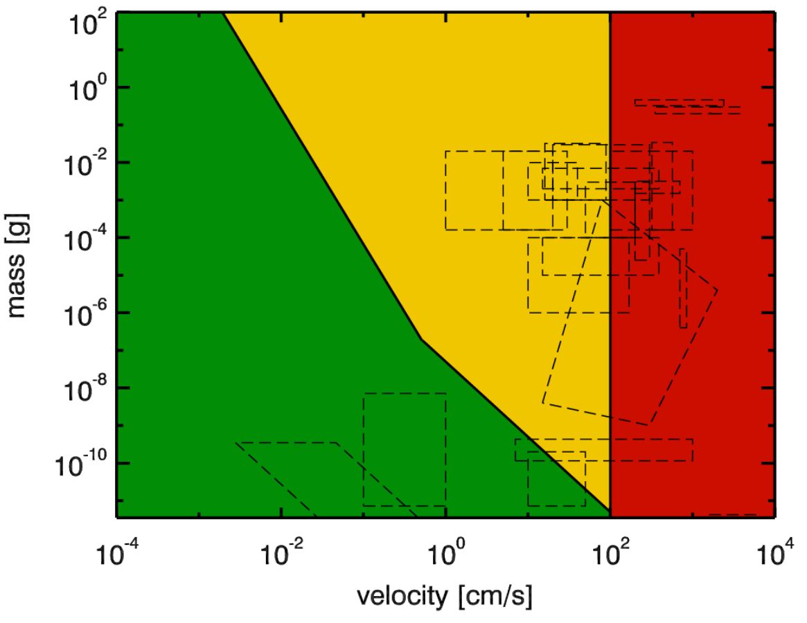
Figure 3: The results of laboratory experiments with respect to the outcome of mutual collisions of equal sized dust aggregates. Green areas indicate sticking collisions, yellow bouncing ones, and red corresponds to fragmentation of the aggregates. The collision experiments correspond to the areas within the dashed lines. Courtesy: Jürgen Blum

In addition to the described results, a multitude of additional collision experiments have been performed and analyzed, see e.g. 2008ARA&A..46...21B for an overview. In 2010A&A...513A..56G the physical outcomes are classified with respect to different collision channels corresponding to sticking, bouncing, fragmentation, or mass transfer from one aggregate to the other, see also 2011A&A...531A.166G for an alternative classification scheme. A summary of the experimental results is presented in Fig. 3 where on the $y$-axis the mass of collision partners is plotted and on the $x$-axis the relative collision velocity. In all analyzed collisions the two colliding objects have the same size. The areas enclosed by the dashed lines have been covered by the experiments of the research groups in Braunschweig (around Jürgen Blum) and Duisburg (around Gerhard Wurm). The colored regions indicate different growth or destruction regimes. In the green area the two aggregates stick together (growth regime), in the yellow one they bounce off each other (neutral regime), and in the red areas they are shattered into pieces and fragment (destruction regime). For net growth, one clearly has to be in the green regime, i.e. sufficiently small relative velocities. The diagram makes it very clear that there are different obstacles to the successful growth from small sized grains to planetesimals, these are basically the bouncing barrier 2010A&A...513A..57Z (the transition from green to yellow) and the fragmentation barrier (the transition from yellow to red). Obviously, above $v_{\rm rel}\approx 1$m/s growth is extremely difficult to achieve. Together with the drift barrier, mentioned above, these obstacles to successful growth are sometimes referred to as the meter-sized barrier to planetesimal growth 2008ARA&A..46...21B , as it is difficult to achieve growth beyond 1 m in size. We will comment on possible pathways to overcome these obstacles to further growth in Sect. 2.2 below.

Numerical studies

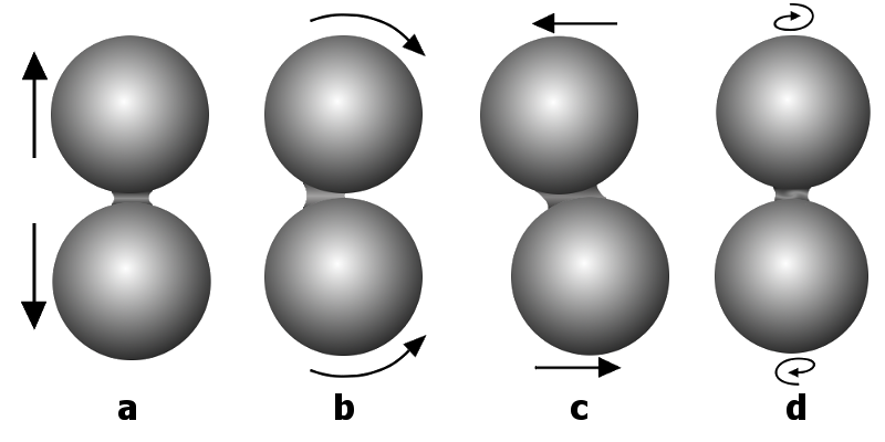
Figure 4: Schematic view of the different type of interactions between two individual spherical monomers. These correspond to a) Compression/Adhesion, b) Rolling, c) Sliding, and d) Twisting. Courtesy: Alexander Seizinger

A very useful alternative to real laboratory experiments is performing numerical experiments and study collisions in the computer using appropriate models to simulate reality. In the case of planetesimal growth two approaches have proven to be useful. In the first approach the behaviour of aggregate collisions is simulated on a microscopic level using a direct molecular dynamics (MD) approach with suitable forces between the individual $\mu m$-sized monomers that the whole aggregate is composed off. In a second approach, suitable for larger particles, a continuum model is constructed using averaged material parameters (such a elasticity, strengths, sound speed, etc.). We will discuss both approaches in this section.

The MD approach relies on modeling in detail the microscopic interaction between two individual monomers, using nanoscale molecular forces, such as the van der Waals force or other electrostatic forces. In the case of dust aggregates the forces can be divided into 4 categories as depicted in Fig. 4, see 2007ApJ...661..320W and references therein. The formulation of the forces is based on a microscopic approach, and the implementation and application to the physics of dust coagulation under astrophysical conditions has been described in 1997ApJ...480..647D . For the standard normal relative motions between individual monomers (panel $\bf a$ in Fig. 4) the force is based on the JKR-theory (after Johnson, Kendall and Roberts, 1971RSPSA.324..301J ), that constitutes an improvement to the original model which is due to to Heinrich Hertz 1882Hertz . The rolling ($\bf b$), sliding ($\bf c$) and twisting ($\bf d$) frictional forces have been calculated by Dominik & Tielens, for example in 1995PMagA..72..783D , see summary in 1997ApJ...480..647D . As hinted in Fig. 4 by the ’necks’ between the two spheres, the intermolecular forces show a hysteretic behaviour. The forces between two monomers do not only depend on the actual distance but on the past history. The forces between approaching particles, that have not been in contact yet, is different from the force (at the same separation) if they just had been in contact. The way to imagine this is to assume that the particles are surrounded by a thin layer of honey or glue. Before coming into contact there is no attractive fore, but after separation a neck is formed that pulls the particles back together. The physical model by Dominik & Tielens does take account for these hysteretic, dissipative effects.

Later the model was improved by deriving the forces (torques) from appropriate potentials which allows for detailed tracking of the different energy channels during the collisions 2007ApJ...661..320W . Before applying the numerical model to physical collisions several numerical parameter have to be adjusted properly. This is done by comparing the results of numerical simulations directly with laboratory experiments. In these well constructed experiments a small dust aggregate (dust-cake) is prepared by simple ballistic aggregation procedure which leads to a sample with an initial filling factor, $\phi=0.15$. The dust-cake is then contained between two walls and compressed from above 2009ApJ...701..130G . Upon the compression the filling factor $\phi$ increases and the pressure on the adjacent walls as well. The important quantity to calibrate is the pressure-porosity relation, that shows a characteristic behaviour, which depends on the geometry of the particular setup. Calibrations of this type have been done by 2008A&A...484..859P and later by 2012A&A...541A..59S who found for example a modification of the rolling and sliding coefficients.

After a successful calibration process the numerical simulations allow to determine continuum properties of the aggregate, such as sound speed or the shear modulus. These are sometimes difficult or impossible to determine experimentally. In numerical simulations special treatments, such as adding a sort of glue between the particles and the wall can be introduced to make these measurements numerically possible. Having successfully determined these parameter a new type of simulations can be performed where the aggregates are treated as a smooth continuum average over the local details. In the astrophysical community a very important, successful and widespread method is Smooth Particle Hydrodynamics (SPH). Here, the continuum is modeled again by individual ’particles’ but now they do not represent individual monomers or real physical particles but they can rather be considered as a sort of Lagrangian nodes that move in space and time. Quantities such as density or pressure are obtained from a suitable averaging procedure over neighboring particles. The method was initially developed for simulating purely hydrodynamic flow (see review by Monaghan 2005RPPh...68.1703M ) but was later extended to model the dynamics of solid objects, where time dependent equations to follow the stresses within the body are added and solved simultaneously. In addition, the method has been augmented by an elasto-plastic model, and special treatments for handling cracks and fragmentation have been implemented 1994Icar..107...98B . Hence, these type of simulations allow to model the collisions of larger objects, starting from dm-size up to very large objects where internal gravity may play a role. Indeed, using the SPH method collisions between objects that range in size from m-sized bodies up to the Moon forming impact between the proto-Earth and a Mars-sized object have been simulated 1999Icar..142....5B ; 1986Icar...66..515B .

Similar to the collisions between tiny particles those between macroscopic objects will lead to a fragmentation and destruction of the (larger) target if the relative collision speed becomes too large. To analyse the outcome of these object-object ’encounters’ the specific collision energy between target and projectile is a useful quantity. It is defined as

$$Q_{\rm D}=\frac{1}{2}\frac{m_{\rm proj}v^{2}_{\rm rel}}{M_{\rm target}+m_{\rm proj}}\,,$$ (9)

where $m_{\rm proj}$ is the mass of the projectile, $M_{\rm target}$ the mass of the target and $v_{\rm rel}$ the relative velocity between the two objects.

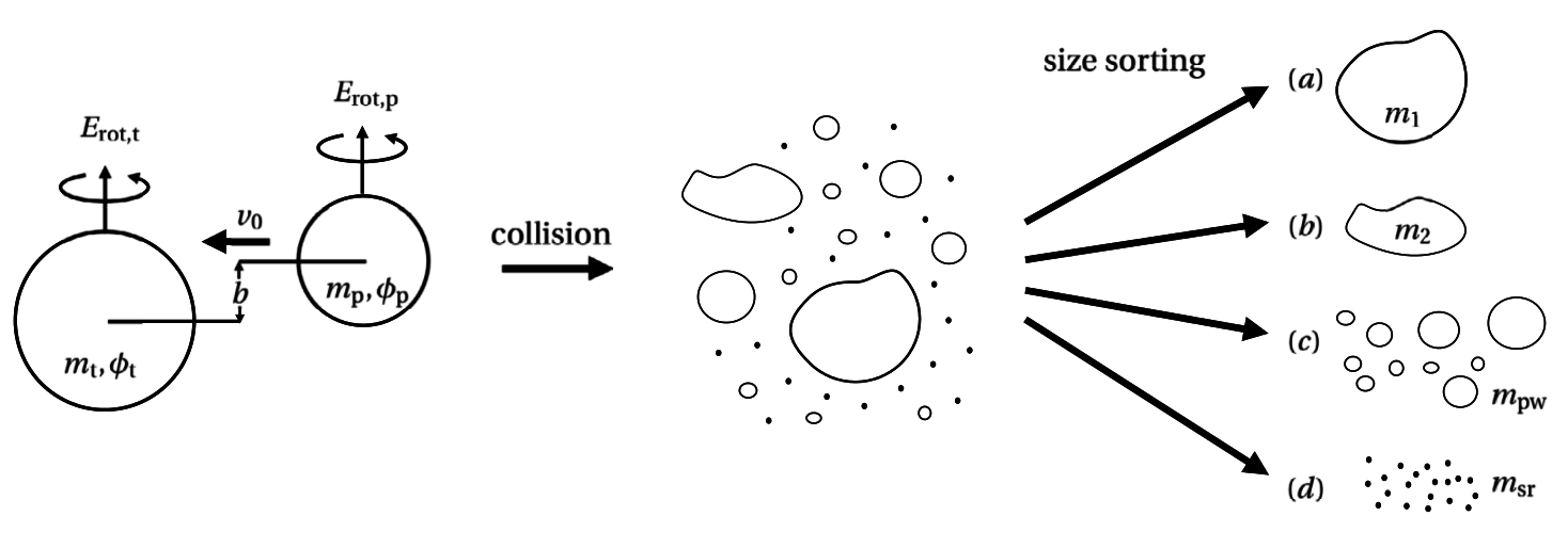
Figure 5: Schematic representation of the outcome of a collision between two objects. The left side displays the situation before the collision: the target (t) and projectile (p) collide with impact velocity $v_{0}$, and impact parameter $b$. Before the collision they are described by their mass ($m$), filling factor ($\phi$) and rotational energy ($E_{\rm rot}$). The outcome consists of different groups: a) the largest fragment; b) the second largest fragment; c) the power law population; and d) the sub-resolution population. This classification scheme is based on the four-population model by 2011A&A...531A.166G .

The general outcome of collisions is well described in Fig. 5. It consists typically of a limited number of bigger objects (here cases $\bf a,b$ on the right hand side), a large number of smaller particles ($\bf c$) that follow approximately a power law size distribution 2009Icar..199..542l , and a ’sea’ of very small particles ($\bf d$) that are too small to be resolved (at least numerically). The four-population model of 2011A&A...531A.166G assumes that there are only two major objects after the collision. The catastrophic destruction threshold, $Q^{*}_{\rm D}$, is now defined as that specific collision energy at which the largest remaining fragment has 1/2 of the target mass. As a function of target size $Q^{*}_{\rm D}$ has a $V$-shaped behaviour, in the strength dominated regime (for target radii smaller than about 1 km) $Q^{*}_{\rm D}$ is decreasing with increasing target size. For larger objects gravitational re-accumulation becomes important and the mass of the largest post-collision object increases, hence $Q^{*}_{\rm D}$ increases again with target size in this gravity dominated regime. The minimum occurs at the transition between the two regimes. Using the SPH-method numerical experiments of collisions between two basalt spheres with radii between 100m to 10km using different relative velocities have been performed 1999Icar..142....5B . The results show that for a typical velocity, $v_{\rm rel}=20$km/s, the weakest bodies (with minimum $Q^{*}_{\rm D}$) are those with radii of about 300m, here $Q^{*}_{\rm D}$ has values of about $10^{2}$[J/kg]. Later 2009Icar..199..542l constructed fit formulae to calculate $Q^{*}_{\rm D}$ as a function of target radii which can be used in statistical simulations for an ensemble of objects (e.g. asteroids or Kuiper belt objects) to follow their time evolution 2013AJ....146...36S .

2.2 How to overcome growth barriers

As sketched out for example in Fig. 3, from laboratory experiments it is known that the mutual collisions of mm to cm-sized aggregates result frequently in bouncing, e.g. 2009ApJ...696.2036W ; 2010Icar..206..424H ; 2012Icar..218..688W ; 2012A&A...542A..80J . Incorporating the data from the various experimental setups, 2010A&A...513A..56G constructed an algorithm to to describe analytically the results of mutual collisions of aggregates as a function of their relative collision speed, their mass and their porosity. This model was then used to simulate the evolution of a swarm of dust aggregates in a protoplanetary disk in a statistical manner 2010A&A...513A..57Z . Initially the aggregates grow by the above described process, but for larger sizes the relative velocities increase. Due to the higher kinetic impact energy the aggregates become more and more compacted during successive collisions. If the aggregates get too compact, i.e. the filling factor reaches values up to about $\phi\sim 0.4$, then mutual collisions do not result in sticking anymore, rather they bounce off each other and the growth process is terminated 2010A&A...513A..56G . In agreement with the experiments this occurs within a size regime of centimeters to decimeters, and was termed the bouncing barrier 2010A&A...513A..57Z .

In early numerical studies to understand the origin of the bouncing it was found that for the aggregate parameters used in the experiments typically sticking occurs, and bouncing only for much larger filling factors above $\phi=0.5$ 2009ApJ...702.1490W . In subsequent numerical simulations the condition for rebound (bouncing) has been studied in more detail by Wada et al. 2011ApJ...737...36W who showed that it depends on the coordination number, $n_{\rm c}$, of the individual monomers, which describes the number of contact points (neighbors) an individual monomer has. Clearly, the more contacts an aggregate has the stiffer it reacts to collisions promoting bouncing rather than sticking, and a value of $n_{\rm c}=0.6$ above which bouncing occurs has been found in the simulations 2011ApJ...737...36W . Obviously, the higher the filling factor the larger the coordination number has to be. However, as shown recently there is not a one-to-one relation between $\phi$ and $n_{\rm c}$ 2013A&A...551A..65S . The number of contacts that a specific aggregate with a given porosity has, depends on the process by which it has been constructed. In laboratory experiments using aggregates composed of micron-sized dust grains, it is usually only possible to determine the global filling factor (via the mean density) but not the local coordination number which is a microscopic quantity. Thus, one has to be very careful when comparing results from numerical simulations for a given filling factor directly to results from laboratory experiments that use the same $\phi$.

Even though the numerical studies are still not in full agreement with the experiments in the bouncing regime, there are indications that non head-on collisions lead to increased bouncing 2013A&A...551A..65S . Additionally, it was shown that for larger aggregate sizes the fragmentation velocity becomes higher, about 10 m/s. Despite these purely geometric characteristics of the collision the sticking probability could be enhanced by special material properties, such as sticky organic materials, magnetic or charged particles. However, as discussed in 2008ARA&A..46...21B the effects probably do not change the growth efficiency significantly. Another option is the aerodynamic re-accretion as suggested by 2001Icar..151..318W . Here, the idea is that after a nearly destructive collision the small fragments that surround the largest fragment fall back it due to aerodynamic drag exerted on them. By this mechanism it is possible that the majority of particles become re-accreted leading to a net growth. The process depends on the properties of the growing body in particular its porosity with respect to the gas flow through it and on the speed of the ejecta, and its importance for a successful growth is not fully settled 2008ARA&A..46...21B .

In a process related to aerodynamic re-accretion the bouncing barrier can be overcome by a sweep-up process. Using the standard results from the collision experiments in a coagulation code one finds for the general dust population that bouncing collisions prevent any growth above millimeter-sizes. However, adding in the models a few cm-sized particles to a sea of smaller ones, which could happen in a real disk for example by vertical mixing or radial drift, these can act as a catalyst by starting to sweep up the smaller particles, which results in very rapid growth. As shown in 2012A&A...540A..73W using this mechanism, 100-m-sized bodies can be formed on a timescale of 1 Myr at a distance of 3 AU from the central star. In this process the existence of the bouncing barrier is highly beneficial for promoting growth, as it prevents the formation of too many larger particles that would otherwise destroy each other via fragmenting collisions. Hence, a reservoir of small particles is maintained that can be swept up by larger bodies. The single requirement for this greatly enhanced growth process is the creation of a few lucky particles of cm-size or larger that can then sweep-up the smaller ones 2012A&A...540A..73W .

A possibility to overcome the fragmentation barrier is through collisions of particle with very different sizes. As shown in some experimental studies 2005Icar..178..253W , collisions between millimeter-sized dust projectiles and centimeter-sized dust targets lead to net mass growth of the target up to collision velocities of 25 m/s. The authors suggest that for even higher velocities growth can be achieved which supports the idea that planetesimal formation via collisional growth is a viable mechanism at higher impact velocities. Following up on this this idea of high velocities and different collision partners, 2012A&A...544L..16W and 2013ApJ...764..146G demonstrated that it is the combination of a statistical relative velocity distribution function in the coagulation models and high-mass-ratio collisions that allows for successful growth of larger bodies. The velocity distribution allows to overcome the bouncing barrier, and the different masses to cross the fragmentation barrier 2005Icar..178..253W . 2013ApJ...764..146G even suggest that via this mechanism the problem of planetesimal formation close to the central star, the presence of millimeter- to centimeter-sized particles far out in the disk, and the persistence of $\mu$-sized grains for millions of years, can be solved.

In the outer regions of the protoplanetary-disk the growth of particles is made easier by two effects. First, water has condensed to ice beyond the so-called snow line at temperatures below about 170 K, which increases the local surface density of solids by about a factor upto 4 1981PThPS..70...35H . In addition to the enhanced surface density of the solid particles the icy particles stick together up to much higher relative velocities of about 50 km/s 2011ApJ...737...36W . The higher density and improved stickiness clearly will enhance the growth of small bodies. For disk parameter according to the MMSN the snow line lies around 2.7 AU in good agreement with the location of the planets in the Solar System 1981PThPS..70...35H . In addition, the sudden change in the opacity of the disk at the snow line will lead to a reduction in turbulent activity in the disk and subsequently to a pressure maximum of the gas, which in turn will further increase the local surface density of solid particles because they drift towards the local pressure maxima 1977MNRAS.180...57W . Hence, the inward drift of particle is prevented at the snow line and the growth of planetesimals enhanced 2007ApJ...664L..55K . Finally, considering the low catastrophic destruction threshold of 10 m sized objects made of basalt, recent SPH simulations have indicated that the inclusion of a porous equation of state allow non-fragmenting collisions to higher velocities 2011A&A...531A.166G .

2.3 Dust concentration

As mentioned above there are several new suggestions available now how to overcome the growth barriers on the way from dust to planetesimals. The suggested mechanism rely on a better understanding of individual collisions and a statistical treatment of a whole ensemble of growing objects. Another, often discussed mechanism to cross the growth barriers is the pre-concentration of particles in inhomogeneities of the protoplanetary disk. Often discussed has been the collection of particles in turbulent eddies or in vortices. When the dust concentration has reached a critical value a streaming instability can set in 2005ApJ...620..459Y , and gravity can lead to rapid growth to larger objects 2007Natur.448.1022J . Similarly gravitational instability in the condensed dust layer in the midplane of the disk dust layer could enhance planetesimal growth 1973ApJ...183.1051G . These mechanisms have been presented in detail in the contribution by P. Armitage and will not be discussed here further.

The initial growth from dust to planetesimals suffers a growth crisis when particles reach a typical size of about decimeter to meter. In this regime, the particles experience the fastest radial drift and possible loss into the star and collisions often lead either to destruction or bouncing and no net growth. While this obstacle is presently not fully mastered, several possible new paths have been investigated recently to solve the problem. These include a better understanding of individual collisions, improvements in the statistical treatment as well as large scale collective effects by interaction with the ambient disk.

3 Terrestrial planet formation

In this chapter we describe the growth from planetesimals to full terrestrial type planets. Following 2006expl.conf..369C we define a planetesimal to be an object large enough that the motion of nearby particles are significantly perturbed through gravitational interaction. This implies that the velocity perturbations induced by planetesimals are larger than the typical drift velocity of particles which is about $10$ m/s. Hence, the term planetesimal refers then to objects of a km in size or larger, while below this size the term pre-planetesimal is sometimes used 2011A&A...531A.166G . As we shall see, this growth from km-sized planetesimals to a full grown terrestrial planet several 1000 km in size proceeds in two major steps that are quite different in duration. In the first phase the planetesimals grow in a fast, runaway process to produce a relatively small number of Moon to Mars sized planetary embryos (also called protoplanets). After this phase, the inner parts of the protoplanetary disk contains very little amounts of gas and the embryos grow via a much longer collisional phase to a set of terrestrial type planets. Excellent overviews on this era in the history of the planet formation process have been presented elsewhere 2004E&PSL.223..241C ; 2012AREPS..40..251M .

3.1 Concepts

Before going into the actual growth scenario from planetesimals to protoplanets we explain a few important physical concepts or processes that are of relevance with respect to this phase in the planet formation process. The problem we are facing when growing in size from few km-sized planetesimals to Moon-sized planetary embryos, is the fact that for this mass range the aerodynamic drag forces become negligible and cannot serve anymore to provide for any change in the relative velocity between particles necessary to have collisions. Additionally, the induced inhomogeneities in the disk by the growing object are not strong enough yet to provide significant drag and subsequent migration. Finally, with initial 1 km-sized planetesimals over $10^{11}$ particles are required to make an embryo. This is numerically very demanding as it requires lots of particles and very long evolution times (a few 10 million years), see 2006expl.conf..369C . Consequently, this part of planetary growth is described best by a combination of statistical and numerical methods.

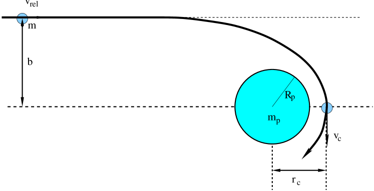
Figure 6: Principle of the gravitational focusing process. A small body with mass $m$ approaches a larger planetesimal with mass $m_{\rm p}$ with impact parameter $b$ and relative velocity $v_{\rm rel}$. Gravitational attraction results in a close encounter with smallest distance $r_{\rm c}$, and velocity $v_{\rm c}$ at the time of closest approach.

Gravitational focusing

The solid bodies can only growth via physical collisions, i.e. the shortest approach of two objects must be smaller than the sum of their radii. Here, we assume that the growing planetesimal has a radius $R_{\rm p}$ and that the accreted particle with radius $R$ is much smaller than this, $R\ll R_{\rm p}$. The geometrical cross section for such a collision is then given simply by $\sigma_{0}=\pi R_{\rm p}^{2}$. If there were no other means of increasing $\sigma_{0}$ then planetary growth would finish soon. Fortunately, when the objects become a few km in size the situation becomes much more favorable because the gravitational interaction between the two bodies will start to play an important role in bringing the particles closer together, a process called gravitational focusing. Let us consider the situation of two objects that have masses $m_{\rm p}$ (the large body) and $m$ (the small body to be accreted) which have initially the relative velocity $v_{\rm rel}$ with the impact parameter $b$, as shown in Fig. 6. To have a physical collision between the two objects the distance of closest approach, $r_{\rm c}$, must be smaller than $R_{\rm p}$, i.e. $r_{\rm c}<R_{\rm p}$. As the sketch in Fig. 6 implies the number of particles that possibly can directly hit the growing planetesimal is greatly enhanced over the purely geometrical cross section $\sigma_{0}$. The enhancement of the cross section through gravitational focusing can be obtained from the conservation of angular momentum and energy, by considering the initial state when the objects are very far away from each other and the situation of closest approach. We neglect the presence of the very distant central star and considering only these two objects. To have a physical collision we require that $r_{\rm c}=R_{\rm p}$, and angular momentum conservation yields

$$b\,v_{\rm rel}=R_{\rm p}\,v_{\rm c}\,,$$ (10)

where $v_{\rm c}$ is the velocity at the closest approach (Fig. 6). Energy conservation (in the center of mass frame) gives

$$\frac{1}{2}\mu\,v_{\rm rel}^{2}=\frac{1}{2}\mu\,v_{\rm c}^{2}-\frac{G(\mu M_{\rm tot})}{R_{\rm p}}\,,$$ (11)

with the reduced mass $\mu=mm_{\rm p}/(m+m_{\rm p})$ and total mass $M_{\rm tot}=m+m_{\rm p}$. Here we assumed that initially the two particles are sufficiently far apart such hat we can neglect the potential energy on the left side of eq. (11), and on the right-hand side we evaluated the energy again at the point of closest approach. Combining these two equations results in the following expression for the effective cross section, $\sigma$, of the interaction

$$\sigma\equiv\pi b^{2}\,=\,\pi R_{\rm p}^{2}\,F_{\rm grav}\,=\,\sigma_{0}\left[1+\left(\frac{v_{\rm esc}}{v_{\rm rel}}\right)^{2}\right]\,,$$ (12)

where we introduced the joint escape velocity

$$v_{\rm esc}=\left(\frac{2GM_{\rm tot}}{R_{\rm p}}\right)^{1/2}\,,$$ (13)

and the gravitative focussing factor over the purely geometrical cross section

$$F_{\rm grav}=\left[1+\left(\frac{v_{\rm esc}}{v_{\rm rel}}\right)^{2}\right]\,.$$ (14)

From eq. (12) and Fig. 6 we can see that for large relative velocities only particles that arrive directly from the front of the object will collide with it, i.e. the effective cross section is just the geometric one. On the other hand for small relative speed, i.e. in a cold disk of planetesimals with $v_{\rm rel}\ll v_{\rm esc}$, particles feel their mutual gravitational attraction for a longer time and hence particles from further away will be the drawn in. The effective cross section is then much higher than without gravity, i.e. $\sigma\gg\sigma_{0}$ or $F_{\rm grav}\gg 1$. The quantity $\theta=(v_{\rm esc}/v_{\rm rel})^{2}$ in eqs. (12) or (14) is sometimes called the Safronov number after an early pioneer in studying the formation of the Solar System 1972epcf.book.....S . If the approaching body is of size similar to the accreting planetesimal, then we can set $R_{\rm p}\rightarrow R_{\rm p}+R$ in the above formula for $v_{\rm esc}$.

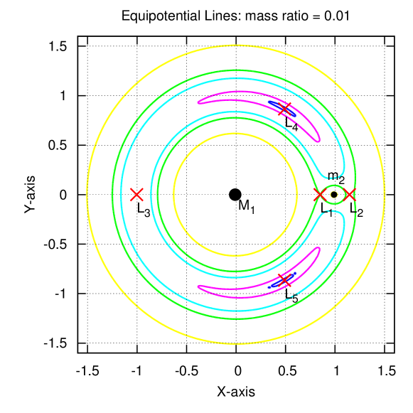
Figure 7: The dynamical structure of the restricted circular three-body problem. Shown are equipotential lines of the corotating potential (eq. 16) of a central star ($M_{1}$) which is orbited by secondary object ($m_{2}$). The classical 5 Lagrange points, $L_{1}$ to $L_{5}$ (marked by the red crosses), correspond to extrema of the potential.

The Hill-radius

Another important concept in this context is the definition of the Hill-radius. Here one considers the motion of a small (massless) particle in the presence of two larger gravitating bodies, that orbit each other on circular Keplerian motion. This is the so-called circular restricted three-body problem. In today’s Solar System the primary (largest) object is the Sun, the secondary for example Jupiter and the third massless particle a small asteroid. In our planet formation context the following objects are considered: a protostar with mass $M_{*}$, the growing planetesimal (mass $m_{\rm p}$) and a small particle (much smaller mass) to be accreted onto the planetesimal. As the motion of the star and the planetesimal is not affected by the small particle, these orbit each other with Keplerian motion, i.e. with an orbital speed

$$\Omega_{p}=\sqrt{\frac{G(M_{*}+m_{\rm p})}{a_{\rm p}^{3}}}\,\approx\,\sqrt{\frac{GM_{*}}{a_{\rm p}^{3}}}\,,$$ (15)

where $a_{\rm p}$ is the semi-major axis of the planetesimal.

The type of motion of a massless (low mass) particle in the presence the other two can be most easily derived from the effective gravitational potential written in a coordinate frame that rotates with the orbital speed, $\Omega_{p}$, of the growing planetesimal see 1999ssd..book.....M . In this corotating frame it reads

$$\Phi(\vec{r})=-\frac{GM_{*}}{|\vec{r}-\vec{r_{*}}|}-\frac{Gm_{p}}{|\vec{r}-\vec{r_{p}}|}-\frac{1}{2}\,\Omega_{p}^{2}\,r^{2}\,,$$ (16)

where $\vec{r_{*}}$ and $\vec{r_{p}}$ denote the positions of the star and planetesimal, respectively. The first two terms of the right hand side refer to the individual potentials of the star and planetesimal while the last term denotes the centrifugal potential as we consider the motion in the corotating frame. The equations of motion of the massless particle follow, as usual, from the gradient of the potential. As can be inferred from eq. (16) that shows selected equipotential lines for a secondary to primary mass ratio of $m_{1}/M_{*}=0.01$. The extrema of this potential are given as the roots of a 5th order polynomial, and one obtains the classical 5 Lagrange points, $L_{1}$ to $L_{5}$, as depicted in Fig. 7. The Lagrange points mark possible equilibrium positions of the particle but only two of those are stable, $L_{4}$ and $L_{5}$, which lie $60^{\circ}$ in front and behind the secondary. Typically one finds that the orbits are around the primary object, either inside the distance of the secondary (e.g. the main belt asteroids in the Solar System), or outside of it as indicated by the inner and outer lines in Fig. 7. For particles having the same semi-major axis as the secondary (here the planetesimal) the motion is either around one of the stable Lagrange points ($L_{4}$ or $L_{5}$) in so-called tadpole, or around both in horse shoe orbits 1999ssd..book.....M . The prime example from the Solar System are the Trojan asteroids that have the same semi-major axis and hence period as Jupiter and orbit around $L_{4}$ and/or $L_{5}$. For stability reasons these particles come never too close to the secondary object as can be seen by the equipotential lines in Fig. 16. If the object is in the very close vicinity of the secondary it is physically bound to it and orbits the secondary (e.g. the Galilean moons orbiting Jupiter). For our planetesimal this is the case for particle distances within a sphere of radius

$$R_{\rm H}=\left(\frac{m_{\rm p}}{3M_{*}}\right)^{1/3}\,a_{\rm p}\,$$ (17)

from the planetesimal. Here the index $p$ refers to the planetesimal. This sphere is enclosed between the Lagrange point $L_{1}$ and $L_{2}$ of the corotating potential, see Fig. 7. Using direct $3$-body simulations of a star, a planetesimal and small particles it was shown 1990Icar...87...40G that the motion of the particle to be accreted onto the planetesimal is highly chaotic in the vicinity of the planetesimal, in particular inside of the Hill-radius $R_{\rm H}$. These 3-body effects lead eventually to a limitation of the gravitational focusing factor $F_{\rm grav}$, that would otherwise diverge for small $v_{\rm ref}$, to maximum values of about $10^{4}$ 1993ARA&A..31..129L .

Modes of growth

The accretion of small particles leads to an increase in mass of the growing planetesimal. In general one can distinguish two modes of mass growth, ordered or runaway, as is schematically displayed in Fig. 8. In the ordered growth phase all objects grow at roughly the same rate and all the planetesimals in the whole ensemble have approximately the same size, hence this mode is sometimes called oligarchic growth 1998Icar..131..171K . On the other hand in the runaway case, one (or few) objects grow very rapidly at the expense of the smaller ones. What type of growth mode operates can be analysed for example by considering the relative growth of two particles with mass $m_{1}$ and $m_{2}$ which can be obtained by expanding the time derivative of the mass ratio

Figure 8: The two modes of mass growth. In the case of orderly growth the whole ensemble has always similar particle sizes, while in the case of runaway growth one particle grows rapidly in a swarm of smaller ones. (After E. Kokubo 2001RvMA...14..117K )

$$\frac{d}{dt}\left(\frac{m_{1}}{m_{2}}\right)=\frac{m_{1}}{m_{2}}\left(\frac{1}{m_{1}}\frac{dm_{1}}{dt}-\frac{1}{m_{2}}\frac{dm_{2}}{dt}\right)\,.$$ (18)

From eq. (18) we can infer that the relative mass growth, $1/m(dm/dt)$, for each object is important. Let us assume we start out with $m_{1}>m_{2}$, then we see that this ratio is increasing if the relative growth increases with $m$, because then the right-hand side in (18) is positive. This is exactly the situation for runaway-growth. On the other hand, if relative growth decreases with $m$ we have an ordered growth because then the mass ratio $m_{1}/m_{2}$ tends to unity. As we shall see in the following both growth modes occur during the assembly of protoplanets, the first growth is via a runaway process which is followed later by an orderly growth.

Using the cross section from eq. (12) we find for the mass growth of a planetesimal with mass $m_{\rm p}$

$$\frac{dm_{\rm p}}{dt}=\rho_{\rm part}\,v_{\rm rel}\,\sigma=\rho_{\rm part}\,v_{\rm rel}\,\pi R_{\rm p}^{2}\,F_{\rm grav}$$ (19)

where $\rho_{\rm part}$ is the density of the incoming particles. In deriving eq. (19) we have assumed that each collision will results in growth (100% sticking efficiency). The outcome of collisions of km-sized objects can obviously not be studied in the laboratory (where the maximum size is a fraction of a meter) and one has to rely on numerical simulations. Here, the results indicate that typically the collisions lead to net accretion 1999Icar..142....5B ; 2000Icar..146..133L unless the relative speeds are very high or the collisions are only grazing, but details depend on the internal strength of the colliding objects 2009ApJ...691L.133S .

Before we evaluate (19) for specific particle densities let us look at two illustrative examples (see 2010apf..book.....A ) that illustrate the different growth modes. Assuming a constant focusing factor, $F_{\rm grav}=const.$, we have for the mass growth of the planetesimal

$$\frac{1}{m_{\rm p}}\,\frac{dm_{\rm p}}{dt}\propto m_{\rm p}^{-1/3}\,.$$ (20)

For objects with approximately constant density during the growth the mass scales as $m_{\rm p}\propto R_{\rm p}^{3}$, and substituting this relation into eq. (20) one finds $\dot{R_{\rm p}}=const.$, which implies a linear growth of the particle with radius, $R_{\rm p}\propto t$. Assuming now constant relative velocities between growing planetesimal and incoming particles, $v_{\rm rel}=const.$, in eq. (19), and using the definition for the escape velocity then one obtains

$$\frac{1}{m_{\rm p}}\,\frac{dm_{\rm p}}{dt}\propto R_{\rm p}\,\propto m_{\rm p}^{1/3}\,,$$ (21)

which implies a growth of the particle to infinite mass, $m_{\rm p}\rightarrow\infty$, in a finite time, corresponding to strong runaway. Of course, before this happens, the dynamics and space density of the ambient swarm of planetesimals will be changed which leads to a modification of relation (21).

To obtain estimates of the actual growthrates of planetesimals within the protoplanetary disk we assume that the incoming particle density is given by

$$\rho_{\rm part}\approx\frac{\Sigma_{\rm part}}{2H_{\rm part}}=\frac{\Sigma_{\rm part}\Omega_{\rm K}}{2v_{\rm rel}}\,.$$

Here $\Sigma_{\rm part}$ is the surface density of the particles, obtained by vertical integration over $\rho_{\rm part}$. To obtain the vertical thickness of the particle layer, $H_{\rm part}$, we assume that it is comparable to the thickness of the gas density in the accretion disk, i.e. $H=c_{\rm s}/\Omega_{\rm K}$, where $c_{\rm s}$ is the local sound speed and $\Omega_{\rm K}$ the Keplerian rotational angular velocity (see Chapter by P. Armitage). In the case of the particle disk, we replace $c_{\rm s}$ by the ’velocity dispersion’, which is given here by the relative velocity $v_{\rm rel}$. Using this in eq. (19) we obtain for the mass growth

$$\frac{dm_{\rm p}}{dt}=\frac{1}{2}\Sigma_{\rm part}\Omega_{\rm K}\pi R_{\rm p}^{2}\,\left[1+\left(\frac{v_{\rm esc}}{v_{\rm rel}}\right)^{2}\right]\,.$$ (22)

As can be noticed, for the mass increase, $dm_{\rm p}/dt$, of the planetesimal the following conditions hold:

• growth is proportional to $\Sigma_{\rm part}$

• growth is proportional to $\Omega_{\rm K}$, i.e. slower at larger distances

• $v_{\rm rel}$ enters only through the focusing factor

During its growth the planetary embryo begins to influence and eventually alter its environment through its increasing gravitational force which increases the velocity dispersion $v_{\rm rel}$. At the same time the particle density in its environment will be depleted, either due to accretion or scattering. This will eventually lead to slow down of the runaway and the growth terminates. For the relative velocity one can use here $v_{\rm rel}\approx\sqrt{e^{2}+i^{2}}\,v_{\rm K}$ where $e$ and $i$ are the (mean) eccentricity and inclination of the particle distribution and $v_{\rm K}$ the Keplerian velocity.

3.2 Growth to protoplanets

Using the above estimate for the mass growth, eq. (22), one can construct models that simulate the growth of a whole ensemble of planetesimals to larger objects. Numerically, this growth process to protoplanets can be described by different methods which combine statistical and direct methods, a topic that has been nicely reviewed by J. Lissauer 1993ARA&A..31..129L . Here, we present briefly two types of approaches, the direct $N$-body method and a statistical method, based on solving a Boltzmann type of equation.

a) Direct N-Body methods
In this method the equations of motion for $N$ planetesimals are solved by direct integration of Newton’s equations of motion. For the $i$-th planetesimal, which has the position $\vec{x}_{i}$, the velocity $\vec{v}_{i}$ and mass $m_{i}$ the equation then reads

$$\frac{d\vec{v}_{i}}{dt}\,=\,-GM_{*}\,\frac{\vec{x}_{i}}{|\vec{x}_{i}|^{3}}\,-\,\sum_{j\neq i}^{N}Gm_{j}\frac{\vec{x}_{i}-\vec{x}_{j}}{|\vec{x}_{i}-\vec{x}_{j}|^{3}}\,+\,\vec{f}_{\rm gas}\,+\,\vec{f}_{\rm coll}\,.$$ (23)

In addition the positions need to be updated via

$$\frac{d\vec{x}_{i}}{dt}=\vec{v}_{i}\,.$$ (24)

In eq. (23) the first term on the right-hand side is the gravitational force of the central star, the second refers to the gravitational attraction of the $N-1$ other planetesimals, $\vec{f}_{\rm gas}$ is the frictional force exerted on the planetesimals by the gas in the protoplanetary disk, and $\vec{f}_{\rm coll}$ is the velocity change upon collisions between the individual planetesimals. For details how to model these forces see for example 2001RvMA...14..117K and references therein. The velocity dispersion of the growing planetesimals, $v_{\rm disp}$, is damped by the gas drag which enhances their growth because of the reduced relative velocity between them, see eq. (19). The advantage of this direct method is its accuracy because the growth of each individual particle is modeled, and this is also its disadvantage because it requires to follow the evolution of very many particles. Since it is impossible to include all planetesimals in such a simulation, the numerical computations follows the evolution of so called super-particles that represent a sample of many planetesimals 1998Icar..131..171K . In treating the outcome of physical collisions, the total momentum has to be conserved, while energy will have to be dissipated in the growth processes. Special numerical methods have been developed to integrate the $N$ gravitationally interacting bodies accurately over long times 1999PASP..111.1333A .

b) Statistical method
In this method the mean density of particles in phase space, i.e. the probability distribution function $f(\vec{r},\vec{v})$ is evolved in time. The function $f$ gives the density of particles per space and velocity interval, such that the particle density is given by integration over all velocities, $n(\vec{r})=\int fd^{3}v$. The evolution of the distribution is described by the collisional Boltzmann-equation

$$\frac{\partial f}{\partial t}\,+\,\dot{\vec{r}}\frac{\partial f}{\partial\vec{r}}\,+\,\dot{\vec{v}}\frac{\partial f}{\partial\vec{v}}\,=\,\left.\frac{\partial f}{\partial t}\right|_{\rm coll}\,+\left.\frac{\partial f}{\partial t}\right|_{\rm grav}\,,$$ (25)

where $f_{\rm coll}$ describes the changes by individual collisions and $f_{\rm grav}$ the gravitational scattering by the other particles. It is typically assumed that the motion of individual particles is given approximately by Keplerian orbits with eccentricity $e$ and inclination $i$ with randomly oriented orbits. Then, the distribution function $f$ can be simplified to follow a Rayleigh distribution

$$f_{\rm R}(x)\propto\frac{x}{\sigma^{2}}\,\exp{\left[-\frac{x^{2}}{2\sigma^{2}}\right]}\,,$$ (26)

where $\sigma$ is related to the mean value of the distribution. Here $f_{\rm R}$ has two arguments, $e$ and $i$, given by $f_{\rm R}(e,i)$ (see 1993ARA&A..31..129L for details).

The actual growth of the particles in this method is described by the coagulation equation

$$\frac{dn_{k}}{dt}\,=\,\frac{1}{2}\sum_{i+j=k}A_{ij}n_{i}n_{j}\,-\,n_{k}\sum_{i=1}^{\infty}A_{ik}n_{i}\,,$$ (27)

where $n_{k}$ is proportional to the number of particles with a given mass $m_{k}$, and $A_{ij}$ represent the outcome of physical collisions between two planetesimals. The first term on right-hand side describes a gain in the number of objects with mass $m_{k}$ and the second one a loss. The outcome of individual physical collisions depends in a complicated way on the velocities and masses of the collision partners and requires extensive parameter studies 2002Icar..159..306L ; 2009ApJ...691L.133S . The advantage of the Boltzmann method is that the complete ensemble is modeled, the disadvantage is its statistical nature. How these kind of equations are actually solved numerically and the application to planetesimal growth have been described in detail elsewhere, see 1993Icar..106..190W ; 1997Icar..128..429W and references therein.

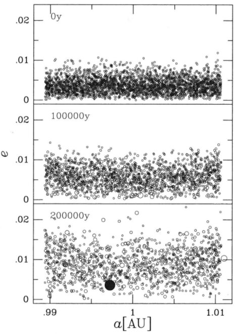
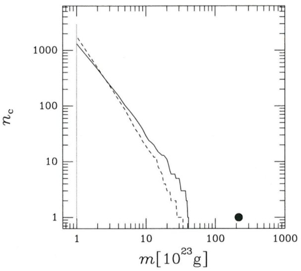
Figure 9: Example of the runaway growth process from planetesimals to planetary embryos using the $N$-body method as described by Kokubo 2001RvMA...14..117K . The basic setup and initial conditions are given in the main text in section 3.2. The left panel shows the eccentricity and distance distribution of the bodies for the initial setup (top panel) and at times 100,000 and 200,000 yrs (middle and bottom). The right panel shows the cumulative mass distribution of the formed bodies where $n_{\rm c}(m)$ = number of particles with mass larger than $m$. The results are shown at the same times as in the left panel: $t=0$ (vertical thin line), $t=100,000$ (dashed) and $t=200,000$ (solid). The large bullet in both panels denotes the single outstanding large object that has formed through a runaway process. From E. Kokubo 2001RvMA...14..117K

An illustrative example

To be specific, we present in the following an example for the typical outcome of the planetesimal growth process. In 2006expl.conf..369C representative results of the second (statistical) type of approach have been described in more detail 1993Icar..106..190W ; 1997Icar..128..429W and we refer the reader to that excellent summary. For a complementary point of view, we summarize here results of the $N$-body approach, that has been used for example by E. Kokubo 1998Icar..131..171K ; 2002ApJ...581..666K to describe planetesimal growth. In 2001RvMA...14..117K the main results of such simulations are presented, and we give here a short summary. Initially a number of planetesimals are spread over certain region around the central star, here the Sun, typically centered at $1$AU with certain radial width. In 2001RvMA...14..117K a radial extent of 0.02 AU, centered a $a=1$ AU, was chosen. The simulations used 3000 bodies, each with an initial mass of $m=10^{23}$g. The mean material density of the growing planetesimals was assumed to be $\rho_{\rm p}=2$g cm^-3. The whole ensemble was evolved in time for several 100,000 yrs.

As shown in Fig. 9, starting from the set of equal mass particles, at time $t=200,000$yrs the distribution has evolved towards the situation where one large body (the $\bullet$) has formed which has about 200 times the initial mass. It is embedded in a sea of smaller particles that have a continuous mass distribution, see right panel in Fig. 9. The low eccentricity (and inclination) of ($\bullet$) comes through dynamical friction with the small objects. Through (distant) gravitational interactions the smaller particles are dynamically excited, and their mean $e$ and $i$ increase in time. Using equipartition of energy between $e$ and $i$ yields on average the following relation $<e^{2}>=4<i^{2}>$ where $<x>$ denote mean values averaged over the ensemble of small particles. The one large object orbits the star on a nearly circular orbit.

For the same $N$-body simulation, the right panel in Fig. 9 shows the cumulative particle distribution, after $10^{5}$yrs (dashed), and after $2\times 10^{5}$yrs (solid). The objects between $10^{23}$-$10^{24}$g contain the majority of mass of the whole sample. The distribution follows a power-law

$$\frac{dn_{\rm c}}{dm}\propto m^{q}\,.$$ (28)

Here, $q$ describes the exponent of the power-law mass distribution, where a value of $q=-2$ is equivalent to equal mass in each logarithmic mass bin. A steeper distribution, $q<-2$, is characteristic for a runaway process 1993prpl.conf.1061L , where only very few particle reach larger masses. Indeed, in the simulation shown in Fig. 9 the slope is about $q\approx-2.7$ and one very massive particle ($\bullet$) is separated from the continuous distribution, i.e. it serves as a sink of particles. These results indicate very clearly that in the early phase the planetesimal growth proceeds through a runaway phase.

Very similar results to those shown in Fig. 9 are obtained for example by 1993Icar..106..190W and 1997Icar..128..429W using the statistical method, see summary in 2006expl.conf..369C . Their distribution of particle sizes follows a very similar slopes to that shown in the right panel of Fig. 9, again indicative of runaway growth.

The end of the growth

Obviously a runaway process, as just described, cannot continue forever. It is slowed down and eventually stopped mainly by two processes. Upon growing to larger objects the planetesimals stir up their environment such that the velocity dispersion is increasing and hence the relative velocity between them which leads, according to eq. (12) to a reduction in the collisional cross section. Secondly, the accretion process reduces the local density of particles, $\rho_{\rm part}$, and the body isolates itself from further growth, because fewer and fewer collision partners are available within the feeding zone. One can get an estimate on the final size an embryo can reach, the isolation mass $M_{\rm iso}$, by assuming that the volume of accretion, the feeding zone, has a radial extend given by the width of the horse shoe region, which is approximately given by the Hill-radius (17). The total mass of all the particles within a region $\Delta a$ inside and outside of semi-major axis $a$ is given by $m=2\pi\,2a\,\Delta a\Sigma_{\rm part}$. Using now $\Delta a=CR_{\rm H}$ we obtain with $m=M_{\rm iso}$

$$M_{\rm iso}=4\pi a\,C\,\left(\frac{M_{\rm iso}}{3M_{\odot}}\right)^{1/3}\,a\Sigma_{\rm part}\,,$$ (29)

where $C$ is a factor of order unity 2010apf..book.....A .

We consider now for example the growth of the Earth in the Solar System, and assume that there were initially $2M_{\oplus}$ located between $0.5$ und $1.5$AU. Using the standard condition of the MMSN with $\Sigma_{\rm part}\sim a^{-3/2}$ and $\Sigma_{\rm part}=8$ gcm^-3 at 1AU and $C=1$, then we obtain for the isolation mass

$$M_{\rm iso}\approx 0.05M_{\oplus}\,.$$ (30)

This runaway process is essentially a local phenomenon, because the embryos accrete primarily from their immediate neighborhood, their feeding zone. The limited extend of each embryo’s feeding zone implies that several objects in the protoplanetary nebula will experience runaway growth and grow at a similar rate. This is the oligarchic phase of terrestrial planet formation which results eventually in about 40 planetary embryos which have a mean spatial separation of about $\approx 0.01-0.025$AU 1987Icar...69..249L ; 2004E&PSL.223..241C . The timescale for this growth of the oligarchs is about 0.1-1.0 Myr 1997Icar..128..429W ; 2003Icar..161..431T . Due to the locality of the runaway growth, any radial compositional gradient present in the protoplanetary disk should be reflected in the embryos’ chemical compositions 2012AREPS..40..251M . Starting from these protoplanets the final assembly of the terrestrial planets can ensue.

3.3 Assembly of the terrestrial planets

After the oligarchic phase there are only a few objects, the embryos, left over with masses of about Moon to Mars size. The sea of planetesimals has mostly been depleted and only the gravitational interaction between these planetary embryos remains, i.e. in contrast to the previous growth phases the problem is physically relatively clean. To model this final assemblage, classical $N$-body simulations are the standard choice. In principle this is a straight-forward exercise because there are only very few particles ($\approx 100$) left over whose motion needs to be integrated, but this process occurs over a very long time scale, about $10^{7}-10^{8}$ yrs. Hence, the longterm integration of the equations of motion (similar to eq. 23 with vanishing gas and collision terms) requires good symplectic integrators that conserve automatically the total energy of the system. A well known, and often used example is the MERCURY-code developed by J. Chambers 1999MNRAS.304..793C which is publicly available. Other codes are for example the SWIFT-package 1998AJ....116.2067D or the REBOUND-code 2012A&A...537A.128R , a modern $N$-body code, with the capability to treat collisions.

As an example we discuss briefly the results of Chambers et al. 1998Icar..136..304C ; 2001Icar..152..205C . The authors performed a series of $N$-body simulations, where as starting conditions they used about 50 embryos in the first paper 1998Icar..136..304C and about 155 embryos in the second paper 2001Icar..152..205C . In total about 2 $M_{\oplus}$ were distributed between 0.3 and 2.0 AU with different types of initial mass distributions: all equal, bimodal or with a radial mass profile. In all simulations Jupiter and Saturn were included on their present day orbits. The collisions were treated as 100% sticking (perfectly inelastic) and the angular momentum of the coalesced bodies went into their spin. The presence of Jupiter and Saturn may be surprising at this still early phase during the growth of the terrestrial planets but, as we shall see in the following chapter, the formation timescale for these massive planets is indeed shorter than the time necessary for the final assembly of the terrestrial planets.

The results of those type of simulations show that indeed planetary system containing several terrestrial planets are produced. The formation timescale is a few $10^{7}$ years, which is very long compared to the previous phases. The reason is the fact that in this final growth phase only very few objects are remaining which reduces the frequency of mutual collisions considerably and it takes a long time to produce full grown terrestrial planets. The presence of the massive planets Jupiter and Saturn is required as they dynamically stir up the sample of embryos and prevent the formation of an additional planet within the region of the main belt asteroids. The whole evolution is a highly chaotic process because objects from different regions are scattered around and lead to a variety of collisions starting from head-on to near misses. Many objects may be lost as they fall into the Sun, and it is estimated 2001Icar..152..205C that about 1/3 of the initial objects within 2 AU may have to fear this fate. The typical outcome of these $N$-body simulations is a system with 3-4 planets on stable well separated orbits, with the tendency for more planets in those runs that have more initial embryos. Hence, the final systems in these simulations resemble roughly the situation in the Solar System where the most massive planets are in the Venus-Earth region, while the innermost planets and those in the Mars region are on average much smaller. The smallness of the Mercury type objects can be understood in terms of the high collision speeds for this innermost orbits that often lead to fragmentation rather than growth. Indeed the smallness and high density of Mercury can be attributed to a high speed impact during this chaotic phase of terrestrial planet formation 2007SSRv..132..189B . Most of the objects initially residing within the main asteroid region are scattered out due to resonant action by Jupiter and Saturn 2006Icar..184...39O .

Nevertheless there are important differences when compared directly to the Solar System: the mass concentration in the planets is not as high as for Venus and Earth, the planets have on average too high $e$ and $i$, and the spin-orientations are arbitrary. Specifically, the typical mass of a ’Mars’-object turns out to be too large when compared to the Solar System, by a factor of about 5. The presence of residual gas from the protoplanetary disk will reduce the eccentricities of the growing objects and shorten the formation time but too much gas will lower the collision rates such that massive planets like Venus and Earth will not form at all 2002Icar..157...43K . More recently, new evolutionary $N$-body simulations have been performed, some using a much larger number of initial bodies, a few thousand, that were spread over a wider radial domain ranging from 0.5-5.0 AU 2004Icar..168....1R ; 2006Icar..183..265R ; 2006Icar..184...39O . The influence of several input parameters to the simulations, such as the disk mass and radial density profile, the particle distribution in space and in mass, the orbits of the giant planets, and the treatment of collisions have been analysed in detail in more elaborate simulations, see overview in 2012AREPS..40..251M . From these one can infer that for the reduction of the orbital excitement of the terrestrial planets the dynamical friction of the remaining population of planetesimals plays an important role. Concerning the orbital architecture of the giant planets it was shown that for more eccentric giants the terrestrial planets grow faster and have more circular orbits 2009Icar..203..644R . While the overall architecture of the formed planetary systems resembles approximately the Solar System, the ’Mars-problem’ still remains. One scenario to overcome the problem of the too small Mars is the Grand Tack scenario where during the early Solar System the giant planets Jupiter and Saturn migrated first far inward and then turned around to move out to their present locations 2011Natur.475..206W . We will not discuss this scenario any further in contribution and refer the reader to excellent reviews 2012AREPS..40..251M ; 2014prpl.conf..595R .

The formation of terrestrial planets from planetesimals proceeds in different steps. In the first phase the gravitational attraction between the growing planetesimals leads to a fast runaway growth which is followed by a slower oligarchic growth phase, at the end of which an ensemble of about 50 Moon to Mars sized objects has formed, spatially well separated. On timescales of tens of millions of years these planetary embryos evolve under their mutual gravitational force and form through a sequence of collisions and impacts terrestrial type planets and the cores of giant planets.

4 The formation of massive planets by core accretion

In this section we describe how the growth of massive, gaseous planets is believed to proceed. The massive planets of the Solar System are about 100 times (Saturn) or 300 times (Jupiter) more massive than the Earth, which is the most massive object in the terrestrial planet region. Their mean densities are roughly comparable to that of water or even lower in the case of Saturn which implies that they consist of a huge amount of gas in addition to a possible central solid core. The question arises, how it is possible to collect large amounts of Hydrogen and Helium to form those planets under the conditions in the protoplanetary nebula. These lightest elements are highly volatile and difficult to condense. Two main pathways for the formation of massive planets have been discussed 2009ApJ...695L..53B .

In the first scenario, the core accretion model, an initial seed object forms onto which the gas can later accumulate. It is a bottom-up process, where initially a solid core forms along a similar evolutionary path as for the embryos in the formation of terrestrial planets. Upon reaching a certain critical mass the gravity of the core becomes high enough that a rapid, runaway gas accretion onto the core is possible, leading eventually to the formation of a gaseous planet. In the second scenario, the gravitational instability (GI) model, the formation pathway is similar to that of star formation and it is a top-down process. The scenario is believed to operate if the initial gas density of the protoplanetary disk is so high that a dynamical gravitational instability ensues that leads directly to the collapse of a local patch of the disk.

The physical structure of the gaseous planets in the Solar System has been studied extensively from the ground and through space missions. For the Solar System, the favored scenario is the core accretion model because it explains straightforward the existence of cores in the centers of the massive planets and the large amount of solids, with Jupiter enriched about $1.5-6$ times above solar composition and Saturn about $6-14$ times 2004ApJ...609.1170S . Additionally, the atmospheres of Saturn and Jupiter are enriched in metals and in noble gases, in particular Argon 2014arXiv1405.3752G . The formation via the GI process may have operated in the creation of the observed distant, directly imaged extrasolar planets. In this section we first focus on the core accretion pathway, while the GI model will be discussed below in the next section 5. The status of knowledge about the internal structure of the Solar and the extrasolar giant planets are reviewed in 2010SSRv..152..423F and recently in 2014arXiv1405.3752G . A classic review of this phase of planet formation is presented in 1993ARA&A..31..129L , while modern reviews are given in the relevant chapters of the Protostars and Planets series, here in PPVI 2014prpl.conf..643H ; 2014prpl.conf..619C .

4.1 Background

Planetary growth in the core accretion model consists of three phases. In the first phase a solid object forms in a manner similar to the processes that have led to the planetary embryos in the case of the terrestrial planets. In the previous section we have analysed the isolation mass of a growing body which is given by the amount of solid material that can be accreted directly from the feeding zone of an embryo. In contrast to the terrestrial region of the protoplanetary disk the abundance of solids is much higher at the location of Jupiter because of the low temperatures in the disk which allows for the condensation of many additional molecules, most importantly water. H₂O is the most abundant molecule in the Universe and in the disk it freezes out to ice beyond the so-called snowline. The exact condensation temperature depends on the ambient gas pressure but for conditions in the protosolar nebula $T$ has to be smaller than $(150-170)$K for ice to condense. For a passively heated disk where the stellar irradiation dominates the heat input to the disk, one finds for a Solar type star $r_{\rm cond}\approx 2.7$AU  for the condensation radius. Hence, in the standard Hayashi-model of the protosolar nebula, for distances to the star larger than $r_{\rm cond}$, the amount of solids available for embryo formation is typically assumed to be 4 times higher than in the inner regions 1981PThPS..70...35H . While newer calculations indicate possibly a lower value 2014A&A...570A..36M , we still use the standard value here, and then surface density for solids $\Sigma_{\rm s}$ is given by

$$\Sigma_{\rm s}(\mathrm{rock/ice})=30\left(r/1\mathrm{AU}\right)^{-3/2}\,\mbox{g/cm${}^{2}$ \quad for}\quad r>2.7\mbox{AU}\,.$$ (31)

Using the formula given in the previous section for the isolation mass we obtain at the current distance of Jupiter ($a_{\rm Jup}=5.2$AU) the following estimate

$$M_{\rm iso}\approx\,(5-9)M_{\oplus}\,,$$

which is considerably higher than in the terrestrial region. For the subsequent phases in the formation of giant planets the core mass is an important quantity, as it determines whether the embryo can capture a sufficient amount of gas in a short timescale to become a giant.

The first phase of gas accretion proceeds in a slow hydrostatic manner. The question arises: How much of an atmosphere can a growing planet hold? To answer this question, we assume that the minimum requirement for an atmosphere is that the escape velocity from the planet is larger than the sound speed in the ambient disk $v_{\rm esc}>c_{\rm s}$. In the discussion below we follow P. Armitage 2010apf..book.....A and use

$$m_{\rm p}=\frac{4\pi}{3}\rho_{\rm m}R_{\rm p}^{3},\quad\quad v_{\rm esc}=\sqrt{\frac{2Gm_{\rm p}}{R_{\rm p}}},\quad\mbox{and}\quad c_{\rm s}=\frac{H}{r}u_{\rm K}\,,$$

where $m_{\rm p},R_{\rm p}$ denote the mass and radius of the growing planet (embryo) with density $\rho_{\rm m}$, $v_{\rm esc}$ is the escape velocity from its surface, $c_{\rm s}$ is the sound speed and $H$ the vertical half-thickness of the disk. For an icy body at 5 AU around a Solar mass star we will have some atmosphere (where $v_{\rm esc}$ begins to be larger than $c_{\rm s}$) for $m_{\rm p}\,\gtrsim\,5\cdot 10^{-4}M_{\rm Earth}$. This is a very small mass planet, but such an atmosphere has no dynamical importance.

Let us consider the situation where the atmosphere or rather envelope takes up a sizable fraction, $f_{\rm env}$, of the planet such that $M_{\rm env}>f_{\rm env}\,m_{\rm p}$. For an isothermal atmosphere with $c_{\rm s}(atm)=c_{\rm s}(disk)$, and where the outer density matches that of the ambient disk ($\rho_{0}$) one obtains at $r=5\mbox{AU}$ with $\rho_{0}=2\cdot 10^{-11}$g/cm³, $c_{\rm s}=7\cdot 10^{4}$cm/s for the minimum mass of a planet to hold an atmosphere of about 10% of its mass ($f_{\rm env}=0.1$) 2010apf..book.....A

$$m_{\rm p}\gtrsim 0.2M_{\oplus}\,.$$ (32)

As a comparison, at the location of the Earth, one obtains for $f_{\rm env}=0.1$ at $r=1$AU using $\rho_{0}=6\cdot 10^{-10}$g/cm³, $c_{\rm s}=1.5\cdot 10^{5}$cm/s, and $\rho_{\rm m}=3$g/cm³

$$m_{\rm p}\sim M_{\oplus}\,,$$ (33)

in very rough agreement with the actual conditions in the Solar System. Planets are assembled over the life time of the disk and the mass of the embryo will be given by the isolation mass as defined in eq. (29). To hold an atmosphere, $M_{\rm iso}$ must be larger than the critical mass to acquire an atmosphere. An analysis 2010apf..book.....A shows that inside $r_{\rm cond}$ the isolation mass is always smaller than the mass to hold an atmosphere, while outside $r_{\rm cond}$ the isolation mass is larger. This relation explains qualitatively very well the fact that the inner planets in the Solar System consist of terrestrial planets with very little atmosphere while outside we find the gas or gas/ice giants with a very extended envelope. Further details will depend on the actual disk model, and the final location where gas giants are found eventually will depend on the amount of migration that occurred. To understand the final phase of the assembly of massive planets, we will have to study in more detail the internal structure of the growing giants.

4.2 The growth to a giant

To calculate the structure of a growing star or planet one assumes typically that the overall evolution of the mass growth proceeds on a timescale that is very long in comparison to the adjustment timescale of the interior. The latter can be estimated on the basis of the sound crossing time of an object that is of the order $\tau_{\rm cross}\sim(G\bar{\rho})^{-1/2}$, where $\bar{\rho}$ denotes the mean density of the body. For a growing planet $\tau_{\rm cross}$ is only a few minutes. Indeed, this is much smaller than typical accretion time scales, and the evolution of the growing planet can be well described by a sequence of hydrostatic models, similar to stellar evolution.

Hence, the basic equations that describe the inner structure of a growing planet are given by the standard stellar structure equations 1990sse..book.....K , adapted to the planet formation process 2005AREPS..33..493G

$$\mbox{\small mass conservation:}\hskip 28.45274pt\quad\frac{dm}{dr} = 4\pi r^{2}\rho$$ (34)

$$\mbox{\small hydrostatics:}\hskip 31.2982pt\quad\frac{dp}{dr} = -\frac{Gm(r)}{r^{2}}\,\rho$$ (35)

$$\mbox{\small radiative diffusion:}\hskip 19.91684pt\quad\frac{L(r)}{4\pi r^{2}} = -\frac{4\,\sigma T^{3}}{3\,\kappa_{\rm R}\rho}\,\frac{dT}{dr}$$ (36)

$$\mbox{\small energy generation:}\hskip 28.45274pt\quad\frac{dL}{dr} = -4\pi r^{2}\rho\left(\epsilon-T\frac{\partial S}{\partial t}\right)$$ (37)

with: $m(r)$ mass interior to the radius $r$; $L(r)$ luminosity at radius $r$; $\epsilon$ internal energy generation, $\sigma$ Stefan-Boltzmann constant, and $\kappa_{\rm R}$ Rosseland-opacity. Equations (34 - 37) are essentially the same equations as for stellar interiors with the difference that the luminosity is not due to nuclear burning of hydrogen but due to the contraction and cooling of the gas that changes the entropy $S$, as given by the last term in the energy equation. Impacting planetesimals give an additional contribution. In case of convection (for a super-adiabatic stratification) the adiabatic temperature gradient is used.

To calculate the structure of the whole planet, from the very center to the surface, equations of states for matter under extreme conditions are required. A simple estimate for the minimum central pressure, $p_{\rm c}$, can be obtained from the hydrostatic equation using the assumption of a constant density inside the body, $\rho(r)=\bar{\rho}$. Integrating eq. (35) then yields

$$p_{\rm c}=\frac{1}{2}\,\bar{\rho}\,\frac{GM}{R}\,,$$ (38)

where $M$ and $R$ are the total mass and radius of the planet. For the observed mass and radius of Jupiter ($M_{\rm Jup}=1.9\cdot 10^{27}$kg $=318M_{\rm Earth}$ and $R_{\rm Jup}=7\cdot 10^{7}$m $=11.2R_{\rm Earth}$) the mean density is given by $\bar{\rho}=1.33$ g/cm³, and eq. (38) gives $p_{\rm c}\approx 2.5\cdot 10^{12}$ Pa $=2.5\cdot 10^{7}$ bar. This result shows that to describe the interior structure of (massive) planets the conditions of matter under extreme conditions has to be known.

The obtained result for Jupiter’s $p_{\rm c}$ is slightly beyond that what present day experimental setups can reach (about $0.6\cdot 10^{12}$ Pa in diamond anvil cells 2012NatCo...3E1163D ), and due to the assumption of constant density the estimated value is the minimum $p_{\rm c}$ that Jupiter can have. Hence, the equations of state (EOS) that can be used to describe the inner cores of giant planets are constructed through a combination of theoretical calculations and experimental results. A summary of frequently used EOS is presented in 2010SSRv..152..423F , see also 2014prpl.conf..763B .

A simple equation of state used for the outer regions (envelope and atmosphere) is given by the ideal gas law

$$p=\frac{R_{\rm gas}\,\rho T}{\mu}\,,$$ (39)

with the gas constant, $R_{\rm gas}$, and the mean molecular weight, $\mu$, in units of $m_{\rm H}$.

To solve the structure equations (34 - 37) for a growing planet suitable boundary conditions have to be chosen. These are now different from the standard conditions of stellar growth because the planet is still embedded in the protoplanetary disk that acts as a mass and heat reservoir.

The inner boundary is given in this situation not by the central values but rather by the size and luminosity of the core. The size, $R_{\rm core}$, is given by solving the structure equations for the core for a given composition and core mass, $M_{\rm core}$. As a first approximation a constant density can be chosen for the core. The luminosity, $L_{\rm core}$, has different contributions. The main part comes from the residual kinetic energy of the accreted planetesimals after they have fallen through the envelope and land on the core. Additional core luminosity comes from radioactive decay in the core, core contraction and cooling of the core.

The outer boundary conditions at the planet’s radius, $R$, depend on the evolutionary status of the planet and the ambient disk. Mainly 3 different options have been considered 2015IJAsB..14..201M
1) Attached or nebular phase:
For small masses ($M$ lower than about 10-20 $M_{\rm Earth}$) the protoplanet is still deeply embedded in the disk such that its radius is much smaller than the disk scale height, $H$. Hence, its envelope is smoothly attached to the nebula. The planet’s radius in this case is given by the smaller of the accretion radius, $R_{\rm A}=GM_{\rm p}/c_{\rm s}^{2}$, and the Hill radius, $R_{\rm H}=(M_{\rm p}/3M_{*})^{1/3}a_{\rm p}$ (eq. 17), where a smooth transition is used between these two values. The accretion radius is half of the Bondi-radius which is often used in spherical accretion problems. The temperature and pressure at the outer radius, $R$ are then identical to the disk temperature at that location.
2) Detached or transition phase:
For larger masses, no solution satisfying the attached state exists, and the proto-planet contracts to a radius much smaller than $R_{\rm H}$. The luminosity follows from radial infall, via a spherical accretion shock, or through accretion from a circumplanetary disk 2005A&A...433..247P . The gas accretion is not anymore determined by planet, but by nebula conditions. For the spherical case the pressure at the surface is determined by the accretion shock (gas in free-fall) at the photospheric pressure. In reality the accretion onto the planet will not be completely spherical symmetric anymore and mass will be accreted through an accretion disk around the planet, the circumplanetary disk. Numerical simulations 1999MNRAS.303..696K ; 1999ApJ...526.1001L show that accretion occurs via 2 ’streams’ that are the extensions of the spiral shock waves generated by the planet that extend all the way into the Hill sphere of the planet, see Fig. 12. High resolution three dimensional simulations of the flow near growing planets show that a substantial amount of material is accreted through the polar regions 2003ApJ...586..540D ; 2014ApJ...782...65S .
3) Isolated or evolution phase: the planet evolves at constant mass and receives irradiation from central star that is spread over the whole planetary surface. The albedo of the planet is required for an accurate determination of the absorbed radiation. The photosphere is given, as in stellar models at an optical depth, $\tau=2/3$.

For the case where the luminosity is provided by the accretion of planetesimals the planetesimal-envelope interaction during the infall is crucial for the energy and mass deposition profile in the envelope. To determine the trajectory of infalling particles one has to consider first the gravity and gas drag (i.e. the envelope increases the capture radius of the growing planet), and the secondly thermal ablation and aerodynamical disruption. A modern example of this process is given by the infall of the comet Shoemaker-Levy 9, where temperatures over 30,000 K were reached in the bow shock around the infalling body. This interaction with the envelope will heat up the planetesimal that re-radiates this energy and will loose some of its mass, and may eventually disintegrate. The accumulation of energy by the envelope or core during these processes will determine the time evolution of the planet.

When performing evolutionary simulations of growing planets one extremely important finding was the fact that beyond a critical value of the core mass, $M_{\rm crit}$, the envelope cannot be in hydrostatic equilibrium anymore and will collapse onto the core 1974Icar...22..416P ; 1978PThPh..60..699M ; 1980PThPh..64..544M . This finding has given rise to the term core-instability model, sometimes also called core-accretion scenario. In the simulations, the hydrostatic equations stated as above were solved, where it was assumed that all planetesimals reach the core and provide the luminosity, $L_{\rm core}$, hence in the envelope $L(r)=const.=L_{\rm core}$. The critical mass, $M_{\rm crit}$, is a function of the opacity of the accreted material and it lies around $10M_{\rm Earth}$ for typical ISM composition. Subsequent numerical simulations confirmed exactly these early results and the runaway mass accretion is now the cornerstone in the core-accretion scenario. Noteworthy, classic simulations for the in-situ formation of Jupiter in the Solar System are presented 1986Icar...67..391B ; 1996Icar..124...62P . More elaborate models on the formation of massive planets that include the effects of accretion through a circumplanetary disk have been formulated 2005A&A...433..247P ; 2012A&A...547A.111M , which have been incorporated into population synthesis models of planets. The latter article 2012A&A...547A.111M contains a very readable introduction to that field.

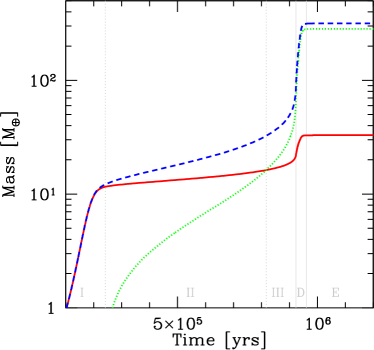
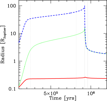
Figure 10: The evolution of the mass and radius of Jupiter in the Solar Nebula. During the whole growth the planet was fixed at its present position (in-situ formation). The core mass (made of solids) is given by the red line, the gas mass by the green line, and the total mass by the dashed blue line. The different phases of the accretion process have been marked by the vertical lines and additional roman numbers in the left panel, see text for more details. In the right panel, the red line refers to the core radius, the blue dashed line to the total radius, and the green line to the capture radius of planetesimals. Courtesy: Chr. Mordasini, see also 2012A&A...547A.111M

Initially difficult to understand the physical mechanism of the core-instability process, Stevenson 1982P&SS...30..755S presented a simple analytical model of the process, that helped to uncover the underlying principles, and that is summarized nicely in 2010apf..book.....A . For typical parameters in the protosolar disk one obtains 1982P&SS...30..755S

$$M_{\rm crit}\simeq 20\kappa_{\rm R}^{3/7}\,M_{\oplus}\,,$$ (40)

where $\kappa_{\rm R}$ denotes the Rosseland mean opacity in units of [cm²/g]. For $M_{\rm core}>M_{\rm crit}$ the core contracts rapidly and runaway gas accretion sets in. Full numerical simulations are required to obtain the exact evolution of this phase that includes the details on the boundaries as given above in particular the contact with the ambient disk and the solid particle accretion process.

An example of such a calculation for the in-situ formation of Jupiter in the Solar nebula 2012A&A...547A.111M is shown in Fig. 10. The vertical lines and roman numbers indicate different evolutionary phases: I-III) refer to the attached phase with the protoplanet in contact with the disk, where I) denotes the assembly of the core, II) refers to the the continued slow core accretion and hydrostatic gas accumulation, isolation of solid particles, and in III) the core reaches the critical mass with the onset of rapid gas accretion. D) is the detached phase, and E) the long term isolation, or evolution phase. The authors 2012A&A...547A.111M point out that the depicted evolution serves as a test case that was described very similarly in early simulations 1986Icar...67..391B ; 1996Icar..124...62P . The overall evolution indicates that the typical time scale to form Jupiter is about a million years. However, there are many factors that have an impact on the overall evolutionary timescale. Details will depend on the:

• Opacity
  Low values of $\kappa_{\rm R}$ will allow faster envelope growth. It it determined essentially by the amount of dust present in the envelope because the gas opacities alone are much too low.

• Convection
  The onset of convection in the envelope will enhance the efficiency of energy transport and hence change the time scale for accretion.

• Chemical composition
  The chemical composition influences the opacity and the mean molecular weight, $\mu$. The latter has through the equation of state (39) a direct impact on the pressure and hence the radial stratification through the requirement of hydrostatics.

• Accretion rate
  The accretion onto the core, $\dot{M}_{\rm env}$, is often estimated from one-dimensional models. However, only through two-dimensional (circumplanetary disk) and three-dimensional simulations (polar accretion) can the actual accretion rate been obtained.

• Migration
  The migration of the growing planet through the disk has an influence on the mass accretion rate. For example, new reservoirs for the solid particle as well as gas accretion will be opened.

One very important ingredient in determining the overall growth time scale is the formation time of the core, which is determined by the accretion of solids from the disk. Obviously this is directly proportional to the solid particle density in the disk, $\Sigma_{\rm solid}$. The simulations indicate that for $\Sigma_{\rm solid}<10$g/cm² the time scale for core formation is too long such that the gas reservoir of the disk will also be depleted given the typical disk lifetime of a few million years. On the other hand, for $\Sigma_{\rm solid}>10$g/cm² there are too many heavy elements in comparison to today’s Jupiter composition. Given that the surface density of solids for the MMSN is only 5 g/cm² (at the location of Jupiter), there appears to be a timescale problem in that the growth time for the core formation is too long for Jupiter, and the problem becomes even more severe in case of Uranus and Neptune formation.

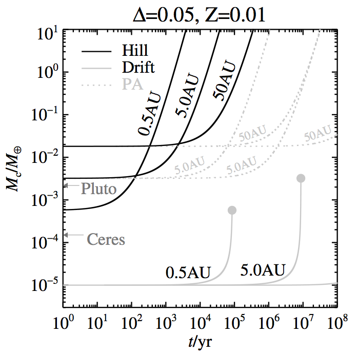
Figure 11: The growth of a planetary core as a function of time at different radii in the disk. Curves are shown for the Hill regime ($m_{\rm p}<M_{\rm t}$, with the transition mass $M_{\rm t}$, see eq. 41), the drift regime ($m_{\rm p}>M_{\rm t}$) and the standard pebble accretion (PA). The result shown are for a headwind parameter $\Delta\equiv\Delta v_{\rm K}/c_{\rm s}=0.05$ (see eq. 42) and a dust to gas mass ratio $Z\equiv\Sigma_{\rm p}/\Sigma=0.01$. Taken from 2012A&A...544A..32L

A new option that is presently discussed in more detail is the idea to enhance the growth of planetary cores by rapid accretion of small pebbles 2012A&A...544A..32L . In contrast to the larger planetesimals, these typically cm to dm-sized particles feel the gas drag. When pebbles approach a growing core which has some atmosphere already collected within its environment, the gas drag will slow them down and they will spiral deeper into the Hill sphere towards the planet and become eventually accreted by it. Depending on the mass of the growing core two different types of accretion regime can be distinguished 2012A&A...544A..32L . First we define a Bondi-radius for the growing object as $R_{\rm B}=GM_{\rm p}/\Delta v_{\rm K}$, where $\Delta v_{\rm K}$ is the velocity difference between the Keplerian rotation and particle speed due to the gas drag. By equating the Bondi-radius and the Hill radius one can define a transition mass, $M_{\rm t}$, where both are equal. For the MMSN one finds

$$M_{\rm t}\approx 0.016M_{\oplus}\,\left(\frac{r}{30AU}\right)^{3/4}\,\left(\frac{\Delta v_{\rm K}}{0.1c_{\rm s}}\right)^{3}\,.$$ (41)

For $m<M_{\rm t}$ ($R_{\rm B}<R_{\rm H}$) accretion occurs in the so-called drift regime, while for $m>M_{\rm t}$ (i.e. $R_{\rm B}>R_{\rm H}$) it occurs in the Hill regime. For the growth of massive planets the more interesting phase will be the Hill regime with $m>M_{\rm t}$.

Classically, the accretion rate of planetesimals onto a planetary core (100% sticking) is given by $\dot{M}_{\rm p}=\Sigma\Omega R_{\rm p}^{2}F_{\rm grav}$ 1987Icar...69..249L (see also eq. 22), where $R_{\rm p}$ is the planetary radius and $F_{\rm grav}$ the gravitational focusing factor (eq. 14). Since only a fraction $\alpha_{\rm p}=R_{\rm p}/R_{\rm H}$ of the whole Hill sphere is captured for a growing core 2004ARA&A..42..549G ; 2012A&A...544A..32L , the mass accretion will be changed to $\dot{M}_{\rm p}(\text{planetesimals})=\Sigma\Omega\alpha_{\rm p}R_{\rm H}^{2}F_{\rm grav}$. On the other hand, since pebbles feel the gas drag, all objects that reach the Hill sphere will be accreted and the accretion rate becomes $\dot{M}_{\rm p}(\text{pebbles})=\Sigma\Omega R_{\rm H}^{2}F_{\rm grav}$. Clearly, for a growing core with $m>M_{\rm t}$, the Hill radius will be much larger than its actual, physical radius, such that $\alpha_{\rm p}\ll 1$. Then the ratio $\dot{M}_{\rm p}(\text{pebbles})/\dot{M}_{\rm p}(\text{planetesimals})$ will be much larger than unity, reducing the accretion time scale for the core considerably. Indeed, the simulations of Lambrechts & Johansen 2012A&A...544A..32L show that under the assumption of a steady influx of new material (from outside) and pebbles well settled to the midplane of the disk, the growth time for a 10 $M_{\rm Earth}$ core is less than $10^{5}$ yrs at 5 AU, and less than $10^{6}$ yrs at 50 AU, see Fig. 11. Clearly, these growth times are much shorter than those expected by pure growth of planetesimals and would ease the timescale problems for massive planet formation considerably. The exact efficiency of this problem will depend on several physical mechanisms, such as the so-called headwind parameter

$$\Delta=\Delta v_{\phi}/c_{\rm s}\,,$$ (42)

the vertical pebble concentration, $Z=\Sigma_{\rm p}/\Sigma$, a possible migration of the core and of course the structure of the envelope within the Hill sphere of the planet. In eq. (42) $\Delta v_{\phi}$ is the velocity difference between the pebbles, which have a Keplerian velocity, and the gas in disk that moves slower due to the radial pressure gradient. The details need to be worked out, and also the question how the formation of lower (Neptune) mass planets fit into this new model.

4.3 The final mass

In the previous section we have seen that in the final stages the planet grows in a runaway fashion, and the question arises what determines the final mass of a planet. The simplest answer to this might be fact that the amount of gas that is available in the disk is necessarily finite which sets eventually a natural mass limit. While the limited mass reservoir in the disk certainly plays a role, there is an important additional factor that does inhibit mass growth, and this is the opening of a gap. We might expect that when the Hill radius of the planet exceeds the vertical scale height of the disk, $R_{\rm H}\gtrsim H$, this will have a significant impact on the disk structure, and alter the mass accretion rate. We will analyse this from two perspectives, a particle based approach and a hydrodynamical one.

In the first particle approach, the velocity change experienced by an individual (gas) particle that passes by a growing planet in the disk can be calculated most easily in the impulse approximation 1979MNRAS.186..799L . Here, it is assumed that the motion of the particle is primarily Keplerian in most part of the orbit and only perturbed in the vicinity of the planet. This creates an additional gravitational force (impulse) on the particle that leads to a deflection of its trajectory and a slight change in its azimuthal velocity, and hence angular momentum. Due to the collisions with other nearby disk particles this angular momentum change is immediately ’shared’ between them. Integrating the angular momentum exchange over all particles, i.e. over the whole disk, one can calculate the total rate of angular momentum input to the disk mediated by the planet

$$\dot{J}_{\rm grav}=-\frac{8}{27}\left(\frac{r_{\rm p}}{\Delta r_{0}}\right)^{3}\left(\frac{m_{\rm p}}{M_{*}}\right)^{2}\,\Omega_{\rm p}^{2}\,\Sigma(r_{\rm p})\,r_{\rm p}^{4}\,,$$ (43)

where $r_{\rm p}$ denotes the distance of the planet from the star, $\Delta r_{0}$ is the closest approach of a disk particle to the planet, and the index $p$ denotes that all quantities are evaluated at $r_{\rm p}$. The minus sign indicates that the inner disk loses angular momentum while the outer gains it, i.e. in the planet region the disk will be ’pushed’ away from the planet, see below. In spite of the simple approximation is result nearly exact. A nice pedagogical treatment of the derivation is given in the lecture notes of the Saas-Fee Advanced Course 31 by P. Cassen 2006expl.conf..369C . From eq. (43) it is clear that in the vicinity of planet ($\Delta r_{0}\rightarrow 0$) there is a strong increase of $\dot{J}$, and the total amount deposited will depend on the choice of $\Delta r_{0}$.

In the second hydrodynamic approach, the continuum behaviour of the gas in the disk is analyzed and the angular momentum deposition follows from more complex wave phenomena. A planet embedded in a disk produces disturbances in the disk’s density distribution. These are sound waves that spread out from the planet’s position because its presence impacts the dynamics of the ambient gas. The Keplerian shear flow in the disk turns these sound waves into a spiral wave pattern with an outer trailing arm and an inner leading one, as shown in Fig. 19 below. The spiral wave pattern is stationary in a frame corotating with the planet and hence, at a certain radial distance from the planet they reach a supersonic speed with respect to the Keplerian disk flow. At this point the waves turn into shock waves, dissipate energy and deposit angular momentum to the disk. In the outer disk the spiral arm is faster than the disk material and it deposits positive angular momentum, i.e. the outer disk material gains angular momentum and hence speed, and moves away from the planet, because in a Keplerian disk the angular momentum increases as $\propto r^{1/2}$. Inside of the planet the situation is reversed, the spiral arm is slower than the disk and negative angular momentum is deposited which leads to an inward motion of the disk material. In total, the disk matter is receding from the location of the planet lowering the density in its vicinity. The effect increases with planet mass and eventually an annular gap in the density is formed at the location of the planet, which happens even without considering direct mass accretion onto the planet. This lowering of the ambient density decreases the available mass reservoir and the gas mass accretion onto the planet will be reduced accordingly.

From eq. (43) it is clear that the deposition rate of angular momentum will increase with the mass of the growing planet, and in the absence of other effects there will be no mass left at the planet location. However, there are two main competitors, viscosity and pressure, working against this continuing gap deepening. The viscous disk torques at the location of the planet are given by

$$\dot{J}_{\rm visc}=\dot{M}_{\rm disk}j_{\rm p}\,=\,3\pi\Sigma(r_{\rm p})\nu\,r_{\rm p}^{2}\Omega_{\rm p}$$ (44)

with the kinematic disk viscosity $\nu$ and the specific angular momentum of the planet, $j_{\rm p}=r_{\rm p}^{2}\Omega_{\rm p}$. In writing eq. (44) we have assumed a stationary accretion disk with a globally constant mass accretion rate 1981ARA&A..19..137P . The viscous criterion for gap formation is then $\dot{J}_{\rm grav}\geq\dot{J}_{\rm visc}$. If one assumes for the smallest distance the Hill radius (17) of the planet, $\Delta r_{0}=R_{\rm H}$, then

$$q\geq q_{\rm visc}\simeq\frac{10\nu}{\Omega_{\rm p}\,r_{\rm p}^{2}}\,,$$ (45)

where $q$ is the planet to star mass ratio, $q=m_{\rm p}/M_{*}$. A second, pressure criterion of gap formation is obtained from the condition that the Hill sphere of the growing planet is larger than the disk thickness, i.e. $R_{\rm H}\geq H$ which gives

$$q\geq q_{\rm Hill}\simeq 3\left(\frac{H}{r}\right)^{3}_{\rm p}\,.$$ (46)

For typical parameter of the protoplanetary disk both criteria yield similarly a limiting mass for gap formation between Saturn and Jupiter. This explained the mass of Jupiter in the Solar System quite well. Using two-dimensional hydrodynamical simulations a more general criterion for gap formation has been derived 2006Icar..181..587C

$$\frac{3}{4}\frac{H}{R_{\rm H}}+\frac{50}{q\,Re}\leq 1\,,$$ (47)

with the Reynolds number $Re=r_{\rm p}^{2}\Omega_{\rm p}/\nu$. This last criterion assumes that the density of the disk at the location of the planet has been reduced to 10% in comparison to the unperturbed disk density. Additional, new estimates on the depth and width of the gap have been developed more recently, they will be discussed in more detail in section 6 below.

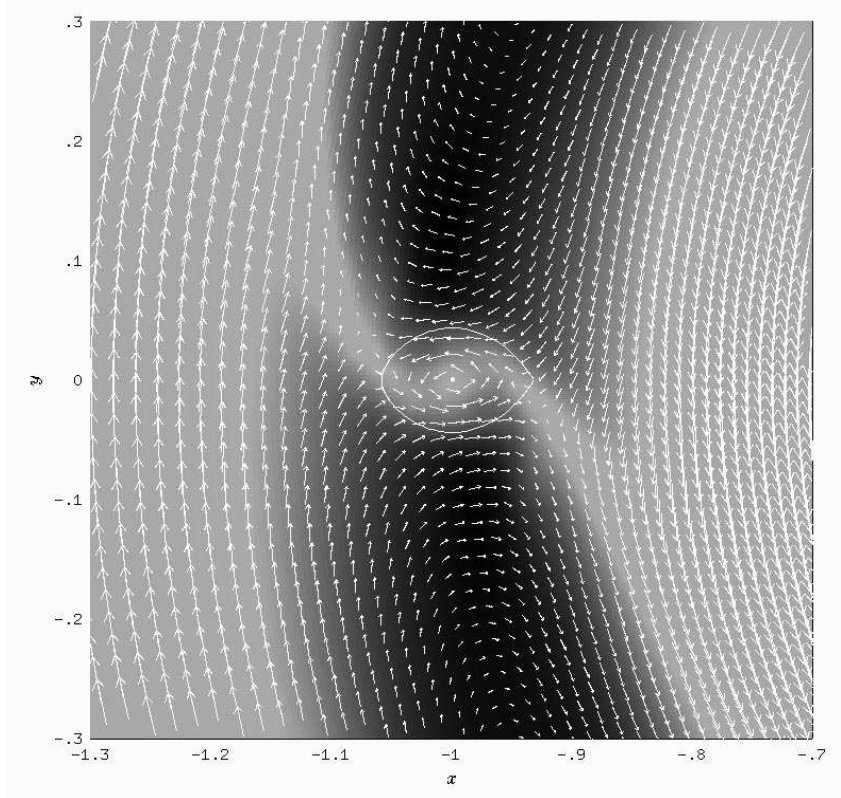
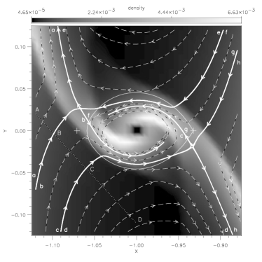
Figure 12: The gas flow around a Jupiter type planet embedded in a protoplanetary disk. The planet is at location $x=-1,y=0$ (in units of $5.2$ AU), and the star is located at the origin. Both panels show a density image (in Cartesian coordinates) of the Roche lobe region near the planet. The motion of the planet around the star would be counter clockwise in an inertial frame of reference. Left) The flow field around the planet, displayed in a reference frame corotating with the planet. The solid white line indicates the Roche lobe of the planet. Taken from 1999MNRAS.303..696K . Right) Density contours with sample streamlines given by the dashed lines. The left (right) plus sign marks the L2 (L1) point. Critical streamlines that separate distinct regions are the solid white lines. Material approaching the planet within these critical lines (i.e. between ’b’ and ’c’ on the outside, and between ’f’ and ’g’ on the inside) can become accreted onto the planet, while material at the outside (or inside) either circulates or enters into the horseshoe region and crosses it. Taken from 1999ApJ...526.1001L .

The finding that the mass of Jupiter coincides with the mass required to open a significant gap in the disk has often been taken as an indication that it is the gap creation that will eventually limit the final mass of a planet. This is after all in agreement with the fact that Jupiter is the most massive planet in the Solar System. However, the discovery of several extrasolar planets with masses much above Jupiter’s indicated that there must be a way to increase the mass even further in spite of the gap formation. Indeed, hydrodynamical simulations showed that the gap is not as impermeable as thought, because mass can enter the horseshoe region and either be accreted onto the planet or move from outer disk (beyond the planet) to inner disk or vice versa. The detailed flow field of the gas in the close vicinity of the planet is depicted in Fig. 12 for a Jupiter mass planet. Clearly, even though a clear gap has formed material can still be accreted onto the planet - the mass entering within the critical while lines on the right panel. For a Jupiter mass planet the mass accretion rate onto the planet is of the order of the equilibrium disk accretion rate, $\dot{M}_{\rm disk}=3\pi\Sigma\nu$ which leads to a doubling time of a few $10^{5}$ yrs for typical disk masses 1999MNRAS.303..696K . Increasing the mass from 1 to 6 $M_{\rm Jup}$ the accretion rate onto the planet drops by nearly one order of magnitude 1999ApJ...526.1001L . The results indicate that one Jupiter mass is not the limiting mass for planets in agreement with the observations, but beyond 5-6 $M_{\rm Jup}$ growth times become very long. Despite this apparent limitation, it turns out that further mass accretion is nevertheless possible because massive planets will induce a significant eccentricity in the outer disk such that periodically the planet will enter into the disk allowing for more mass accumulation onto the planet 2006A&A...447..369K .

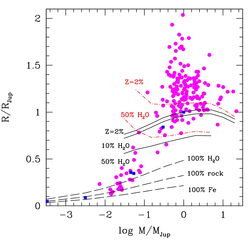
Figure 13: Mass versus radius of known exoplanets, including Solar System planets (blue squares, Mars to Neptune) and transiting exoplanets (magenta dots). The curves correspond to interior structure and evolution models at 4.5 Gyr with various internal compositions, and for a mass range in 0.1 $M_{\rm Earth}$ to 20 $M_{\rm Jup}$. The solid curves refer to a mixture of H, He and heavy elements, as indicated by the labels. The long dashed lines correspond to models composed of pure water, rock or iron from The ’rock’ composition here is olivine (forsterite Mg₂ SiO₄) or dunite. Solid and long-dashed lines (in black) refer for non-irradiated models while dash-dotted (red) curves correspond to irradiated models at 0.045 AU from a Sun. Taken from 2014prpl.conf..763B .

4.4 Interior structure of planets

After having studied the formation of planets let us very briefly comment on the information on the internal composition that can be drawn from the sample of observed exoplanets. The transit method allows for a determination of the planet’s radius, or at least the ratio of planetary to stellar radius, $R_{\rm p}/R_{*}$, because the reduction in flux during the transit is directly proportional to the square of this quantity. The Kepler mission allowed the determination of planetary radii for over thousand exoplanets and even from the ground there have been over 200 transit detections. To know in addition the mass of the planet, the radial velocity signal is required. Unfortunately, this has only been possible for a small fraction of the Kepler planets but for many of the ground based transit detections. Knowing the mass and radius of the planet, the mean density of the planet is determined and rough estimates as to its composition can be made. The important mass-radius (M-R) diagram can be constructed and compared to the theoretical models for the planet interiors. To calculate the interior models the structure equations as written above (34 - 37) need to be solved for long evolutionary times, after the disk has dispersed. What determines the final radius of a planet with a given mass is primarily its composition. Different constituents directly alter the mean density and will determine the important equation of state (EOS), that relates pressure to density (and temperature). Hence, the EOS defines the compressibility of the material and has direct influence on the planetary radius. The second factor is the age of the planet, as this determines the remnant heat that is still incorporated within and has not been lost by some cooling process. A third factor is the distance from the star as this determines the amount of external heating that is received by the planet for example by direct irradiation from the central star or the strength of the tidal interaction and dissipation.

In order to obtain accurate models, details of additional physical processes have to be considered that are often not known very well. The equation of state has to be known within a regime up to about 20,000 K and 70 Mbar which is only partly accessible by experiments. Shock-wave and compression experiments give only data up to a few Mbar, and theoretical calculations based on Quantum Molecular Dynamics simulations have to be performed in addition. Knowledge about possible phase transitions has to be acquired. For the cooling rate of planets the amount of radioactive elements need to be known, the efficiency of convection or plate tectonics (viscosity of the material) to be determined. For a recent summary of the present status of the field see the PPVI review 2014prpl.conf..763B , where Fig. 13 is taken from. In the figure, the $M-R$ diagram is shown for a sample of detected transiting exoplanets and some Solar System planets together with calculated theoretical curves. Because the transit probability increases strongly with shorter periods, i.e. shorter distances from the star, the exoplanets sample refers basically to ’hot’ planets.

As seen in the diagram, these can be divided in two major groups: hot Neptunes (Super-Earths) and hot Jupiters. The first group which is the actually most abundant in absolute numbers, as discovered by the Kepler-mission, is under-represented here due to the mentioned lack of radial velocity data of the Kepler planets. Clearly, as can be inferred from the reference objects in the Solar System, the locations of the points give indeed a good first indication of the composition of the planets, indicating that many of the Super-Earths may consist of rock and iron material while the Jupiter mass objects are gaseous planets that will consist primarily of Hydrogen and Helium. Sometimes very exotic options make it into the public media. One example is the so called ’diamond’ planet 55 Cnc e, for which some radius estimates indicated a value that matched exactly that of a planet with a composition of 100% diamond material. However, a mixture of carbon, silicates and iron material will match the observations equally well 2012ApJ...759L..40M . An additional feature that can be inferred from the Fig. 13 is that the majority of the hot Jupiter planets are much larger than predicted even if purely solar composition is assumed, i.e. they are inflated. Assuming irradiation from the star does indeed increase the radius somewhat but is by no means sufficient to explain the observed large radii. Observationally, it has been found that the amount of inflation decreases clearly with distance from the central star 2011ApJS..197...12D , implying that the central star is responsible for the effect. Possible suggested mechanisms are irradiation, tidal friction between the orbiting planet and the star during the circularization process of eccentric planets, or electrical currents generated through the interaction of ionized particles with the planetary magnetic field 2011ApJS..197...12D . However, the main cause is not known as of today.

Information drawn on the inner structure of the massive planets in the Solar System has given rise to the core accretion scenario of giant planets. Within this model, first solid cores of a few Earth masses are forming in a manner similar to the assembly of terrestrial planets. Once grown big enough, the ambient gas will be accreted onto the core, hence the terminology core accretion scenario. This evolutionary phase can be described by the classical stellar evolution equations augmented by suitable boundary conditions accounting for the fact that the planet is still embedded into the disk and the luminosity is created by the infall of solid material. As it turns out, once the core has grown to a critical mass, the gas accumulation proceeds in a runaway fashion such that on a timescale of a few million years a gas giant can be created at the location of Jupiter’s orbit. Going to larger distances from the star the evolutionary timescales (for core formation and gas accretion) become longer than the typical lifetimes of the disk. A solution to this timescale problem may be given by the pebble accretion scenario where solid, cm-sized particles are continuously accreted such that the critical core mass can be reached very fast, reducing the formation time significantly. Information on the interior composition can be obtained for transiting extrasolar planets if additional radial velocity data allow for a mass determination. The observations show that, due to star-planet interactions, most of the Jupiter type planets are significantly inflated in their radii.

5 Planets formed by gravitational instability

Having discussed the formation of planets via the core accretion (CA) scenario in the preceding section we will now turn to the alternative scenario of planet formation, the gravitational instability (GI) of the disk. While CA is the preferred scenario for the planets in the Solar System, GI is a possible a pathway considered for planets at large distances from their host stars. First, we will present observational examples of directly imaged planets that are indeed located at large distances from their host stars. Then we will consider the question under what conditions a disk can fragment directly to form planets. For such an analyses primarily two methods have been used. First a linear stability analyses and secondly full nonlinear numerical simulations of self-gravitating disks. We will describe the main findings below.

5.1 Background

The most prominent example of directly imaged planets is the system HR 8799 in the constellation Pegasus. For this system, in 2008 the detection of 3 planets was announced, discovered using adaptive optics at the Keck telescopes in Hawaii 2008Sci...322.1348M . The system was observed at different epochs such that the motion of the individual planets across the plane of the sky was detected. Hence, this discovery marks clearly a breakthrough in exoplanetary science because for the very first time the actual motion of planets around another star was directly detected, following the classical terminology of a planet being a ’wandering star’. Coincidentally, the position of this first directly imaged ’real’ planetary system in the sky lies very close to the first planet discovered by the RV method, 51 Peg. The system is observed nearly face on, and the observed motion of the planets agrees very well with the Keplerian motion about the host star that has a mass of $1.5M_{\odot}$. The 3 planets are 24, 38, and 68 AU away from the star and have estimated masses of $10,10$ and $7M_{\rm Jup}$. These masses are upper limits set by dynamical stability arguments where it must be assumed that they are engaged in a resonant configuration 2010ApJ...710.1408F . Later, in 2010 a fourth planet located at only 14 AU distance from the star was discovered 2010Natur.468.1080M . In Fig. 14 the layout of the whole planetary system HR 8799 is displayed. It is shown in a special scaling such that the similarities to the outer Solar System planets become apparent. Even the spatial distribution of the debris material is similar. So, one may speculate about the existence of terrestrial planets in that system. Otherwise there have only been a few systems where directly imaged planets in the few Jupiter mass range have been found, for example Fomalhaut b, $\beta$ Pictoris b or Gliese 504 b, even though the status of Fomalhaut b has been debated.

Despite these interesting similarities the large absolute distances of the planets in HR 8799 pose a challenge for their formation, due to severe timescale and stability problems. Comparing the effectiveness of various formation scenarios to form planets at large distances such as core accretion (with or without migration), outward scattering from the inner disk, or gravitational instability it was suggested that the last scenario is the most likely 2009ApJ...707...79D . For example, in the classical core accretion scenario the growth time of Neptune at its present orbit will be of the order 2010apf..book.....A

$$\tau_{\rm grow}=\frac{m_{\rm p}}{dm_{\rm p}/dt}\approx 5\cdot 10^{10}\,F_{\rm grav}^{-1}\quad\mbox{yr}\,,$$ (48)

where we assumed $\Sigma_{\rm part}=1$ g/cm³ in eq. (22). This is a very long timescale unless the gravitational focusing factor, $F$, is very large ($\sim 10^{4}$). Considering the larger distances of the planets in HR 8799 and the youth (60 million yrs) of the host star it appears unlikely that those planets have formed at these large distances by core accretion, although pebble accretion may help in this case (see above). And, since the formation via scattering often led to unstable systems it was concluded that formation via gravitational instability was the most viable mechanism to form the HR 8799 system 2009ApJ...707...79D , possibly related to later periods of mass fall-in from the envelope 2010ApJ...714L.133V . In models explaining HR 8799, the resonant structure of the planets places further constraints as it seems to require some migration process.

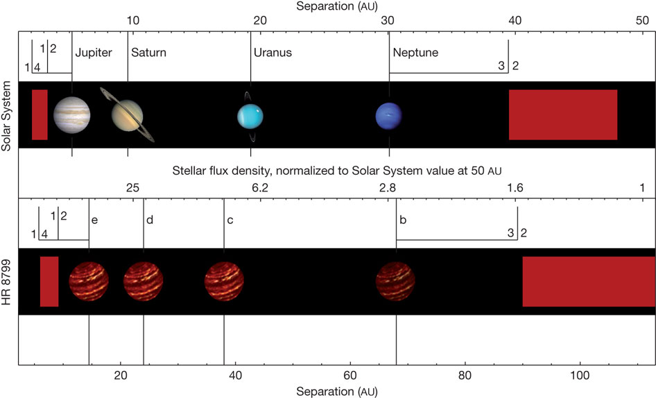
Figure 14: The structure of the planetary system HR 8799, that contains 4 massive planets all discovered by direct imaging, in comparison to the outer Solar System. The $x$-axis has been compressed according to the luminosities of the host stars by the factor $\sqrt{L_{\rm HR8799}/L_{\odot}}$, with $L_{\rm HR8799}=4.9L_{\odot}$. This means that the planets in HR 8799 are about two times farther away from the star but have the same equilibrium temperature as the Solar System planets because of the higher luminosity of the host star in HR 8799. The red rectangles indicate the regions where debris material is orbiting the stars. The lines marked with 1:4, 1:2 and 3:2 indicate the locations mean-motion resonances with respect to the planets. Taken from 2010Natur.468.1080M .

5.2 Linear stability analyses

To study the linear stability of a thin disk rotating around a central object we first assume that the disk is infinitesimally thin and follow the evolution in a two-dimensional setup. In the context of galactic dynamics, the classical studies are given by Toomre 1964ApJ...139.1217T and Lin & Shu 1964ApJ...140..646L , and a local shearing sheet analysis is presented in 1987gady.book.....B . To give an idea on how such a stability analyses is performed we sketch briefly the procedure. The set of hydrodynamical equations in cylindrical coordinates ($r,\varphi$) for a disk confined in the $z=0$ plane are given for example in 1998ApJ...504..945L and read

$$\frac{\partial\Sigma}{\partial t}+\nabla\cdot(\Sigma{\bf u})=0$$ (49)

$$\frac{\partial(\Sigma v)}{\partial t}+\nabla\cdot(\Sigma v{\bf u})=\Sigma\,r\Omega^{2}-\frac{\partial P}{\partial r}-\Sigma\frac{\partial\psi}{\partial r}$$ (50)

$$\frac{\partial(\Sigma r^{2}\Omega)}{\partial t}+\nabla\cdot(\Sigma r^{2}\Omega{\bf u})=-\frac{\partial P}{\partial\varphi}-\Sigma\frac{\partial\psi}{\partial\varphi}$$ (51)

where $P$ is the 2D vertically integrated pressure, $\vec{u}=(u_{r},u_{\varphi})=(v,r\Omega)$ the 2D velocity, and $\psi$ the gravitational potential

$$\psi=\psi_{*}+\psi_{\rm d}+\psi_{\rm p}\,,$$ (52)

that is given here as the sum of the stellar potential, $\psi_{*}=-GM_{*}/r$, the disk contribution

$$\psi_{\rm d}(r,\varphi)=-G\int_{\rm disk}\ \frac{\Sigma(r^{\prime})r^{\prime}dr^{\prime}d\varphi^{\prime}}{\sqrt{r^{2}+r^{{}^{\prime}2}-2rr^{\prime}\cos\varphi^{\prime}}}\,,$$ (53)

and possibly a planetary contribution, $\psi_{\rm p}$, that is neglected in this discussion. In eq. (53) the integration has to be performed over the whole disk. For the pressure we assume that it is given as a function of the surface density, $P=P(\Sigma)$, as is the case for the isothermal or adiabatic equations of state. To study the stability we start from an axisymmetric equilibrium state

$$r\Omega_{0}^{2}-\frac{1}{\Sigma_{0}}\frac{\partial P_{0}}{\partial r}-\frac{\partial\psi_{0}}{\partial r}=0\,,$$ (54)

where the subscript $0$ refers to the unperturbed basic state which is a function of the radius alone. Now the system is perturbed by adding a small perturbation

$$f(r,\varphi,t)=f_{0}(r)+f_{1}(r,\varphi,t)\,,$$ (55)

with $f\in\{\Sigma,v,\Omega,\psi\}$. Here, we only consider perturbations within the plane of the disk. The ansatz (55) is substituted into the full time dependent hydrodynamical equations (49) to (51) which are then linearized, i.e. two main assumptions are applied: a) The functions $f_{1}$ are assumed to be small compared to their equilibrium counterparts, i.e. $f_{1}\ll f_{0}$. This implies that terms that are quadratic in the perturbations $f_{1}$ can be neglected with respect their linear counterparts. b) The stratification of the background varies only slowly, which implies that the radial derivatives of the basic functions are assumed to be small in comparison to those of the perturbed functions, i.e. $\partial f_{0}/\partial r\ll\partial f_{1}/\partial r$. After these simplifications the non-linear hydrodynamic equations have been transformed into a set of linear equations for the perturbed quantities, that can in principle be integrated numerically. However, better insight is obtained by further analysis.

Because the basic state has neither a time nor an azimuthal dependence, one can quite generally expand the perturbations in a Fourier series

$$f_{1}=\tilde{f}_{1}(r)e^{i\left(m\varphi-\sigma t\right)}\,,$$ (56)

where $m$ denotes the azimuthal wave number of the disturbances and $\sigma$ the frequency of the temporal variations. As written in eq. (56), the perturbation functions $\tilde{f}_{1}$ depend now only on the radius, and the time and azimuthal derivatives become $\frac{\partial}{\partial t}\,\Rightarrow-i\sigma$ and $\frac{\partial}{\partial{\varphi}}\Rightarrow im$, respectively. With the expansion (56) the linearized equations become as set of ordinary differential equations in radius

$$\tilde{\Sigma}_{1}(\sigma-m\Omega_{0}) = -i\Sigma_{0}\tilde{u}_{1}^{\prime}+\Sigma_{0}m\tilde{\Omega}_{1}$$ (57)

$$\tilde{u}_{1}(\sigma-m\Omega_{0}) = i2r\Omega_{0}\tilde{\Omega}_{1}-i\frac{c^{2}_{\rm s_{0}}}{\Sigma_{0}}\tilde{\Sigma}_{1}^{\prime}-i\tilde{\psi}_{1}^{\prime}$$ (58)

$$\tilde{\Omega}_{1}(\sigma-m\Omega_{0}) = -i\frac{\kappa_{0}^{2}}{2r\Omega_{0}}\tilde{u}_{1}-\frac{c^{2}_{\rm s_{0}}}{\Sigma_{0}}im\tilde{\Sigma}_{1}+\frac{1}{r^{2}}im\tilde{\psi}_{1}\,,$$ (59)

with the radial derivative $f^{\prime}=\partial f/\partial r$. Here, $\kappa_{0}$ denotes the epicyclic frequency

$$\kappa_{0}^{2}\equiv\frac{1}{r^{3}}\frac{\partial}{\partial r}\left[(r^{2}\Omega_{0})^{2}\right]\,=\,4\Omega_{0}^{2}+2\Omega_{0}r\frac{\partial\Omega_{0}}{\partial r}\,.$$ (60)

For a disk in pure Keplerian rotation, $\kappa_{0}=\Omega_{\rm K}$, a relation which is also approximately fulfilled in self-gravitating disks. The sound speed in the disk is denoted with $c_{\rm s}$. Now, to simplify matters, we expand also the radial direction in a Fourier-series, i.e. the radial dependence is given by $\propto e^{ikr}$, which implies that $\frac{\partial}{\partial r}\,\Rightarrow ik$.

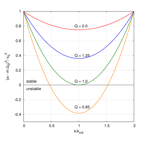
Figure 15: The normalized dispersion relation (67) for perturbations in an infinitesimally thin disk. The critical wavenumber, $k_{\rm crit}$ is given by eq. (64) and the Toomre number, $Q$ by eq. (65). For $Q=0$ marginal stability is reached. For large $k$, i.e. small wavelengths, the disk is stabilized by pressure (sound waves) and for small $k$ by a reduced density $\Sigma_{0}$. Increasing rotation $\kappa_{0}$ stabilizes as $Q$ rises.

Finally, we make the so-called tight winding approximation, which means $kr\gg m$, i.e. the radial wavelength ($1/k$) is small against the azimuthal ($r/m$). This implies that all terms containing the azimuthal wavenumber $m$ on the right hand side in eqs. (57) to (59) can be neglected. The last problem relates to the evaluation of the perturbation of the disk potential, $\tilde{\psi}_{1}$. This is obtained not from the Poisson-integral (53) but rather from the linearized Poisson-equation

$$\nabla^{2}\psi_{1}=4\pi G\Sigma_{1}\delta(z)\,,$$ (61)

where we assume a matter distribution that is only non-zero within the plane of disk ($z=0$), i.e. $\delta(z)$ denotes the $\delta$-function. Integrating eq. (61) over a small volume around the disk one obtains 2010apf..book.....A

$$\tilde{\psi}_{1}=-\frac{2\pi G\tilde{\Sigma}_{1}}{|k|}\,,$$ (62)

and eqs. (57) to (59) turn into the dispersion relation 1964ApJ...140..646L

$$(\sigma-m\Omega_{0})^{2}=\kappa_{0}^{2}+c^{2}_{\rm s_{0}}k^{2}-2\pi G|k|\Sigma_{0}\,.$$ (63)

Remembering the time dependence of the perturbations, $\propto e^{i\sigma t}$, it is clear that in general perturbations are: a) Stable, for $\sigma^{2}>0$ because in this case $\sigma$ is real and the disturbances oscillate in time with a frequency $\sigma$, or they are b) Unstable, for $\sigma^{2}<0$ because in this case $\sigma$ is imaginary and the disturbances can grow exponentially, leading to an unlimited growth, i.e. instability. The point of marginal stability is given by $\sigma=0$. From our relation (63) one can see that the epicyclic oscillations ($\kappa_{0}$ - term) are stabilizing at all spatial scales, this is the classical Rayleigh stability criterion. Indeed, for individual particles orbiting a central object that are slightly perturbed, $\kappa_{0}$ is the oscillation frequency of the particle around its equilibrium position. In the case of a spread out gas the propagation of sound waves and self-gravity come into play. For the sound waves ($c_{\rm s}$ - term) the stabilizing effect is larger for larger $k$, i.e. for smaller spatial scales. On the other hand, the last term in eq. (63) refers to the effect of the self-gravity of the disk which is always destabilizing due to the minus sign and proportional to the local surface density, $\Sigma_{0}$.

Let us now consider axisymmetric disturbances with $m=0$. Since for stability the frequencies must be real, $\sigma^{2}\geq 0$, the most unstable oscillations are those where $\sigma^{2}$ is minimal. Because $\sigma$ is a function of $k$ the most unstable critical wavelength, $k_{\rm crit}$, can be calculated from $d\sigma^{2}/dk=0$, and we obtain

$$k_{\rm crit}=\frac{\pi G\Sigma_{0}}{c_{\rm s}^{2}}\,,$$ (64)

where we drop for simplicity the index $0$ at the sound speed. Substituting this into the dispersion relation (63) and investigating the point of marginal stability by setting $\sigma^{2}(k_{\rm crit})=0$ we obtain after rearranging

$$Q\equiv\frac{c_{\rm s}\kappa_{0}}{\pi G\Sigma_{0}}=1\,,$$ (65)

where we defined the Toomre parameter $Q$. This relation implies that $Q=1$ defines the borderline between stable and unstable configurations, the marginal state. Indeed, from the dispersion equation (63) that is quadratic in $k$ one can show that in the case of axisymmetric disturbances the following inequality must be satisfied for stability 1992pavi.book.....S

$$\text{For stability:}\quad\quad Q>1\quad\quad\mbox{(Toomre-Criterion)}\,.$$ (66)

As just discussed above and directly seen from (66), for a given $\kappa_{0}\approx\Omega_{\rm K}$ the disk will be stabilized by higher temperatures (increase in $c_{\rm s}$) implying thicker disks, while a larger surface density will lead to destabilization. Hence, whenever $Q$ is of the order unity the disk is prone to instability. Using these definitions for $k_{\rm crit}$ and $Q$ the dispersion relation (63) can be rewritten as

$$\left(\frac{\omega-m\Omega_{0}}{\kappa_{0}}\right)^{2}=1+\frac{1}{Q^{2}}\,\left(\frac{k^{2}}{k_{\rm crit}^{2}}-2\frac{|k|}{k_{\rm crit}}\right)\,.$$ (67)

This function is displayed graphically in Fig. 15 for different $Q$ values. Obviously, the minima of the parabolas occur always at $k=k_{\rm min}$ and for $Q=1$ it coincides with marginal stability.

After having obtained now a useful criterion for disk instability, it remains to be seen what happens actually to an unstable disk. Before doing so, let us consider the situation in the Solar System. For the protosolar nebula at 10 AU with $H/r\approx 0.05$ (i.e. $c_{\rm s}\approx 0.33$km/s), a value $Q=1$ requires $\Sigma_{0}\simeq 10^{3}$ g/cm², which is much larger than the MMSN value ($\approx 50$ g/cm²). This implies that for the Solar System the gravitational instability could only have worked in an early evolutionary phase, when the mass of the protosolar nebula was still high. Using the critical wavelength $\lambda_{\rm crit}=2\pi/k_{\rm crit}$ the mass of such a fragment can be estimated to be around

$$M_{\rm p}\sim\pi\Sigma_{0}\lambda_{\rm crit}^{2}=\frac{4\pi c_{\rm s}^{4}}{G^{2}\Sigma_{0}}\sim 2M_{\rm Jup}\,$$ (68)

which lies in the range of the most massive gas giant in the Solar System. The idea of Solar System planet formation via gravitational instability goes back to Kuiper 1951PNAS...37....1K or Cameron 1978M&P....18....5C .

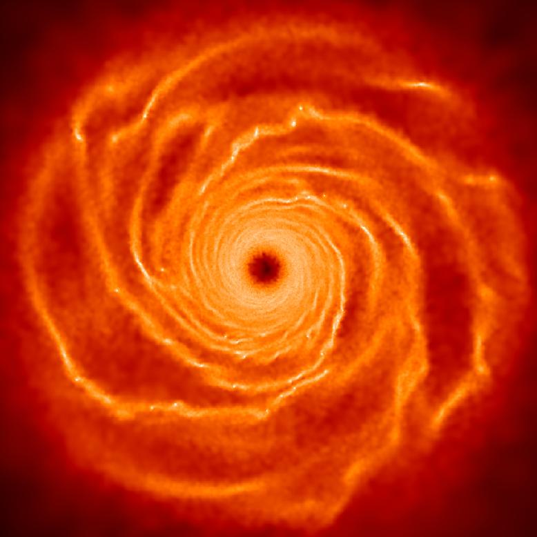
Figure 16: An example of an SPH simulation of a self-gravitating disk. During the evolution spiral arms are forming that are later fragmenting into a number of individual planet like objects. For details of the simulation see section 5.4 below. Courtesy: Farzana Meru.

5.3 Fragmentation conditions

Many non-linear hydrodynamic simulations have been performed to study the fate of unstable disks. In such simulations, typically a young protostar with a mass in the range of $(0.5-1.0)M_{\odot}$ is surrounded by a disk having a mass of a few tenth of the stellar mass. When approaching the stability limit, which is usually done by increasing the disk mass with respect to the stellar mass, the main outcome is the formation of spiral arms of low order azimuthal wavenumber, very similar to galactic disks 1998ApJ...504..945L ; 2005ApJ...619.1098M .

To determine those areas which are most susceptible to fragmentation let us consider an accretion disk with a constant mass flow through the disk, $\dot{M}=3\pi\nu\Sigma$. In an accretion disk the effective viscosity is given by

$$\nu=\alpha c_{\rm s}H=\alpha c_{\rm s}^{2}/\Omega\,,$$ (69)

and we find for the Toomre-$Q$

$$Q\propto\frac{c_{\rm s}^{3}}{\dot{M}}\,.$$ (70)

Assuming that $\dot{M}$ does not vary too strongly with radius this implies that $Q$ falls off with radius because the disks become cooler at larger distances from the star. Hence, the most unstable region lies in the outer parts of the disk. This trend is clearly seen in early 3D grid-based simulations by A. Boss 1997Sci...276.1836B where he studied the evolution of isothermal and adiabatic disks with a mass of about $140M_{\rm Jup}$ within 10 AU around a Solar mass star. In both cases clumps formed near the outer boundary. Similar results were obtained with the Smooth Particle Hydrodynamics (SPH) method. Using over one million particles in isothermal simulations is was shown that fragments of planetary mass can form easily 2002Sci...298.1756M and on very short timescales of only a few hundred years. A typical example on how such a simulation looks like is shown in Fig. 16. This strong reduction in assembly-time clearly shows the great interest in the GI-mechanism as a possible path to giant planet formation. On the other hand for adiabatic simulations it was found that the forming clumps were sheared out and dispersed 2004ApJ...609.1045M .

These results clearly indicate that the outcome, whether or not fragments are forming, will depend not only on the present value of the temperature but on the disk thermodynamics, that determines how the matter reacts upon compression. The internal temperature of the disk is determined by the balance of heating and cooling processes. If the cooling is higher than the heating, the disk will be unstable, if it is lower, the disk will be stable. For the disk we have the following heating mechanisms operating:

• internal dissipation in shock waves, for example produced by spiral arms

• effective viscosity, produced by the turbulent motion within the disk. This is typically modeled via standard viscous dissipation for example in an $\alpha$-disk model as in eq. (69)

• heating by external sources such as the central star, cosmic rays or nearby stars. This will be more important in the outer parts of the disk

On the other hand the following cooling mechanisms can be considered

• equation of state (EOS)
  The EOS determines the behavior of the gas upon compression. A medium that can be strongly compressed without heating up will be more susceptible to instability than a medium that heats up strongly. The following cases are often considered in running disk models:
  EOS1 - (locally) isothermal. Here the disk temperature is a given function of radius that cannot change. This is equivalent to strong cooling, i.e. the gas cannot heat up upon compression
  EOS2 - locally isothermal for low gas densities, then adiabatic above some suitable $\rho_{\rm crit}$. This type of EOS models the turnover from an optically thin gas of low density and a denser medium that heats up upon compression. This type frequently used in star formation simulations 2004RvMP...76..125M

• simple cooling laws
  Quite generally the cooling time is defined by

  $$t_{\rm cool}=\frac{e_{\rm th}}{de_{\rm th}/dt}\,,$$ (71)

  where $e_{\rm th}$ is the thermal energy of the disk per surface area. Simple approximations are often used in the context of planet formation
  $t_{\rm cool}\Omega=const.$   ($t_{\rm cool}$ is a fixed fraction of the local rotational period.)
  $t_{\rm cool}=const.$   ($t_{\rm cool}$ is fixed throughout)

• radiative cooling   (from disk surfaces)
  The Rosseland mean opacity is proportional to $\kappa_{\rm R}\propto Z\,T^{\epsilon}$, where the magnitude of $\kappa_{\rm R}$ is given by the amount of dust particles embedded in the disk, with the metal abundance $Z$. If one assumes that the energy is locally radiated away from the two disk surfaces with the flux, $F_{\rm eff}=\sigma_{\rm B}T_{\rm eff}$, then

  $$t_{\rm cool}\simeq\frac{e_{\rm th}}{2\sigma_{\rm B}T^{4}_{\rm eff}}\propto T/T_{\rm eff}^{4}\propto T^{-3+\epsilon}\,Z$$ (72)

  where we have assumed an optically thick case where the midplane temperature is related to the surface temperature via

  $$T^{4}_{\rm eff}=T^{4}_{\rm mid}/\tau$$ (73)

  using the mean vertical optical depth, $\tau\sim\Sigma\kappa_{\rm R}$. Typically: $-3<\epsilon<3$, such that $t_{\rm cool}$ grows with lower temperature

The last option, radiative cooling in combination with a realistic EOS is certainly the most realistic approximation one can make for flat two-dimensional disks but often the simple cooling laws are used.

As pointed out, the likelihood for fragmentation depends on the cooling timescale of the gas. For rapid cooling the system will be more likely to fragment than systems where the cooling rate is longer. Often, a simple $\beta$-cooling law is applied in numerical simulations with

$$t_{\rm cool}=\beta\,\Omega^{-1}\,,$$ (74)

and a constant value of $\beta$. In a linear analysis for the local shearing sheet it was then shown 2001ApJ...553..174G that the instability is then determined directly by the value of $\beta$, in particular

$$t_{\rm cool}\leq 3\Omega^{-1}\quad \Rightarrow$$ fragmentation (75)

$$t_{\rm cool}\geq 3\Omega^{-1}\quad \Rightarrow \quad\mbox{no fragmentation}\,.$$ (76)

This implies that $\beta_{\rm crit}=3$ is the critical value 2001ApJ...553..174G . A simple estimate for $\beta$ in accretion disks can be obtained from thermodynamic equilibrium where it is assumed that the internally produced heat is radiated away locally leading to the following cooling behaviour 1981ARA&A..19..137P

$$\frac{e_{\rm th}}{t_{\rm cool}}=\Sigma\nu\left(\frac{d\Omega}{dr}\right)^{2}\,.$$ (77)

Here, it was assumed that the heat generation, produced for example by gravo-turbulence for marginally stable self-gravitating disks, can be written as an effective viscous dissipation with kinematic viscosity $\nu$. For an ideal gas with the thermal energy $e_{\rm th}=c_{\rm v}\Sigma T$, where $c_{\rm v}$ denotes the specific heat at constant volume, an $\alpha$-viscosity as in eq. (69), and Keplerian rotation, one finds for the equilibrium state

$$\Rightarrow\quad\quad t_{\rm cool}\simeq\frac{4}{9}\frac{1}{\gamma(\gamma-1)\alpha}\,\Omega^{-1}\,.$$ (78)

As to be expected, the cooling ability of the gas directly determines the level of viscosity in the disk. locally. For $\alpha\sim 10^{-2}$ and $\gamma=1.4$ we find with $e=\Sigma c_{\rm v}T$ a cooling time of $t_{\rm cool}\sim 12$ periods. This is roughly the timescale for changes of the thermal structure of an accretion disk.

One should keep in mind however that eq. (78) describes the equilibrium situation for the disk and local variations are to be expected in realistic cases. Additionally, the simple $\beta$-cooling that went into the derivation of (78) is not a realistic cooling, as it does not depend on the density of the gas. When a gas clump is compressed it is to be expected that the cooling time rises and the clump will heat up preventing further collapse, i.e. for a realistic modeling more sophisticated cooling prescriptions, such as (72) will have to be applied. Applying the $\beta$-cooling prescription (74) simulations performed in the 2D shearing-sheet approximation using grid-based numerical models give results in rough agreement with the above fragmentation condition 2001ApJ...553..174G , as do corresponding global 3D disk models using the SPH method 2003MNRAS.339.1025R . However, using very high resolution simulation in the 2D isothermal setup, it was shown that even for $\beta\approx 20$ fragments could form due to the stochastic nature of the turbulent flow 2012MNRAS.421.3286P .

As just mentioned, for fragmentation to occur in disks a cooling time shorter than $\approx 3\Omega^{-1}$ is required. From the definition of $Q$ (65), using representative disk conditions with $H/r=0.05$, one can obtain estimates on the cooling time. Assuming a disk close to possible instability by setting $Q=1.5$, and using eq. (73) for the optical depth one finds the following relation for the cooling time 2010apf..book.....A

$$t_{\rm cool}\Omega\sim 10\,\tau\,\left(\frac{r}{5AU}\right)^{-1/2}\,.$$ (79)

Noticing that in optically thick disks the optical depth can easily reach $10^{2}$ and more, this last relation seems to imply that there is no possibility for fragmentation at typical planet formation locations in the Solar System. This finding represents the fact that the fragmentation requirement, high mass (implying large $\Sigma$ and high $\tau$) and low cooling times (low $\tau$) contradict each other. The presented arguments are based on the assumption of vertical energy transport by radiation (relation 73). Including vertical convective energy transport the disk can cool faster and the situation improves somewhat. For lower temperatures the opacities are lower and the cooling time is reduced again. Including additionally external perturbation, for example by a passing star that compresses the outer regions in the disk, a gravitational instability may be triggered. In summary one may conclude that, if at all, fragmentation can only be expected at very large radii from the star beyond 50 AU or so 2005ApJ...621L..69R .

5.4 Non-linear simulations

At the end of this section we would like to summarize briefly the results of a few recent numerical simulations concerning the fate of gravitational unstable disks. This is not an exhaustive review as there have been many simulations concerning this topic and the issue is not conclusively decided at present. A summary of the field was given in the Protostars and Planets V proceedings 2007prpl.conf..607D where different numerical methods were directly compared using similar initial initial conditions. The codes used in the comparison included particle methods such as SPH (the public codes GASOLINE and GADGET) as well as the grid codes that used finite difference or finite volume methods either based on upwind schemes (Indiana Code) or Riemann-solvers (FLASH). It was noted that the outcome of the simulations depends crucially on numerical aspects such as spatial resolution (number of grid-points, or particles), regularization methods (smoothing length, artificial viscosity, flux-limiters), solver for self-gravity (smoothing criteria) and so on. Hence, it was concluded that in order to obtain reliable results it seems unavoidable to compare different methods on the same physical problem. Using appropriate criteria for the individual codes similar results could be obtained. One should keep in mind however, that the results obtained with different codes on this problem will never be identical because of the chaotic nature of the problem. Hence, the results can only be compared in a statistical sense.

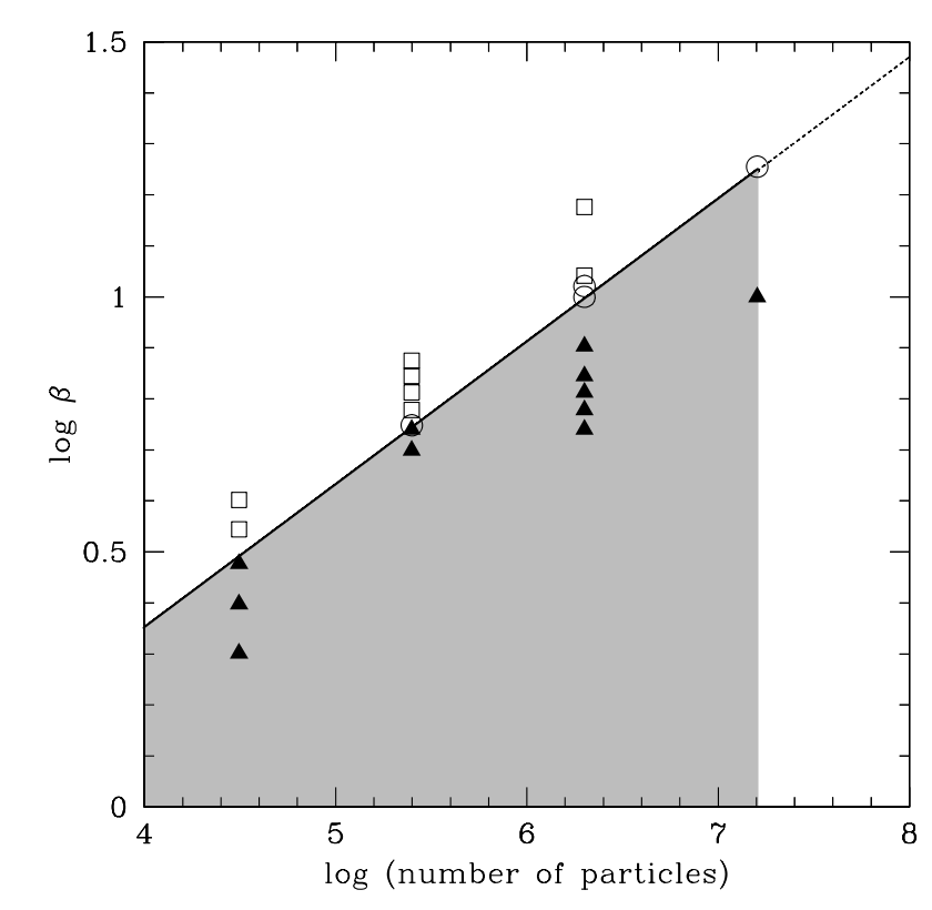
Figure 17: The cooling rate $\beta$ against numerical resolution (here the used particle number) for SPH-simulations of self-gravitating disks, here a $0.1M_{\odot}$ disk around a one solar mass star. The symbols denote the numerical outcome: non-fragmenting (open squares), fragmenting (solid triangles) and borderline (open circles) simulations. The borderline simulations are those that initially fragment but whose fragments are sheared apart. The solid black line separates fragmenting and non-fragmenting cases and the gray region marks the fragmentation regime. Taken from 2011MNRAS.411L...1M

The convergence issue

The sample study of Meru & Bate 2011MNRAS.411L...1M illustrates one of main numerical problems very well. They considered the situation of a $0.1M_{\odot}$ disk around a $1M_{\odot}$ star spanning a factor of ten in radii, ranging from $0.25$ to $25$ (in dimensionless units). For the cooling they used the $\beta$-prescription (74) with different values for $\beta$ within $2.0\leq\beta\leq 18$. They performed SPH-simulations using a huge range of different particle numbers from $N=31,250$ to $N=16$ million particles. A typical result of such a simulation is displayed in Fig. 16. The results indicate that the value of $\beta$ below which fragmentation occurs depends strongly on the particle number used in the simulations. As shown in Fig. 17 the critical value of $\beta$ increases monotonically with $N$ as given by the solid line. The hatched region indicated the fragmentation regime while above the line the disks are stable. Clearly, there is no real indication of convergence in these simulations. Because the aforementioned SPH simulations are fully three-dimensional and hence require a very high particle number for numerical convergence, an alternative option that has been used frequently is the two-dimensional grid code FARGO 2000A&AS..141..165M that has been empowered with a self-gravity module in 2D 2008ApJ...678..483B . Comparing both codes, SPH and FARGO, Meru & Bate 2012MNRAS.427.2022M find that the question of convergence hinges at the treatment of numerical viscosity, for both codes. They argue that convergence can be reached yielding critical $\beta$-values of about 20 to 30, making fragmentation easier. A detailed analyses and additional SPH simulations using an improved cooling prescription as well improved artificial viscosity (and consequently artificial dissipation) found numerical convergence and fragmentation occurring for cooling times between $\beta=6$ and $\beta=8$ for an adiabatic index $\gamma=5/3$ 2014MNRAS.438.1593R . They also find that fragmentation can occur only at very large distances beyond at least 50 AU, in agreement with the above expectations 2005ApJ...621L..69R , and as seen in other studies 2010ApJ...710.1375K ; 2013A&A...552A.129V . These cases demonstrate again the numerical problems that are still present in such self-gravitating disk simulations, and indicate the necessity to compare different codes and methods.

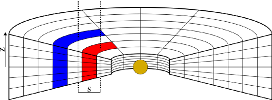
Figure 18: Geometry of a protoplanetary disk around a central star to illustrate the requirements for the calculation of the disk’s self-gravity in 2D simulations. The goal is to calculate the gravitational force exerted by a vertical slice of the disk (blue) on another vertical slice of the disk (red), that are separated by the projected distance $s$. As seen in the drawing, two vertical integrations have to be performed along the dashed lines that go through the cell centers assuming cylindrical coordinates. To obtain the total force between the two segments, this value has to be multiplied by the corresponding areas, see also Eq. (5.4). Taken from 2012A&A...541A.123M

The gravitational potential

Care has to be taken when treating the disk in a flat 2D geometry only. Even though the disk may be vertically thin, the gravitational potential has to be modified to account correctly for the vertical extent of the disk 2012A&A...541A.123M as illustrated in Fig. 18. The potential at a point $\vec{r}$ generated by the remaining part of a self-gravitating disk is given by

$$\Psi_{\mathrm{sg}}(\vec{r})=-\int_{\rm Disk}\frac{G\rho(\vec{r}^{\prime})}{\left|\vec{r}-\vec{r}^{\prime}\right|}\,d\vec{r}^{\prime}\,.$$ (80)

Here, in contrast to the earlier expression (53) the full vertical stratification of the disk has been taken into account. As the standard 2D hydrodynamic equations (49) to (51) are obtained by an averaging process over the vertical direction, this has to be done for the gravitational potential as well. This is typically approximated by a suitably chosen smoothing parameter. For this purpose it is convenient to analyze the force between to individual elements (segments) of the disk. The potential at the location $\vec{r}$ generated by a disk element located at $\vec{r}^{\prime}$ which is a projected distance $s$ away is given by

$$\Psi_{\mathrm{sg}}(\vec{r})=-\iiint\frac{G\rho(r^{\prime},\varphi^{\prime},z^{\prime})}{\left(s^{2}+(z-z^{\prime})^{2}\right)^{\frac{1}{2}}}\,dz^{\prime}\,dA^{\prime}\,.$$ (81)

Here $dA^{\prime}$ is the surface element of the disk in the disk’s midplane (the $z=0$ plane) that is located at the point $\vec{r}^{\prime}$, separated by the projected distance $s$. The force at the position $\vec{r}$ due to the rest of disk is calculated from the gradient of the potential (81), and vertical averaging leads to the following force density 2012A&A...541A.123M

$$F_{\mathrm{sg}}(s) =-\int\rho(r,\varphi,z)\frac{\partial\Psi_{\mathrm{sg}}}{\partial s}\,dz$$

$$=-Gs\iiiint\frac{\rho(r^{\prime},\varphi^{\prime},z^{\prime})\,\rho(r,\varphi,z)}{\left(s^{2}+(z-z^{\prime})^{2}\right)^{\frac{3}{2}}}\,dz^{\prime}\,dA^{\prime}\,dz\,,$$ (82)

where the integral is over the vertical extent (at position $\vec{r}$) and all other locations of the disk. Even under the assumption that the vertical structure of the disk is given analytically (e.g. a simple Gaussian), the computation of the force (5.4) is extremely costly. Hence, the potential (81) is approximated often by the so-called $\epsilon$-potential

$$\Psi^{\mathrm{2D}}_{\mathrm{sg}}(s)=-\iint\frac{G\Sigma(\vec{r}^{\prime})}{\left(s^{2}+\epsilon_{\mathrm{sg}}^{2}\right)^{\frac{1}{2}}}\,dA^{\prime}\,,$$ (83)

where $\epsilon_{\mathrm{sg}}$ is the smoothing length for self-gravitating disks that takes into account the unresolved vertical extend of the disk. The force acting on each disk element is then calculated from the gradient of $\Psi^{\mathrm{2D}}_{\mathrm{sg}}$. This formulation extends eq. (53) for numerical simulations and the smoothing length does not only ensure that the numerical evaluation remains finite but is physically necessary due to the finite disk thickness. By comparing the results obtained with (83) to the exact formulation (81) (using a Gaussian vertical density profile) one obtains a good match with $\epsilon_{\rm sg}\approx H$ 2012A&A...541A.123M .

Fragmentation outcome and longterm evolution

As a massive protoplanetary disk may still be embedded somewhat in their envelope it is important to model the disk evolution in combination with infall onto the disk. Such studies have been performed through 2D numerical simulations of viscous disks that include radiative cooling, stellar irradiation, and mass infall 2012ApJ...746..110Z . The results show that fragmentation is possible when mass infall is included. However, two major problems have been identified:   a) Mass challenge: To be able to fragment the disk must have a high mass ($M_{\rm disk}>0.3M_{\odot}$) and requires a high infall rate. The fragments then grow very fast and typically end up as Brown Dwarfs (BD) with masses well above the planetary regime.   b) Migration challenge: Once formed the fragments migrate inward rapidly on a timescale $<1000$yrs. Only large masses survive, and small ones get tidally disrupted. The authors conclude that that GI will lead to massive BDs or binaries. The migration problem will be discussed also in the following section. Similar findings have also been found in full 3D simulations of fragmenting disks 2013MNRAS.436.1667T .

Important further aspects concern the subsequent evolution of the clumps after they have formed. As just mentioned they migrate inward very rapidly and can be tidally disrupted upon reaching the inner region of the accretion disk close to the central star. This can lead to accretion events such as FU Ori outbursts that occur in the early phase of star formation when the disk is still very massive 2006ApJ...650..956V . As an alternative, the tidal downsizing scenario considers another fate of the clumps. Upon inward migration the Roche radius of the massive clumps is shrinking continuously such that they might lose their envelopes by tidal effects through mass overflow across the $L_{1}$ Lagrange point, see Fig. 7. The final outcome could be objects with much smaller mass, sometimes even rocky planets 2010MNRAS.408L..36N . In this scenario the above mentioned mass challenge would be resolved as the clumps loose the majority of their mass, and the gas giants could be assembled on a short timescale.

After having discussed two different pathways (by CA or GI) in forming giant planets, it is interesting to ask if one can possibly distinguish them. The answer lies in the thermal evolution of the young planets. Planets formed by gravitational instability are thought to have higher entropy, larger radii, and possibly higher effective temperatures than core-accretion objects, because of the stored heat in the accumulated gas that did not have time to cool during the rapid accretion process. Following the longterm thermal evolution it has been shown that for planets with mass less than about 5 $M_{\rm Jup}$ differences in the effective temperature persist for a few million years only, while for planets of higher mass it can take up to about 100 million years before equilibration 2012ApJ...745..174S . However, the feasibility of this distinction hinges on details of the models. For example, the accretion of additional solid material during the subsequent evolution will enhance the cooling of the planets formed by GI and reduce the differences to the CA planets, implying that it might be difficult to separate the two options observationally.

As a final remark, concerning possible difficulty of producing gaseous planets directly through the GI process we would like to point out that even the formation of planetesimals may be enhanced in the early phases of very massive disks. As shown in the previous section, small bodies experience gas drag and will drift towards pressure maxima occurring in the disk. As it turns out, in marginally stable disks the spiral arms may be sufficiently long lived to support the collection of particles in them such that the concentrated dust particles can collapse to their own self-gravity to form directly planetesimals in the early phase of planet formation 2006MNRAS.372L...9R .

Forming planets by direct gravitational instability of the disk has long been considered as an alternative option to the core instability pathway. An advantage would be the associated short time scale of the formation process. As stated by the well-known Toomre criterion, for the mechanism to work the disk must be sufficiently massive and and at low temperature. In order for the collapse to proceed the gas must be able to cool sufficiently fast to get rid of the thermal energy. The required cooling times are only a few (3-5) dynamical timescales. These conditions, high disk mass and short cooling times can only be fulfilled in the very outer parts of a protoplanetary disk, probably only beyond a distance of about 50 AU. Hence, it represents a possible formation scenario for the distant planets detected by the direct imaging method.

6 Planet-disk interaction

In the preceding section we have implicitly assumed that the planets remain on their orbits during the growth phase. This in-situ formation process is based on the situation in the Solar System in which the large planets reside further out where they could accrete large amounts of gas, while the terrestrial planets are located further in where, due to the higher disk temperatures, only small amounts of gas were available to be accreted onto the rocky cores. Comparing this situation with the observed semi-major axis distribution of the extrasolar planets (as shown in Fig. 2) it was clear from the very beginning, in fact already after the discovery of the very first object, 51 Peg, by Mayor & Queloz 1995Natur.378..355M , that the presence of close-in planets is difficult to explain by an in-situ formation process. This is because close to the star the amount of solids available for core formation is not sufficient and the disk temperature is too high to condense the gas. For an alternative point of view see for example 2000Icar..143....2B . This difficulty led to the immediate suggestion that 51 Peg had formed in the standard way at larger distances, similar to Jupiter in the Solar System, and subsequently drifted inward driven by planet-disk interaction 1996Natur.380..606L . Such a migration process is a natural consequence of the planet formation process because the gravitational interactions between the planet and the ambient disk will necessarily lead to forces acting on the planet causing it to change its orbital elements. In this section we will describe the physical processes of disk-planet interaction in more detail. Recent reviews of the topic are presented in the Protostars and Planets (V and VI) proceedings 2007prpl.conf..655P ; 2014prpl.conf..667B or in 2013LNP...861..201B and 2012ARA&A..50..211K .

6.1 Basic concepts

Embedding a planet into the disk leads to characteristic disturbances in the density of the disk. Due to the shearing motion in the disk the sound waves emanating from the planet’s location are sheared out and spiral waves are forming. As shown in Fig 19 on the left panel, the inner spiral is leading and the outer one trailing, where the planet moves counterclockwise around the star.

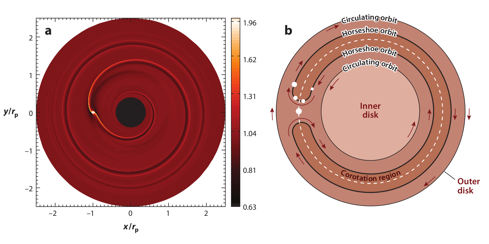
Figure 19: The influence of a planet that is embedded in a protoplanetary disk. The planet moves counterclockwise around the central star which is located in the center of the two plots. The left panel (a) shows the surface density distribution (in dimensionless units) of a 10 $M_{\rm Earth}$ planet on a circular orbit that is embedded in a disk of constant density. Shown is the configuration at about 20 orbits after insertion of the planet. The planet is a unit distance away from the star at the location $x=-1,y=0$. The right panel (b) shows a schematic plot of the motion of gas particles (smaller white dots) on orbits close to the planet. The motion is depicted using red arrows in a reference frame corotating with the planet. The horseshoe region that is corotating with the planet is shown in the dark brown color, while the inner and outer circulating orbits are shown in the lighter color. Taken from Kley & Nelson 2012ARA&A..50..211K

These spiral waves represent over densities in the gas distribution and generate a net force acting on the planet that changes its orbit. The second contribution to the forces comes from the corotation region of the planet which is depicted in the right panel of Fig. 19. For single particle trajectories the dynamics on both sides of the planet would be identical. However, for fluid motion there exists a small asymmetry between the U-turns of the gas in front and behind of the planet which generates again a net force on the planet. For a planet of mass $m_{\rm p}$ on a circular orbit its angular momentum is given by

$$J_{\rm p}=m_{\rm p}r_{\rm p}^{2}\Omega_{\rm p}\,,$$ (84)

where $r_{\rm p}$ is the distance of the planet from the star and $\Omega_{\rm p}$ its orbital speed. The density asymmetries generate a torque, $\Gamma_{\rm p}$, acting on the planet that changes the angular momentum according to

$$\dot{J}_{\rm p}=\Gamma_{\rm p}\,.$$ (85)

Here, $\Gamma_{\rm p}$ denotes the $z$-component of the total torque that needs to be calculated adding the individual contributions of the whole disk

$$\Gamma_{\rm p}=-\int_{\rm disk}\Sigma(\vec{r}_{\rm p}\times\vec{F})\,df\,=\,\,\int_{\rm disk}\Sigma(\vec{r}_{\rm p}\times\nabla\psi_{\rm p})\,df\,=\,\,\int_{\rm disk}\Sigma\frac{\partial\psi_{\rm p}}{\partial\varphi}df\,.$$ (86)

In eq. (86) we assume a flat two-dimensional disk, where $\vec{F}$ denotes the gravitational force per unit mass between the planet (located at $\vec{r}_{\rm p}$) and a small surface element, $df$, of the disk which has the surface density, $\Sigma(r,\varphi)$. $\psi_{\rm p}$ denotes the gravitational potential of the planet. From eq. (86) we can infer that it is exactly the asymmetry in the azimuthal direction that changes the angular momentum of the planet. From eqs. (84, 85) and using Keplerian rotation

$$\Omega_{\rm K}(r)=\sqrt{\frac{GM_{*}}{r^{3}}}\,,$$ (87)

we can calculate the change in the planet’s distance as

$$\frac{1}{r_{\rm P}}\,\frac{dr_{\rm P}}{dt}\,\equiv\,\frac{1}{\tau_{\rm M}}\ =\,2\,\frac{\Gamma_{\rm p}}{J_{\rm P}}\,,$$ (88)

where we introduced the migration timescale $\tau_{\rm M}$. To infer the importance of the planetary migration, this timescale needs to be compared to the overall evolution time of disk.

Obviously, the analysis of the migration process comes down to the calculation of the torques acting on a planet. As we shall see below in Sect. 6.5 this statement refers to planets on circular orbits only, otherwise the power acting on the planet has to be considered as well. In principle, according to eq. (86), this appears to be an easy evaluation. The problem lies in the fact that the total torque is always the difference between a positive and negative contribution that have nearly the same magnitude. As a consequence the total torque depends delicately on physical aspects of the disk such as viscosity, or heat diffusion. As we shall see, this does not only influence the speed of the migration but can change even the overall direction.

The calculation of the total torque can be performed by different approaches. For lower mass planets that perturb the density of the disk only mildly one can perform a linearization of the hydrodynamic equations around the unperturbed disk without the planet, similar to the methods shown in the previous section. Here, the basic state is given by an axisymmetric disk that is in pure rotation around the star with $\Omega(r)$ and has a given $\Sigma(r)$ profile and possibly temperature gradients. The planet is then added as a small disturbance via an additional potential that rotates with the speed $\Omega_{\rm p}$. Linearizing the equations yields a new perturbed disk structure, whose back reaction on the planets gives the torque, and hence the migration rate. In the azimuthal direction the potential can be expanded in a Fourier-series due to the periodicity. Using this procedure, the strongest perturbations in the disk are excited at particular resonances where the pattern speed of individual Fourier-components of the perturbed potential, $\omega=m(\Omega(r)-\Omega_{\rm p})$, matches a natural frequency of oscillation in the disk. The first resonance is the corotation resonance that occurs for material at the location of the planet which has $\Omega=\Omega_{\rm p}$. These are related closely to the horse-shoe drag that we will discuss below. Other resonances are excited at the those locations where the pattern speed $\omega$ matches the epicyclic frequency $\kappa$, see eq. 60. These are the Lindblad resonances that may occur inside of the planetary orbit or outside.

In the second approach the torques are obtained from full non-linear hydrodynamic simulations of embedded planets in disks. Here, the disk is initialized with an equilibrium profile of density and temperature and then the planet is added as a perturbing object to the flow. In one type of models the initial planetary orbit is fixed in time and only the disk structure changes due to the action of the embedded planet. The simulations are then evolved in time until the system has reached a quasistationary equilibrium. The torque on the fixed planet is continuously monitored and the theoretical migration speed can be calculated by eq. (88). In other models the planet is allowed to change its orbital elements according to the forces acting on it, and the change in orbital elements is directly calculated. Will not go into details of these methods but just quote the main results

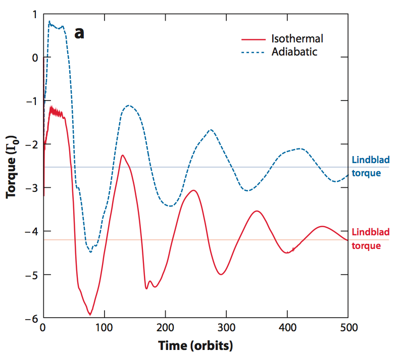
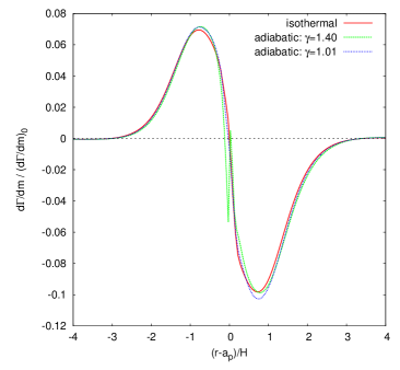
Figure 20: The torque acting on a low-mass planet on a fixed circular orbit that is embedded in a disk that has a constant surface density and very low viscosity. Shown are results from 2D hydrodynamic simulations for an adiabatic and a locally isothermal disk. The left panel shows the time evolution of the total torque acting on planet. At the start of the simulations, when the gas performs its first U-turn near the planet, the torques reach a maximum (fully unsaturated values). Then they drop to reach the final saturated values through a series of oscillations. The horizontal lines refer to the 2D isothermal and adiabatic Lindblad torques 2010MNRAS.401.1950P . The right panel shows the radial torque density in the final state, again for an isothermal and two adiabatic simulations for $\gamma=1.01$ and $\gamma=1.4$ (adapted from 2012A&A...546A..99K ). The units $\Gamma_{0}$ and $(d\Gamma/dm)_{0}$ are stated in the main text, see eqs. (90) and (94).

6.2 Type I migration

In this section we deal with lower mass planets, up to about a few Earth masses that do not perturb the disk structure significantly. In particular, these planets do not open gaps in the disk. The torques can be then analysed through linear, as well as non-linear approaches. This migration regime where the disk is only weakly disturbed is termed type I migration. In this case both contributions are important, spiral arms (Lindblad torques) as well as the corotation region.

As seen from the left panel in Fig. 19 the spiral arms are the most prominent features visible in the perturbed density distribution in disk as generated by the planet. Clearly, from a purely mechanical point of view, and loosely speaking, the inner spiral arm pulls the planet forward which leads to an acceleration of the planet and a gain of angular momentum. On the other hand, the outer spiral pulls the planet back which leads to a loss in angular momentum. This feature is reflected in the mass weighted radial torque density distribution that is displayed in the right panel of Fig. 20. The part inside of the planet is positive while the part outside is negative. The total torque is given by the integral over this distribution

$$\Gamma_{\rm tot}=2\pi\int\frac{d\Gamma}{dm}(r)\,\Sigma(r)\,rdr$$ (89)

and, as already hinted above, it is a balance between positive inner and negative outer torques. The torque density, $d\Gamma(r)/dm$, scales with the planet to star mass ratio squared and as $(H/r)^{-4}$, and we rescale our results in units of

$$\left(\frac{d\Gamma}{dm}\right)_{0}=\Omega_{\rm p}^{2}\,r_{\rm p}^{2}\,\left(\frac{m_{\rm p}}{M_{*}}\right)^{2}\,\left(\frac{H}{r_{\rm p}}\right)^{-4},$$ (90)

where quantities with index $p$ are evaluated at the planet’s position, e.g. $\Omega_{\rm p}=\Omega(r_{\rm p})$. We note that in evaluating the pressure scale height one has to choose either the isothermal or adiabatic sound speed such that $H_{\rm adi}=\sqrt{\gamma}H_{\rm iso}$. Using this scaling the torque densities for all simulations, isothermal and adiabatic, are identical (right panel in Fig. 20).

From a wave point of view the spiral arms can be treated as the superposition of the sounds waves emanating from the planet. The torques generated can then be analyzed by the mentioned linearization procedure which leads to the Lindblad resonances where $m(\Omega(r)-\Omega_{\rm p})=\pm\kappa(r)$, with the epicyclic frequency $\kappa$. The plus sign, i.e., $\Omega(r)=\Omega_{\rm p}+\kappa(r)/m$, refers to inner Lindblad resonances (interior to $r_{\rm p}$) where the disk rotates faster than the planet. The minus sign refers to the outer Lindblad resonances, i.e., $\Omega(r)=\Omega_{\rm p}-\kappa(r)/m$ (exterior to $r_{\rm p}$ and the corotation region in Fig. 19). For a Keplerian disk the epicyclic frequency matches exactly the Keplerian speed, i.e. $\kappa=\Omega_{\rm K}$ (87), and the locations of the Lindblad resonances are given by

$$r_{\rm L}=\left(\frac{m}{m\pm 1}\right)^{2/3}\,r_{\rm p}\,.$$ (91)

These resonances are named after Bertil Lindblad, who studied the dynamics of galaxies. In case of a radial pressure gradient in the disk the rotation rate is not exactly Keplerian and the resonances are shifted slightly such as to avoid a divergence at the planetary radius for large $m$ 1980ApJ...241..425G ; 1993ApJ...419..155A . This causes the torque density to peak at a certain distance, typically a pressure scale length, $H$, away from the planet, as shown in the right panel of Fig. 19.

Detailed results for the Lindblad and corotation torques in locally isothermal disks with a fixed $T(r)$ stratification have been obtained for lower mass planets, of a few $M_{\oplus}$, through full 3D analyses. These were obtained either analytically by linear analysis 2002ApJ...565.1257T or through fully non-linear simulations 2010ApJ...724..730D . The results for the total torque can be summarized as 2010ApJ...724..730D

$$\Gamma_{\rm tot}=-(1.36+0.62\beta_{\Sigma}+0.43\beta_{\rm T})\,\Gamma_{0}\,,$$ (92)

where $\beta_{\Sigma}$ and $\beta_{\rm T}$ denote the gradients of the density and temperature in the disk that are defined through the following power laws

$$\Sigma(r)=\Sigma_{0}\,r^{-\beta_{\Sigma}}\quad\quad\mbox{and}\quad\quad T(r)=T_{0}\,r^{-\beta_{\rm T}}\,.$$ (93)

The fit formula (92) has been obtained from 3D local isothermal simulations with varying gradients in $\Sigma$ and $T$, and for a viscosity of $\alpha=0.004$ 2010ApJ...724..730D . For the definition of the $\alpha$-viscosity see eq. (69). The torque normalization is given by

$$\Gamma_{0}=\left(\frac{m_{\rm p}}{M_{*}}\right)^{2}\,\left(\frac{H}{r_{\rm p}}\right)^{-2}\,\left(\Sigma_{\rm p}r_{\rm p}^{2}\right)\,r_{\rm p}^{2}\Omega_{\rm p}^{2}\,,$$ (94)

which reflects the scaling of the torque with the physical properties of the disk. Here, $\Sigma_{\rm p}$ denotes the unperturbed surface density at the location of the planet. As seen, the torque scales with square of the planet mass, $m_{\rm p}$. This is due to the fact that the perturbations in the disk induced by the planet scale directly with $m_{\rm p}$, and the back reaction on the planets adds the second factor. The opening angle of the spiral arms is given by the temperature in the disk, here through the scale height, $T\propto H^{2}$. Lower temperatures lead to tighter spirals and consequently larger torques because the torque maxima are closer to the planet (see Fig. 20). The direct scaling with the disk’s density follows immediately from the definition of the torque in eq. (86). The migration rate follows then from eq. (88). The torque formula, eq. (92) shows that for the typical gradients in the disk ($\beta_{\Sigma}$ and $\beta_{\rm T}$ larger than zero) the migration will be directed inwards. While this is encouraging in explaining the close-in observed exoplanets, the short timescale of the migration causes problems, however. Using the slope values for the minimum mass solar nebula (MMSN), $\beta_{\Sigma}=1.5$ and $\beta_{\rm T}=0.5$, we obtain $\Gamma_{\rm tot}=2.5\Gamma_{0}$ and then from Eqs. (84), (88) and (92) we find for the migration time

$$\tau_{\rm mig}\approx\frac{1}{5}\,\left(\frac{m_{\rm p}}{M_{*}}\right)^{-1}\left(\frac{m_{\rm d}}{M_{*}}\right)^{-1}\,\left(\frac{H}{r_{\rm p}}\right)^{2}\,\Omega_{\rm p}^{-1}\,,$$ (95)

where we used $m_{\rm d}=\Sigma_{\rm p}r_{\rm p}^{2}$ as a proxy for the disk mass. Looking at the speed of migration we find for a $1M_{\rm Earth}$ planet at 5 AU a migration timescale of a few $10^{5}$ yrs. This is shorter than typical lifetimes of protoplanetary disks, and this is a general result for type I migration in locally isothermal disks. Consequently, to prevent this too rapid inward radial drift, during the past years much effort has been put into finding mechanisms to slow it down.

The key to the solution lies in the corotation, or horseshoe region. Looking at the left panel of Fig. 20 one notices that directly after insertion of the planet the torques acting on the planet are much smaller than in the final equilibrium case. This is true for the isothermal, as well as the adiabatic model. In the latter, the torques are even reversed (positive) initially which would imply an outward migration. This torque reduction or reversal is caused by the flow dynamics in the corotation region. Directly after the insertion of the planet the flow begins to perform U-turns in the vicinity of the planet. As indicated in Fig. 19 by the white dots, material from the inside moves outwards and by doing so has to gain a certain amount of angular momentum from the planet. On the other side the process is reversed and the material gives angular momentum to the planet. Clearly, if there is an asymmetry in the U-turn motion in front and behind the planet there will be a net transfer of angular momentum to the planet. Because in this U-turn motion only material within the horseshoe region is involved, the asymmetry is driven by radial gradients of particular disk properties across the horseshoe region, and the resulting torque is called the horseshoe drag 1991LPI....22.1463W . The oscillatory settling of the torque is due to the motion of the material along their horseshoe orbits. The oscillation period is given approximately by the libration time of matter in the horseshoe because after each libration period the matter reaches again the planet and receives a new kick. It is the mixing of the matter in the horseshoe region that tends to wipe out the initial gradients of the flow, and eventually the corotation torques saturate 1991LPI....22.1463W . From linear analyses 1979ApJ...233..857G , it is known that the corotation torque is proportional to the radial gradient in the specific vorticity (sometimes also called vortensity)

$$\tilde{\omega}\,=\,\frac{\omega_{z}}{\Sigma}\,=\,\frac{(\nabla\times\vec{u})|_{z}}{\Sigma}\,,$$ (96)

and proportional to the radial gradient in the entropy, $S$, see 2008ApJ...672.1054B ; 2008A&A...485..877P . The quantity $\omega_{z}$ in eq. (96) is the $z$-component of the vorticity of the disk flow. For inviscid and barotropic ($p=p(\rho)$) flows one can show that $\tilde{\omega}$ and $S$ are constant along streamlines, i.e.

$$\frac{d}{dt}\left(\frac{\omega_{z}}{\Sigma}\right)=0\quad\mbox{and}\quad\frac{dS}{dt}=0\,.$$ (97)

As a consequence any initial gradients (in $S$ and $\tilde{\omega}$) are wiped out in the corotation region in the course of the simulations and the horseshoe drag vanishes 2001MNRAS.326..833B and only the (negative) Lindblad torques remain, exactly as seen in the nearly inviscid simulation presented in Fig. 20, see also 2002A&A...387..605M . Hence, the necessary physical mechanisms to maintain those gradients are viscosity and radiative diffusion, or radiative cooling 2008ApJ...672.1054B ; 2008A&A...485..877P .

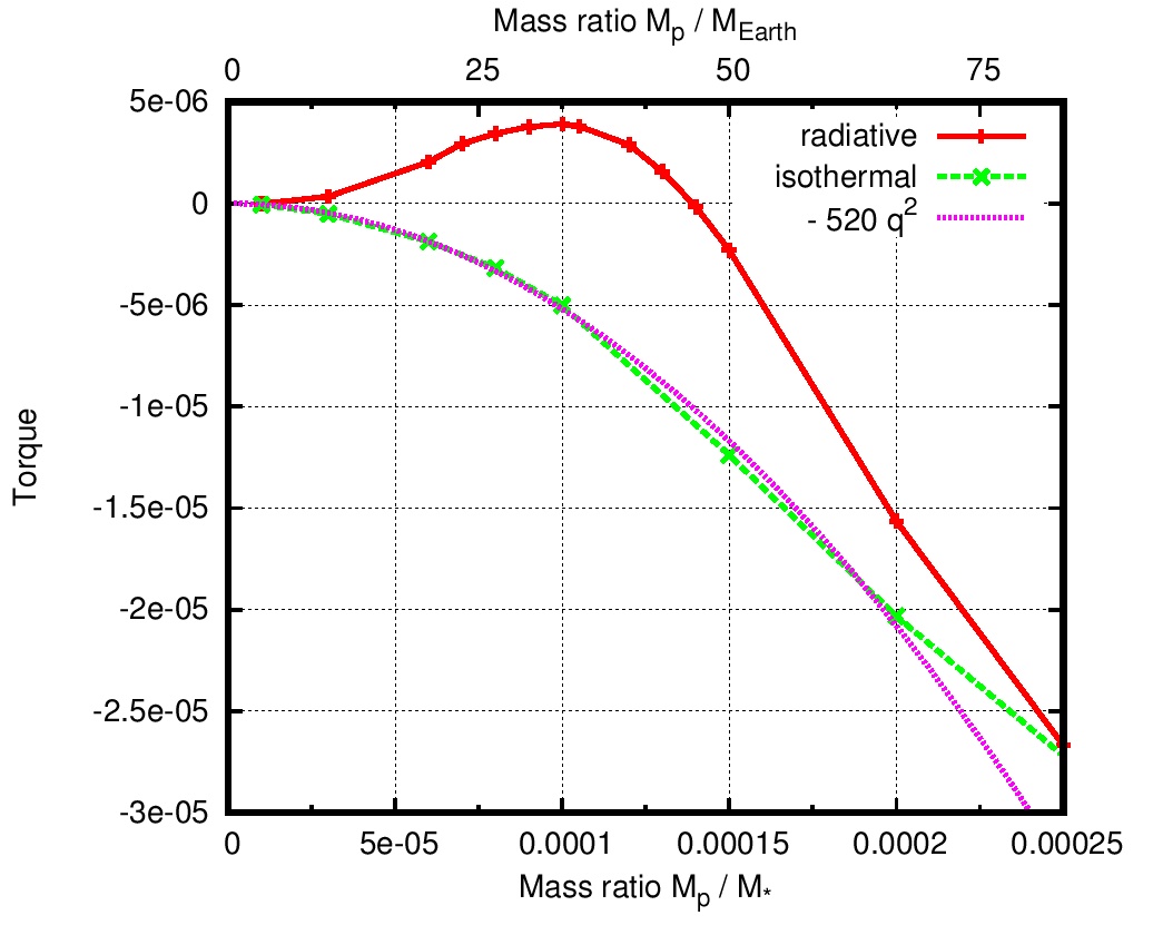
Figure 21: The torque acting on embedded planets in 2D, viscous disks using $\alpha=0.004$. Results are shown for a locally isothermal disk (green) and radiative models (red) that include viscous heating, radiative transport in the midplane, as well as radiative cooling from the disk surfaces. The purple line shows a parabola that scales with the square of the planet mass. Adapted from 2008A&A...487L...9K .

Indeed, through a series of 2D and 3D hydrodynamical simulations it has been shown in more realistic disks models which include radiative transport that the migration of planets can be slowed down and even directed outwards, see Paardekooper & Mellema 2006A&A...459L..17P for the very first simulation of this kind. Subsequently, model sequences using varying planet masses in 2D 2008A&A...487L...9K and 3D 2009A&A...506..971K for active, viscous disks with radiative transport have shown that there exists is a typical mass range in which the total torque is positive and the migration can be directed outwards. For maximum efficiency of the torque desaturation the viscous and radiative diffusion timescales should lie within the libration and U-turn timescales of the gas in the horseshoe region. Hence, it depends on the mass of the planet, and disk properties such as viscosity and opacity. An example of such a study for the 2D case with embedded planets located at 5 AU is shown in Fig. 21. For this disk regime the mass range with the fastest outward migration lies between 25 and 40 $M_{\rm Earth}$. To study the overall evolution of planets in disks it is useful to apply formulae that provide reliable estimates of the torque and can be computed fast and easily. These were provided in 2010ApJ...723.1393M ; 2011MNRAS.410..293P and confirmed by full 3D radiative simulations 2011A&A...536A..77B . The torque formulae indicate that for small planets of a few Earth masses the migration should be directed inward, a feature hardly visible in Fig. 21. Indeed, the inward migration of planets below a mass of about 3 $M_{\rm Earth}$ has been verified in 3D high resolution simulations 2014MNRAS.440..683L . Very recently, the migration of low mass planets in this mass range has been addressed by including the effect of accretional heating from the (solid) material added to the planet in the simulations. Taking this additional heat source into account, it has been found that the migration can be directed outwards for very low mass planets 2015Natur.520...63B . This heating torque effect might play an important role in preventing the too rapid inward migration of planetary cores towards their host stars. These studies indicate that the migration direction and rate of an embedded planet depends on the details of the disk flow in the close vicinity of the planet. This requires more high resolution simulations similar to the nested-grid simulations presented in 2003ApJ...586..540D , or the more recent example by 2015ApJ...811..101F .

As mentioned above, the torques acting on a planet depend on the physical disk properties (viscosity and opacity). During the evolution of the disk these will change in space and time. To account for this, sequences of 2D axisymmetric disk models that include radiative cooling and viscous and stellar heating have been computed for different evolutionary states of the host star 2015A&A...575A..28B as a function of the disk’s metallicity, accretion rate, and lifetime. The parameterized disk structures in conjunction with the torque formulae 2011MNRAS.410..293P form an ideal setup for studying the longterm evolution of planets in disks.

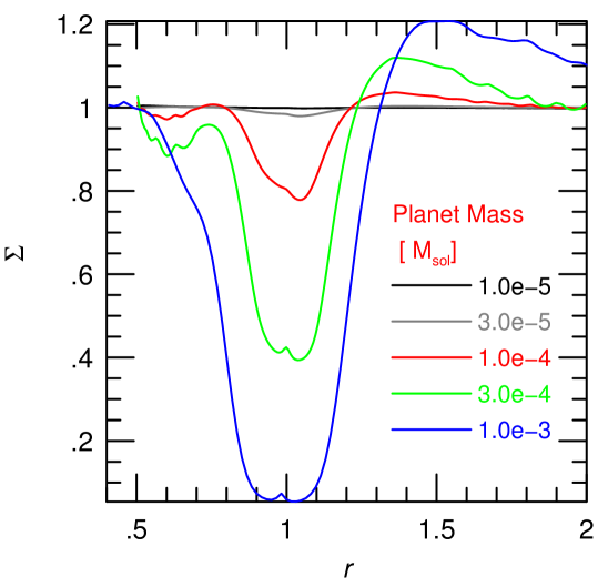
Figure 22: The radial surface density profile of embedded planets with different masses in 2D, viscous disks using $\alpha=0.004$. Results are shown for a locally isothermal disk with an aspect ratio $H/r=0.05$. The radius is normalized to the position of the planet and the density to the unperturbed value.

6.3 Type II migration

The analysis just presented above refers to the situation of embedded low-mass planets that do not change the disk’s original structure significantly. However, for larger planet masses, the interaction becomes increasingly nonlinear, and the density profile in the disk will be modified. In the following, we describe the consequences of this process in more detail.

Before evaluating the impact on migration we will first look at the process of gap formation. An example on how the presence of a planet impacts the surface density profile of the disk is presented in Fig. 22, where results of 2D hydrodynamical simulations of isothermal disks are shown for various planet masses. As explained in section 4.3 of this chapter, planets that reach a certain mass will tend to open a gap in the disk. As explained there, the equilibrium gap structure is determined by a balance between gap opening (tidal forces) and gap closing (pressure, viscosity) forces/torques. The thermal condition implies that the radius of the Hill sphere is larger than the disk scale height and the viscous condition follows from the balance of viscous to tidal torques. For the necessary planet masses to open a gap we find

$$q>q_{\rm therm}\equiv 3\left(\frac{H}{r}\right)^{3}_{\rm p}=3h_{\rm p}^{3}\quad\text{and}\quad q>q_{\rm visc}\equiv 30\pi\alpha h^{2}\,,$$ (98)

where $q=m_{\rm p}/M_{*}$ refers to the planet to star mass ratio. For a typical sample disk with aspect ratio $h=0.05$ and viscosity $\alpha=10^{-2}$ one obtains $q_{\rm therm}\approx 1.25\cdot 10^{-4}$, or $m_{\rm p}\geq 0.13m_{\rm Jup}$ and $q_{\rm visc}\approx 2.4\cdot 10^{-3}$, or $m_{\rm p}\geq 2.5m_{\rm Jup}$. Hence, for these parameters the criteria imply that the gap opening will be driven initially by the thermal criterion rather than the viscosity. However, from eq. (98) we also infer that low mass planets of a few Earth masses will also open up gaps for very low disk viscosity 2002ApJ...572..566R . This has been seen in numerical simulations 2009ApJ...690L..52L where a strongly reduced migration rate was noticed as well. As also mentioned above, the two criteria (98) have been combined to a single one 2006Icar..181..587C in eq. (47). While eq. (98) gives some estimate under what conditions gaps are to be expected it does not say anything about the depth of a gap that is carved out by the planet. Recently, some progress has been made in this direction and fits to numerical simulations have shown 2013ApJ...769...41D that the determining parameter is given by

$$K\equiv q^{2}\,h^{-5}\,\alpha^{-1}\,.$$ (99)

The depth of a gap is typically defined as the ratio of the surface density at the location of the gap, $\Sigma_{\rm gap}$, to the unperturbed density, $\Sigma_{0}$, of the disk without the planet. The simulations show that $\Sigma_{\rm gap}/\Sigma_{0}$ scales as $K^{-1}$ 2013ApJ...769...41D . This can be understood from a simple analytical argument 2014ApJ...782...88F , that we summarize here. Assuming that the Lindblad torques are generated within the gap, they are proportional to $\Gamma_{0}$ (see eq. 94) with $\Sigma_{\rm p}$ replaced by $\Sigma_{\rm gap}$. This replacement can be justified because in linear theory the prime contribution to the torque comes from a radial region separated by one scaleheight $H$ from the planet as shown in Fig. 20 . Hence,

$$\Gamma_{\rm L}\sim q^{2}h^{-3}\Sigma_{\rm gap}\,\Omega_{\rm p}^{2}r_{\rm p}^{4}\,.$$ (100)

This torque has to be balanced essentially by the viscous torque which scales as the derivative of $\Sigma\nu(d\Omega/dr)$. Substituting now $d\Sigma/dr$ with $\Sigma_{0}/r$ and $\Omega_{\rm K}$ for $\Omega$ the viscous torque scales as

$$\Gamma_{\rm visc}\sim\Sigma_{0}\nu\Omega^{\prime}sub{K}r^{2}\,.$$ (101)

Equating these two equations one obtains with $\nu=\alpha H^{2}\Omega_{\rm K}$ exactly $\Sigma_{\rm gap}/\Sigma_{0}\propto K^{-1}$ 2014ApJ...782...88F . As this estimate is based on linear theory the scaling agrees well for up to Neptune sized planets. For larger planets slightly different exponents have been suggested 2014ApJ...782...88F . Through a more careful analysis of the angular momentum conservation the scaling

$$\frac{\Sigma_{\rm gap}}{\Sigma_{0}}=\frac{1}{1+0.04K}$$ (102)

has been suggested 2015ApJ...806L..15K ; 2015ApJ...807L..11D , which agrees well with the simpler scaling for large values of $K$. While eq. (102) gives good agreement with numerical simulations for values up to $K\approx 10$, the deviations are larger in the range $K\sim 10-1000$ 2015ApJ...807L..11D , due to non-linear effects.

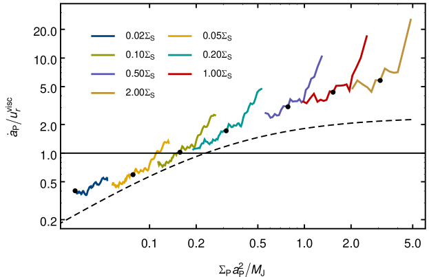
Figure 23: The migration speed, $\dot{a}_{\rm p}$, of a massive Jupiter mass planet through locally isothermal disks with different surface densities. The speed is normalized to the viscous inflow velocity of the disk, $u_{r}^{visc}=3/2\,\nu/r$, where $\nu=\alpha c_{\rm s}H$. Each of the models, as denoted by the different colors has a specific, constant mass accretion rate where the unit surface density, $\Sigma_{\rm S}$, belongs to $\dot{M}=10^{-7}M_{\odot}/$yr. All planets start at unit distance ($r=1$) at the top right end of the individual curves. The black dots refer to the location $r=0.7$ The dashed line refers to the results by 2014ApJ...792L..10D where a globally constant viscosity $\nu$ was used. Figure taken from 2015A&A...574A..52D .

After having looked at the conditions for gap formation we will now analyze the impact on the migration of the planet. For gap opening planets the corotation region will be reduced in mass leading to a lowering of the corotation torques. For larger planet masses the gap widens such that the Lindblad torques will be reduced as well, and the migration rate will be considerably slowed down. Given by the strong lowering in the density (Fig. 22) the perturbations are now nonlinear and the corresponding regime of migration was coined type II migration 1997Icar..126..261W , in order to distinguish it from the previous linear type I regime. The main assumption of type II migration assumes that after having opened an annular gap in the disk, the planet will remain always in the middle of this gap during the migration, i.e. the planet has to move with the same speed as the gap. Because the disk (with its gap) evolves on a viscous timescale it was expected that the planet is coupled entirely to the viscous evolution of the disk 1986ApJ...309..846L and has to move with the same timescale

$$\tau_{\rm mig,II}=\tau_{\rm visc}=\frac{r_{\rm p}^{2}}{\nu}=\frac{r_{\rm p}^{2}}{\alpha c_{\rm s}H}=\frac{1}{\alpha h^{2}\Omega_{\rm p}}\,.$$ (103)

In this type II migration regime the rate is independent of the planet mass, and depends only on disk and stellar parameter. This can only be valid if the disk mass, $m_{\rm d}\approx\pi\Sigma_{0}r_{\rm p}^{2}$, is larger than the planet mass $m_{\rm p}$. Otherwise the planetary inertia will require a reduction factor such that $\tau_{\rm mig,II}=m_{\rm d}/m_{\rm p}\tau_{\rm visc}$ 1999MNRAS.307...79I ; 1995MNRAS.277..758S . Numerical simulations of a migrating Jupiter type planet over long timescales found a good overall qualitative agreement with these expectations 2000MNRAS.318...18N .

Recently however, the assumption (103) has been brought into question and it has been argued that the migration of gap-opening planets is not locked to the viscous evolution of the disk 2014ApJ...792L..10D . By performing sequences of numerical simulations of massive planets in the disk it was found that the migration rate is not given by eq. (103) but can be faster as well as slower than this rate, a feature that was noted already earlier 2007ApJ...663.1325E . The reason for this behaviour lies in the fact that a gap does not separate the inner and outer disk completely as is typically assumed. During the migration of the planet, mass is transferred from one side of the planet to the other side across the planetary orbit and hence the gap will always be dynamically recreated. If the planet migrates faster than the viscous speed then mass is transferred from the inside to the outside and the other way around for migration speeds that are slower than the viscous speed. More recently, models of migrating planets in accreting disks have been constructed 2015A&A...574A..52D and very similar results have been found. As shown in Fig. 23 the typical migration rate of a massive planet can be faster or slower as the viscous rate. From a physical perspective this result was expected because the planet can only be moved through the disk by torques acting on it, such that the actual migration speed is always given by eq. (88).

The total torque acting on a migrating planet can be written as the product of a stationary torque and a dynamical correction factor 2015A&A...574A..52D . The first contribution, the stationary torque $\Gamma_{\rm still}=f_{\rm still}\Gamma_{0}$, refers to the situation of a planet that does not move through the disk but remains at its actual distance from the planet. Here, $\Gamma_{0}$ is the normalization from above, see eq. (94), and $f_{\rm still}$ is a correction factor that depends for a given disk parameter (viscosity, thickness) on the mass of the planet. For smaller mass planets that can be treated in the linear regime, $f_{\rm still}$ is a constant, given for example by eq. (92). However, larger planets clear out a gap such that $f_{\rm still}$ becomes lower 1997Icar..126..261W . Simulations of embedded planets in accreting disks with non-zero $\dot{M}$ have been performed that first keep the planet fixed on its orbit in order to calculate $f_{\rm still}$ 2015A&A...574A..52D . Then the planets were released and the subsequent evolution followed. Interestingly, for locally isothermal disks it was found that the normalized torque $\Gamma/\Gamma_{0}$ was constant during each migration process, which implies that one can write, $\Gamma=f_{\rm mig}\,f_{\rm still}\,\Gamma_{0}$, with a constant $f_{\rm mig}$. This means that the factor $f_{\rm mig}$ does not depend on the local disk mass but only on the planet mass and disk viscosity 2015A&A...574A..52D . It is typically smaller than one, only for rapid type III migration it is larger.

6.4 Other regimes of migration

Having studied the standard form of migration of planets in viscous, laminar disks we will now briefly describe other forms of planet migration that consider more aspects of disk physics that have hitherto been neglected. In addition to the mentioned type I and II migration regimes there exists a regime dominated by rapid, or runaway migration 2003ApJ...588..494M , for which subsequently the new term type III migration 2004pfte.confE...2A ; 2004AGUFM.P32A..06W has been established. Because accretion disks are driven by internal turbulence either hydrodynamically or via a combination with magnetic fields, the gas motion is not laminar but rather shows random fluctuations. The interaction of these variable flow field with embedded planets leads to an additional type of migration, sometimes termed stochastic migration. Finally, in more massive disks the effects of disk self-gravity cannot be neglected anymore and will influence the density structure and subsequently the planet migration process.

Type III migration

In contrast to most of the previous calculations (with the exception of the type II discussion) now the torque acting on a moving planet is considered. Let us focus on a planet undergoing inward radial migration on a circular orbit. Material located in the vicinity of the separatrix, between inner disk material that is on circulating streamlines and material on librating horseshoe orbits, will undergo a single U-turn upon a close encounter with the planet and will cross the entire horseshoe region. In doing so, it will directly move from the inner to the outer disk and not be trapped in the horseshoe region. This transfer of disk material from one side of the planet to the other implies an exchange of angular momentum with the planet. The inner material that crosses horseshoe gains angular momentum that the planet has to loose. The exerted torque can be written as 2012ARA&A..50..211K

$$\Gamma_{\rm flow}=2\pi\,\Sigma_{\rm s}\,\dot{r}_{\rm p}\Omega_{\rm p}r_{\rm p}^{3}x_{\rm s}\,,$$ (104)

where $x_{\rm s}$ is the width of the horseshoe region and $\Sigma_{\rm s}$ the surface density at the inner separatrix. This ”flow-through corotation torque” depends on the migration speed, $\dot{r}_{\rm p}$, of the planet, and there is a positive feedback between the migration rate and the torque, i.e. the torque increases with the migration speed. Hence, in principle this can lead to a runaway migration 2003ApJ...588..494M ; 2004ASPC..324...39A . More detailed analysis 2003ApJ...588..494M shows that the efficiency of the migration will depend on the mass contained within the horseshoe region. This is because the planet has to carry this material with it upon migrating inward which acts as additional inertia that will tend to counteract the runaway process. On the other if the horseshoe is too empty, i.e. the planet too massive, there will be too little material left over ($\Sigma_{\rm s}$ too small) to drive fast migration. The results show that the highest efficiency requires a partially emptied horseshoe region, where the difference between the mass that would be contained in the horseshoe region if the disk was unperturbed by the planet and the mass that is actually contained in this region (sometimes called coorbital mass-deficit, $\delta m$) equals the planet mass. For the MMSN the most promising planet mass for type III migration lies in the Saturn mass range beyond a distance of about 10 AU. An increase in disk mass will enhance the runaway migration such that disks that are prone to type III migration are always close to being at the limit of gravitational instability 2003ApJ...588..494M . Due to the symmetry implied by eq. (104) the direction of type III migration can be directed inward or outward, depending on the initial perturbation to the planet’s motion. This feature has been demonstrated explicitly by numerical simulations 2008MNRAS.387.1063P ; 2008MNRAS.386..179P , where is was also shown that even massive planets of a few Jupiter masses can enter the rapid type III migration regime. The fast migration terminates when the planet moves into disk conditions that do no longer favor type III migration, i.e. the coorbital mass deficit, $\delta m$, no longer matches approximately the planet mass. During type III migration not only the planet itself has to be moved very fast through the disk but all of the material that resides bound to the planet within its Hill sphere. For massive planets this material is stored in a circumplanetary disk orbiting the planet and hence the details of type III efficiency will depend on the total mass within this disk 2008MNRAS.387.1063P ; 2008MNRAS.386..179P . Type III migration may have played an important role during the early evolution of the Solar System, as a potential driving mechanism for motions of Saturn and Jupiter with the Grand Tack scenario 2011Natur.475..206W . The fact that type III migration is more efficient for massive disks takes us directly to a discussion of migration in disks where self-gravity can play a role.

Migration in disks with self-gravity

In situations where the total mass of the disk, $m_{\rm disk}$, is no longer negligible with respect to the star, $M_{*}$, it is not anymore sufficient to consider only the gravitational potential of the star but one has to add a contribution from the disk, i.e. consider an additional term from the disk’s self-gravity $\Psi=\Psi_{*}+\Psi_{\rm d}$, where the latter is given by an integral over the whole disk (53). This change in the potential leads to a (slightly) different angular velocity of the disk that is now no longer Keplerian. In turn this leads to a radial shift in the location of the Lindblad resonances between the Fourier components of the planet and the disk material, see eq. (91). As the torques on an embedded planet can be calculated in linear theory by summing over different resonances one may expect a change in the migration rate for embedded planets 2005A&A...433L..37P ; 2008ApJ...678..483B . Typical planet migration simulations with a ’life planet’ that is allowed to move freely according to the gravitational forces of the disk assume that only the planet feels the disk’s gravity but not the disk itself, i.e. neglect the disk’s self-gravity. As pointed out 2008ApJ...678..483B , this is obviously an inconsistent situation, because planet and disk move in different gravitational fields. Through direct 2D-hydrodynamical simulations that include the disk’s self-gravity they showed that for a disk only 3 times the MMSN this inconsistency may lead to a difference in the torque and hence migration rate by a factor of 2. They point out that a self-consistent simulation can be constructed easily by omitting the axisymmetric contribution of the density in calculating the force on the planet. By including the effects of disk self-gravity in the linear calculations it was found that for disks a few times the MMSN the change in the torque is only about 10% of that in a non-self-gravitating disk 2005A&A...433L..37P ; 2008ApJ...678..483B . This difference can be accounted for by the radial shift in the Lindblad resonances, leading to a migration rate is slightly enhanced over the standard value.

In the past years hydrodynamical simulations following the evolution of massive planets embedded in more massive disks have been presented in 2D 2011MNRAS.416.1971B and 3D 2011ApJ...737L..42M . These simulations assume that a planet might have formed by gravitational instability at larger distances in the disk and then migrated to its present location. In the simulations presented in 2011MNRAS.416.1971B the disk setup is chosen such that they are marginally stable, i.e. have a Toomre number of about $Q\sim 2$ in the main part. Under these conditions the disk does not fragment into individual blobs but generates stochastic spiral disturbances that can produce an effective viscosity and a heating of the disk. This heat is assumed to be radiated away from the disk surfaces, a process modeled by a radially varying cooling function, where the cooling time is given by $\tau_{\rm cool}=\beta\Omega^{-1}$, so called $\beta$-cooling, see eq. (74). Hence, a statistically stationary disk setup can be produced where the effective viscosity, as generated by the gravo-turbulent fluctuations of the disk, is given by

$$\alpha_{\rm sg}=\frac{4}{9}\,\frac{1}{\gamma(\gamma-1)\beta}\,.$$ (105)

This relation can quite generally be derived 2001ApJ...553..174G just by assuming that the turbulent heat generated acts like a viscous dissipation $\propto\Sigma\nu(d\Omega/dr)^{2}$ which is balanced by the local cooling $de_{\rm th}/dt\propto e_{\rm th}/\tau_{\rm cool}$, with the thermal energy density $e_{\rm th}$, see section 5.3. And this is independent of the source of the turbulence. For a value of $\beta=20$ 2011MNRAS.416.1971B found in their simulations an $\alpha_{\rm sg}\approx(2-3)\cdot 10^{-2}$ in agreement with the expectation (105). Then massive planets are embedded in these disks at large distances (about 100 AU) and their subsequent evolution is followed through 2D hydrodynamical calculations. The simulation show that the planets experience a very rapid inward migration. For example, a Jupiter mass planet embedded into a disk with aspect ratio $h=0.1$ ($\beta=20$) migrated within less than $10^{4}$ yrs from 100 AU all the way to only $20$AU. This fast migration is somewhat reminiscent to the type III migration that was discussed earlier. However, the planets do not open up a clear gap such that the coorbital mass deficit equals the planet mass, because the gap opening times are longer than the migration timescale. Hence, the migration is basically of type I with stochastic episodes superimposed, that allow even for brief phases of outward migration. These results have been supported by full 3D simulations of migrating Jupiter type planets 2011ApJ...737L..42M where a Jupiter planet embedded at 25AU into a $0.14M_{\odot}$ disk plunges in only $10^{3}$ yrs to 6AU. These short migration timescales of clumps formed in more massive disks represent a serious challenge to planet formation via gravitational instability scenario 2012ApJ...746..110Z , as shown in the previous section.

Stochastic migration

As pointed out already just above, planets embedded in a disk that exhibits turbulent fluctuations will display not a monotonous smooth migration but will experience stochastic fluctuations in their actual migration rate. To study this process under realistic conditions, numerical simulations of turbulent disks with embedded planets have been performed using full magneto-hydrodynamical (MHD) computations in 3D. Magnetized disks are susceptible to the magneto-rotational instability (MRI) which is believed to be responsible for responsible for driving accretion at least in sufficiently ionized disks 1991ApJ...376..214B ; 1991ApJ...376..223H . Several direct simulations of planets embedded in turbulent discs have been performed for the case of MRI unstable discs 2004MNRAS.350..849N ; 2005A&A...443.1067N ; 2011ApJ...736...85U . In MHD simulations with embedded low mass planets (up to 30 $M_{\rm Earth}$) is was found that the planets experience a random walk process where on average the migration resembles standard type I inward migration, however, with possible long term ($\sim$ 100 orbits) phases of outward migration 2004MNRAS.350..849N . The fluctuation can also lead to a non-zero eccentricity of the embedded planets of the order of a few percent 2005A&A...443.1067N . For a Jupiter mass planet it has been found that the gap is somewhat wider than in the corresponding laminar case using the same effective $\alpha$-value for the disk 2011ApJ...736...85U ; 2012ARA&A..50..211K . Here, the (relative) turbulent fluctuations become weaker and the migration resembles that of standard laminar disks. For intermediate planet masses, phases of sustained outward migration have been reported 2011ApJ...736...85U . In simulations with very low planet masses (a few $M_{\rm Earth}$) is was found 2011A&A...533A..84B that the structure of the (averaged) flow in the corotation region in full MHD simulations is comparable to the laminar results, indicated the presence of corotation torques also in turbulent magnetic disks. To circumvent the expensive full 3D magnetohydrodynamical simulations, approximate treatments have been developed where the random features of the MHD turbulence is modeled by stochastic forces that can be added in standard hydrodynamical simulations 2004ApJ...608..489L ; 2010ApJ...709..759B . We will no go into more details at this point but rather refer to other review articles 2012ARA&A..50..211K ; 2014prpl.conf..667B .

6.5 Eccentricity and inclination

In addition to a change in the distance from the central star, embedded planets will suffer a change in the other orbital elements as well. Most important here are the eccentricity and inclination evolution. The circular and coplanar orbits in the Solar System were taken already early on, for example by Kant and Laplace 1755anth.book.....K ; 1776Laplace , as evidence that the planets form in a flat disk-like configuration. The growing sample of extrasolar planets with their huge variety in orbital elements has shown that a large fraction of planets display significant orbital eccentricity and some systems show a large tilt with respect to the stellar rotation axis, that is expected to be aligned approximately with the rotation axis of the protoplanetary nebula. The question arises whether these orbital characteristics of the extrasolar planets can be a result of disk-planet interaction or have another dynamical origin.

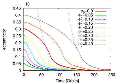
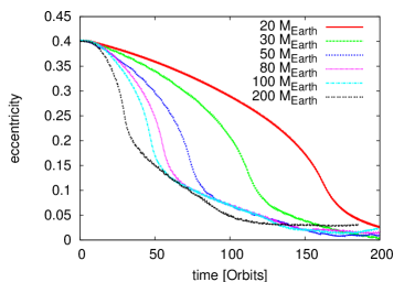
Figure 24: The change in eccentricity of an embedded planet due to planet-disk interaction. The disk models have been calculated using full 3D radiation hydrodynamical simulations. Left panel The change in eccentricity of a $m_{\rm p}=20M_{\rm Earth}$ planet for various initial eccentricities. The planet mass is switched on gradually during the first 10 orbits (vertical dotted line). The dashed lines indicate exponential decay laws. Right panel The change in eccentricity of planets with different masses all starting from the same initial eccentricity, $e_{0}=0.4$. Figure taken from 2010A&A...523A..30B .

Eccentricity

In calculating the change of the eccentricity of the planet, we have to start from the angular momentum and energy of a planet orbiting the star. These are given by

$$J_{\rm p}=m_{\rm p}\,\sqrt{GM_{*}a}\,\sqrt{1-e^{2}}\quad\text{and}\quad E_{\rm p}\,=\,-\,\frac{1}{2}\,\frac{GM_{*}m_{\rm p}}{a}$$ (106)

where we dropped the subscript and wrote for simplicity just $a$ and $e$ for the planetary semi-major axis and eccentricity, respectively. Classical mechanics tells us that the angular momentum is changed by the torque and the energy by the power acting on the planet by the disk. These are given by

$$\Gamma_{\rm disk}=-\int_{\rm disk}\Sigma\,\left.(\vec{r}_{\rm p}\times\vec{F})\,\right|_{z}\,df\quad\text{and}\quad P_{\rm disk}\,=\,\int_{\rm disk}\,\Sigma\,\dot{\vec{r}}_{\rm p}\cdot\vec{F}\,df\,,$$ (107)

where $\Gamma_{\rm disk}$ was defined already before in eq. (86). The changes in $E_{\rm p}$ and $J_{\rm p}$ are now given as

$$\frac{\dot{J}_{\rm p}}{J_{\rm p}}=\,\,\frac{1}{2}\frac{\dot{a}}{a}-\frac{e^{2}}{1-e^{2}}\frac{\dot{e}}{e}\ =\frac{\Gamma_{\rm disk}}{J_{\rm p}}$$ (108)

and

$$\frac{\dot{E}_{\rm p}}{E_{\rm p}}=\,\,-\frac{\dot{a}}{a}\ =\frac{P_{\rm disk}}{E_{\rm p}}\,.$$ (109)

Having calculated $\Gamma_{\rm disk}$ and $P_{\rm disk}$ from the simulations, one can directly evaluate the changes in the orbital elements of $a$ and $e$. Obviously, the change in the semi-major axis is given solely by $P_{\rm disk}$ and not by the torque as assumed above in eq. (88). The reason for this apparent discrepancy lies in the fact that we assumed circular orbits in the discussion in section 6.1. Setting $e=0$ we find from eqs. (108) and (109) that $P_{\rm disk}=\Omega_{\rm K}\,\Gamma_{\rm disk}$ such that for circular orbits one can use indeed the torque to estimate the migration rate.

For low mass planets that do not open a significant gap within the disk, linear perturbation theory can be applied to analyze the eccentricity evolution. In contrast to the circular case an eccentric planet generates additional resonances in the disk 1980ApJ...241..425G . Similar to a planet on a circular orbit, Lindblad resonances occur at disk locations where the perturbation frequency experienced by a fluid element equals the local epicyclic frequency, and corotation resonances occur wherever the pattern speed equals the local angular velocity of the disk. External Lindblad resonances act to increase $e$, while corotation and co-orbital Lindblad resonances act to damp it 2003ApJ...585.1024G . The outcome depends on the relative contribution of damping and exciting contributions and, similar to the migration, and the net result is the (small) difference of larger individual contributions. Linear analyses shows that (for not too high initial values) the eccentricity is damped exponentially on a timescale much shorter than the migration timescale, where typically

$$\tau_{\rm ecc}\sim\left(\frac{H}{r}\right)^{2}\,\tau_{\rm mig}\,.$$ (110)

Equation (110) applies for initial eccentricities smaller than the relative scale height, $e\lesssim H/r$ 2004ApJ...602..388T . This rapid decline in $e$ is caused primarily by the damping action of the corotation resonances. For larger initial eccentricities with $e\gtrsim H/r$ the increased speed of the planet with respect to the disk material makes the interaction nonlinear and the damping rate changes to 2000MNRAS.315..823P

$$\frac{de_{\rm p}}{dt}\propto-\,e_{\rm p}^{-2}\,.$$ (111)

These results on the evolution of $e_{\rm p}$ (here we added the subscript ’p’ for clarity), including the turnover from the exponential to the quadratic damping in eq. (111), have been confirmed through full non-linear multi-dimensional hydrodynamical simulations of embedded low-mass planets up to 30$M_{\rm Earth}$ in 2D disks 2007A&A...473..329C and up to 200 $M_{\rm Earth}$ in 3D radiative disks 2010A&A...523A..30B . In Fig. 24 we display the time evolution of the planetary eccentricity with time for different initial eccentricities (left panel) and different planet masses (right panel). From the time evolution it is clear that decay rate is indeed different for large and small $e_{\rm p}$, it changes from that of eq. (111) to the exponential rate at the turnover eccentricity of $e_{\rm p}\approx 0.1$ which is equivalent to is $e_{\rm p}\approx 2H/r$. The same behaviour was found in the 2D simulations as well 2007A&A...473..329C . The right panel of Fig. 24 shows that the damping rate increases with increasing mass of the planet, at least for large initial $e_{\rm p}$. This behaviour is in conflict with theoretical expectations based on linear theory that there should be a regime where eccentricity excitation due to planet disk interaction is possible 2003ApJ...585.1024G . The authors argue that the damping effect of the corotation region diminishes when the planet becomes massive enough to open a gap. Hence, they expect a possible eccentricity excitation for planet masses around Saturn or Jupiter. However, the results displayed in Fig. 24 from 2010A&A...523A..30B and more recent 3D simulations 2013MNRAS.428.3072D indicate otherwise. Only for very large planets with masses beyond 10 $M_{\rm Jup}$ planet disk interactions will lead to a significant rise in the $e_{\rm p}$ 2001A&A...366..263P ; 2006ApJ...652.1698D . This increase in the planet’s eccentricity is caused in that case by the back-reaction of an eccentric disk on the embedded planet where the disk’s eccentricity has been generated by the presence of the planet 2006A&A...447..369K . However, very recent simulations have hinted at possible eccentricity growth for massive planets in disks with low viscosity and small pressure 2015ApJ...812...94D , demonstrating that more studies are required to settle this issue. Nevertheless, the numerical results indicate that the observed high eccentricities in the extrasolar planets cannot in general be the outcome of planet-disk interaction but are rather a result of multi-body gravitational interactions.

Inclination

Similar to the eccentricity changes, the disk’s impact on the inclination has been studied through linear analyses 2004ApJ...602..388T which indicate that for low inclinations with $i_{\rm p}\lesssim H/r$ the inclination is exponentially damped, i.e. $di_{\rm p}/dt\propto-i_{\rm p}$. The decay occurs again on a timescale that is of the same order as the eccentricity damping time, i.e. by a factor $(H/r)^{2}$ shorter than the migration timescale. The exponential decay for the inclination has been supported in 3D hydrodynamical simulations of planets embedded in isothermal disks 2007A&A...473..329C . For larger inclinations $i_{\rm p}\gtrsim H/r$, these researchers find inclination damping on a longer timescale with a behavior $di_{\rm p}/dt\propto\,-\,i_{\rm p}^{-2}$ which is identical to the scaling obtained for eccentricity damping when $e_{\rm p}$ is large. This has been verified in full 3D radiative simulations 2011A&A...530A..41B . The different damping rate for larger inclinations is caused by the fact that for inclined orbits with $i_{\rm p}\gtrsim H/r$ the planets leave the disk region vertically twice for each orbit. The damping action of the disk is massively reduced and can only operate during the short time intervals while the planet is crossing the disk. This process can then be treated by a dynamical friction approach 2012MNRAS.422.3611R . Additionally, it has been shown that the inclination is damped by disk-planet interaction for all planet masses up to about $1M_{\rm Jup}$ 2011A&A...530A..41B ; 2009ApJ...705.1575M . In recent 3D simulations of planet-disk interaction for massive, inclined planets it has been shown that the inclination seems typically damped, however with a damping timescale that increases for larger initial inclinations 2012MNRAS.422.3611R ; 2013MNRAS.431.1320X ; 2013A&A...555A.124B .

In summary, due to the much shorter timescales of eccentricity and inclination damping in contrast to the migration time, it is to be expected that for isolated planets embedded in disks these quantities should be very small, at least in laminar disks; i.e., even if planets formed in disks with non-zero $e_{\rm p}$ and $i_{\rm p}$, they would be driven rapidly to a state with $e_{\rm p}=0$ and $i_{\rm p}=0$.

Growing planets that are still embedded in the disk experience gravitational forces due to the interaction with the disk that change the orbital parameter of the planet. Most important is the radial migration of the planet as this implies that the locations where planets are observed today do not necessarily coincide with their formation locations. Initial results (for isothermal disks) indicated very rapid inward migration such that too many planets would have been lost into the star. Recent results have shown that migration can in fact be directed inward or outward, depending on the physical parameters of the disk. On the other hand, eccentricity and inclination are typically damped on much shorter timescales. Hence, the large eccentricities and inclinations of the observed exoplanets are most likely not caused by planet-disk interaction but have their origin in multi-body dynamical interactions.

7 Multi-body systems

So far we have studied the growth and evolution of single planets in the disk. However, the observations indicate that planets tend to be found in systems with several objects rather than being lonesome travelers. In fact, through the Kepler space-mission hundreds of transiting multi-planet systems were discovered 2014ApJS..210...19B . Out of the 1200 planetary systems observed by now (mid 2015), about 500 are multiple planet systems (source: exoplanet.eu). The occurrence and architecture of planetary systems has nicely been reviewed in 2015ARA&A..53..409W .

The presence of additional objects in the system induces gravitational disturbances that can modify the evolution of the individual planets as well the overall evolution of the whole system. This can lead to planets with extreme orbital elements such as high eccentricity or inclination and to the formation of resonant planetary systems. Furthermore, planets are found in binary star systems where their formation pathway is made more challenging through the additional strong gravitational disturbance by the companion star.

In this part we will discuss the dynamics of multi-planet systems, with some focus on the formation of resonant, or near resonant systems, as well as planets in binary star systems.

7.1 Resonances

When talking about resonances, in the context of these lecture notes we will restrict ourselves to mean motion resonances (MMRs) which are defined by an integer ratio of the mean orbital motions of two planets,

$$n_{1}/n_{2}=p/q\quad\quad\mbox{with}\quad\quad q,p\in\mathbb{N}_{>0}\,,$$ (112)

where $n_{i}$ denotes the mean orbital velocity of the $i$-th planet. We will denote the inner planet by $i=1$ and the outer one by $i=2$, hence $p>q$. The order $m$ of the resonance is given by

$$p=q+m\,.$$ (113)

Among the 8 planets in the Solar System there is no MMR. Taking into account the dwarf planets, one finds that Neptune and Pluto are in fact engaged in a 3:2 MMR, where the orbital period of Neptune is 165 yrs and that of Pluto 248 yrs, and their semi-major axes are 29.7 AU and 35.5 AU, respectively. This means that for 3 orbits of Neptune, Pluto performs exactly 2 orbits around the Sun. The high eccentricity of Pluto’s orbit ($e_{\rm P}=0.25$) implies that Pluto’s perihelion lies inside the orbit of Neptune such that the two orbits are actually crossing each other. In general, planetary orbits are only stable if the two planets never approach each other to a distance closer than their mutual Hill radius. For crossing orbits, this condition can only be satisfied if the orbits are resonant. Hence, Pluto’s orbit is protected from being unstable by the special 3:2 resonance that avoids close encounters and maximizes Pluto’s separation from Neptune. For the Pluto-Neptune system additional stabilization arises from the fact that their orbits are mutually inclined by about 17^∘. The fact that the orbit of Pluto is shared by many other plutinos has led eventually to the degradation of Pluto from full planet to dwarf planet status, as decided by the International Astronomical Union in 2006. Similarly, in an exoplanetary system resonances are a way to protect the system from dynamical instability.

To specify a particular resonant configuration of a system, it is useful to define the resonant angles $\Phi_{k}$ by

$$\Phi_{k}=p\lambda_{2}-q\lambda_{1}-p\varpi_{1}+q\varpi_{2}-k(\varpi_{2}-\varpi_{1})\,,$$ (114)

with $p>q$. In eq. (114) the $\lambda_{i}$ denote the mean longitudes and $\varpi_{i}$ the longitudes of periapse of two planets. The integers $k$ satisfy $q\leq k\leq p$ and can take $p-q+1$ possible values. Of the $p-q+1$ resonant angles, at most two are linearly independent, and a resonance condition is given if at least one angle will librate, i.e. its values do not extend over the whole range of 360 degrees but is limited to a smaller range. Let us take as an example a system with a 2:1 resonance. Here, $p=2$ and $q=1$, such that we have

$$\Phi_{1}=2\lambda_{2}-\lambda_{1}-\varpi_{1},\quad\Phi_{2}=2\lambda_{2}-\lambda_{1}-\varpi_{2}\quad\quad(\Delta\varpi=\Phi_{2}-\Phi_{1})\,,$$ (115)

where we defined as an additional variable the difference $\Delta\varpi$ (sometimes also $\Phi_{1}-\Phi_{2}$) between the longitudes of periapse which is often used to replace one of the resonant angles $\Phi_{1}$ or $\Phi_{2}$. The resonant angles $\Phi_{k}$ follow from an expansion of the perturbation potential between the two planets that would move otherwise on unperturbed Kepler-orbits. Upon expanding the perturbation in a Fourier-series, the resonant angles are the stationary phases in the expansion. If an angle $\Phi_{k}$ is in libration (i.e. covers a range smaller than $[0,2\pi]$), then the system is said to be in a MMR. For more detailed information of resonances see the excellent book of Solar System Dynamics by Murray & Dermott 1999ssd..book.....M . For a 2:1 resonance, if both angles $\Phi_{k}$ librate (i.e. $\Delta\varpi$ as well), then the system is said to be in a state of apsidal corotation resonance (ACR), where the two lines of periapse rotate with the same speed (on average) 2003ApJ...593.1124B . For Keplerian orbits the resonant condition (112) for two planets implies a ratio of their semimajor axes of $a_{2}/a_{1}=(n_{1}/n_{2})^{2/3}$, which follow from Kepler’s third law.

One of the most famous examples of a planetary system in a first order 2:1 resonant configuration is GJ 876. The initial discovery 2001ApJ...556..296M noted two massive planets (GJ 876 b and c) with minimum masses of $0.56$ and $1.89M_{\rm Jup}$ that orbit a M-type star of only 0.3 $M_{\odot}$. These two planets have periods of 30 and 60 days and their orbits are fully aligned, i.e. $\Delta\varpi$ is in libration with $\Delta\varpi_{\rm max}\approx 30^{\circ}$ 2001ApJ...556..296M , hence GJ 876 is in an ACR state. Another example is the system HD 128311 where two massive planets are again in a 2:1 resonance but here only one resonant angle is librating, while the second one is circulating, hence the system is not in an ACR state 2005ApJ...632..638V . A system that is believed to be in a second order 3:1 resonance is HD 60532 where two massive planets orbit an F-type star 2008A&A...491..883D .

Later two additional planets have been discovered in GJ 876, one (d) very close-in on a 2d orbit around the host star, and another fourth Uranus mass planet (e) in a 124 day orbit beyond planets b and c. This places the three outer planets of GJ 876 in a Laplace-type 4:2:1 configuration 2010ApJ...719..890R . This first known resonant chain amongst extrasolar planets bears some similarity to the Laplace resonance of the Galilean satellites Io-Europa-Ganymede orbiting Jupiter but it is dynamically very different as it exhibits a longterm chaotic dynamics 2010ApJ...719..890R ; 2013MNRAS.433..928M . Another famous example of a planetary system that is believed to be in a 3-body Laplace resonance is the directly imaged system HR 8799 where three massive planets are orbiting a young A-star 2014MNRAS.440.3140G . During the last years more resonant chains have been discovered using Kepler-data. In Kepler-60 three planets with masses around $\sim 4$M_⊕ are engaged in a 5:4:3 Laplace MMR 2016MNRAS.455L.104G . The four Neptune mass planets in Kepler-223 have periods in a ratio close to 3:4:6:8 2016Natur.533..509M . This four planet resonant chain has been taken as another clear indication that migration of planets through the disk must have taken place.

Formation of resonant planetary systems

A resonant configuration between two planets is a special dynamical state and it is not very likely that the two planets formed directly in situ at their observed locations, or were captured into such a state. Instead, the formation of resonant planetary systems is a natural outcome of a differential migration process. Here, it is assumed that several planets form in a disk and migrate according to the torques acting on them. Typically, the radial drift speeds are not identical and a differential migration process ensues. In case the inner planet migrates slower than the outer one, the radial distance between the two planets becomes smaller and they approach each other. Whenever the location of a resonance is crossed, i.e. the current orbital periods of the planets have an integer ratio, the mutual interaction becomes stronger due to the periodic perturbations. As a consequence the planets can be trapped in a resonance that is maintained during the subsequent migration process. A typical situation of such a process is shown in Fig. 25, which shows the surface density distribution of a disk with two massive embedded planets, obtained from a numerical model that simulates the formation of the system HD 73526 2007A&A...472..981S . Because the planets are relatively close, they orbit within a joint deep gap where the outer planet feels only the torque by the outer disk (which is negative) and the inner planet feels only the torque of the inner disk (which is positive). Consequently, the two planets approach each other and a convergent migration process sets in, and eventually the planets are captured in a resonance, here 2:1. In the subsequent migration process the planets maintain the resonance and move jointly together towards the central star. The resonant capture is accompanied by an increase in the orbital eccentricities of the planets. The evolution of the semimajor axis and eccentricity for such a resonant capture process is displayed in Fig. 26.

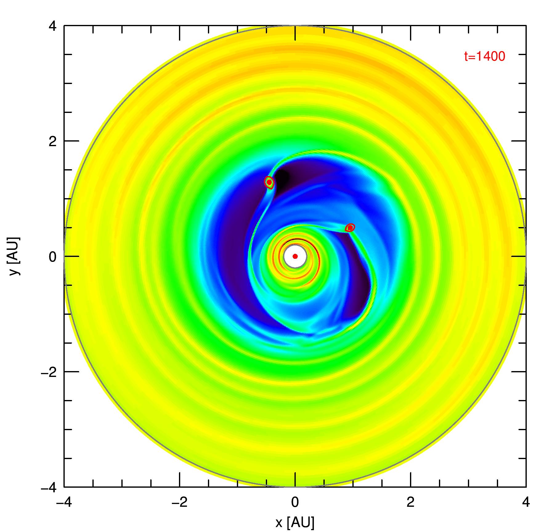
Figure 25: Outcome of a two-dimensional hydrodynamical simulation of two embedded planets in a protoplanetary disk, for parameters of the system HD 73526 where two planets of about 2.5 $M_{\rm Jup}$ each orbit a central star. Shown is the gas surface density where yellow denotes higher density and blue lower values. The central red dot denotes the position of the star while the locations of the planets are given by the two red dots and the red lines indicate their Roche lobes. The scale of the $x,y$ axes is in AU. Shown is the configuration 1400 yrs into the simulations after capture in a 2:1 resonance has occurred, see Fig. 26. After 2007A&A...472..981S

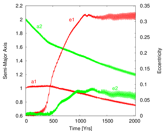
Figure 26: The evolution of the semi-major axes and eccentricities of two embedded planets in a disk (those shown in Fig. 25) for a full hydrodynamical model. The semimajor axis and eccentricity of the inner planet ($a_{1}$ , $e_{1}$) are indicated by the red curves and of the outer planet ($a_{2}$ , $e_{2}$) by the green curves. Starting from their initial positions ($a_{1}=1.0$ and $a_{2}=2.0$ AU) the outer planet migrates inward (driven by the outer disk) and the inner one very slowly outward (due to the inner disk). After about 400 yrs into the simulations they are captured in a 2:1 mean motion resonance and they remain coupled during their inward migration. The eccentricities increase rapidly after resonant capture and settle to equilibrium values for longer times.

The modeling of the resonant capture process is very time consuming because multi-dimensional hydrodynamic simulations have to be performed, and a full evolution takes typically several weeks to run due to the long evolutionary times to be simulated. Hence, a simple model for this type of process, using only 3-body simulations consisting of one star and two planets has been suggested where the action of the disk is taken care of by adding additional damping forces using a parameterization of the migration and eccentricity damping. This type of a modeling takes only a few minutes. Specifically, the following prescription for the time evolution of the semi-major axis, $a$, and eccentricity, $e$, of embedded planets has been used in simulations performed to explain the observed state of GJ 876 2002ApJ...567..596L

$$\frac{\dot{a}}{a}=\frac{1}{\tau_{\rm a}},\quad\frac{\dot{e}}{e}=\frac{1}{\tau_{\rm e}}\equiv K\,\frac{\dot{a}}{a}\,.$$ (116)

Here $\tau_{\rm a}$ and $\tau_{\rm e}$ denote the damping time scales for the semi-major axis and eccentricity of the planets, respectively, and $K$ is a constant that describes the ratio between these two. This prescription for $\dot{a}$ and $\dot{e}$ can be used in principle for both planets because they are both in contact with the disk, but often it is applied only to the outer one assuming that the inner disk has been accreted already onto the star. The parameter $K$ specifies the ratio of migration and eccentricity damping. In a study to model GJ 876 Lee & Peale 2002ApJ...567..596L have applied exactly this model (damping of the outer planet only) and showed that a configuration similar to the observed one can be obtained by choosing a value $K=100$ for the eccentricity damping. Smaller values for $K$ typically result in too small damping and instability of the system. In follow-up studies, using full hydrodynamic simulations it was found that the disk damping for these systems with massive planets will produce values of $K\sim 10$ only 2004A&A...414..735K . Later it was shown that by taking the inner disk into account, as displayed in Fig. 25, it is possible to obtain full hydrodynamic results in agreement with the observed state of GJ 876 2008A&A...483..325C . The system ends up in apsidal corotation, with correct eccentricities.

This type of differential migration process is a very natural outcome of the dynamical evolution of planets embedded in protoplanetary disks, and very many resonant configurations should be expected, the only question remaining, in which resonance are the planets captured. To become captured in a resonance the migration has to be sufficiently slow such that the excitation mechanism can operate long enough for them to be captured. If the migration is too fast, the planets cross the resonance and the system becomes more unstable. In addition the interaction between the two planets has to be strong enough for capture. As a consequence, massive planets in the Jupiter mass range and larger are typically captured into a 3:1 or 2:1 resonance 2004A&A...414..735K . In fact observationally there is indeed a clustering of massive planets within the 2:1 resonance 2015ARA&A..53..409W . On the other hand, for smaller mass planets, where the outer planet has up to a Saturn mass are typically captured into a 3:2 resonance 2008A&A...482..333P .

Figure 27: Histogram of the number of two adjacent planets with a given period ratio for multi-planet system. The overall distribution is smooth but enhancements are visible near the 3:2, 2:1 and 3:1 resonances. After 2015ARA&A..53..409W

Given that embedded planets have to migrate through the disk due to the disk torques and given that resonant capture is a very probable outcome during the evolution, then the small number of extrasolar planet pairs actually being in resonance is quite surprising. Indeed, the observed distribution of period ratios between two adjacent extrasolar planets is relatively smooth and does show only a mild enhancement of planet pairs near the mostly expected 3:2 and 2:1 resonances. Considering the turbulent nature of the protoplanetary disk the migration process is not smooth anymore but has a random component due to the gravitational disturbances of individual turbulent eddies. Through a large set of $N$-body simulations taking disk turbulence into account it was shown that the overall distribution of the period ratios (see Fig. 27 for the observational data) seems to be in rough agreement with standard migration including stochastic forces 2012MNRAS.427L..21R . This is in agreement with results showing that stochastic perturbations can break the resonances between two planets 2008ApJ...683.1117A . This breaking of resonances allows for the possibility of bringing two planets very close together and producing systems of closely spaced low-mass planets. For the system Kepler-36 it was shown that this mechanism may be responsible to explain the unusually close configuration near the high degree first order 7:6 mean motion resonance 2013MNRAS.434.3018P .

Another feature apparent in Fig. 27 is the fact that the over abundances of period ratios near the 2:1 and 3:2 resonances do not occur at exact resonance position but lie just outside of it, a fact noticed earlier 2013AJ....145....1B . It has been argued that this small shift of period ratios just outside of the nominal values may be the result of resonant repulsion or dissipative divergence in the presence of tidal dissipation within the inner planet 2012ApJ...756L..11L ; 2013AJ....145....1B . Recently, it has been argued however, that tides alone cannot be held responsible for this enhancement near the 2:1 resonance, because this would imply too large initial eccentricities 2015MNRAS.453.4089S . Another recent suggestion is the interaction of the planets with the remaining planetesimal disk. Here, it has been found that for the case of a sufficiently massive planetesimal disk the resonances can be disrupted and planet system remains just outside of the nominal values during the subsequent evolution 2015ApJ...803...33C .

7.2 Dynamics

Already after the first detections of extrasolar planets it was noted that they display a large variation of orbital eccentricities similar to spectroscopic binaries 2007ARA&A..45..397U . Both $e$-distributions cover the whole range from $0\leq e\leq 1$ and have high mean values (with $e\sim 0.3$) in obvious contrast to the Solar System where the majority of the bigger planets (despite Mercury and Mars) have a rather small eccentricity. For the overall $e$-distribution the following form has been suggested 2008ApJ...685..553S

$$\frac{dN}{de}\propto\left(\frac{1}{(1+e)^{b}}-\frac{e}{2^{b}}\right)\,,$$ (117)

where $dN$ is the number of planets in an eccentricity interval $[e,e+de]$. According to 2008ApJ...685..553S $b=4$ gives a good match to the observed distribution which gives a smooth distribution which peaks at $e=0$. There is a tendency for lower mass planets to have a lower eccentricity, in particular for $m_{\rm p}<50M_{\rm Earth}$ the maximum eccentricity is around $e\approx 0.4$ while larger mass planets reach over $e>0.9$. This finding is in agreement with the fact that lower mass planets are preferentially found in multi-planet systems that have on average lower eccentricities. For an overview of the observational properties and more references see 2015ARA&A..53..409W .

In the previous section 6 we showed that planet-disk interaction will typically lead to eccentricity and inclination damping on a timescale shorter than the migration time. Consequently, planet-disk interaction cannot be responsible for the observed eccentricity distribution and two other processes (planet-planet scattering or the Kozai-mechanism) have been suggested that both require additional objects. In the first scenario several planets have formed in the disk and undergo initially a convergent migration process which leads to a compact configuration either in resonance or close to it. Upon disk dissipation its stabilizing effect disappears and the planetary system my become dynamically unstable. This will increase the eccentricity and inclination of the objects leading eventually to a scattering processes 2003Icar..163..290A . Some bodies will be scattered towards the star and some outwards, or be thrown out altogether. As shown by several simulations using many realizations of such models, these type of planet-planet scattering processes can lead to eccentricity distributions very similar to the one observed for the ensemble of extrasolar planets 2008ApJ...686..621F ; 2008ApJ...686..603J .

Figure 28: The geometry of a hierarchical 3-body system susceptible to the Kozai-mechanism. A binary system with masses $m_{0}$ and $m_{1}$ is orbited by a third object $m_{2}$ that is on an inclined orbit. The inclination of the two orbital planes is initially $I_{0}$. Please note that the distance (semimajor axis) of the third object ($m_{2}$) is much larger than that of the secondary object ($m_{1}$) so the real orbits do not intersect.

The Kozai mechanism

In the past 20 years or so a dynamical process operating in a hierarchical 3-body system has gained much of attention to explain certain properties of extrasolar planetary systems. The mechanism was originally proposed to explain the dynamics of main-belt asteroids due to the perturbations of Jupiter by Y. Kozai 1962AJ.....67..591K . The geometry of a hierarchical system is sketched in Fig. 28. A central 2-body system with masses $m_{0}$ and $m_{1}$ is orbited by a third object ($m_{2}$) at a larger distance, $r_{2}>r_{1}$. The two orbital planes are inclined by a certain angle $I$ with each other. Such a configuration describes for example the asteroid case in the Solar System, where: $m_{0}$ = Sun, $m_{1}$ = asteroid and $m_{2}$ = Jupiter, or a protoplanetary case where: $m_{0}$ = host star, $m_{1}$ = planet and $m_{2}$ = secondary star. The longterm evolution of such systems can result in a periodic exchange of angular momentum between the inner binary and the third, distant object, given that the initial inclination exceeds a certain critical value. As Kozai showed, for the satellite (the object $m_{1}$), the orbit averaged equations of motion have a conserved quantity, the $z$-component of the angular momentum $J_{z}=\cos(I)\sqrt{1-e^{2}}$, where $z$ is the direction perpendicular to the orbit of the binary, $m_{2}$. If the initial inclination of the body’s orbital plane with that of the perturber, $I_{0}$, is higher than a critical value $I_{\rm crit}$ then the orbit of the secondary ($m_{1}$) will become oscillatory with phases of high eccentricity (with a reduced inclination $I$) and low eccentricity (with high inclination), always maintaining a constant $J_{z}$. The value of $I_{\rm crit}$ depends on the separation of $m_{2}$ and is about $39^{\circ}$ for very distant objects with $r_{2}\gg r_{1}$. Even though presented by Kozai in 1962, for the first 35 years his work drew little attention with about 60 citations. However, after the discovery of the first highly eccentric exoplanet orbiting 16 Cyg B 1997ApJ...483..457C in 1997, immediately the importance of the mechanism in the context of exoplanet research was noted 1997Natur.386..254H , and the number of citations increased significantly to about 15 per year. Then, in 2003 it was noticed by Wu & Murray 2003ApJ...589..605W that this mechanism could be used for a new type of migration process, namely eccentric or tidally driven migration. After that, the recognition of Kozai’s work has increased even further to now over 70 citations per year (according to the ADS). Sometimes the mechanism is also referred to as Kozai-Lidov mechanism attributing the work by M. Lidov in the same year of 1962 1962AJ.....67..591K .

We will now briefly explain how this mechanism operates in shrinking the orbit of the planet, i.e. how it reduces the semimajor axis, and produces planets on highly inclined orbits. If a planetary system consisting of a star and a planet is accompanied by a distant companion star with an orbit that is inclined with respect to the planet’s orbit, then the perturbations will give rise to Kozai oscillations with periodic phases of very high planet eccentricity, reaching nearly $e\approx 1$. In this case, the planet comes very close to the star and energy is dissipated inside the central star which is taken from the planetary orbit. Hence, at each pericenter passage the planetary orbits shrinks by a small amount. Over the course of possibly several Gyrs the orbit can shrink significantly producing a large scale migration of the planet. Because at the same time, the inclination oscillates between large and small values this mechanism can produce compact systems with close-in planets on possibly highly eccentric orbits. Wu & Murray 2003ApJ...589..605W and later Fabrycky & Tremaine 2007ApJ...669.1298F applied this model to the planetary system HD 80606 which today has the following observed orbital parameter: planet mass $m_{\rm p}=3.94M_{\rm Jup}$, $a_{\rm p}=0.449$ AU, $e_{\rm p}=0.933$. Up to now this is the highest planet eccentricity observed among the sample of extrasolar planets, and as a consequence the distance from the planet to the stars varies between 0.03 to 0.88 AU. The central star of about $m_{0}=0.9M_{\odot}$ is orbited by a lower mass companion star at a distance of about $1200$ AU. To model the longterm evolution of this system Wu & Murray used as starting parameter for the planet a mass of $m_{\rm p}=3.94M_{\rm Jup}$, a semi-major axis $a_{\rm p}=5$AU and an eccentricity $e_{\rm p}=0.1$. They assumed an initial inclination of the planet and binary star orbit of $I_{0}=85.6^{\circ}$. Using these initial parameter and a tidal $Q$-value for the star of about $10^{6}$ they find an initial period of about 0.022 Gyr for the Kozai-oscillations and maximum eccentricities close too unity. Continuing the simulations until several Gyrs they show that indeed the system approaches today’s parameter at an age of about 3 Gyrs, ending up with the observed eccentricity and an inclination of $I=50^{\circ}$.

This working example of tidally driven migration was used to suggest that a large fraction of the close-in Jupiter has migrated not by standard planet-disk interaction but rather by this process 2007ApJ...669.1298F . It was shown that the circularization timescale of the planet is comparable to the migration time which implies that aligned planets are most likely formed coplanar 2009MNRAS.395.2268B . Noting that the sky projected spin-orbit angle (stellar obliquity, $\beta$) is higher for hotter central stars (with $T_{\rm eff}>6250$ K) than for cooler stars, it has been suggested that tidally driven migration may even be the dominant mode of migration 2010ApJ...718L.145W . Assuming that most of the planets start with large obliquities lower mass stars with lower $T_{\rm eff}$ will tend to damp this misalignment more rapidly due to an active convection zone while more massive stars have smaller damping and the initial misalignment is maintained. However, using a sample of 61 transiting hot Jupiters with measured projected spin-orbit angle $\beta$ it was shown that the observed distribution of the angles $\beta$ is compatible with the assumption that most hot Jupiters were transported by smooth migration inside a proto-planetary disk 2014A&A...567A..42C .

7.3 Mulit-planet systems

The large sample of planets discovered by the Kepler space mission has shown that the main group of extrasolar planets are smaller planets within a radius range between 1.25 and about 5 $R_{\rm Earth}$ that we call here altogether Super-Earths 2014ApJS..210...19B . Amongst those, true planetary systems with 2 and more planets are the rule as Kepler has discovered hundreds of transiting multi-planet systems, showing that statistically about half of all solar-type stars host at least one planet of this type where additionally for the multi-planet systems the inclinations between the individual planetary orbits are very small 2015ARA&A..53..409W . Mostly, the radial spacing between the planets is very small and they are close to their host stars. As a consequence these compact systems would fit well into the orbit of Mercury, i.e. they resemble a Solar System scaled down by a factor of about 10 with somewhat larger planets, though. Typically, the systems are not in resonance but show separations similar to the Solar System planets, in terms of their Hill radii 2014prpl.conf..595R . The ubiquity of these compact systems of lower mass planets is probably related to their longterm stability because closely packed systems of larger mass planets would be dynamically unstable with scattering processes and possible ejections (as shown above), while lower mass planets might collide and stabilize (see also 2008ApJ...686..621F ; 2015ARA&A..53..409W ). The flatness of the complete system is again an indication for a disk-driven evolution.

Concerning the formation of these compact, tightly packed planetary systems different scenarios have been considered such as 1) in situ formation in a massive disk, 2) accretion during inward type I migration, 3) shepherding by interior mean-motion resonances of inwardly migrating massive planets, 4) shepherding by interior secular resonances of inwardly migrating massive planets, 5) circularization of high-eccentric planets by tidal interactions with the star, and 6) photo-evaporation of close-in giant planets. In 2014prpl.conf..595R it is argued that the possibilities 3) to 6) are in conflict with some observational facts because 3) and 4) require a giant planet to push the planets inward and an additional disk to damp orbital eccentricities. In both scenarios a giant planet should be present just outside of the outermost planet which is not observed. For scenario 5) circularization is in principle possible (as shown above for tidal migration scenario) but it requires large initial eccentricities that would result in scattering events and a remaining single-planet system, which is in conflict with the observations. For 6) evaporation is possible only for very close-in planets and it requires several Gyrs to operate. The strong dependence on distance from the central star would only allow the innermost planet to be evaporated. Hence, it is concluded that only scenarios 1) (in situ) and 2) (inward type I migration) are leading contestors 2013AREPS..41..469H ; 2014prpl.conf..595R .

The in-situ formation scenario requires a lot of material ($\approx 20-40M_{\oplus}$) within a fraction of an AU in the inner protoplanetary disk, unless radial transport of material is considered 2012ApJ...751..158H , but this might also lead to an enhancement of the mass of the outermost planet. Within the MMSN context a very steep surface density power law, $\Sigma=\Sigma_{0}(r/AU)^{-x}$, with $x\approx 1.6-1.7$ and a 10 times higher normalization $\Sigma_{0}$ in comparison to the Solar System is required to form the planets within the observed mass range. This is problematic because the high mass pushes the disk towards instability with respect to fragmentation. Additionally, the observations indicate shallower profiles with $x\approx 0.5-1.0$ 2011ARA&A..49...67W . Despite these problems, some simulations of in-situ formation show that orbital properties (eccentricities, inclinations, separations) of the planets seem to match the observations 2013MNRAS.431.3444C ; 2014prpl.conf..595R . However, the absence of a distinct slope in the radial mass profile of extrasolar planetary systems is taken as an indication that a radial rearrangement of solids must have taken place for the majority of systems 2014MNRAS.440L..11R . For scenario 2), simulations of migrating Super-Earths indicate the formation of resonant chains with ongoing destabilization and subsequent collision and accretion events, forming systems similar to the observed ones 2014A&A...569A..56C . A possible distinction between models might be the occurrence of naked high-density rocks for scenario 1) and possibly lower density material containing ice for scenario 2) but planetary atmospheres could possibly hide the effect 2014prpl.conf..595R .

7.4 Circumbinary Planets

One of the recent findings of the Kepler space mission has been the discovery of circumbinary planets that orbit around two stars very similar to the Tatooine system in the Star Wars series. The first of such systems has been Kepler 16 where a Saturn mass planet orbits a central binary (with orbital period $P_{\rm bin}=41$ days) with a period of about $P_{\rm p}=229$ days 2011Sci...333.1602D . By now about 10 systems are known and in most cases the planets orbit the central binary star very close to the mechanical stability limit, i.e. they have the closest possible distance to the binary star. A tighter orbit would lead to dynamical instability with a possible subsequent loss of the planet through a scattering event with the central binary star. This stability limit can be determined by performing sequences of 3-body integrations consisting of a low mass object (test particle) that orbit around a binary star. It is determined by the mass ratio $q_{\rm bin}=m_{1}/m_{2}$, and the eccentricity $e_{\rm bin}$ of the binary star and lies in the range of 2-5 times the semimajor axis of the binary, $a_{\rm bin}$ 1989A&A...226..335D . Through extensive 3-body simulations Holman & Wiegert 1999AJ....117..621H show that the dependence on $q_{\rm bin}$ is weak and they give the following approximate formula for the critical radius

$$a_{\rm crit}=(2.28+3.82e_{\rm bin}-1.71e_{\rm bin}^{2})\,a_{\rm bin}\,.$$ (118)

Beyond $a_{\rm crit}$ the orbits are in principle stable but newer simulations show in addition that for planetary semi-major axes that are near the mean motion resonances 4:1, 5:1 and so on with the central binary the orbits are very unstable 2015MNRAS.446.1283C , such that planets at those locations are easily scattered out of the system. Consequently, the observed locations of the planets around binary stars are typically between these resonances. In two systems (Kepler 16, Kepler 38) the planets are located between the 5:1 and 6:1 resonances and in 4 others (Kepler 35, 47, 64 and 413) they are between the 6:1 and 7:1 resonances. These cases comprise over half of the known systems and the closeness of the planets to the edge of instability raises the question as to their formation. Table 1 gives an overview of the orbital parameter of some well known systems, and shows the closeness of the planets to the boundary of stability, $a_{\rm p}/a_{\rm crit}$.

Binary Parameter:
	Kepler-16	Kepler-38	Kepler-34	Kepler-35	Kepler-64	Kepler-413
$M_{1}[M_{\odot}]$	0.62	0.95	1.05	0.89	1.38	0.82
$M_{2}[M_{\odot}]$	0.20	0.25	1.02	0.81	0.38	0.54
$P_{\rm bin}$ [days]	41	18.6	28	21	20	10
$a_{\rm bin}$ [AU]	0.22	0.15	0.23	0.18	0.17	0.11
$e_{\rm bin}$	0.16	0.10	0.52	0.14	0.22	0.04
Planet Parameter:
	Kepler-16	Kepler-38	Kepler-34	Kepler-35	Kepler-64	Kepler-413
$m_{\rm p}[M_{\rm Jup}]$	0.33	0.36	0.21	0.13	$<0.1$	0.21
$P_{\rm p}$ [days]	228	105.6	288	131	138	66
$a_{\rm p}$ [AU]	0.70	0.46	1.09	0.6	0.63	0.36
$e_{\rm p}$	0.07	0.03	0.18	0.04	0.05	0.12
$a_{\rm p}/a_{\rm crit}$	1.09	1.13	1.28	1.13	1.15	1.36

Table 1: Parameters of selected circumbinary planets as listed in 2015ARA&A..53..409W . The upper table shows the parameter of the central binary star, and the bottom table the properties of the circumbinary planet. The last row contains the ratio of the observed semi-major axis to the critical value $a_{\rm crit}$ (eq. 118) and indicates clearly the closeness to instability of the circumbinary planets.

Typical formation scenarios for planets in general require the growth from smaller particles through a sequence of collisions as outlined in detail in sections 2 and 3. If the relative speed between two objects is too large the growth is seriously handicapped. As mentioned above, even under the conditions prevalent in the early Solar System growth is very difficult to achieve. Not surprisingly, the additional perturbations generated by the binary star in the center lead to increased particles velocities that make growth even more difficult, if not impossible 2007MNRAS.380.1119S ; 2012ApJ...752...71M ; 2012ApJ...754L..16P . Hence, it is typically assumed that the planets have formed further away from the binary star in environments that are dynamically much calmer, and then migrated inward to their present location through a planet-disk interaction process 2007A&A...472..993P ; 2013A&A...553A..71M . This migration of the planet through the circumbinary disk would also naturally explain the flatness of these systems if one assumes that the disk is completely aligned with the orbital plane of the binary. In the following we shall concentrate on this migration scenario.

As mentioned above, the presence of a binary star inside a disk creates a large inner cavity cleared from the gas as shown in Fig. 29. This clearing is due to the transfer of angular momentum from the binary to the disk through tidal forces. The extent of the inner gap depends on the binary and disk parameter such as the binary’s mass ratio, eccentricity and disk viscosity and temperature 1994ApJ...421..651A . Numerical simulations of hydrodynamic disks around binary stars show that the inner disk becomes eccentric and slowly precesses around the binary star where the precession rate is typically several 100 binary orbits, $P_{\rm bin}$ 2015MNRAS.448.3545D ; 2015A&A...581A..20K . However the full dynamical evolution of circumbinary disks around their central binary stars is complex and not fully understood yet 2013A&A...556A.134P .

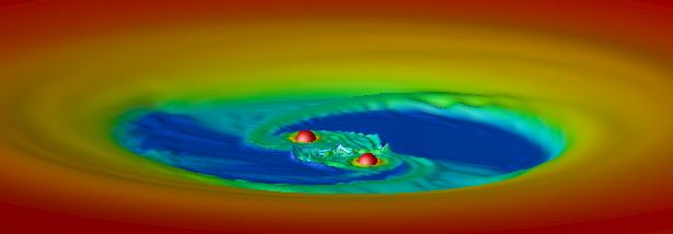
Figure 29: The structure of a circumbinary disk around a central binary star (indicated by the two red spheres in the middle). Color coded is the surface density of the disk and the vertical extension indicates the thickness (temperature) of the disk. (by Richard Günther, University of Tübingen, based on simulations in 2004A&A...423..559G )

Coming back to the evolution of planets embedded in disks we note that Saturn mass planets open a partial gap in the disk. Hence, the corotation torques are reduced and they are driven primarily by the Lindblad torques that will induce inward migration. This inward drift can be stopped at special locations, the so-called planet traps 2006ApJ...642..478M , where the total torque acting on the planet vanishes, such that the inward migration is terminated. Regions with a positive density slope near the inner edge of the disk which will act as a natural location for a planet trap. For single stars a positive density gradient can be generated for example by the magnetosphere of the young star while for binary stars the inner disk cavity is generated naturally by angular momentum transferal from the binary to the disk (see Fig. 29). The extent of the hole, i.e. the location of the disk’s inner edge will then determine the final location of the planet. For typical disk parameter with $\alpha\approx 0.01$, $H/r\approx 0.05$ and binaries with moderate eccentricity, $e_{\rm bin}\approx 0.1$, such as Kepler-16 and Kepler-38 (see table 1) it was shown that in the simulations the final parking position of planets is indeed near the the observed locations 2013A&A...556A.134P ; 2014A&A...564A..72K . In some simulations for Kepler 38 it was found that the planet was captured in the 5:1 resonance and remained at this location. This capture into resonance was accompanied by an increase of the eccentricity of the planetary orbit to about $e_{\rm bin}\approx 0.2$ 2014A&A...564A..72K . As explained above, planets in such resonant orbits will typically be unstable in the longterm evolution and they can only be stable in the presence of a disk that tends to damp planetary eccentricities as shown in the previous section. So, after disk dispersal such a planet is expected to become unstable and be scattered out of the system. It is possible that several planets that initially formed in circumbinary disks experienced such a fate and are now a member of the free-floating planet population. In this case we are just observing those planets that luckily happened to end up in a final stable location in between the unstable resonances. As was shown, different disk parameter with a lower density and viscosity can lead to final parking positions near the observed location for the Kepler-38 system 2014A&A...564A..72K . In Fig. 30 the final parking position is indicated by the innermost orange dot. It is right at the inner edge of the disk.

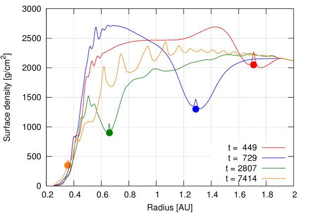
Figure 30: The migration of a planet in the Kepler-38 system. Shown is the surface density at different times (in yrs) after insertion of the planet. The time levels are indicated by the labels. The dots indicate the radial position of the planet at those times, for illustration they have been moved to the corresponding surface density distribution. Clearly visible is the (partial) gap formed by the planet during its inward migration. The orange dot marks the final equilibrium position. Adapted from 2014A&A...564A..72K .

While the final position of planets of planets around binaries with moderate eccentricities (Kepler-16, Kepler-35 and Kepler-38) can be understood in terms of a migration process of a planet in a disk 2013A&A...556A.134P ; 2014A&A...564A..72K , it is still difficult to explain the location of the observed planet in the Kepler-34 systems where the central binary has as large eccentricity of $e_{\rm bin}=0.52$. This high eccentricity of the binary generates a large inner hole of the disk that is highly eccentric and precesses around the central binary with a period of about 120 yrs equivalent to nearly $2000\,P_{\rm bin}$. The final position of the binary is determined by the size of the inner hole. The planet settles in an elliptic orbit that precesses around the binary with exactly the same period as the disk, such that the pericenters of the disk and planet are always aligned. This final orbit has a semi-major axis that is substantially larger than the observed value indicated in Table 1. Hence, for the eccentric binary star Kepler-34, the observed position of the planet is still difficult to understand with a migration process but may be that better disk models with more realistic physics will lead to improved results.

In planetary systems with multiple objects interesting dynamics can take place. Disk-planet interaction will often lead to a convergence of orbits with capture in mean-motion resonances (MMR) between two adjacent planets. However, observationally there is only a slight overabundance of planets near the 3:2 and 2:1 MMRs, but stochastic and tidal processes can take planets out of exact resonance. The dynamical interaction between multiple massive planets can lead to eccentricity and inclination excitation. Another pathway to generate the high observed eccentricity and inclinations in some systems is through the Kozai-Lidov mechanism which requires the exchange of angular momentum with a third, distant object in the system. Concerning the observed abundance of planetary systems that contain several Super-Earths in a compact configuration, the most likely pathway appears to be the convergent inward migration process accompanied by stochastic forces with the disk. A very exciting discovery of the Kepler space mission has been the detection of circumbinary planets. The observed locations of the planets close to the dynamical stability region can be explained for most systems through a migration process of these planets through the circumplanetary disk.

- (1) S. J. Aarseth, From NBODY1 to NBODY6: The Growth of an Industry, PASP, 111 (1999), pp. 1333--1346.
- (2) F. C. Adams and G. Laughlin, Migration and dynamical relaxation in crowded systems of giant planets, Icarus, 163 (2003), pp. 290--306.
- (3) F. C. Adams, G. Laughlin, and A. M. Bloch, Turbulence Implies that Mean Motion Resonances are Rare, ApJ, 683 (2008), pp. 1117--1128.
- (4) ALMA Partnership, C. L. Brogan, L. M. Pérez, T. R. Hunter, W. R. F. Dent, A. S. Hales, R. E. Hills, S. Corder, E. B. Fomalont, C. Vlahakis, Y. Asaki, D. Barkats, A. Hirota, J. A. Hodge, C. M. V. Impellizzeri, R. Kneissl, E. Liuzzo, R. Lucas, N. Marcelino, S. Matsushita, K. Nakanishi, N. Phillips, A. M. S. Richards, I. Toledo, R. Aladro, D. Broguiere, J. R. Cortes, P. C. Cortes, D. Espada, F. Galarza, D. Garcia-Appadoo, L. Guzman-Ramirez, E. M. Humphreys, T. Jung, S. Kameno, R. A. Laing, S. Leon, G. Marconi, A. Mignano, B. Nikolic, L.-A. Nyman, M. Radiszcz, A. Remijan, J. A. Rodón, T. Sawada, S. Takahashi, R. P. J. Tilanus, B. Vila Vilaro, L. C. Watson, T. Wiklind, E. Akiyama, E. Chapillon, I. de Gregorio-Monsalvo, J. Di Francesco, F. Gueth, A. Kawamura, C.-F. Lee, Q. Nguyen Luong, J. Mangum, V. Pietu, P. Sanhueza, K. Saigo, S. Takakuwa, C. Ubach, T. van Kempen, A. Wootten, A. Castro-Carrizo, H. Francke, J. Gallardo, J. Garcia, S. Gonzalez, T. Hill, T. Kaminski, Y. Kurono, H.-Y. Liu, C. Lopez, F. Morales, K. Plarre, G. Schieven, L. Testi, L. Videla, E. Villard, P. Andreani, J. E. Hibbard, and K. Tatematsu, The 2014 ALMA Long Baseline Campaign: First Results from High Angular Resolution Observations toward the HL Tau Region, ApJ, 808 (2015), p. L3.
- (5) S. M. Andrews and J. P. Williams, High-Resolution Submillimeter Constraints on Circumstellar Disk Structure, ApJ, 659 (2007), pp. 705--728.
- (6) P. J. Armitage, Astrophysics of Planet Formation, 2010.
- (7) P. Artymowicz, On the Wave Excitation and a Generalized Torque Formula for Lindblad Resonances Excited by External Potential, ApJ, 419 (1993), p. 155.
- (8) , Dynamics of Gaseous Disks with Planets, in Debris Disks and the Formation of Planets, L. Caroff, L. J. Moon, D. Backman, and E. Praton, eds., vol. 324 of Astronomical Society of the Pacific Conference Series, Dec. 2004, p. 39.
- (9) , Migration Type III, in KITP Conference: Planet Formation: Terrestrial and Extra Solar, Mar. 2004.
- (10) P. Artymowicz and S. H. Lubow, Dynamics of binary-disk interaction. 1: Resonances and disk gap sizes, ApJ, 421 (1994), pp. 651--667.
- (11) S. A. Balbus and J. F. Hawley, A powerful local shear instability in weakly magnetized disks. I - Linear analysis. II - Nonlinear evolution, ApJ, 376 (1991), pp. 214--233.
- (12) N. J. Balmforth and D. G. Korycansky, Non-linear dynamics of the corotation torque, MNRAS, 326 (2001), pp. 833--851.
- (13) I. Baraffe, G. Chabrier, J. Fortney, and C. Sotin, Planetary Internal Structures, Protostars and Planets VI, (2014), pp. 763--786.
- (14) A. J. Barker and G. I. Ogilvie, On the tidal evolution of Hot Jupiters on inclined orbits, MNRAS, 395 (2009), pp. 2268--2287.
- (15) C. Baruteau, A. Crida, S.-J. Paardekooper, F. Masset, J. Guilet, B. Bitsch, R. Nelson, W. Kley, and J. Papaloizou, Planet-Disk Interactions and Early Evolution of Planetary Systems, Protostars and Planets VI, (2014), pp. 667--689.
- (16) C. Baruteau, S. Fromang, R. P. Nelson, and F. Masset, Corotation torques experienced by planets embedded in weakly magnetized turbulent discs, A&A, 533 (2011), p. A84.
- (17) C. Baruteau and D. N. C. Lin, Protoplanetary Migration in Turbulent Isothermal Disks, ApJ, 709 (2010), pp. 759--773.
- (18) C. Baruteau and F. Masset, On the Corotation Torque in a Radiatively Inefficient Disk, ApJ, 672 (2008), pp. 1054--1067.
- (19) , Type I Planetary Migration in a Self-Gravitating Disk, ApJ, 678 (2008), pp. 483--497.
- (20) , Recent Developments in Planet Migration Theory, in Lecture Notes in Physics, Berlin Springer Verlag, J. Souchay, S. Mathis, and T. Tokieda, eds., vol. 861 of Lecture Notes in Physics, Berlin Springer Verlag, 2013, p. 201.
- (21) C. Baruteau, F. Meru, and S.-J. Paardekooper, Rapid inward migration of planets formed by gravitational instability, MNRAS, 416 (2011), pp. 1971--1982.
- (22) K. Batygin and A. Morbidelli, Dissipative Divergence of Resonant Orbits, AJ, 145 (2013), p. 1.
- (23) C. Beaugé, S. Ferraz-Mello, and T. A. Michtchenko, Extrasolar Planets in Mean-Motion Resonance: Apses Alignment and Asymmetric Stationary Solutions, ApJ, 593 (2003), pp. 1124--1133.
- (24) P. Benítez-Llambay, F. Masset, G. Koenigsberger, and J. Szulágyi, Planet heating prevents inward migration of planetary cores, Nature, 520 (2015), pp. 63--65.
- (25) W. Benz, A. Anic, J. Horner, and J. A. Whitby, The Origin of Mercury, Space Sci. Rev., 132 (2007), pp. 189--202.
- (26) W. Benz and E. Asphaug, Impact simulations with fracture. I - Method and tests, Icarus, 107 (1994), p. 98.
- (27) , Catastrophic Disruptions Revisited, Icarus, 142 (1999), pp. 5--20.
- (28) W. Benz, W. L. Slattery, and A. G. W. Cameron, The origin of the moon and the single-impact hypothesis. I, Icarus, 66 (1986), pp. 515--535.
- (29) J. Binney and S. Tremaine, Galactic dynamics, 1987.
- (30) B. Bitsch, A. Crida, A.-S. Libert, and E. Lega, Highly inclined and eccentric massive planets. I. Planet-disc interactions, A&A, 555 (2013), p. A124.
- (31) B. Bitsch, A. Johansen, M. Lambrechts, and A. Morbidelli, The structure of protoplanetary discs around evolving young stars, A&A, 575 (2015), p. A28.
- (32) B. Bitsch and W. Kley, Orbital evolution of eccentric planets in radiative discs, A&A, 523 (2010), p. A30.
- (33) , Evolution of inclined planets in three-dimensional radiative discs, A&A, 530 (2011), p. A41.
- (34) , Range of outward migration and influence of the disc’s mass on the migration of giant planet cores, A&A, 536 (2011), p. A77.
- (35) J. Blum and G. Wurm, The Growth Mechanisms of Macroscopic Bodies in Protoplanetary Disks, ARA&A, 46 (2008), pp. 21--56.
- (36) J. Blum, G. Wurm, S. Kempf, T. Poppe, H. Klahr, T. Kozasa, M. Rott, T. Henning, J. Dorschner, R. Schräpler, H. U. Keller, W. J. Markiewicz, I. Mann, B. A. Gustafson, F. Giovane, D. Neuhaus, H. Fechtig, E. Grün, B. Feuerbacher, H. Kochan, L. Ratke, A. El Goresy, G. Morfill, S. J. Weidenschilling, G. Schwehm, K. Metzler, and W.-H. Ip, Growth and Form of Planetary Seedlings: Results from a Microgravity Aggregation Experiment, Physical Review Letters, 85 (2000), p. 2426.
- (37) P. Bodenheimer, O. Hubickyj, and J. J. Lissauer, Models of the in Situ Formation of Detected Extrasolar Giant Planets,, Icarus, 143 (2000), pp. 2--14.
- (38) P. Bodenheimer and J. B. Pollack, Calculations of the accretion and evolution of giant planets The effects of solid cores, Icarus, 67 (1986), pp. 391--408.
- (39) A. C. Boley, The Two Modes of Gas Giant Planet Formation, ApJ, 695 (2009), pp. L53--L57.
- (40) A. P. Boss, Giant planet formation by gravitational instability., Science, 276 (1997), pp. 1836--1839.
- (41) C. J. Burke, S. T. Bryson, F. Mullally, J. F. Rowe, J. L. Christiansen, S. E. Thompson, J. L. Coughlin, M. R. Haas, N. M. Batalha, D. A. Caldwell, J. M. Jenkins, M. Still, T. Barclay, W. J. Borucki, W. J. Chaplin, D. R. Ciardi, B. D. Clarke, W. D. Cochran, B.-O. Demory, G. A. Esquerdo, T. N. Gautier, III, R. L. Gilliland, F. R. Girouard, M. Havel, C. E. Henze, S. B. Howell, D. Huber, D. W. Latham, J. Li, R. C. Morehead, T. D. Morton, J. Pepper, E. Quintana, D. Ragozzine, S. E. Seader, Y. Shah, A. Shporer, P. Tenenbaum, J. D. Twicken, and A. Wolfgang, Planetary Candidates Observed by Kepler IV: Planet Sample from Q1-Q8 (22 Months), ApJS, 210 (2014), p. 19.
- (42) A. G. W. Cameron, Physics of the primitive solar accretion disk, Moon and Planets, 18 (1978), pp. 5--40.
- (43) P. Cassen, Protostellar Disks and Planet Formation, in Saas-Fee Advanced Course 31: Extrasolar planets, D. Queloz, S. Udry, M. Mayor, W. Benz, P. Cassen, T. Guillot, and A. Quirrenbach, eds., 2006, pp. 369--448.
- (44) G. Chabrier, A. Johansen, M. Janson, and R. Rafikov, Giant Planet and Brown Dwarf Formation, Protostars and Planets VI, (2014), pp. 619--642.
- (45) J. E. Chambers, A hybrid symplectic integrator that permits close encounters between massive bodies, MNRAS, 304 (1999), pp. 793--799.
- (46) , Making More Terrestrial Planets, Icarus, 152 (2001), pp. 205--224.
- (47) , Planetary accretion in the inner Solar System, Earth and Planetary Science Letters, 223 (2004), pp. 241--252.
- (48) J. E. Chambers and G. W. Wetherill, Making the Terrestrial Planets: N-Body Integrations of Planetary Embryos in Three Dimensions, Icarus, 136 (1998), pp. 304--327.
- (49) S. Chatterjee and E. B. Ford, Planetesimal Interactions Can Explain the Mysterious Period Ratios of Small Near-Resonant Planets, ApJ, 803 (2015), p. 33.
- (50) C. E. Chavez, N. Georgakarakos, S. Prodan, M. Reyes-Ruiz, H. Aceves, F. Betancourt, and E. Perez-Tijerina, A dynamical stability study of Kepler Circumbinary planetary systems with one planet, MNRAS, 446 (2015), pp. 1283--1292.
- (51) E. Chiang and G. Laughlin, The minimum-mass extrasolar nebula: in situ formation of close-in super-Earths, MNRAS, 431 (2013), pp. 3444--3455.
- (52) E. Chiang and A. N. Youdin, Forming Planetesimals in Solar and Extrasolar Nebulae, Annual Review of Earth and Planetary Sciences, 38 (2010), pp. 493--522.
- (53) E. I. Chiang and P. Goldreich, Spectral Energy Distributions of T Tauri Stars with Passive Circumstellar Disks, ApJ, 490 (1997), pp. 368--376.
- (54) W. D. Cochran, A. P. Hatzes, R. P. Butler, and G. W. Marcy, The Discovery of a Planetary Companion to 16 Cygni B, ApJ, 483 (1997), pp. 457--463.
- (55) C. Cossou, S. N. Raymond, F. Hersant, and A. Pierens, Hot super-Earths and giant planet cores from different migration histories, A&A, 569 (2014), p. A56.
- (56) P. Cresswell, G. Dirksen, W. Kley, and R. P. Nelson, On the evolution of eccentric and inclined protoplanets embedded in protoplanetary disks, A&A, 473 (2007), pp. 329--342.
- (57) A. Crida and K. Batygin, Spin-orbit angle distribution and the origin of (mis)aligned hot Jupiters, A&A, 567 (2014), p. A42.
- (58) A. Crida, A. Morbidelli, and F. Masset, On the width and shape of gaps in protoplanetary disks, Icarus, 181 (2006), pp. 587--604.
- (59) A. Crida, Z. Sándor, and W. Kley, Influence of an inner disc on the orbital evolution of massive planets migrating in resonance, A&A, 483 (2008), pp. 325--337.
- (60) G. D’Angelo, W. Kley, and T. Henning, Orbital Migration and Mass Accretion of Protoplanets in Three-dimensional Global Computations with Nested Grids, ApJ, 586 (2003), pp. 540--561.
- (61) G. D’Angelo and S. H. Lubow, Three-dimensional Disk-Planet Torques in a Locally Isothermal Disk, ApJ, 724 (2010), pp. 730--747.
- (62) G. D’Angelo, S. H. Lubow, and M. R. Bate, Evolution of Giant Planets in Eccentric Disks, ApJ, 652 (2006), pp. 1698--1714.
- (63) B.-O. Demory and S. Seager, Lack of Inflated Radii for Kepler Giant Planet Candidates Receiving Modest Stellar Irradiation, ApJS, 197 (2011), p. 12.
- (64) S. J. Desch, Mass Distribution and Planet Formation in the Solar Nebula, ApJ, 671 (2007), pp. 878--893.
- (65) M. Desort, A.-M. Lagrange, F. Galland, H. Beust, S. Udry, M. Mayor, and G. Lo Curto, Extrasolar planets and brown dwarfs around A-F type stars. V. A planetary system found with HARPS around the F6IV-V star HD 60532, A&A, 491 (2008), pp. 883--888.
- (66) S. E. Dodson-Robinson, D. Veras, E. B. Ford, and C. A. Beichman, The Formation Mechanism of Gas Giants on Wide Orbits, ApJ, 707 (2009), pp. 79--88.
- (67) C. Dominik and A. G. G. M. Tielens, Resistance to rolling in the adhesive contact of two elastic spheres, Philosophical Magazine, Part A, 72 (1995), pp. 783--803.
- (68) , The Physics of Dust Coagulation and the Structure of Dust Aggregates in Space, ApJ, 480 (1997), pp. 647--673.
- (69) L. R. Doyle, J. A. Carter, D. C. Fabrycky, R. W. Slawson, S. B. Howell, J. N. Winn, J. A. Orosz, A. Prša, W. F. Welsh, S. N. Quinn, D. Latham, G. Torres, L. A. Buchhave, G. W. Marcy, J. J. Fortney, A. Shporer, E. B. Ford, J. J. Lissauer, D. Ragozzine, M. Rucker, N. Batalha, J. M. Jenkins, W. J. Borucki, D. Koch, C. K. Middour, J. R. Hall, S. McCauliff, M. N. Fanelli, E. V. Quintana, M. J. Holman, D. A. Caldwell, M. Still, R. P. Stefanik, W. R. Brown, G. A. Esquerdo, S. Tang, G. Furesz, J. C. Geary, P. Berlind, M. L. Calkins, D. R. Short, J. H. Steffen, D. Sasselov, E. W. Dunham, W. D. Cochran, A. Boss, M. R. Haas, D. Buzasi, and D. Fischer, Kepler-16: A Transiting Circumbinary Planet, Science, 333 (2011), p. 1602.
- (70) B. T. Draine, Interstellar Dust Grains, ARA&A, 41 (2003), pp. 241--289.
- (71) L. Dubrovinsky, N. Dubrovinskaia, V. B. Prakapenka, and A. M. Abakumov, Implementation of micro-ball nanodiamond anvils for high-pressure studies above 6Mbar, Nature Communications, 3 (2012), p. 1163.
- (72) P. C. Duffell, A Simple Analytical Model for Gaps in Protoplanetary Disks, ApJ, 807 (2015), p. L11.
- (73) P. C. Duffell and E. Chiang, Eccentric Jupiters via Disk-Planet Interactions, ApJ, 812 (2015), p. 94.
- (74) P. C. Duffell, Z. Haiman, A. I. MacFadyen, D. J. D’Orazio, and B. D. Farris, The Migration of Gap-opening Planets is Not Locked to Viscous Disk Evolution, ApJ, 792 (2014), p. L10.
- (75) P. C. Duffell and A. I. MacFadyen, Gap Opening by Extremely Low-mass Planets in a Viscous Disk, ApJ, 769 (2013), p. 41.
- (76) M. J. Duncan, H. F. Levison, and M. H. Lee, A Multiple Time Step Symplectic Algorithm for Integrating Close Encounters, AJ, 116 (1998), pp. 2067--2077.
- (77) A. C. Dunhill, R. D. Alexander, and P. J. Armitage, A limit on eccentricity growth from global 3D simulations of disc-planet interactions, MNRAS, 428 (2013), pp. 3072--3082.
- (78) A. C. Dunhill, J. Cuadra, and C. Dougados, Precession and accretion in circumbinary discs: the case of HD 104237, MNRAS, 448 (2015), pp. 3545--3554.
- (79) R. H. Durisen, A. P. Boss, L. Mayer, A. F. Nelson, T. Quinn, and W. K. M. Rice, Gravitational Instabilities in Gaseous Protoplanetary Disks and Implications for Giant Planet Formation, Protostars and Planets V, (2007), pp. 607--622.
- (80) C. Dürmann and W. Kley, Migration of massive planets in accreting disks, A&A, 574 (2015), p. A52.
- (81) R. Dvorak, C. Froeschle, and C. Froeschle, Stability of outer planetary orbits (P-types) in binaries, A&A, 226 (1989), pp. 335--342.
- (82) R. G. Edgar, Giant Planet Migration in Viscous Power-Law Disks, ApJ, 663 (2007), pp. 1325--1334.
- (83) D. Fabrycky and S. Tremaine, Shrinking Binary and Planetary Orbits by Kozai Cycles with Tidal Friction, ApJ, 669 (2007), pp. 1298--1315.
- (84) D. C. Fabrycky and R. A. Murray-Clay, Stability of the Directly Imaged Multiplanet System HR 8799: Resonance and Masses, ApJ, 710 (2010), pp. 1408--1421.
- (85) H. Fahr and E. A. Willerding, Die Entstehung von Sonnensystemen, Spektrum Akademischer Verlag, 1998.
- (86) E. B. Ford and F. A. Rasio, Origins of Eccentric Extrasolar Planets: Testing the Planet-Planet Scattering Model, ApJ, 686 (2008), pp. 621--636.
- (87) J. J. Fortney and N. Nettelmann, The Interior Structure, Composition, and Evolution of Giant Planets, Space Sci. Rev., 152 (2010), pp. 423--447.
- (88) J. Fung, P. Artymowicz, and Y. Wu, The 3D Flow Field Around an Embedded Planet, ApJ, 811 (2015), p. 101.
- (89) J. Fung, J.-M. Shi, and E. Chiang, How Empty are Disk Gaps Opened by Giant Planets?, ApJ, 782 (2014), p. 88.
- (90) C. F. Gammie, Nonlinear Outcome of Gravitational Instability in Cooling, Gaseous Disks, ApJ, 553 (2001), pp. 174--183.
- (91) P. Garaud, F. Meru, M. Galvagni, and C. Olczak, From Dust to Planetesimals: An Improved Model for Collisional Growth in Protoplanetary Disks, ApJ, 764 (2013), p. 146.
- (92) R. J. Geretshauser, F. Meru, R. Speith, and W. Kley, The four-population model: a new classification scheme for pre-planetesimal collisions, A&A, 531 (2011), p. A166.
- (93) P. Goldreich, Y. Lithwick, and R. Sari, Planet Formation by Coagulation: A Focus on Uranus and Neptune, ARA&A, 42 (2004), pp. 549--601.
- (94) P. Goldreich and R. Sari, Eccentricity Evolution for Planets in Gaseous Disks, ApJ, 585 (2003), pp. 1024--1037.
- (95) P. Goldreich and S. Tremaine, The excitation of density waves at the Lindblad and corotation resonances by an external potential, ApJ, 233 (1979), pp. 857--871.
- (96) , Disk-satellite interactions, ApJ, 241 (1980), pp. 425--441.
- (97) P. Goldreich and W. R. Ward, The Formation of Planetesimals, ApJ, 183 (1973), pp. 1051--1062.
- (98) K. Goździewski and C. Migaszewski, Multiple mean motion resonances in the HR 8799 planetary system, MNRAS, 440 (2014), pp. 3140--3171.
- (99) K. Goździewski, C. Migaszewski, F. Panichi, and E. Szuszkiewicz, The Laplace resonance in the Kepler-60 planetary system, MNRAS, 455 (2016), pp. L104--L108.
- (100) Y. Greenzweig and J. J. Lissauer, Accretion rates of protoplanets, Icarus, 87 (1990), pp. 40--77.
- (101) T. Guillot, THE INTERIORS OF GIANT PLANETS: Models and Outstanding Questions, Annual Review of Earth and Planetary Sciences, 33 (2005), pp. 493--530.
- (102) T. Guillot and D. Gautier, Giant Planets, ArXiv e-prints, (2014).
- (103) R. Günther, C. Schäfer, and W. Kley, Evolution of irradiated circumbinary disks, A&A, 423 (2004), pp. 559--566.
- (104) C. Güttler, J. Blum, A. Zsom, C. W. Ormel, and C. P. Dullemond, The outcome of protoplanetary dust growth: pebbles, boulders, or planetesimals?. I. Mapping the zoo of laboratory collision experiments, A&A, 513 (2010), p. A56.
- (105) C. Güttler, M. Krause, R. J. Geretshauser, R. Speith, and J. Blum, The Physics of Protoplanetesimal Dust Agglomerates. IV. Toward a Dynamical Collision Model, ApJ, 701 (2009), pp. 130--141.
- (106) N. Haghighipour, The Formation and Dynamics of Super-Earth Planets, Annual Review of Earth and Planetary Sciences, 41 (2013), pp. 469--495.
- (107) J. Hamel, Geschichte der Astronomie. Von den Anfängen bis zur Gegenwart., 1998.
- (108) B. M. S. Hansen and N. Murray, Migration Then Assembly: Formation of Neptune-mass Planets inside 1 AU, ApJ, 751 (2012), p. 158.
- (109) J. F. Hawley and S. A. Balbus, A Powerful Local Shear Instability in Weakly Magnetized Disks. II. Nonlinear Evolution, ApJ, 376 (1991), p. 223.
- (110) C. Hayashi, Structure of the Solar Nebula, Growth and Decay of Magnetic Fields and Effects of Magnetic and Turbulent Viscosities on the Nebula, Progress of Theoretical Physics Supplement, 70 (1981), pp. 35--53.
- (111) W. Hayes and S. Tremaine, Fitting Selected Random Planetary Systems to Titius-Bode Laws, Icarus, 135 (1998), pp. 549--557.
- (112) D. Heißelmann, J. Blum, H. J. Fraser, and K. Wolling, Microgravity experiments on the collisional behavior of saturnian ring particles, Icarus, 206 (2010), pp. 424--430.
- (113) R. Helled, P. Bodenheimer, M. Podolak, A. Boley, F. Meru, S. Nayakshin, J. J. Fortney, L. Mayer, Y. Alibert, and A. P. Boss, Giant Planet Formation, Evolution, and Internal Structure, Protostars and Planets VI, (2014), pp. 643--665.
- (114) H. Hertz, über die Berührung fester elastischer Körper, J. reine und angewandte Mathematik, 94 (1882), pp. 156--171.
- (115) M. Holman, J. Touma, and S. Tremaine, Chaotic variations in the eccentricity of the planet orbiting 16 Cygni B, Nature, 386 (1997), pp. 254--256.
- (116) M. J. Holman and P. A. Wiegert, Long-Term Stability of Planets in Binary Systems, AJ, 117 (1999), pp. 621--628.
- (117) P. B. Ivanov, J. C. B. Papaloizou, and A. G. Polnarev, The evolution of a supermassive binary caused by an accretion disc, MNRAS, 307 (1999), pp. 79--90.
- (118) T. Jankowski, G. Wurm, T. Kelling, J. Teiser, W. Sabolo, P. J. Gutiérrez, and I. Bertini, Crossing barriers in planetesimal formation: The growth of mm-dust aggregates with large constituent grains, A&A, 542 (2012), p. A80.
- (119) A. Johansen, J. Blum, H. Tanaka, C. Ormel, M. Bizzarro, and H. Rickman, The Multifaceted Planetesimal Formation Process, Protostars and Planets VI, (2014), pp. 547--570.
- (120) A. Johansen, J. S. Oishi, M.-M. Mac Low, H. Klahr, T. Henning, and A. Youdin, Rapid planetesimal formation in turbulent circumstellar disks, Nature, 448 (2007), pp. 1022--1025.
- (121) K. L. Johnson, K. Kendall, and A. D. Roberts, Surface Energy and the Contact of Elastic Solids, Royal Society of London Proceedings Series A, 324 (1971), pp. 301--313.
- (122) M. Jurić and S. Tremaine, Dynamical Origin of Extrasolar Planet Eccentricity Distribution, ApJ, 686 (2008), pp. 603--620.
- (123) K. D. Kanagawa, T. Muto, H. Tanaka, T. Tanigawa, T. Takeuchi, T. Tsukagoshi, and M. Momose, Mass Estimates of a Giant Planet in a Protoplanetary Disk from the Gap Structures, ApJ, 806 (2015), p. L15.
- (124) I. Kant, Allgemeine Naturgeschichte und Theorie des Himmels, 1755.
- (125) R. Kippenhahn and A. Weigert, Stellar Structure and Evolution, 1990.
- (126) W. Kley, Mass flow and accretion through gaps in accretion discs, MNRAS, 303 (1999), pp. 696--710.
- (127) W. Kley, B. Bitsch, and H. Klahr, Planet migration in three-dimensional radiative discs, A&A, 506 (2009), pp. 971--987.
- (128) W. Kley and A. Crida, Migration of protoplanets in radiative discs, A&A, 487 (2008), pp. L9--L12.
- (129) W. Kley and G. Dirksen, Disk eccentricity and embedded planets, A&A, 447 (2006), pp. 369--377.
- (130) W. Kley and N. Haghighipour, Modeling circumbinary planets: The case of Kepler-38, A&A, 564 (2014), p. A72.
- (131) , Evolution of circumbinary planets around eccentric binaries: The case of Kepler-34, A&A, 581 (2015), p. A20.
- (132) W. Kley, T. W. A. Müller, S. M. Kolb, P. Benítez-Llambay, and F. Masset, Low-mass planets in nearly inviscid disks: numerical treatment, A&A, 546 (2012), p. A99.
- (133) W. Kley and R. P. Nelson, Planet-Disk Interaction and Orbital Evolution, ARA&A, 50 (2012), pp. 211--249.
- (134) W. Kley, J. Peitz, and G. Bryden, Evolution of planetary systems in resonance, A&A, 414 (2004), pp. 735--747.
- (135) E. Kokubo, Planetary Accretion: From Planitesimals to Protoplanets, in Reviews in Modern Astronomy, R. E. Schielicke, ed., vol. 14 of Reviews in Modern Astronomy, 2001, p. 117.
- (136) E. Kokubo and S. Ida, Oligarchic Growth of Protoplanets, Icarus, 131 (1998), pp. 171--178.
- (137) , Formation of Protoplanet Systems and Diversity of Planetary Systems, ApJ, 581 (2002), pp. 666--680.
- (138) J. Kominami and S. Ida, The Effect of Tidal Interaction with a Gas Disk on Formation of Terrestrial Planets, Icarus, 157 (2002), pp. 43--56.
- (139) Y. Kozai, Secular perturbations of asteroids with high inclination and eccentricity, AJ, 67 (1962), p. 591.
- (140) K. M. Kratter, R. A. Murray-Clay, and A. N. Youdin, The Runts of the Litter: Why Planets Formed Through Gravitational Instability Can Only Be Failed Binary Stars, ApJ, 710 (2010), pp. 1375--1386.
- (141) M. Krause and J. Blum, Growth and Form of Planetary Seedlings: Results from a Sounding Rocket Microgravity Aggregation Experiment, Physical Review Letters, 93 (2004), p. 021103.
- (142) K. A. Kretke and D. N. C. Lin, Grain Retention and Formation of Planetesimals near the Snow Line in MRI-driven Turbulent Protoplanetary Disks, ApJ, 664 (2007), pp. L55--L58.
- (143) G. P. Kuiper, On the Origin of the Solar System, Proceedings of the National Academy of Science, 37 (1951), pp. 1--14.
- (144) M. Lambrechts and A. Johansen, Rapid growth of gas-giant cores by pebble accretion, A&A, 544 (2012), p. A32.
- (145) P.-S. Laplace, Exposition du système du monde, 1776.
- (146) G. Laughlin, V. Korchagin, and F. C. Adams, The Dynamics of Heavy Gaseous Disks, ApJ, 504 (1998), pp. 945--966.
- (147) G. Laughlin, A. Steinacker, and F. C. Adams, Type I Planetary Migration with MHD Turbulence, ApJ, 608 (2004), pp. 489--496.
- (148) M. H. Lee and S. J. Peale, Dynamics and Origin of the 2:1 Orbital Resonances of the GJ 876 Planets, ApJ, 567 (2002), pp. 596--609.
- (149) E. Lega, A. Crida, B. Bitsch, and A. Morbidelli, Migration of Earth-sized planets in 3D radiative discs, MNRAS, 440 (2014), pp. 683--695.
- (150) Z. M. Leinhardt and D. C. Richardson, N-Body Simulations of Planetesimal Evolution: Effect of Varying Impactor Mass Ratio, Icarus, 159 (2002), pp. 306--313.
- (151) Z. M. Leinhardt, D. C. Richardson, and T. Quinn, Direct N-body Simulations of Rubble Pile Collisions, Icarus, 146 (2000), pp. 133--151.
- (152) Z. M. Leinhardt and S. T. Stewart, Full numerical simulations of catastrophic small body collisions, Icarus, 199 (2009), pp. 542--559.
- (153) H. Li, S. H. Lubow, S. Li, and D. N. C. Lin, Type I Planet Migration in Nearly Laminar Disks, ApJ, 690 (2009), pp. L52--L55.
- (154) C. C. Lin and F. H. Shu, On the Spiral Structure of Disk Galaxies., ApJ, 140 (1964), p. 646.
- (155) D. N. C. Lin, P. Bodenheimer, and D. C. Richardson, Orbital migration of the planetary companion of 51 Pegasi to its present location, Nature, 380 (1996), pp. 606--607.
- (156) D. N. C. Lin and J. Papaloizou, Tidal torques on accretion discs in binary systems with extreme mass ratios, MNRAS, 186 (1979), pp. 799--812.
- (157) , On the tidal interaction between protoplanets and the protoplanetary disk. III - Orbital migration of protoplanets, ApJ, 309 (1986), pp. 846--857.
- (158) J. J. Lissauer, Timescales for planetary accretion and the structure of the protoplanetary disk, Icarus, 69 (1987), pp. 249--265.
- (159) , Planet formation, ARA&A, 31 (1993), pp. 129--174.
- (160) J. J. Lissauer and G. R. Stewart, Growth of planets from planetesimals, in Protostars and Planets III, E. H. Levy and J. I. Lunine, eds., 1993, pp. 1061--1088.
- (161) Y. Lithwick and Y. Wu, Resonant Repulsion of Kepler Planet Pairs, ApJ, 756 (2012), p. L11.
- (162) S. H. Lubow, M. Seibert, and P. Artymowicz, Disk Accretion onto High-Mass Planets, ApJ, 526 (1999), pp. 1001--1012.
- (163) D. Lynden-Bell and J. E. Pringle, The evolution of viscous discs and the origin of the nebular variables., MNRAS, 168 (1974), pp. 603--637.
- (164) M.-M. Mac Low and R. S. Klessen, Control of star formation by supersonic turbulence, Reviews of Modern Physics, 76 (2004), pp. 125--194.
- (165) N. Madhusudhan, K. K. M. Lee, and O. Mousis, A Possible Carbon-rich Interior in Super-Earth 55 Cancri e, ApJ, 759 (2012), p. L40.
- (166) U. Marboeuf, A. Thiabaud, Y. Alibert, N. Cabral, and W. Benz, From planetesimals to planets: volatile molecules, A&A, 570 (2014), p. A36.
- (167) G. W. Marcy, R. P. Butler, D. Fischer, S. S. Vogt, J. J. Lissauer, and E. J. Rivera, A Pair of Resonant Planets Orbiting GJ 876, ApJ, 556 (2001), pp. 296--301.
- (168) G. W. Marcy, H. Isaacson, A. W. Howard, J. F. Rowe, J. M. Jenkins, S. T. Bryson, D. W. Latham, S. B. Howell, T. N. Gautier, III, N. M. Batalha, L. Rogers, D. Ciardi, D. A. Fischer, R. L. Gilliland, H. Kjeldsen, J. Christensen-Dalsgaard, D. Huber, W. J. Chaplin, S. Basu, L. A. Buchhave, S. N. Quinn, W. J. Borucki, D. G. Koch, R. Hunter, D. A. Caldwell, J. Van Cleve, R. Kolbl, L. M. Weiss, E. Petigura, S. Seager, T. Morton, J. A. Johnson, S. Ballard, C. Burke, W. D. Cochran, M. Endl, P. MacQueen, M. E. Everett, J. J. Lissauer, E. B. Ford, G. Torres, F. Fressin, T. M. Brown, J. H. Steffen, D. Charbonneau, G. S. Basri, D. D. Sasselov, J. Winn, R. Sanchis-Ojeda, J. Christiansen, E. Adams, C. Henze, A. Dupree, D. C. Fabrycky, J. J. Fortney, J. Tarter, M. J. Holman, P. Tenenbaum, A. Shporer, P. W. Lucas, W. F. Welsh, J. A. Orosz, T. R. Bedding, T. L. Campante, G. R. Davies, Y. Elsworth, R. Handberg, S. Hekker, C. Karoff, S. D. Kawaler, M. N. Lund, M. Lundkvist, T. S. Metcalfe, A. Miglio, V. Silva Aguirre, D. Stello, T. R. White, A. Boss, E. Devore, A. Gould, A. Prsa, E. Agol, T. Barclay, J. Coughlin, E. Brugamyer, F. Mullally, E. V. Quintana, M. Still, S. E. Thompson, D. Morrison, J. D. Twicken, J.-M. Désert, J. Carter, J. R. Crepp, G. Hébrard, A. Santerne, C. Moutou, C. Sobeck, D. Hudgins, M. R. Haas, P. Robertson, J. Lillo-Box, and D. Barrado, Masses, Radii, and Orbits of Small Kepler Planets: The Transition from Gaseous to Rocky Planets, ApJS, 210 (2014), p. 20.
- (169) C. Marois, B. Macintosh, T. Barman, B. Zuckerman, I. Song, J. Patience, D. Lafrenière, and R. Doyon, Direct Imaging of Multiple Planets Orbiting the Star HR 8799, Science, 322 (2008), p. 1348.
- (170) C. Marois, B. Zuckerman, Q. M. Konopacky, B. Macintosh, and T. Barman, Images of a fourth planet orbiting HR 8799, Nature, 468 (2010), pp. 1080--1083.
- (171) J. G. Martí, C. A. Giuppone, and C. Beaugé, Dynamical analysis of the Gliese-876 Laplace resonance, MNRAS, 433 (2013), pp. 928--934.
- (172) F. Marzari and A. F. Nelson, Interaction of a Giant Planet in an Inclined Orbit with a Circumstellar Disk, ApJ, 705 (2009), pp. 1575--1583.
- (173) F. Marzari, P. Thebault, H. Scholl, G. Picogna, and C. Baruteau, Influence of the circumbinary disk gravity on planetesimal accumulation in the Kepler-16 system, A&A, 553 (2013), p. A71.
- (174) F. Masset, FARGO: A fast eulerian transport algorithm for differentially rotating disks, A&AS, 141 (2000), pp. 165--173.
- (175) F. S. Masset, The co-orbital corotation torque in a viscous disk: Numerical simulations, A&A, 387 (2002), pp. 605--623.
- (176) F. S. Masset and J. Casoli, Saturated Torque Formula for Planetary Migration in Viscous Disks with Thermal Diffusion: Recipe for Protoplanet Population Synthesis, ApJ, 723 (2010), pp. 1393--1417.
- (177) F. S. Masset, A. Morbidelli, A. Crida, and J. Ferreira, Disk Surface Density Transitions as Protoplanet Traps, ApJ, 642 (2006), pp. 478--487.
- (178) F. S. Masset and J. C. B. Papaloizou, Runaway Migration and the Formation of Hot Jupiters, ApJ, 588 (2003), pp. 494--508.
- (179) J. S. Mathis, W. Rumpl, and K. H. Nordsieck, The size distribution of interstellar grains, ApJ, 217 (1977), pp. 425--433.
- (180) L. Mayer, T. Quinn, J. Wadsley, and J. Stadel, Formation of Giant Planets by Fragmentation of Protoplanetary Disks, Science, 298 (2002), pp. 1756--1759.
- (181) , The Evolution of Gravitationally Unstable Protoplanetary Disks: Fragmentation and Possible Giant Planet Formation, ApJ, 609 (2004), pp. 1045--1064.
- (182) M. Mayor and D. Queloz, A Jupiter-mass companion to a solar-type star, Nature, 378 (1995), pp. 355--359.
- (183) M. J. McCaughrean and C. R. O’dell, Direct Imaging of Circumstellar Disks in the Orion Nebula, AJ, 111 (1996), p. 1977.
- (184) A. C. Mejía, R. H. Durisen, M. K. Pickett, and K. Cai, The Thermal Regulation of Gravitational Instabilities in Protoplanetary Disks. II. Extended Simulations with Varied Cooling Rates, ApJ, 619 (2005), pp. 1098--1113.
- (185) F. Meru and M. R. Bate, Non-convergence of the critical cooling time-scale for fragmentation of self-gravitating discs, MNRAS, 411 (2011), pp. L1--L5.
- (186) , On the convergence of the critical cooling time-scale for the fragmentation of self-gravitating discs, MNRAS, 427 (2012), pp. 2022--2046.
- (187) S. Meschiari, Circumbinary Planet Formation in the Kepler-16 System. I. N-body Simulations, ApJ, 752 (2012), p. 71.
- (188) S. Michael, R. H. Durisen, and A. C. Boley, Migration of Gas Giant Planets in Gravitationally Unstable Disks, ApJ, 737 (2011), p. L42.
- (189) S. M. Mills, D. C. Fabrycky, C. Migaszewski, E. B. Ford, E. Petigura, and H. Isaacson, A resonant chain of four transiting, sub-Neptune planets, Nature, 533 (2016), pp. 509--512.
- (190) H. Mizuno, Formation of the Giant Planets, Progress of Theoretical Physics, 64 (1980), pp. 544--557.
- (191) H. Mizuno, K. Nakazawa, and C. Hayashi, Instability of a gaseous envelope surrounding a planetary core and formation of giant planets, Progress of Theoretical Physics, 60 (1978), pp. 699--710.
- (192) J. J. Monaghan, Smoothed particle hydrodynamics, Reports on Progress in Physics, 68 (2005), pp. 1703--1759.
- (193) T. Montmerle, J.-C. Augereau, M. Chaussidon, M. Gounelle, B. Marty, and A. Morbidelli, From Suns to Life: A Chronological Approach to the History of Life on Earth 3. Solar System Formation and Early Evolution: the First 100 Million Years, Earth Moon and Planets, 98 (2006), pp. 39--95.
- (194) A. Morbidelli, J. I. Lunine, D. P. O’Brien, S. N. Raymond, and K. J. Walsh, Building Terrestrial Planets, Annual Review of Earth and Planetary Sciences, 40 (2012), pp. 251--275.
- (195) C. Mordasini, Y. Alibert, H. Klahr, and T. Henning, Characterization of exoplanets from their formation. I. Models of combined planet formation and evolution, A&A, 547 (2012), p. A111.
- (196) C. Mordasini, P. Mollière, K.-M. Dittkrist, S. Jin, and Y. Alibert, Global models of planet formation and evolution, International Journal of Astrobiology, 14 (2015), pp. 201--232.
- (197) T. W. A. Müller, W. Kley, and F. Meru, Treating gravity in thin-disk simulations, A&A, 541 (2012), p. A123.
- (198) C. D. Murray and S. F. Dermott, Solar system dynamics, 1999.
- (199) S. Nayakshin, Formation of planets by tidal downsizing of giant planet embryos, MNRAS, 408 (2010), pp. L36--L40.
- (200) R. P. Nelson, On the orbital evolution of low mass protoplanets in turbulent, magnetised disks, A&A, 443 (2005), pp. 1067--1085.
- (201) R. P. Nelson and J. C. B. Papaloizou, The interaction of giant planets with a disc with MHD turbulence - IV. Migration rates of embedded protoplanets, MNRAS, 350 (2004), pp. 849--864.
- (202) R. P. Nelson, J. C. B. Papaloizou, F. Masset, and W. Kley, The migration and growth of protoplanets in protostellar discs, MNRAS, 318 (2000), pp. 18--36.
- (203) D. P. O’Brien, A. Morbidelli, and H. F. Levison, Terrestrial planet formation with strong dynamical friction, Icarus, 184 (2006), pp. 39--58.
- (204) S.-J. Paardekooper, Numerical convergence in self-gravitating shearing sheet simulations and the stochastic nature of disc fragmentation, MNRAS, 421 (2012), pp. 3286--3299.
- (205) S.-J. Paardekooper, C. Baruteau, A. Crida, and W. Kley, A torque formula for non-isothermal type I planetary migration - I. Unsaturated horseshoe drag, MNRAS, 401 (2010), pp. 1950--1964.
- (206) S.-J. Paardekooper, C. Baruteau, and W. Kley, A torque formula for non-isothermal Type I planetary migration - II. Effects of diffusion, MNRAS, 410 (2011), pp. 293--303.
- (207) S.-J. Paardekooper, Z. M. Leinhardt, P. Thébault, and C. Baruteau, How Not to Build Tatooine: The Difficulty of In Situ Formation of Circumbinary Planets Kepler 16b, Kepler 34b, and Kepler 35b, ApJ, 754 (2012), p. L16.
- (208) S.-J. Paardekooper and G. Mellema, Halting type I planet migration in non-isothermal disks, A&A, 459 (2006), pp. L17--L20.
- (209) S.-J. Paardekooper and J. C. B. Papaloizou, On disc protoplanet interactions in a non-barotropic disc with thermal diffusion, A&A, 485 (2008), pp. 877--895.
- (210) S.-J. Paardekooper, H. Rein, and W. Kley, The formation of systems with closely spaced low-mass planets and the application to Kepler-36, MNRAS, 434 (2013), pp. 3018--3029.
- (211) J. C. B. Papaloizou and J. D. Larwood, On the orbital evolution and growth of protoplanets embedded in a gaseous disc, MNRAS, 315 (2000), pp. 823--833.
- (212) J. C. B. Papaloizou and R. P. Nelson, Models of accreting gas giant protoplanets in protostellar disks, A&A, 433 (2005), pp. 247--265.
- (213) J. C. B. Papaloizou, R. P. Nelson, W. Kley, F. S. Masset, and P. Artymowicz, Disk-Planet Interactions During Planet Formation, Protostars and Planets V, (2007), pp. 655--668.
- (214) J. C. B. Papaloizou, R. P. Nelson, and F. Masset, Orbital eccentricity growth through disc-companion tidal interaction, A&A, 366 (2001), pp. 263--275.
- (215) D. Paszun and C. Dominik, Numerical determination of the material properties of porous dust cakes, A&A, 484 (2008), pp. 859--868.
- (216) A. Pepliński, P. Artymowicz, and G. Mellema, Numerical simulations of type III planetary migration - II. Inward migration of massive planets, MNRAS, 386 (2008), pp. 179--198.
- (217) , Numerical simulations of type III planetary migration - III. Outward migration of massive planets, MNRAS, 387 (2008), pp. 1063--1079.
- (218) F. Perri and A. G. W. Cameron, Hydrodynamic instability of the solar nebula in the presence of a planetary core, Icarus, 22 (1974), pp. 416--425.
- (219) M. Perryman, The Exoplanet Handbook, May 2011.
- (220) E. A. Petigura, A. W. Howard, and G. W. Marcy, Prevalence of Earth-size planets orbiting Sun-like stars, Proceedings of the National Academy of Science, 110 (2013), pp. 19273--19278.
- (221) A. Pierens and J.-M. Huré, How does disk gravity really influence type-I migration?, A&A, 433 (2005), pp. L37--L40.
- (222) A. Pierens and R. P. Nelson, On the migration of protoplanets embedded in circumbinary disks, A&A, 472 (2007), pp. 993--1001.
- (223) , Constraints on resonant-trapping for two planets embedded in a protoplanetary disc, A&A, 482 (2008), pp. 333--340.
- (224) , Migration and gas accretion scenarios for the Kepler 16, 34, and 35 circumbinary planets, A&A, 556 (2013), p. A134.
- (225) J. B. Pollack, O. Hubickyj, P. Bodenheimer, J. J. Lissauer, M. Podolak, and Y. Greenzweig, Formation of the Giant Planets by Concurrent Accretion of Solids and Gas, Icarus, 124 (1996), pp. 62--85.
- (226) T. Poppe, J. Blum, and T. Henning, Analogous Experiments on the Stickiness of Micron-sized Preplanetary Dust, ApJ, 533 (2000), pp. 454--471.
- (227) J. E. Pringle, Accretion discs in astrophysics, ARA&A, 19 (1981), pp. 137--162.
- (228) A. Quirrenbach, Detection and Characterization of Extrasolar Planets, in Saas-Fee Advanced Course 31: Extrasolar planets, D. Queloz, S. Udry, M. Mayor, W. Benz, P. Cassen, T. Guillot, and A. Quirrenbach, eds., 2006, pp. 1--242.
- (229) R. R. Rafikov, Planet Migration and Gap Formation by Tidally Induced Shocks, ApJ, 572 (2002), pp. 566--579.
- (230) , Can Giant Planets Form by Direct Gravitational Instability?, ApJ, 621 (2005), pp. L69--L72.
- (231) H. Rauer, C. Catala, C. Aerts, T. Appourchaux, W. Benz, A. Brandeker, J. Christensen-Dalsgaard, M. Deleuil, L. Gizon, M.-J. Goupil, M. Güdel, E. Janot-Pacheco, M. Mas-Hesse, I. Pagano, G. Piotto, D. Pollacco, Ċ. Santos, A. Smith, J.-C. Suárez, R. Szabó, S. Udry, V. Adibekyan, Y. Alibert, J.-M. Almenara, P. Amaro-Seoane, M. A.-v. Eiff, M. Asplund, E. Antonello, S. Barnes, F. Baudin, K. Belkacem, M. Bergemann, G. Bihain, A. C. Birch, X. Bonfils, I. Boisse, A. S. Bonomo, F. Borsa, I. M. Brandão, E. Brocato, S. Brun, M. Burleigh, R. Burston, J. Cabrera, S. Cassisi, W. Chaplin, S. Charpinet, C. Chiappini, R. P. Church, S. Csizmadia, M. Cunha, M. Damasso, M. B. Davies, H. J. Deeg, R. F. Díaz, S. Dreizler, C. Dreyer, P. Eggenberger, D. Ehrenreich, P. Eigmüller, A. Erikson, R. Farmer, S. Feltzing, F. de Oliveira Fialho, P. Figueira, T. Forveille, M. Fridlund, R. A. García, P. Giommi, G. Giuffrida, M. Godolt, J. Gomes da Silva, T. Granzer, J. L. Grenfell, A. Grotsch-Noels, E. Günther, C. A. Haswell, A. P. Hatzes, G. Hébrard, S. Hekker, R. Helled, K. Heng, J. M. Jenkins, A. Johansen, M. L. Khodachenko, K. G. Kislyakova, W. Kley, U. Kolb, N. Krivova, F. Kupka, H. Lammer, A. F. Lanza, Y. Lebreton, D. Magrin, P. Marcos-Arenal, P. M. Marrese, J. P. Marques, J. Martins, S. Mathis, S. Mathur, S. Messina, A. Miglio, J. Montalban, M. Montalto, M. J. P. F. G. Monteiro, H. Moradi, E. Moravveji, C. Mordasini, T. Morel, A. Mortier, V. Nascimbeni, R. P. Nelson, M. B. Nielsen, L. Noack, A. J. Norton, A. Ofir, M. Oshagh, R.-M. Ouazzani, P. Pápics, V. C. Parro, P. Petit, B. Plez, E. Poretti, A. Quirrenbach, R. Ragazzoni, G. Raimondo, M. Rainer, D. R. Reese, R. Redmer, S. Reffert, B. Rojas-Ayala, I. W. Roxburgh, S. Salmon, A. Santerne, J. Schneider, J. Schou, S. Schuh, H. Schunker, A. Silva-Valio, R. Silvotti, I. Skillen, I. Snellen, F. Sohl, S. G. Sousa, A. Sozzetti, D. Stello, K. G. Strassmeier, M. Švanda, G. M. Szabó, A. Tkachenko, D. Valencia, V. Van Grootel, S. D. Vauclair, P. Ventura, F. W. Wagner, N. A. Walton, J. Weingrill, S. C. Werner, P. J. Wheatley, and K. Zwintz, The PLATO 2.0 mission, Experimental Astronomy, 38 (2014), pp. 249--330.
- (232) S. N. Raymond and C. Cossou, No universal minimum-mass extrasolar nebula: evidence against in situ accretion of systems of hot super-Earths, MNRAS, 440 (2014), pp. L11--L15.
- (233) S. N. Raymond, E. Kokubo, A. Morbidelli, R. Morishima, and K. J. Walsh, Terrestrial Planet Formation at Home and Abroad, Protostars and Planets VI, (2014), pp. 595--618.
- (234) S. N. Raymond, D. P. O’Brien, A. Morbidelli, and N. A. Kaib, Building the terrestrial planets: Constrained accretion in the inner Solar System, Icarus, 203 (2009), pp. 644--662.
- (235) S. N. Raymond, T. Quinn, and J. I. Lunine, Making other earths: dynamical simulations of terrestrial planet formation and water delivery, Icarus, 168 (2004), pp. 1--17.
- (236) , High-resolution simulations of the final assembly of Earth-like planets I. Terrestrial accretion and dynamics, Icarus, 183 (2006), pp. 265--282.
- (237) H. Rein, Period ratios in multiplanetary systems discovered by Kepler are consistent with planet migration, MNRAS, 427 (2012), pp. L21--L24.
- (238) , Planet-disc interaction in highly inclined systems, MNRAS, 422 (2012), pp. 3611--3616.
- (239) H. Rein and S.-F. Liu, REBOUND: an open-source multi-purpose N-body code for collisional dynamics, A&A, 537 (2012), p. A128.
- (240) W. K. M. Rice, P. J. Armitage, M. R. Bate, and I. A. Bonnell, The effect of cooling on the global stability of self-gravitating protoplanetary discs, MNRAS, 339 (2003), pp. 1025--1030.
- (241) W. K. M. Rice, G. Lodato, J. E. Pringle, P. J. Armitage, and I. A. Bonnell, Planetesimal formation via fragmentation in self-gravitating protoplanetary discs, MNRAS, 372 (2006), pp. L9--L13.
- (242) W. K. M. Rice, S.-J. Paardekooper, D. H. Forgan, and P. J. Armitage, Convergence of simulations of self-gravitating accretion discs - II. Sensitivity to the implementation of radiative cooling and artificial viscosity, MNRAS, 438 (2014), pp. 1593--1602.
- (243) G. R. Ricker, J. N. Winn, R. Vanderspek, D. W. Latham, G. Á. Bakos, J. L. Bean, Z. K. Berta-Thompson, T. M. Brown, L. Buchhave, N. R. Butler, R. P. Butler, W. J. Chaplin, D. Charbonneau, J. Christensen-Dalsgaard, M. Clampin, D. Deming, J. Doty, N. De Lee, C. Dressing, E. W. Dunham, M. Endl, F. Fressin, J. Ge, T. Henning, M. J. Holman, A. W. Howard, S. Ida, J. M. Jenkins, G. Jernigan, J. A. Johnson, L. Kaltenegger, N. Kawai, H. Kjeldsen, G. Laughlin, A. M. Levine, D. Lin, J. J. Lissauer, P. MacQueen, G. Marcy, P. R. McCullough, T. D. Morton, N. Narita, M. Paegert, E. Palle, F. Pepe, J. Pepper, A. Quirrenbach, S. A. Rinehart, D. Sasselov, B. Sato, S. Seager, A. Sozzetti, K. G. Stassun, P. Sullivan, A. Szentgyorgyi, G. Torres, S. Udry, and J. Villasenor, Transiting Exoplanet Survey Satellite (TESS), Journal of Astronomical Telescopes, Instruments, and Systems, 1 (2015), p. 014003.
- (244) E. J. Rivera, G. Laughlin, R. P. Butler, S. S. Vogt, N. Haghighipour, and S. Meschiari, The Lick-Carnegie Exoplanet Survey: a Uranus-Mass Fourth Planet for GJ 876 in an Extrasolar Laplace Configuration, ApJ, 719 (2010), pp. 890--899.
- (245) V. S. Safronov, Evolution of the protoplanetary cloud and formation of the earth and planets., 1972.
- (246) Z. Sándor, W. Kley, and P. Klagyivik, Stability and formation of the resonant system HD 73526, A&A, 472 (2007), pp. 981--992.
- (247) D. Saumon and T. Guillot, Shock Compression of Deuterium and the Interiors of Jupiter and Saturn, ApJ, 609 (2004), pp. 1170--1180.
- (248) H. E. Schlichting, C. I. Fuentes, and D. E. Trilling, Initial Planetesimal Sizes and the Size Distribution of Small Kuiper Belt Objects, AJ, 146 (2013), p. 36.
- (249) H. Scholl, F. Marzari, and P. Thébault, Relative velocities among accreting planetesimals in binary systems: the circumbinary case, MNRAS, 380 (2007), pp. 1119--1126.
- (250) A. Seizinger and W. Kley, Bouncing behavior of microscopic dust aggregates, A&A, 551 (2013), p. A65.
- (251) A. Seizinger, R. Speith, and W. Kley, Compression behavior of porous dust agglomerates, A&A, 541 (2012), p. A59.
- (252) Y. Shen and E. L. Turner, On the Eccentricity Distribution of Exoplanets from Radial Velocity Surveys, ApJ, 685 (2008), pp. 553--559.
- (253) F. H. Shu, The physics of astrophysics. Volume II: Gas dynamics., 1992.
- (254) A. Silburt and H. Rein, Tides alone cannot explain Kepler planets close to 2:1 MMR, MNRAS, 453 (2015), pp. 4089--4096.
- (255) D. S. Spiegel and A. Burrows, Spectral and Photometric Diagnostics of Giant Planet Formation Scenarios, ApJ, 745 (2012), p. 174.
- (256) D. J. Stevenson, Formation of the giant planets, Planet. Space Sci., 30 (1982), pp. 755--764.
- (257) S. T. Stewart and Z. M. Leinhardt, Velocity-Dependent Catastrophic Disruption Criteria for Planetesimals, ApJ, 691 (2009), pp. L133--L137.
- (258) D. Syer and C. J. Clarke, Satellites in discs: regulating the accretion luminosity, MNRAS, 277 (1995), pp. 758--766.
- (259) J. Szulágyi, A. Morbidelli, A. Crida, and F. Masset, Accretion of Jupiter-mass Planets in the Limit of Vanishing Viscosity, ApJ, 782 (2014), p. 65.
- (260) H. Tanaka, T. Takeuchi, and W. R. Ward, Three-Dimensional Interaction between a Planet and an Isothermal Gaseous Disk. I. Corotation and Lindblad Torques and Planet Migration, ApJ, 565 (2002), pp. 1257--1274.
- (261) H. Tanaka and W. R. Ward, Three-dimensional Interaction between a Planet and an Isothermal Gaseous Disk. II. Eccentricity Waves and Bending Waves, ApJ, 602 (2004), pp. 388--395.
- (262) E. W. Thommes, M. J. Duncan, and H. F. Levison, Oligarchic growth of giant planets, Icarus, 161 (2003), pp. 431--455.
- (263) A. Toomre, On the gravitational stability of a disk of stars, ApJ, 139 (1964), pp. 1217--1238.
- (264) Y. Tsukamoto, M. N. Machida, and S.-i. Inutsuka, Formation, orbital and thermal evolution, and survival of planetary-mass clumps in the early phase of circumstellar disc evolution, MNRAS, 436 (2013), pp. 1667--1673.
- (265) S. Udry and N. C. Santos, Statistical Properties of Exoplanets, ARA&A, 45 (2007), pp. 397--439.
- (266) A. L. Uribe, H. Klahr, M. Flock, and T. Henning, Three-dimensional Magnetohydrodynamic Simulations of Planet Migration in Turbulent Stratified Disks, ApJ, 736 (2011), p. 85.
- (267) S. S. Vogt, R. P. Butler, G. W. Marcy, D. A. Fischer, G. W. Henry, G. Laughlin, J. T. Wright, and J. A. Johnson, Five New Multicomponent Planetary Systems, ApJ, 632 (2005), pp. 638--658.
- (268) E. I. Vorobyov, Formation of giant planets and brown dwarfs on wide orbits, A&A, 552 (2013), p. A129.
- (269) E. I. Vorobyov and S. Basu, The Burst Mode of Protostellar Accretion, ApJ, 650 (2006), pp. 956--969.
- (270) , Formation and Survivability of Giant Planets on Wide Orbits, ApJ, 714 (2010), pp. L133--L137.
- (271) K. Wada, H. Tanaka, T. Suyama, H. Kimura, and T. Yamamoto, Numerical Simulation of Dust Aggregate Collisions. I. Compression and Disruption of Two-Dimensional Aggregates, ApJ, 661 (2007), pp. 320--333.
- (272) , Collisional Growth Conditions for Dust Aggregates, ApJ, 702 (2009), pp. 1490--1501.
- (273) , The Rebound Condition of Dust Aggregates Revealed by Numerical Simulation of Their Collisions, ApJ, 737 (2011), p. 36.
- (274) K. J. Walsh, A. Morbidelli, S. N. Raymond, D. P. O’Brien, and A. M. Mandell, A low mass for Mars from Jupiter’s early gas-driven migration, Nature, 475 (2011), pp. 206--209.
- (275) W. R. Ward, Horsehoe Orbit Drag, in Lunar and Planetary Science Conference, vol. 22 of Lunar and Planetary Science Conference, Mar. 1991, p. 1463.
- (276) , Protoplanet Migration by Nebula Tides, Icarus, 126 (1997), pp. 261--281.
- (277) , On Type III Protoplanet Migration, AGU Fall Meeting Abstracts, (2004).
- (278) S. J. Weidenschilling, Aerodynamics of solid bodies in the solar nebula, MNRAS, 180 (1977), pp. 57--70.
- (279) , The distribution of mass in the planetary system and solar nebula, Ap&SS, 51 (1977), pp. 153--158.
- (280) S. J. Weidenschilling and J. N. Cuzzi, Formation of planetesimals in the solar nebula, in Protostars and Planets III, E. H. Levy and J. I. Lunine, eds., 1993, pp. 1031--1060.
- (281) S. J. Weidenschilling, D. Spaute, D. R. Davis, F. Marzari, and K. Ohtsuki, Accretional Evolution of a Planetesimal Swarm, Icarus, 128 (1997), pp. 429--455.
- (282) R. Weidling, C. Güttler, and J. Blum, Free collisions in a microgravity many-particle experiment. I. Dust aggregate sticking at low velocities, Icarus, 218 (2012), pp. 688--700.
- (283) R. Weidling, C. Güttler, J. Blum, and F. Brauer, The Physics of Protoplanetesimal Dust Agglomerates. III. Compaction in Multiple Collisions, ApJ, 696 (2009), pp. 2036--2043.
- (284) C. F. V. Weizsäcker, Über die Entstehung des Planetensystems. Mit 2 Abbildungen., ZAp, 22 (1943), p. 319.
- (285) G. W. Wetherill and G. R. Stewart, Formation of planetary embryos - Effects of fragmentation, low relative velocity, and independent variation of eccentricity and inclination, Icarus, 106 (1993), p. 190.
- (286) J. P. Williams and L. A. Cieza, Protoplanetary Disks and Their Evolution, ARA&A, 49 (2011), pp. 67--117.
- (287) F. Windmark, T. Birnstiel, C. Güttler, J. Blum, C. P. Dullemond, and T. Henning, Planetesimal formation by sweep-up: how the bouncing barrier can be beneficial to growth, A&A, 540 (2012), p. A73.
- (288) F. Windmark, T. Birnstiel, C. W. Ormel, and C. P. Dullemond, Breaking through: The effects of a velocity distribution on barriers to dust growth, A&A, 544 (2012), p. L16.
- (289) J. N. Winn, D. Fabrycky, S. Albrecht, and J. A. Johnson, Hot Stars with Hot Jupiters Have High Obliquities, ApJ, 718 (2010), pp. L145--L149.
- (290) J. N. Winn and D. C. Fabrycky, The Occurrence and Architecture of Exoplanetary Systems, ARA&A, 53 (2015), pp. 409--447.
- (291) M. M. Woolfson, The Origin and Evolution of the Solar System, the Institute of Physics Publishing, 2000.
- (292) Y. Wu and N. Murray, Planet Migration and Binary Companions: The Case of HD 80606b, ApJ, 589 (2003), pp. 605--614.
- (293) G. Wurm, J. Blum, and J. E. Colwell, NOTE: A New Mechanism Relevant to the Formation of Planetesimals in the Solar Nebula, Icarus, 151 (2001), pp. 318--321.
- (294) G. Wurm, G. Paraskov, and O. Krauss, Growth of planetesimals by impacts at 25 m/s, Icarus, 178 (2005), pp. 253--263.
- (295) M. Xiang-Gruess and J. C. B. Papaloizou, Interaction between massive planets on inclined orbits and circumstellar discs, MNRAS, 431 (2013), pp. 1320--1336.
- (296) A. N. Youdin, From Grains to Planetesimals, in EAS Publications Series, T. Montmerle, D. Ehrenreich, and A.-M. Lagrange, eds., vol. 41 of EAS Publications Series, Jan. 2010, pp. 187--207.
- (297) A. N. Youdin and J. Goodman, Streaming Instabilities in Protoplanetary Disks, ApJ, 620 (2005), pp. 459--469.
- (298) Z. Zhu, L. Hartmann, R. P. Nelson, and C. F. Gammie, Challenges in Forming Planets by Gravitational Instability: Disk Irradiation and Clump Migration, Accretion, and Tidal Destruction, ApJ, 746 (2012), p. 110.
- (299) A. Zsom, C. W. Ormel, C. Güttler, J. Blum, and C. P. Dullemond, The outcome of protoplanetary dust growth: pebbles, boulders, or planetesimals? II. Introducing the bouncing barrier, A&A, 513 (2010), p. A57.