$Q\bar{Q}$ ($Q\in\{b,c\}$) spectroscopy using Cornell potential

Abstract

The mass spectra and decay properties of heavy quarkonia are computed in nonrelativistic quark-antiquark Cornell potential model. We have employed the numerical solution of Schrödinger equation to obtain their mass spectra using only four parameters namely quark mass ($m_{c}$, $m_{b}$) and confinement strength ($A_{c\bar{c}}$, $A_{b\bar{b}}$). The spin hyperfine, spin-orbit and tensor components of the one gluon exchange interaction are computed perturbatively to determine the mass spectra of excited $S$, $P$, $D$ and $F$ states. Digamma, digluon and dilepton decays of these mesons are computed using the model parameters and numerical wave functions. The predicted spectroscopy and decay properties for quarkonia are found to be consistent with available data from experiments, lattice QCD and other theoretical approaches. We also compute mass spectra and life time of the $B_{c}$ meson without additional parameters. The computed electromagnetic transition widths of heavy quarkonia and $B_{c}$ mesons are in tune with available experimental data and other theoretical approaches.

I Introduction

Mesonic bound states having both heavy quark and antiquark ($c\bar{c}$, $b\bar{b}$ and $c\bar{b}$) are among the best tools for understanding the quantum chromodynamics. Many experimental groups such as CLEO, LEP, CDF, D0 and NA50 have provided data and BABAR, Belle, CLEO-III, ATLAS, CMS and LHCb are producing and expected to produce more precise data in upcoming experiments. Comprehensive reviews on the status of experimental heavy quarkonium physics are found in literature Eichten et al. (2008); Godfrey and Olsen (2008); Barnes and Olsen (2009); Brambilla et al. (2011, 2014); Andronic et al. (2016).

Within open flavor threshold, the heavy quarkonia have very rich spectroscopy with narrow and experimentally characterized states. The potential between the interacting quarks within the hadrons demands the understanding of underlying physics of strong interactions. In PDG Patrignani et al. (2016), large amount of experimental data is available for masses along with different decay modes. There are many theoretical groups viz. the lattice quantum chromodynamics (LQCD) Dudek et al. (2008); Meinel (2009); Burch et al. (2010); Liu et al. (2012); McNeile et al. (2012); Daldrop et al. (2012); Kawanai and Sasaki (2014, 2011); Burnier et al. (2015); Kalinowski and Wagner (2015); Burnier et al. (2016), QCD Hilger et al. (2015); Voloshin (2008), QCD sum rules Cho et al. (2015); Gershtein et al. (1995), perturbative QCD Kiyo and Sumino (2014), lattice NRQCD Liu et al. (2017); Dowdall et al. (2014) and effective field theories Neubert (1994) that have attempted to explain the production and decays of these states. Others include phenomenological potential models such as the relativistic quark model based on quasi-potential approach Ebert et al. (2011, 2009, 2006, 2003a, 2003b, 2003c, 2000), where the relativistic quasi-potential including one loop radiative corrections reproduce the mass spectrum of quarkonium states. The quasi-potential has also been employed along with leading order radiative correction to heavy quark potential Gupta and Radford (1981); Gupta et al. (1982); Gupta and Radford (1982); Pantaleone et al. (1986), relativistic potential model Maung et al. (1993); Radford and Repko (2007, 2011) as well as semirelativistic potential model Gupta et al. (1986). In nonrelativistic potential models, there exist several forms of quark antiquark potentials in the literature. The most common among them is the coulomb repulsive plus quark confinement interaction potential. In our previous work Vinodkumar et al. (1999); Pandya and Vinodkumar (2001); Rai et al. (2008a); Pandya et al. (2015), we have employed the confinement scheme based on harmonic approximation along with Lorentz scalar plus vector potential. The authors of Devlani et al. (2014); Parmar et al. (2010); Rai et al. (2002); Kumar Rai et al. (2005); Rai and Vinodkumar (2006); Rai et al. (2008b); Patel and Vinodkumar (2009) have considered the confinement of power potential $Ar^{\nu}$ with $\nu$ varying from 0.1 to 2.0 and the confinement strength $A$ to vary with potential index $\nu$. Confinement of the order $r^{2/3}$ have also been attempted Fabre De La Ripelle (1988). Linear confinement of quarks has been considered by many groups Eichten et al. (1975, 1978, 1980); Quigg and Rosner (1979); Eichten and Feinberg (1981); Barnes et al. (2005); Sauli (2012); Leitão et al. (2014); Godfrey and Isgur (1985); Godfrey (2004); Godfrey and Moats (2015); Deng et al. (2017a, b) and they have provided good agreement with the experimental data for quarkonium spectroscopy along with decay properties. The Bethe-Salpeter approach was also employed for the mass spectroscopy of charmonia and bottomonia Sauli (2012); Leitão et al. (2014); Fischer et al. (2015). The quarkonium mass spectrum was also computed in the nonrelativistic quark model Lakhina and Swanson (2006), screened potential model Deng et al. (2017a, b) and constituent quark model Segovia et al. (2016). There are also other non-linear potential models that predict the mass spectra of the heavy quarkonia successfully Patel et al. (2016); Bonati et al. (2015); Gutsche et al. (2014); Shah et al. (2012); Negash and Bhatnagar (2016); Bhaghyesh et al. (2011); Li and Chao (2009a, b); Quigg and Rosner (1977); Martin (1980); Buchmuller and Tye (1981).

In 90’s, the nonrelativistic potential models predicted not only the ground state mass of the tightly bound state of $c$ and $\bar{b}$ in the range of 6.2–6.3 GeV Kwong and Rosner (1991); Eichten and Quigg (1994) but also predicted to have very rich spectroscopy. In 1998, CDF collaboration Abe et al. (1998) reported $B_{c}$ mesons in $p\bar{p}$ collisions at $\sqrt{s}$ = 1.8 TeV and was later confirmed by D0 Abazov et al. (2008) and LHCb Aaij et al. (2012) collaborations. The LHCb collaboration has also made the most precise measurement of the life time of $B_{c}$ mesons Aaij et al. (2014). The first excited state is also reported by ATLAS Collaborations Aad et al. (2014) in $p\bar{p}$ collisions with significance of $5.2\sigma$.

It is important to show that any given potential model should be able to compute mass spectra and decay properties of $B_{c}$ meson using parameters fitted for heavy quarkonia. Attempts in this direction have been made in relativistic quark model based on quasi-potential along with one loop radiative correction Ebert et al. (2011), quasistatic and confinement QCD potential with confinement parameters along with quark masses Gupta and Johnson (1996) and rainbow-ladder approximation of Dyson-Schwinger and Bethe-Salpeter equations Fischer et al. (2015).

The interaction potential for mesonic states is difficult to derive for full range of quark antiquark separation from first principles of QCD. So most forms of QCD inspired potential would result in uncertainties in the computation of spectroscopic properties particularly in the intermediate range. Different potential models may produce similar mass spectra matching with experimental observations but they may not be in mutual agreement when it comes to decay properties like decay constants, leptonic decays or radiative transitions. Moreover, the mesonic states are identified with masses along with certain decay channels, therefore the test for any successful theoretical model is to reproduce the mass spectrum along with decay properties. Relativistic as well as nonrelativistic potential models have successfully predicted the spectroscopy but they are found to differ in computation of the decay properties Quigg and Rosner (1977); Eichten et al. (1978); Martin (1980); Buchmuller and Tye (1981); Gershtein et al. (1995); Rai et al. (2002); Kumar Rai et al. (2005); Rai and Vinodkumar (2006); Rai et al. (2008b); Parmar et al. (2010). In this article, we employ nonrelativistic potential with one gluon exchange (essentially Coulomb like) plus linear confinement (Cornell potential) as this form of the potential is also supported by LQCD Bali et al. (2000); Bali (2001); Alexandrou et al. (2003). We solve the Schrödinger equation numerically for the potential to get the spectroscopy of the quarkonia. We first compute the mass spectra of charmonia and bottomonia states to determine quark masses and confinement strengths after fitting the spin-averaged ground state masses with experimental data of respective mesons. Using the potential parameters and numerical wave function, we compute the decay properties such as leptonic decay constants, digamma, dilepton, digluon decay width using the Van-Royen Weiskopf formula. These parameters are then used to compute the mass spectra and life-time of $B_{c}$ meson. We also compute the electromagnetic ($E1$ and $M1$) transition widths of heavy quarkonia and $B_{c}$ mesons.

II Methodology

Bound state of two body system within relativistic quantum field is described in Bethe-Salpeter formalism. However, the Bethe-Salpeter equation is solved only in the ladder approximations. Also, Bethe-Salpeter approach in harmonic confinement is successful in low flavor sectors Isgur and Karl (1978); Vijaya Kumar et al. (1997). Therefore the alternative treatment for the heavy bound state is nonrelativistic. Significantly low momenta of quark and antiquark compared to mass of quark-antiquark system $m_{Q,\bar{Q}}\gg\Lambda_{QCD}\sim|\vec{p}|$ also constitutes the basis of the nonrelativistic treatment for the heavy quarkonium spectroscopy. Here, for the study of heavy bound state of mesons such as $c\bar{c}$, $c\bar{b}$ and $b\bar{b}$, the nonrelativistic Hamiltonian is given by

$$H=M+\frac{p^{2}}{2M_{cm}}+V_{{\text{Cornell}}}(r)+V_{SD}(r)$$ (1)

where

$$M=m_{Q}+m_{\bar{Q}}\ \ \ \ \text{and}\ \ \ \ M_{cm}=\frac{m_{Q}m_{\bar{Q}}}{m_{Q}+m_{\bar{Q}}}$$ (2)

where $m_{Q}$ and $m_{\bar{Q}}$ are the masses of quark and antiquark respectively, $\vec{p}$ is the relative momentum of the each quark and $V_{\text{Cornell}}(r)$ is the quark-antiquark potential of the type coulomb plus linear confinement (Cornell potential) given by

$$V_{\text{Cornell}}(r)=-\frac{4}{3}\frac{\alpha_{s}}{r}+Ar.$$ (3)

Here, $1/r$ term is analogous to the Coulomb type interaction corresponding to the potential induced between quark and antiquark through one gluon exchange that dominates at small distances. The second term is the confinement part of the potential with the confinement strength $A$ as the model parameter. The confinement term becomes dominant at the large distances. $\alpha_{s}$ is a strong running coupling constant and can be computed as

$$\alpha_{s}(\mu^{2})=\frac{4\pi}{(11-\frac{2}{3}n_{f})\ln(\mu^{2}/\Lambda^{2})}$$ (4)

where $n_{f}$ is the number of flavors, $\mu$ is renormalization scale related to the constituent quark masses as $\mu=2m_{Q}m_{\bar{Q}}/(m_{Q}+m_{\bar{Q}})$ and $\Lambda$ is a QCD scale which is taken as 0.15 GeV by fixing $\alpha_{s}$ = 0.1185 Patrignani et al. (2016) at the $Z$-boson mass.

The confinement strengths with respective quark masses are fine tuned to reproduce the experimental spin averaged ground state masses of both $c\bar{c}$ and $b\bar{b}$ mesons and they are given in Table 1. We compute the masses of radially and orbitally excited states without any additional parameters. Similar work has been done by Patel and Vinodkumar (2009); Rai et al. (2008b); Parmar et al. (2010) and they have considered different values of confinement strengths for different potential indices. The Cornell potential has been shown to be independently successful in computing the spectroscopy of $\psi$ and $\Upsilon$ families. In this article, we compute the mass spectra of the $\psi$ and $\Upsilon$ families along with $B_{c}$ meson with minimum number of parameters.

Using the parameters defined in Table 1, we compute the spin averaged masses of quarkonia. In order to compute masses of different $n^{m}L_{J}$ states according to different $J^{PC}$ values, we use the spin dependent part of one gluon exchange potential (OGEP) $V_{SD}(r)$ perturbatively. The OGEP includes spin-spin, spin-orbit and tensor terms given by Gershtein et al. (1995); Barnes et al. (2005); Lakhina and Swanson (2006); Voloshin (2008)

$$V_{SD}(r)=V_{SS}(r)\left[S(S+1)-\frac{3}{2}\right]+V_{LS}(r)(\vec{L}\cdot\vec{S})+V_{T}(r)\left[S(S+1)-3(S\cdot\hat{r})(S\cdot\hat{r})\right]$$ (5)

Table 1: Parameters for quarkonium spectroscopy

$m_{c}$	$m_{c}$	$A_{cc}$	$A_{bb}$
1.317 GeV	4.584 GeV	0.18 GeV2	0.25 GeV2

The spin-spin interaction term gives the hyper-fine splitting while spin-orbit and tensor terms gives the fine structure of the quarkonium states. The coefficients of spin dependent terms of the Eq. (5) can be written as Voloshin (2008)

Table 2: Mass spectrum of $S$ and $P$-wave charmonia (in GeV)

State	Present	Ebert et al. (2011)	Deng et al. (2017a)	Fischer et al. (2015)	Li and Chao (2009a)	Radford and Repko (2007)	Shah et al. (2012)	Barnes et al. (2005)	Lakhina and Swanson (2006)	Patel et al. (2016)	LQCD Kalinowski and Wagner (2015)	PDG Patrignani et al. (2016)
$1^{1}S_{0}$	2.989	2.981	2.984	2.925	2.979	2.980	2.980	2.982	3.088	2.979	2.884	2.984
$1^{3}S_{1}$	3.094	3.096	3.097	3.113	3.097	3.097	3.097	3.090	3.168	3.096	3.056	3.097
$2^{1}S_{0}$	3.602	3.635	3.637	3.684	3.623	3.597	3.633	3.630	3.669	3.600	3.535	3.639
$2^{3}S_{1}$	3.681	3.685	3.679	3.676	3.673	3.685	3.690	3.672	3.707	3.680	3.662	3.686
$3^{1}S_{0}$	4.058	3.989	4.004	–	3.991	4.014	3.992	4.043	4.067	4.011	–	–
$3^{3}S_{1}$	4.129	4.039	4.030	3.803	4.022	4.095	4.030	4.072	4.094	4.077	–	4.039
$4^{1}S_{0}$	4.448	4.401	4.264	–	4.250	4.433	4.244	4.384	4.398	4.397	–	–
$4^{3}S_{1}$	4.514	4.427	4.281	–	4.273	4.477	4.273	4.406	4.420	4.454	–	4.421
$5^{1}S_{0}$	4.799	4.811	4.459	–	4.446	–	4.440	–	–	–	–	–
$5^{3}S_{1}$	4.863	4.837	4.472	–	4.463	–	4.464	–	–	–	–	–
$6^{1}S_{0}$	5.124	5.155	–	–	4.595	–	4.601	–	–	–	–	–
$6^{3}S_{1}$	5.185	5.167	–	–	4.608	–	4.621	–	–	–	–	–
$1^{3}P_{0}$	3.428	3.413	3.415	3.323	3.433	3.416	3.392	3.424	3.448	3.488	3.412	3.415
$1^{3}P_{1}$	3.468	3.511	3.521	3.489	3.510	3.508	3.491	3.505	3.520	3.514	3.480	3.511
$1^{1}P_{1}$	3.470	3.525	3.526	3.433	3.519	3.527	3.524	3.516	3.536	3.539	3.494	3.525
$1^{3}P_{2}$	3.480	3.555	3.553	3.550	3.556	3.558	3.570	3.556	3.564	3.565	3.536	3.556
$2^{3}P_{0}$	3.897	3.870	3.848	3.833	3.842	3.844	3.845	3.852	3.870	3.947	–	3.918
$2^{3}P_{1}$	3.938	3.906	3.914	3.672	3.901	3.940	3.902	3.925	3.934	3.972	–	–
$2^{1}P_{1}$	3.943	3.926	3.916	3.747	3.908	3.960	3.922	3.934	3.950	3.996	–	–
$2^{3}P_{2}$	3.955	3.949	3.937	–	3.937	3.994	3.949	3.972	3.976	4.021	4.066	3.927
$3^{3}P_{0}$	4.296	4.301	4.146	–	4.131	–	4.192	4.202	4.214	–	–	–
$3^{3}P_{1}$	4.338	4.319	4.192	3.912	4.178	–	4.178	4.271	4.275	–	–	–
$3^{1}P_{1}$	4.344	4.337	4.193	–	4.184	–	4.137	4.279	4.291	–	–	–
$3^{3}P_{2}$	4.358	4.354	4.211	–	4.208	–	4.212	4.317	4.316	–	–	–
$4^{3}P_{0}$	4.653	4.698	–	–	–	–	–	–	–	–	–	–
$4^{3}P_{1}$	4.696	4.728	–	–	–	–	–	–	–	–	–	–
$4^{1}P_{1}$	4.704	4.744	–	–	–	–	–	–	–	–	–	–
$4^{3}P_{2}$	4.718	4.763	–	–	–	–	–	–	–	–	–	–
$5^{3}P_{0}$	4.983	–	–	–	–	–	–	–	–	–	–	–
$5^{3}P_{1}$	5.026	–	–	–	–	–	–	–	–	–	–	–
$5^{1}P_{1}$	5.034	–	–	–	–	–	–	–	–	–	–	–
$5^{3}P_{2}$	5.049	–	–	–	–	–	–	–	–	–	–	–

$$V_{SS}(r)=\frac{1}{3m_{Q}m_{\bar{Q}}}\nabla^{2}V_{V}(r)=\frac{16\pi\alpha_{s}}{9m_{Q}m_{\bar{Q}}}\delta^{3}(\vec{r})$$ (6)

$$V_{LS}(r)=\frac{1}{2m_{Q}m_{\bar{Q}}r}\left(3\frac{dV_{V}(r)}{dr}-\frac{dV_{S}(r)}{dr}\right)$$ (7)

$$V_{T}(r)=\frac{1}{6m_{Q}m_{\bar{Q}}}\left(3\frac{dV^{2}_{V}(r)}{dr^{2}}-\frac{1}{r}\frac{dV_{V}(r)}{dr}\right)$$ (8)

Where $V_{V}(r)$ and $V_{S}(r)$ correspond to the vector and scalar part of the Cornell potential in Eq. (3) respectively. Using all the parameters defined above, the Schrödinger equation is numerically solved using Mathematica notebook utilizing the Runge-Kutta method Lucha and Schoberl (1999). It is generally believed that the charmonia need to be treated relativistically due to their lighter masses, but we note here that the computed wave functions of charmonia using relativistic as well as nonrelativistic approaches don’t show significant difference Ebert et al. (2000). So we choose to compute the charmonium mass spectra nonrelativistically in present study. The computed mass spectra of heavy quarkonia and $B_{c}$ mesons are listed in Tables 2–7.

Table 3: Mass spectrum of $D$ and $F$-wave charmonia (in GeV)

State	Present	Ebert et al. (2011)	Deng et al. (2017a)	Fischer et al. (2015)	Li and Chao (2009a)	Radford and Repko (2007)	Shah et al. (2012)	Barnes et al. (2005)	Lakhina and Swanson (2006)	Patel et al. (2016)
$1^{3}D_{3}$	3.755	3.813	3.808	3.869	3.799	3.831	3.844	3.806	3.809	3.798
$1^{1}D_{2}$	3.765	3.807	3.805	3.739	3.796	3.824	3.802	3.799	3.803	3.796
$1^{3}D_{2}$	3.772	3.795	3.807	3.550	3.798	3.824	3.788	3.800	3.804	3.794
$1^{3}D_{1}$	3.775	3.783	3.792	–	3.787	3.804	3.729	3.785	3.789	3.792
$2^{3}D_{3}$	4.176	4.220	4.112	3.806	4.103	4.202	4.132	4.167	4.167	4.425
$2^{1}D_{2}$	4.182	4.196	4.108	–	4.099	4.191	4.105	4.158	4.158	4.224
$2^{3}D_{2}$	4.188	4.190	4.109	–	4.100	4.189	4.095	4.158	4.159	4.223
$2^{3}D_{1}$	4.188	4.105	4.095	–	4.089	4.164	4.057	4.142	4.143	4.222
$3^{3}D_{3}$	4.549	4.574	4.340	–	4.331	–	4.351	–	–	–
$3^{1}D_{2}$	4.553	3.549	4.336	–	4.326	–	4.330	–	–	–
$3^{3}D_{2}$	4.557	4.544	4.337	–	4.327	–	4.322	–	–	–
$3^{3}D_{1}$	4.555	4.507	4.324	–	4.317	–	4.293	–	–	–
$4^{3}D_{3}$	4.890	4.920	–	–	–	–	4.526	–	–	–
$4^{1}D_{2}$	4.892	4.898	–	–	–	–	4.509	–	–	–
$4^{3}D_{2}$	4.896	4.896	–	–	–	–	4.504	–	–	–
$4^{3}D_{1}$	4.891	4.857	–	–	–	–	4.480	–	–	–
$1^{3}F_{2}$	3.990	4.041	–	–	–	4.068	–	4.029	–	–
$1^{3}F_{3}$	4.012	4.068	–	3.999	–	4.070	–	4.029	–	–
$1^{1}F_{3}$	4.017	4.071	–	4.037	–	4.066	–	4.026	–	–
$1^{3}F_{4}$	4.036	4.093	–	–	–	4.062	–	4.021	–	–
$2^{3}F_{2}$	4.378	4.361	–	–	–	–	–	4.351	–	–
$2^{3}F_{3}$	4.396	4.400	–	–	–	–	–	3.352	–	–
$2^{1}F_{3}$	4.400	4.406	–	–	–	–	–	4.350	–	–
$2^{3}F_{4}$	4.415	4.434	–	–	–	–	–	4.348	–	–
$3^{3}F_{2}$	4.730	–	–	–	–	–	–	–	–	–
$3^{3}F_{3}$	4.746	–	–	–	–	–	–	–	–	–
$3^{1}F_{3}$	4.749	–	–	–	–	–	–	–	–	–
$3^{3}F_{4}$	4.761	–	–	–	–	–	–	–	–	–

Table 4: Mass spectrum of $S$ and $P$-wave bottomonia (in GeV)

State	Present	Godfrey and Moats (2015)	Ebert et al. (2011)	Deng et al. (2017b)	Fischer et al. (2015)	Li and Chao (2009b)	Radford and Repko (2011)	Shah et al. (2012)	Segovia et al. (2016)	PDG Patrignani et al. (2016)
$1^{1}S_{0}$	9.428	9.402	9.398	9.390	9.414	9.389	9.393	9.392	9.455	9.398
$1^{3}S_{1}$	9.463	9.465	9.460	9.460	9.490	9.460	9.460	9.460	9.502	9.460
$2^{1}S_{0}$	9.955	9.976	9.990	9.990	9.987	9.987	9.987	9.991	9.990	9999
$2^{3}S_{1}$	9.979	10.003	10.023	10.015	10.089	10.016	10.023	10.024	10.015	10.023
$3^{1}S_{0}$	10.338	10.336	10.329	10.326	–	10.330	10.345	10.323	10.330	–
$3^{3}S_{1}$	10.359	10.354	10.355	10.343	10.327	10.351	10.364	10.346	10.349	10.355
$4^{1}S_{0}$	10.663	10.523	10.573	10.584	–	10.595	10.623	10.558	–	–
$4^{3}S_{1}$	10.683	10.635	10.586	10.597	–	10.611	10.643	10.575	10.607	10.579
$5^{1}S_{0}$	10.956	10.869	10.851	10.800	–	10.817	–	10.741	–	–
$5^{3}S_{1}$	10.975	10.878	10.869	10.811	–	10.831	–	10.755	10.818	10.876
$6^{1}S_{0}$	11.226	11.097	11.061	10.997	–	11.011	–	10.892	–	–
$6^{3}S_{1}$	11.243	11.102	11.088	10.988	–	11.023	–	10.904	10.995	11.019
$1^{3}P_{0}$	9.806	9.847	9.859	9.864	9.815	9.865	9.861	9.862	9.855	9.859
$1^{3}P_{1}$	9.819	9.876	9.892	9.903	9.842	9.897	9.891	9.888	9.874	9.893
$1^{1}P_{1}$	9.821	9.882	9.900	9.909	9.806	9.903	9.900	9.896	9.879	9.899
$1^{3}P_{2}$	9.825	9.897	9.912	9.921	9.906	9.918	9.912	9.908	9.886	9.912
$2^{3}P_{0}$	10.205	10.226	10.233	10.220	10.254	10.226	10.230	10.241	10.221	10.232
$2^{3}P_{1}$	10.217	10.246	10.255	10.249	10.120	10.251	10.255	10.256	10.236	10.255
$2^{1}P_{1}$	10.220	10.250	10.260	10.254	10.154	10.256	10.262	10.261	10.240	10.260
$2^{3}P_{2}$	10.224	10.261	10.268	10.264	–	10.269	10.271	10.268	10.246	10.269
$3^{3}P_{0}$	10.540	10.552	10.521	10.490	–	10.502	–	10.511	10.500	–
$3^{3}P_{1}$	10.553	10.538	10.541	10.515	10.303	10.524	–	10.507	10.513	–
$3^{1}P_{1}$	10.556	10.541	10.544	10.519	–	10.529	–	10.497	10.516	–
$3^{3}P_{2}$	10.560	10.550	10.550	10.528	–	10.540	–	10.516	10.521	–
$4^{3}P_{0}$	10.840	10.775	10.781	–	–	10.732	–	–	–	–
$4^{3}P_{1}$	10.853	10.788	10.802	–	–	10.753	–	–	–	–
$4^{1}P_{1}$	10.855	10.790	10.804	–	–	10.757	–	–	–	–
$4^{3}P_{2}$	10.860	10.798	10.812	–	–	10.767	–	–	–	–
$5^{3}P_{0}$	11.115	11.004	–	–	–	10.933	–	–	–	–
$5^{3}P_{1}$	11.127	11.014	–	–	–	10.951	–	–	–	–
$5^{1}P_{1}$	11.130	11.016	–	–	–	10.955	–	–	–	–
$5^{3}P_{2}$	11.135	11.022	–	–	–	10.965	–	–	–	–

Table 5: Mass spectrum of $D$ and $F$-wave bottomonia (in GeV)

State	Present	Godfrey and Moats (2015)	Ebert et al. (2011)	Deng et al. (2017b)	Fischer et al. (2015)	Li and Chao (2009b)	Radford and Repko (2011)	Shah et al. (2012)	Segovia et al. (2016)	PDG Patrignani et al. (2016)
$1^{3}D_{3}$	10.073	10.115	10.166	10.157	10.232	10.156	10.163	10.177	10.127	–
$1^{1}D_{2}$	10.074	10.148	10.163	10.153	10.194	10.152	10.158	10.166	10.123	–
$1^{3}D_{2}$	10.075	10.147	10.161	10.153	10.145	10.151	10.157	10.162	10.122	10.163
$1^{3}D_{1}$	10.074	10.138	10.154	10.146	–	10.145	10.149	10.147	10.117	–
$2^{3}D_{3}$	10.423	10.455	10.449	10.436	–	10.442	10.456	10.447	10.422	–
$2^{1}D_{2}$	10.424	10.450	10.445	10.432	–	10.439	10.452	10.440	10.419	–
$2^{3}D_{2}$	10.424	10.449	10.443	10.432	–	10.438	10.450	10.437	10.418	–
$2^{3}D_{1}$	10.423	10.441	10.435	10.425	–	10.432	10.443	10.428	10.414	–
$3^{3}D_{3}$	10.733	10.711	10.717	–	–	10.680	–	10.652	–	–
$3^{1}D_{2}$	10.733	10.706	10.713	–	–	10.677	–	10.646	–	–
$3^{3}D_{2}$	10.733	10.705	10.711	–	–	10.676	–	10.645	–	–
$3^{3}D_{1}$	10.731	10.698	10.704	–	–	10.670	–	10.637	–	–
$4^{3}D_{3}$	11.015	10.939	10.963	–	–	10.886	–	10.817	–	–
$4^{1}D_{2}$	11.015	10.935	10.959	–	–	10.883	–	10.813	–	–
$4^{3}D_{2}$	11.016	10.934	10.957	–	–	10.882	–	10.811	–	–
$4^{3}D_{1}$	11.013	10.928	10.949	–	–	10.877	–	10.805	–	–
$1^{3}F_{2}$	10.283	10.350	10.343	10.338	–	–	10.353	–	10.315	–
$1^{3}F_{3}$	10.287	10.355	10.346	10.340	10.302	–	10.356	–	10.321	–
$1^{1}F_{3}$	10.288	10.355	10.347	10.339	10.319	–	10.356	–	10.322	–
$1^{3}F_{4}$	10.291	10.358	10.349	10.340	–	–	10.357	–	–	–
$2^{3}F_{2}$	10.604	10.615	10.610	–	–	–	10.610	–	–	–
$2^{3}F_{3}$	10.607	10.619	10.614	–	–	–	10.613	–	–	–
$2^{1}F_{3}$	10.607	10.619	10.647	–	–	–	10.613	–	–	–
$2^{3}F_{4}$	10.609	10.622	10.617	–	–	–	10.615	–	–	–
$3^{3}F_{2}$	10.894	10.850	–	–	–	–	–	–	–	–
$3^{3}F_{3}$	10.896	10.853	–	–	–	–	–	–	–	–
$3^{1}F_{3}$	10.897	10.853	–	–	–	–	–	–	–	–
$3^{3}F_{4}$	10.898	10.856	–	–	–	–	–	–	–	–

Table 6: Mass spectrum of $S$ and $P$-wave $B_{c}$ meson (in GeV)

State	Present	Devlani et al. (2014)	Ebert et al. (2011)	Godfrey (2004)	Monteiro et al. (2017)	PDG Patrignani et al. (2016)
$1^{1}S_{0}$	6.272	6.278	6.272	6.271	6.275	6.275
$1^{3}S_{1}$	6.321	6.331	6.333	6.338	6.314	–
$2^{1}S_{0}$	6.864	6.863	6.842	6.855	6.838	6.842
$2^{3}S_{1}$	6.900	6.873	6.882	6.887	6.850	–
$3^{1}S_{0}$	7.306	7.244	7.226	7.250	–	–
$3^{3}S_{1}$	7.338	7.249	7.258	7.272	–	–
$4^{1}S_{0}$	7.684	7.564	7.585	–	–	–
$4^{3}S_{1}$	7.714	7.568	7.609	–	–	–
$5^{1}S_{0}$	8.025	7.852	7.928	–	–	–
$5^{3}S_{1}$	8.054	7.855	7.947	–	–	–
$6^{1}S_{0}$	8.340	8.120	–	–	–	–
$6^{3}S_{1}$	8.368	8.122	–	–	–	–
$1^{3}P_{0}$	6.686	6.748	6.699	6.706	6.672	–
$1^{3}P_{1}$	6.705	6.767	6.750	6.741	6.766	–
$1^{1}P_{1}$	6.706	6.769	6.743	6.750	6.828	–
$1^{3}P_{2}$	6.712	6.775	6.761	6.768	6.776	–
$2^{3}P_{0}$	7.146	7.139	7.094	7.122	6.914	–
$2^{3}P_{1}$	7.165	7.155	7.134	7.145	7.259	–
$2^{1}P_{1}$	7.168	7.156	7.094	7.150	7.322	–
$2^{3}P_{2}$	7.173	7.162	7.157	7.164	7.232	–
$3^{3}P_{0}$	7.536	7.463	7.474	–	–	–
$3^{3}P_{1}$	7.555	7.479	7.510	–	–	–
$3^{1}P_{1}$	7.559	7.479	7.500	–	–	–
$3^{3}P_{2}$	7.565	7.485	7.524	–	–	–
$4^{3}P_{0}$	7.885	–	7.817	–	–	–
$4^{3}P_{1}$	7.905	–	7.853	–	–	–
$4^{1}P_{1}$	7.908	–	7.844	–	–	–
$4^{3}P_{2}$	7.915	–	7.867	–	–	–
$5^{3}P_{0}$	8.207	–	–	–	–
$5^{3}P_{1}$	8.226	–	–	–	–
$5^{1}P_{1}$	8.230	–	–	–	–
$5^{3}P_{2}$	8.237	–	–	–	–

Table 7: Mass spectrum of $D$ and $F$-wave $B_{c}$ meson (in GeV)

State	Present	Devlani et al. (2014)	Ebert et al. (2011)	Godfrey (2004)	Monteiro et al. (2017)
$1^{3}D_{3}$	6.990	7.026	7.029	7.045	6.980
$1^{1}D_{2}$	6.994	7.035	7.026	7.041	7.009
$1^{3}D_{2}$	6.997	7.025	7.025	7.036	7.154
$1^{3}D_{1}$	6.998	7.030	7.021	7.028	7.078
$2^{3}D_{3}$	7.399	7.363	7.405	–	–
$2^{1}D_{2}$	7.401	7.370	7.400	–	–
$2^{3}D_{2}$	7.403	7.361	7,399	–	–
$2^{3}D_{1}$	7.403	7.365	7.392	–	–
$3^{3}D_{3}$	7.761	–	7.750	–	–
$3^{1}D_{2}$	7.762	–	7.743	–	–
$3^{3}D_{2}$	7.764	–	7.741	–	–
$3^{3}D_{1}$	7.762	–	7.732	–	–
$4^{3}D_{3}$	8.092	–	–	–	–
$4^{1}D_{2}$	8.093	–	–	–	–
$4^{3}D_{2}$	8.094	–	–	–	–
$4^{3}D_{1}$	8.091	–	–	–	–
$1^{3}F_{2}$	7.234	–	7.273	7.269	–
$1^{3}F_{3}$	7.242	–	7.269	7.276	–
$1^{1}F_{3}$	7.241	–	7.268	7.266	–
$1^{3}F_{4}$	7.244	–	7.277	7.271	–
$2^{3}F_{2}$	7.607	–	7.618	–	–
$2^{3}F_{3}$	7.615	–	7.616	–	–
$2^{1}F_{3}$	7.614	–	7.615	–	–
$2^{3}F_{4}$	7.617	–	7.617	–	–
$3^{3}F_{2}$	7.946	–	–	–	–
$3^{3}F_{3}$	7.954	–	–	–	–
$3^{1}F_{3}$	7.953	–	–	–	–
$3^{3}F_{4}$	7.956	–	–	–	–

III Decay properties

The mass spectra of the hadronic states are experimentally determined through detection of energy and momenta of daughter particles in various decay channels. Generally, most phenomenological approaches obtain their model parameters like quark masses and confinement/Coulomb strength by fitting with the experimental ground states. So it becomes necessary for any phenomenological model to validate their fitted parameters through proper evaluation of various decay rates in general and annihilation rates in particular. In the nonrelativistic limit, the decay properties are dependent on the wave function. In this section, we test our parameters and wave functions to determine various annihilation widths and electromagnetic transitions.

III.1 Leptonic decay constants

The leptonic decay constants of heavy quarkonia play very important role in understanding the weak decays. The matrix elements for leptonic decay constants of pseudoscalar and vector mesons are given by

$$\langle 0|\bar{Q}\gamma^{\mu}\gamma_{5}Q|P_{\mu}(k)\rangle=if_{P}k^{\mu}$$ (9)

$$\langle 0|\bar{Q}\gamma^{\mu}Q|P_{\mu}(k)\rangle=if_{V}M_{V}\epsilon^{*\mu}$$ (10)

where $k$ is the momentum of pseudoscalar meson, $\epsilon^{*\mu}$ is the polarization vector of meson. In the nonrelativistic limit, the decay constants of pseudoscalar and vector mesons are given by Van Royen-Weiskopf formula Van Royen and Weisskopf (1967)

$$f^{2}_{P/V}=\frac{3|R_{nsP/V}(0)|^{2}}{\pi M_{nsP/V}}{\bar{C}}^{2}(\alpha_{S}).$$ (11)

Here the QCD correction factor ${\bar{C}}^{2}(\alpha_{S})$ Braaten and Fleming (1995); Berezhnoy et al. (1996)

$$\bar{C}^{2}(\alpha_{S})=1-\frac{\alpha_{s}}{\pi}\left(\delta^{P,V}-\frac{m_{Q}-m_{\bar{Q}}}{m_{Q}+m_{\bar{Q}}}\text{ln}\frac{m_{Q}}{m_{\bar{Q}}}\right).$$ (12)

With $\delta^{P}$ = 2 and $\delta^{V}$ = 8/3. Using the above relations, we compute the leptonic decay constants $f_{p}$ and $f_{v}$ for charmonia, bottomonia and $B_{c}$ mesons. The results are listed in Tables 8 – 13 in comparison with other models including LQCD.

Table 8: Pseudoscalar decay constant of charmonia (in MeV)

State	$f_{p}$	Patel and Vinodkumar (2009)	Krassnigg et al. (2016)	Lakhina and Swanson (2006)	LQCDBečirević et al. (2014)	QCDSR Bečirević et al. (2014)	PDGPatrignani et al. (2016)
$1S$	350.314	363	378	402	387(7)(2)	309 $\pm$ 39	335 $\pm$ 75
$2S$	278.447	275	82	240	–	–	–
$3S$	249.253	239	206	193	–	–	–
$4S$	231.211	217	87	–	–	–	–
$5S$	218.241	202	–	–	–	–
$6S$	208.163	197	–	–	–	–	–

Table 9: Vector decay constant of charmonia (in MeV)

State	$f_{v}$	Patel and Vinodkumar (2009)	Krassnigg et al. (2016)	Lakhina and Swanson (2006)	LQCDBečirević et al. (2014)	QCDSR Bečirević et al. (2014)	PDGPatrignani et al. (2016)
$1S$	325.876	338	411	393	418(8)(5)	401 $\pm$ 46	416 $\pm$ 6
$2S$	257.340	254	155	293	–	–	304 $\pm$ 4
$3S$	229.857	220	188	258	–	–	–
$4S$	212.959	200	262	–	–	–	–
$5S$	200.848	186	–	–	–	–	–
$6S$	191.459	175	–	–	–	–	–

Table 10: Pseudoscalar decay constant of bottomonia (in MeV)

State	$f_{p}$	Patel and Vinodkumar (2009)	Krassnigg et al. (2016)	Pandya and Vinodkumar (2001)	Lakhina and Swanson (2006)
$1S$	646.025	744	756	711	599
$2S$	518.803	577	285	–	411
$3S$	474.954	511	333	–	354
$4S$	449.654	471	40	–	–
$5S$	432.072	443	–	–	–
$6S$	418.645	422	–	–	–

Table 11: Vector decay constant of bottomonia (in MeV)

State	$f_{v}$	Patel and Vinodkumar (2009)	Krassnigg et al. (2016)	Lakhina and Swanson (2006)	Wang (2006)	LQCDColquhoun et al. (2015)	PDGPatrignani et al. (2016)
$1S$	647.250	706	707	665	498$\pm(20)$	649(31)	715 $\pm$ 5
$2S$	519.436	547	393	475	366$\pm(27)$	481(39)	498 $\pm$ 8
$3S$	475.440	484	9	418	304$\pm(27)$	–	430 $\pm$ 4
$4S$	450.066	446	20	388	259$\pm(22)$	–	336 $\pm$ 18
$5S$	432.437	419	–	367	228$\pm(16)$	–	–
$6S$	418.977	399	–	351	–	–	–

Table 12: Pseudoscalar decay constant of $B_{c}$ meson (in MeV)

State	$f_{p}$	Patel and Vinodkumar (2009)	Ebert et al. (2003a)	Gershtein et al. (1995)	Eichten and Quigg (1994)	Monteiro et al. (2017)
$1S$	432.955	465	503	460$\pm(60)$	500	554.125
$2S$	355.504	361	–	–	–
$3S$	325.659	319	–	–	–
$4S$	307.492	293	–	–	–
$5S$	294.434	275	–	–	–
$6S$	284.237	261	–	–	–

Table 13: Vector decay constant of $B_{c}$ meson (in MeV)

State	$f_{v}$	Patel and Vinodkumar (2009)	Ebert et al. (2003a)	Gershtein et al. (1995)	Eichten and Quigg (1994)
$1S$	434.642	435	433	460$\pm(60)$	500
$2S$	356.435	337	–	–	–
$3S$	326.374	297	–	–	–
$4S$	308.094	273	–	–	–
$5S$	294.962	256	–	–	–
$6S$	284.709	243	–	–	–

III.2 Annihilation widths of heavy quarkonia

Digamma, digluon and dilepton annihilation decay widths of heavy quarkonia are very important in understanding the dynamics of heavy quarks within the mesons. The measurement of digamma decay widths provides the information regarding the internal structure of meson. The decay $\eta_{c}\to\gamma\gamma$, $\chi_{c0,2}\to\gamma\gamma$ was reported by CLEO-c Ecklund et al. (2008), BABAR Lees et al. (2010) and then BESIII Ablikim et al. (2012) collaboration have reported high accuracy data. LQCD is found to underestimate the decay widths of $\eta_{c}\to\gamma\gamma$ and $\chi_{c0}\to\gamma\gamma$ when compared to experimental data Dudek and Edwards (2006); Chen et al. (2016). Other approaches to attempt computation of annihilation rates of heavy quarkonia include NRQCD Bodwin et al. (1995); Khan and Hoodbhoy (1996); Schuler et al. (1998); Bodwin et al. (2006, 2008), relativistic quark model Ebert et al. (2003c, b), effective Lagrangian Lansberg and Pham (2009, 2006) and next-to-next-to leading order QCD correction to $\chi_{c0,2}\to\gamma\gamma$ in the framework of nonrelativistic QCD factorization Sang et al. (2016).

The meson decaying into digamma suggests that the spin can never be one Landau (1948); Yang (1950). Corresponding digamma decay width of a pseudoscalar meson in nonrelativistic limit is given by Van Royen-Weiskopf formula Van Royen and Weisskopf (1967); Kwong et al. (1988)

$$\Gamma_{n^{1}S_{0}\to\gamma\gamma}=\frac{3\alpha_{e}^{2}e_{Q}^{4}|R_{nsP}(0)|^{2}}{m_{Q}^{2}}\left[1+\frac{\alpha_{s}}{\pi}\left(\frac{\pi^{2}-20}{3}\right)\right]$$ (13)

$$\Gamma_{n^{3}P_{0}\to\gamma\gamma}=\frac{27\alpha_{e}^{2}e_{Q}^{4}|R_{nP}^{\prime}(0)|^{2}}{M_{Q}^{4}}\left[1+\frac{\alpha_{s}}{\pi}\left(\frac{3\pi^{2}-28}{9}\right)\right]$$ (14)

$$\Gamma_{n^{3}P_{2}\to\gamma\gamma}=\frac{36\alpha_{e}^{2}e_{Q}^{4}|R_{nP}^{\prime}(0)|^{2}}{5M_{Q}^{4}}\left[1-\frac{16}{3}\frac{\alpha_{s}}{\pi}\right]$$ (15)

where the bracketed quantities are QCD next-to-leading order radiative corrections Kwong et al. (1988); Barbieri et al. (1981).

Digluon annihilation of quarkonia is not directly observed in detectors as digluonic state decays into various hadronic states making it a bit complex to compute digluon annihilation widths from nonrelativistic approximations derived from first principles. The digluon decay width of pseudoscalar meson along with the QCD leading order radiative correction is given by Lansberg and Pham (2009); Kwong et al. (1988); Barbieri et al. (1981); Mangano and Petrelli (1995)

$$\Gamma_{n^{1}S_{0}\to gg}=\frac{2\alpha_{s}^{2}|R_{nsP}(0)|^{2}}{3m_{Q}^{2}}[1+C_{Q}(\alpha_{s}/\pi)]$$ (16)

$$\Gamma_{n^{3}P_{0}\to gg}=\frac{6\alpha_{s}^{2}|R_{nP}^{\prime}(0)|^{2}}{m_{Q}^{4}}[1+C_{0Q}(\alpha_{s}/\pi)]$$ (17)

$$\Gamma_{n^{3}P_{2}\to gg}=\frac{4\alpha_{s}^{2}|R_{nP}^{\prime}(0)|^{2}}{5m_{Q}^{4}}[1+C_{2Q}(\alpha_{s}/\pi)]$$ (18)

Here, the coefficients in the bracket have values of $C_{Q}=4.8$, $C_{0Q}=9.5$, $C_{2Q}=-2.2$ for the charm quark and $C_{Q}=4.4$, $C_{0Q}=10.0$, $C_{2Q}=-0.1$ for the bottom quark Kwong et al. (1988).

The vector mesons have quantum numbers $1^{--}$ and can annihilate into dilepton. The dileptonic decay of vector meson along with one loop QCD radiative correction is given by Van Royen and Weisskopf (1967); Kwong et al. (1988)

$$\Gamma_{n^{3}S_{1}\to\ell^{+}\ell^{-}}=\frac{4\alpha_{e}^{2}e_{Q}^{2}|R_{nsV}(0)|^{2}}{M_{nsV}^{2}}\left[1-\frac{16\alpha_{s}}{3\pi}\right]$$ (19)

Here, $\alpha_{e}$ is the electromagnetic coupling constant, $\alpha_{s}$ is the strong running coupling constant in Eq. (4) and $e_{Q}$ is the charge of heavy quark in terms of electron charge. In above relations, $|R_{nsP/V}(0)|$ corresponds to the wave function of $S$-wave at origin for pseudoscalar and vector mesons while $|R_{nP}^{\prime}(0)|$ is the derivative of $P$-wave wave function at origin. The annihilation rates of heavy quarkonia are listed in Tables 14 - 19.

Table 14: Digamma decay width of $S$ and $P$-wave charmonia (in keV)

State	$\Gamma_{\gamma\gamma}$	Li and Chao (2009a)	Ebert et al. (2003c)	Lakhina and Swanson (2006)	Kim et al. (2005)	PDG Patrignani et al. (2016)
$1^{1}S_{0}$	7.231	8.5	5.5	7.18	7.14$\pm$0.95	5.1$\pm$0.4
$2^{1}S_{0}$	5.507	2.4	1.8	1.71	4.44$\pm$0.48	2.15$\pm$1.58
$3^{1}S_{0}$	4.971	0.88	–	1.21	–	–
$4^{1}S_{0}$	4.688	–	–	–	–	–
$5^{1}S_{0}$	4.507	–	–	–	–	–
$6^{1}S_{0}$	4.377	–	–	–	–	–
$1^{3}P_{0}$	8.982	2.5	2.9	3.28	–	2.34$\pm$0.19
$1^{3}P_{2}$	1.069	0.31	0.50	–	–	0.53$\pm$0.4
$2^{3}P_{0}$	9.111	1.7	1.9	–	–	–
$2^{3}P_{2}$	1.084	0.23	0.52	–	–	–
$3^{3}P_{0}$	9.104	1.2	–	–	–	–
$3^{3}P_{2}$	1.0846	0.17	–	–	–	–
$4^{3}P_{0}$	9.076	–	–	–	–	–
$4^{3}P_{2}$	1.080	–	–	–	–	–
$5^{3}P_{0}$	9.047	–	–	–	–	–
$5^{3}P_{2}$	1.077	–	–	–	–	–

Table 15: Digamma decay width of $S$ and $P$-wave bottomonia (in keV)

State	$\Gamma_{\gamma\gamma}$	Li and Chao (2009b)	Godfrey and Isgur (1985)	Ebert et al. (2003c)	Lakhina and Swanson (2006)	Kim et al. (2005)
$1^{1}S_{0}$	0.387	0.527	0.214	0.35	0.23	0.384 $\pm$ 0.047
$2^{1}S_{0}$	0.263	0.263	0.121	0.15	0.07	0.191 $\pm$ 0.025
$3^{1}S_{0}$	0.229	0.172	0.906	0.10	0.04	–
$4^{1}S_{0}$	0.212	0.105	0.755	–	–	–
$5^{1}S_{0}$	0.201	0.121	–	–	–	–
$6^{1}S_{0}$	0.193	0.050	–	–	–	–
$1^{3}P_{0}$	0.0196	0.050	0.0208	0.038	–	–
$1^{3}P_{2}$	0.0052	0.0066	0.0051	0.008	–	–
$2^{3}P_{0}$	0.0195	0.037	0.0227	0.029	–	–
$2^{3}P_{2}$	0.0052	0.0067	0.0062	0.006	–	–
$3^{3}P_{0}$	0.0194	0.037	–	–	–	–
$3^{3}P_{2}$	0.0051	0.0064	–	–	–	–
$4^{3}P_{0}$	0.0192	–	–	–	–	–
$4^{3}P_{2}$	0.0051	–	–	–	–	–
$5^{3}P_{0}$	0.0191	–	–	–	–	–
$5^{3}P_{2}$	0.0050	–	–	–	–	–

Table 16: Digluon decay width of $S$ and $P$-wave charmonia (in MeV)

State	$\Gamma_{gg}$	Patel et al. (2016)	Kim et al. (2005)	PDG Patrignani et al. (2016)
$1^{1}S_{0}$	35.909	22.37	19.60	26.7$\pm$3.0
$2^{1}S_{0}$	27.345	16.74	12.1	14.7$\pm$0.7
$3^{1}S_{0}$	24.683	14.30	–	–
$4^{1}S_{0}$	23.281	–	–	–
$5^{1}S_{0}$	22.379	–	–	–
$6^{1}S_{0}$	23.736	–	–	–
$1^{3}P_{0}$	37.919	9.45	–	10.4$\pm$0.7
$1^{3}P_{2}$	3.974	2.81	–	2.03$\pm$0.12
$2^{3}P_{0}$	38.462	10.09	–	–
$2^{3}P_{2}$	4.034	7.34	–	–
$3^{3}P_{0}$	38.433	–	–	–
$3^{3}P_{2}$	4.028	–	–	–
$4^{3}P_{0}$	38.315	–	–	–
$4^{3}P_{2}$	4.016	–	–	–
$5^{3}P_{0}$	39.191	–	–	–
$5^{3}P_{2}$	4.003	–	–	–

Table 17: Digluon decay width of $S$ and $P$-wave bottomonia (in MeV)

State	$\Gamma_{gg}$	Parmar et al. (2010)	Kim et al. (2005)	Gupta et al. (1996)
$1^{1}S_{0}$	5.448	17.945	6.98	12.46
$2^{1}S_{0}$	3.710	–	3.47	–
$3^{1}S_{0}$	3.229	–	–	–
$4^{1}S_{0}$	2.985	–	–	–
$5^{1}S_{0}$	2.832	–	–	–
$6^{1}S_{0}$	2.274	–	–	–
$1^{3}P_{0}$	0.276	5.250	–	2.15
$1^{3}P_{2}$	0.073	0.822	–	0.22
$2^{3}P_{0}$	0.275	–	–	–
$2^{3}P_{2}$	0.073	–	–	–
$3^{3}P_{0}$	0.273	–	–	–
$3^{3}P_{2}$	0.072	–	–	–
$4^{3}P_{0}$	0.271	–	–	–
$4^{3}P_{2}$	0.072	–	–	–
$5^{3}P_{0}$	0.269	–	–	–
$5^{3}P_{2}$	0.071	–	–	–

Table 18: Dilepton decay width of charmonia (in keV)

State	$\Gamma_{\ell^{+}\ell^{-}}$	Shah et al. (2012)	Patel and Vinodkumar (2009)	Radford and Repko (2007)	Ebert et al. (2003b)	PDG Patrignani et al. (2016)
$1S$	2.925	4.95	6.99	1.89	5.4	5.547 $\pm$ 0.14
$2S$	1.533	1.69	3.38	1.04	2.4	2.359 $\pm$ 0.04
$3S$	1.091	0.96	2.31	0.77	–	0.86 $\pm$ 0.07
$4S$	0.856	0.65	1.78	0.65	–	0.58 $\pm$ 0.07
$5S$	0.707	0.49	1.46	–	–	–
$6S$	0.602	0.39	1.24	–	–	–

Table 19: Dilepton decay width of bottomonia (in keV)

State	$\Gamma_{\ell^{+}\ell^{-}}$	Shah et al. (2012)	Radford and Repko (2011)	Patel and Vinodkumar (2009)	Ebert et al. (2003b)	Gonzalez et al. (2003)	PDGPatrignani et al. (2016)
$1S$	1.098	1.20	1.33	1.61	1.3	0.98	1.340 $\pm$ 0.018
$2S$	0.670	0.52	0.62	0.87	0.5	0.41	0.612 $\pm$ 0.011
$3S$	0.541	0.33	0.48	0.66	–	0.27	0.443 $\pm$ 0.008
$4S$	0.470	0.24	0.40	0.53	–	0.20	0.272 $\pm$ 0.029
$5S$	0.422	0.19	–	0.44	–	0.16	–
$6S$	0.387	0.16	–	0.39	–	0.12	–

III.3 Electromagnetic transition widths

The electromagnetic transitions can be determined broadly in terms of electric and magnetic multipole expansions and their study can help in understanding the non-perturbative regime of QCD. We consider the leading order terms i.e. electric ($E1$) and magnetic ($M1$) dipoles with selection rules $\Delta L=\pm 1$ and $\Delta S=0$ for the $E1$ transitions while $\Delta L=0$ and $\Delta S=\pm 1$ for $M1$ transitions. We now employ the numerical wave function for computing the electromagnetic transition widths among quarkonia and $B_{c}$ meson states in order to test parameters used in present work. For $M1$ transition, we restrict our calculations for transitions among $S$-waves only. In the nonrelativistic limit, the radiative $E1$ and $M1$ widths are given by Eichten et al. (1975, 1978); Brambilla et al. (2011, 2006); Li et al. (2011)

$$\Gamma(n^{2S+1}L_{iJ_{i}}\to{n^{\prime}}^{2S+1}L_{fJ_{f}}+\gamma)=\frac{4\alpha_{e}\langle e_{Q}\rangle^{2}\omega^{3}}{3}(2J_{f}+1)S_{if}^{E1}|M_{if}^{E1}|^{2}$$ (20)

$$\Gamma(n^{3}S_{1}\to{n^{\prime}}^{1}S_{0}+\gamma)=\frac{\alpha_{e}\mu^{2}\omega^{3}}{3}(2J_{f}+1)|M_{if}^{M1}|^{2}$$ (21)

where, mean charge content $\langle e_{Q}\rangle$ of the $Q\bar{Q}$ system, magnetic dipole moment $\mu$ and photon energy $\omega$ are given by

$$\langle e_{Q}\rangle=\left|\frac{m_{\bar{Q}}e_{Q}-e_{\bar{Q}}m_{Q}}{m_{Q}+m_{\bar{Q}}}\right|$$ (22)

$$\mu=\frac{e_{Q}}{m_{Q}}-\frac{e_{\bar{Q}}}{m_{\bar{Q}}}$$ (23)

and

$$\omega=\frac{M_{i}^{2}-M_{f}^{2}}{2M_{i}}$$ (24)

respectively. Also the symmetric statistical factor is given by

$$S_{if}^{E1}={\rm max}(L_{i},L_{f})\left\{\begin{array}[]{ccc}J_{i}&1&J_{f}\\ L_{f}&S&L_{i}\end{array}\right\}^{2}\\ .$$ (25)

The matrix element $|M_{if}|$ for $E1$ and $M1$ transition can be written as

$$\left|M_{if}^{E1}\right|=\frac{3}{\omega}\left\langle f\left|\frac{\omega r}{2}j_{0}\left(\frac{\omega r}{2}\right)-j_{1}\left(\frac{\omega r}{2}\right)\right|i\right\rangle$$ (26)

and

$$\left|M_{if}^{M1}\right|=\left\langle f\left|j_{0}\left(\frac{\omega r}{2}\right)\right|i\right\rangle$$ (27)

The electromagnetic transition widths are listed in Tables 20 - 25 and also compared with experimental results as well as theoretical predictions.

Table 20: $E1$ transition width of charmonia (in keV)

Transition	Present	Radford and Repko (2007)	Ebert et al. (2003a)	Li and Chao (2009a)	Deng et al. (2017a)	PDG Patrignani et al. (2016)
$2^{3}S_{1}\to 1^{3}P_{0}$	21.863	45.0	51.7	74	22	$29.8\pm 1.5$
$2^{3}S_{1}\to 1^{3}P_{1}$	43.292	40.9	44.9	62	42	$27.9\pm 1.5$
$2^{3}S_{1}\to 1^{3}P_{2}$	62.312	26.5	30.9	43	38	$26\pm 1.5$
$2^{1}S_{0}\to 1^{1}P_{1}$	36.197	8.3	8.6	146	49	–
$3^{3}S_{1}\to 2^{3}P_{0}$	31.839	87.3	–	–	–	–
$3^{3}S_{1}\to 2^{3}P_{1}$	64.234	65.7	–	–	–	–
$3^{3}S_{1}\to 2^{3}P_{2}$	86.472	31.6	–	–	–	–
$3^{1}S_{0}\to 2^{1}P_{1}$	51.917	–	–	–	–	–
$3^{3}S_{1}\to 1^{3}P_{0}$	46.872	1.2	–	–	–	–
$3^{3}S_{1}\to 1^{3}P_{1}$	107.088	2.5	–	–	–	–
$3^{3}S_{1}\to 1^{3}P_{2}$	163.485	3.3	–	–	–	–
$3^{1}S_{0}\to 1^{1}P_{1}$	178.312	–	–	–	–	–
$1^{3}P_{0}\to 1^{3}S_{1}$	112.030	142.2	161	167	284	$119.5\pm 8$
$1^{3}P_{1}\to 1^{3}S_{1}$	146.317	287.0	333	354	306	$295\pm 13$
$1^{3}P_{2}\to 1^{3}S_{1}$	157.225	390.6	448	473	172	$384.2\pm 16$
$1^{1}P_{1}\to 1^{1}S_{0}$	247.971	610.0	723	764	361	$357\pm 280$
$2^{3}P_{0}\to 2^{3}S_{1}$	70.400	53.6	–	61	–	–
$2^{3}P_{1}\to 2^{3}S_{1}$	102.672	208.3	–	103	–	–
$2^{3}P_{2}\to 2^{3}S_{1}$	116.325	358.6	–	225	–	–
$2^{1}P_{1}\to 2^{1}S_{0}$	163.646	–	–	309	–	–
$2^{3}P_{0}\to 1^{3}S_{1}$	173.324	20.8	–	74	–	–
$2^{3}P_{1}\to 1^{3}S_{1}$	210.958	28.4	–	83	–	–
$2^{3}P_{2}\to 1^{3}S_{1}$	227.915	33.2	–	101	–	–
$2^{1}P_{1}\to 1^{1}S_{0}$	329.384	–	–	134	–	–
$1^{3}D_{1}\to 1^{3}P_{0}$	161.504	–	423	486	272	$172\pm 30$
$1^{3}D_{1}\to 1^{3}P_{1}$	93.775	–	142	150	138	$70\pm 17$
$1^{3}D_{1}\to 1^{3}P_{2}$	5.722	–	5.8	5.8	7.1	$\leq 21$
$1^{3}D_{2}\to 1^{3}P_{1}$	165.176	317.3	297	342	285	–
$1^{3}D_{2}\to 1^{3}P_{2}$	50.317	65.7	62	70	91	–
$1^{3}D_{3}\to 1^{3}P_{2}$	175.212	62.7	252	284	350	–
$1^{1}D_{2}\to 1^{1}P_{1}$	205.93	–	335	575	362	–

Table 21: $E1$ transition width of bottomonia (in keV)

Transition	Present	Radford and Repko (2007)	Ebert et al. (2003a)	Li and Chao (2009b)	Deng et al. (2017b)	PDG Patrignani et al. (2016)
$2^{3}S_{1}\to 1^{3}P_{0}$	2.377	1.15	1.65	1.67	1.09	1.22 $\pm$ 0.11
$2^{3}S_{1}\to 1^{3}P_{1}$	5.689	1.87	2.57	2.54	2.17	2.21 $\pm$ 0.19
$2^{3}S_{1}\to 1^{3}P_{2}$	8.486	1.88	2.53	2.62	2.62	2.29 $\pm$ 0.20
$2^{1}S_{0}\to 1^{1}P_{1}$	10.181	4.17	3.25	6.10	3.41	–
$3^{3}S_{1}\to 2^{3}P_{0}$	3.330	1.67	1.65	1.83	1.21	1.20 $\pm$ 0.12
$3^{3}S_{1}\to 2^{3}P_{1}$	7.936	2.74	2.65	2.96	2.61	2.56 $\pm$ 0.26
$3^{3}S_{1}\to 2^{3}P_{2}$	11.447	2.80	2.89	3.23	3.16	2.66 $\pm$ 0.27
$3^{3}S_{1}\to 1^{3}P_{0}$	0.594	0.03	0.124	0.07	0.097	0.055 $\pm$ 0.010
$3^{3}S_{1}\to 1^{3}P_{1}$	1.518	0.09	0.307	0.17	0.0005	0.018 $\pm$ 0.010
$3^{3}S_{1}\to 1^{3}P_{2}$	2.354	0.13	0.445	0.15	0.14	0.20 $\pm$ 0.03
$3^{1}S_{0}\to 1^{1}P_{1}$	3.385	0.03	0.770	1.24	0.67	–
$3^{1}S_{0}\to 2^{1}P_{1}$	13.981	–	3.07	11.0	4.25	–
$1^{3}P_{2}\to 1^{3}S_{1}$	57.530	31.2	29.5	38.2	31.8	–
$1^{3}P_{1}\to 1^{3}S_{1}$	54.927	27.3	37.1	33.6	31.9	–
$1^{3}P_{0}\to 1^{3}S_{1}$	49.530	22.1	42.7	26.6	27.5	–
$1^{1}P_{1}\to 1^{1}S_{0}$	72.094	37.9	54.4	55.8	35.8	–
$2^{3}P_{2}\to 2^{3}S_{1}$	28.848	16.8	18.8	18.8	15.5	15.1 $\pm$ 5.6
$2^{3}P_{1}\to 2^{3}S_{1}$	26.672	13.7	15.9	15.9	15.3	19.4 $\pm$ 5.0
$2^{3}P_{0}\to 2^{3}S_{1}$	23.162	9.90	11.7	11.7	14.4	–
$2^{1}P_{1}\to 2^{1}S_{0}$	35.578	–	23.6	24.7	16.2	–
$2^{3}P_{2}\to 1^{3}S_{1}$	29.635	7.74	8.41	13.0	12.5	9.8 $\pm$ 2.3
$2^{3}P_{1}\to 1^{3}S_{1}$	28.552	7.31	8.01	12.4	10.8	8.9 $\pm$ 2.2
$2^{3}P_{0}\to 1^{3}S_{1}$	26.769	6.69	7.36	11.4	5.4	–
$2^{1}P_{1}\to 1^{1}S_{0}$	34.815	–	9.9	15.9	16.1	–
$1^{3}D_{1}\to 1^{3}P_{0}$	9.670	–	24.2	23.6	19.8	–
$1^{3}D_{1}\to 1^{3}P_{1}$	6.313	–	12.9	12.3	13.3	–
$1^{3}D_{1}\to 1^{3}P_{2}$	0.394	–	0.67	0.65	1.02	–
$1^{3}D_{2}\to 1^{3}P_{1}$	11.489	19.3	24.8	23.8	21.8	–
$1^{3}D_{2}\to 1^{3}P_{2}$	3.583	5.07	6.45	6.29	7.23	–
$1^{3}D_{3}\to 1^{3}P_{2}$	14.013	21.7	26.7	26.4	32.1	–
$1^{1}D_{2}\to 1^{1}P_{1}$	14.821	–	30.2	42.3	30.3	–

Table 22: $E1$ transition width of $B_{c}$ meson (in keV)

Transition	Present	Ebert et al. (2003a)	Godfrey (2004)	Devlani et al. (2014)
$2^{3}S_{1}\to 1^{3}P_{0}$	4.782	5.53	2.9	0.94
$2^{3}S_{1}\to 1^{3}P_{1}$	11.156	7.65	4.7	1.45
$2^{3}S_{1}\to 1^{3}P_{2}$	16.823	7.59	5.7	2.28
$2^{1}S_{0}\to 1^{1}P_{1}$	18.663	4.40	6.1	3.03
$3^{3}S_{1}\to 2^{3}P_{0}$	7.406	–	–	–
$3^{3}S_{1}\to 2^{3}P_{1}$	17.049	–	–	–
$3^{3}S_{1}\to 2^{3}P_{2}$	25.112	–	–	–
$3^{3}S_{1}\to 1^{3}P_{0}$	6.910	–	–	–
$3^{3}S_{1}\to 1^{3}P_{1}$	17.563	–	–	–
$3^{3}S_{1}\to 1^{3}P_{2}$	27.487	–	–	–
$3^{1}S_{0}\to 1^{1}P_{1}$	38.755	–	–	–
$3^{1}S_{0}\to 2^{1}P_{1}$	27.988	–	–	–
$1^{3}P_{2}\to 1^{3}S_{1}$	55.761	122	83	64.24
$1^{3}P_{1}\to 1^{3}S_{1}$	53.294	87.1	11	51.14
$1^{3}P_{0}\to 1^{3}S_{1}$	46.862	75.5	55	58.55
$1^{1}P_{1}\to 1^{1}S_{0}$	71.923	18.4	80	72.28
$2^{3}P_{2}\to 2^{3}S_{1}$	41.259	75.3	55	64.92
$2^{3}P_{1}\to 2^{3}S_{1}$	38.533	45.3	45	50.40
$2^{3}P_{0}\to 2^{3}S_{1}$	38.308	34.0	42	55.05
$2^{1}P_{1}\to 2^{1}S_{0}$	52.205	13.8	52	56.28
$2^{3}P_{2}\to 1^{3}S_{1}$	60.195	–	14	–
$2^{3}P_{1}\to 1^{3}S_{1}$	57.839	–	5.4	–
$2^{3}P_{0}\to 1^{3}S_{1}$	52.508	–	1.0	–
$2^{1}P_{1}\to 1^{1}S_{0}$	74.211	–	19	–
$1^{3}D_{1}\to 1^{3}P_{0}$	44.783	133	55	–
$1^{3}D_{1}\to 1^{3}P_{1}$	28.731	65.3	28	–
$1^{3}D_{1}\to 1^{3}P_{2}$	1.786	3.82	1.8	–
$1^{3}D_{2}\to 1^{3}P_{1}$	51.272	139	64	–
$1^{3}D_{2}\to 1^{3}P_{2}$	16.073	23.6	15	–
$1^{3}D_{3}\to 1^{3}P_{2}$	60.336	149	78	–
$1^{1}D_{2}\to 1^{1}P_{1}$	66.020	143	63	–

Table 23: $M1$ transition width of charmonia (in keV)

Transition	Present	Radford and Repko (2007)	Ebert et al. (2003a)	Deng et al. (2017a)	Bhaghyesh et al. (2011)	PDG Patrignani et al. (2016)
$1^{3}S_{1}\to 1^{1}S_{0}$	2.722	2.7	1.05	2.39	3.28	1.58 $\pm$ 0.37
$2^{3}S_{1}\to 2^{1}S_{0}$	1.172	1.2	0.99	0.19	1.45	0.21 $\pm$ 0.15
$2^{3}S_{1}\to 1^{1}S_{0}$	7.506	0.0	0.95	7.80	–	1.24 $\pm$ 0.29
$3^{3}S_{1}\to 3^{1}S_{0}$	9.927	–	–	0.088	–	–

Table 24: $M1$ transition width of bottomonia (in eV)

Transition	Present	Radford and Repko (2007)	Ebert et al. (2003a)	Deng et al. (2017b)	Bhaghyesh et al. (2011)	PDG Patrignani et al. (2016)
$1^{3}S_{1}\to 1^{1}S_{0}$	37.668	4.0	5.8	10	15.36	–
$2^{3}S_{1}\to 2^{1}S_{0}$	5.619	0.05	1.40	0.59	1.82	–
$2^{3}S_{1}\to 1^{1}S_{0}$	77.173	0.0	6.4	66	–	12.5 $\pm$ 4.9
$3^{3}S_{1}\to 3^{1}S_{0}$	2.849	–	0.8	3.9	–	–
$3^{3}S_{1}\to 2^{1}S_{0}$	36.177	–	1.5	11	–	$\leq$ 14
$3^{3}S_{1}\to 1^{1}S_{0}$	76.990	–	10.5	71	–	10 $\pm$ 2

Table 25: $M1$ transition width of $B_{c}$ meson (in eV)

Transition	Present	Ebert et al. (2003a)	Godfrey (2004)	Devlani et al. (2014)
$1^{3}S_{1}\to 1^{1}S_{0}$	53.109	33	80	2.2
$2^{3}S_{1}\to 2^{1}S_{0}$	21.119	17	10	0.014
$2^{3}S_{1}\to 1^{1}S_{0}$	481.572	428	600	495
$2^{1}S_{0}\to 1^{3}S_{1}$	568.346	488	300	1092

III.4 Weak decays of $B_{c}$ mesons

The decay modes of $B_{c}$ mesons are different from charmonia and bottomonia because of the inclusion of different flavor quarks. Their decay properties are very important probes for the weak interaction as $B_{c}$ meson decays only through weak decays, therefore have relatively quite long life time. The pseudoscalar state can not decay via strong or electromagnetic decays because of this flavor asymmetry.

In the spectator model Abd El-Hady et al. (1999), the total decay width of $B_{c}$ meson can be broadly classified into three classes. (i) Decay of $b$ quark considering $c$ quark as a spectator, (ii) Decay of $c$ quark considering $b$ quark as a spectator and (iii) Annihilation channel $B_{c}\rightarrow\ell^{+}\nu_{\ell}$. The total width is given by

$$\Gamma(B_{c}\rightarrow X)=\Gamma(b\rightarrow X)+\Gamma(c\rightarrow X)+\Gamma(Anni)$$ (28)

In the calculations of total width we have not considered the interference among them as all these decays lead to different channel. In the spectator approximation, the inclusive decay width of $b$ and $c$ quark is given by

$$\Gamma(b\rightarrow X)=\frac{9G_{F}^{2}|V_{cb}|^{2}m_{b}^{5}}{192\pi^{3}}$$ (29)

$$\Gamma(c\rightarrow X)=\frac{9G_{F}^{2}|V_{cs}|^{2}m_{c}^{5}}{192\pi^{3}}$$ (30)

$$\Gamma(Anni)=\frac{G_{F}^{2}}{8\pi}|V_{bc}|^{2}f_{B_{c}}^{2}M_{B_{c}}m_{q}^{2}\left(1-\frac{m_{q}^{2}}{M_{B_{c}^{2}}}\right)^{2}C_{q}$$ (31)

Where $C_{q}=3|V_{cs}|$ for $D_{s}$ mesons and $m_{q}$ is the mass of heaviest fermions. $V_{cs}$ and $V_{cb}$ are the CKM matrices and we have taken the value of CKM matrices from the PDG. $G_{f}$ is the Fermi coupling constant. Here we have used the model quark masses, $B_{c}$ meson mass and decay constants for the computation of total width. Here we compute the decay width of $B_{c}$ meson using Eq. (28) and corresponding life time. The computed life time comes out to be $0.539\times 10^{-12}$ s which is in very good agreement with the world averaged mean life time $(0.507\pm 0.009)\times 10^{-12}$ s Patrignani et al. (2016).

IV Numerical results and discussion

Having determined the confinement strengths and quark masses, we are now in position to present our numerical results. We first compute the mass spectra of heavy quarkonia and $B_{c}$ meson. In most of the potential model computations, the confinement strength is fixed by experimental ground state masses for $c\bar{c}$, $b\bar{b}$ and $c\bar{b}$ independently. We observe here that the confinement strength $A$ for $B_{c}$ meson is arithmetic mean of those for $c\bar{c}$ and $b\bar{b}$ which discards the need to introduce additional confinement strength parameter for computation of $B_{c}$ spectra. Similar approach has been used earlier within QCD potential model Gupta and Johnson (1996). Using model parameters and numerical wave function we compute the various decay properties of heavy quarkonia and $B_{c}$ mesons namely leptonic decay constants, annihilation widths and electromagnetic transitions. In Tables 2 and 3, we present our result for charmonium mass spectra. We compare our results with PDG data Patrignani et al. (2016), lattice QCD Kalinowski and Wagner (2015) data, relativistic quark model Ebert et al. (2011), nonrelativistic quark model Deng et al. (2017a); Lakhina and Swanson (2006), QCD relativistic functional approach Fischer et al. (2015), relativistic potential model Radford and Repko (2007) and nonrelativistic potential models Shah et al. (2012); Patel et al. (2016); Li and Chao (2009a); Barnes et al. (2005). Our results for $S$-wave are in excellent agreement with the experimental data Patrignani et al. (2016). We determine the mass difference for $S$-wave charmonia i.e. $M_{{{\mathit{J}/\psi}}}-M_{\eta_{c}}$ = 105 $MeV$ and $M_{\psi(2S)}-M_{\eta_{c}(2S)}$ = 79 $MeV$ while that from experimental data are 113 $MeV$ and 47 $MeV$ respectively Patrignani et al. (2016). Our results for $P$-waves are also consistent with the PDG data Patrignani et al. (2016) as well as LQCD Kalinowski and Wagner (2015) with less than 2% deviation. Since experimental/LQCD results are not available for $P$-wave charmonia beyond $n=2$ states, we compare our results with the relativistic quark model Ebert et al. (2011) and it is also observed to have 1-2 % deviation throughout the spectra. For charmonia, only $1P$ states are available and for $2P$ only one state is available namely $\chi_{c2}$. Our results for $1P$ and $2P$ states are also satisfactory. We also list the mass spectra of $D$ and $F$ wave and find it to be consistent with the theoretical predictions. Overall, computed charmonium spectra is consistent with PDG and other theoretical models.

In Tables 4 and 5, we compare our results of bottomonium spectra with PDG data Patrignani et al. (2016), relativistic quark model Ebert et al. (2011); Godfrey and Moats (2015), nonrelativistic quark model Deng et al. (2017b),QCD relativistic functional approach Fischer et al. (2015), relativistic potential model Radford and Repko (2011), nonrelativistic potential models Shah et al. (2012); Li and Chao (2009b) and covariant constituent quark model Segovia et al. (2016). Similarly for $S$-wave bottomonia, up to $n=3$ vector states are known experimentally and for pseudoscalar states, only $n=1$ and $2$ are available. Our results for $\Upsilon(1S)$ and $\Upsilon(3S)$ are in good agreement with the PDG data while for $\Upsilon(2S)$, $\Upsilon(4S)$ and $\Upsilon(5S)$, slight deviation (within 1%) is observed. Our results for $\eta_{b}(1S)$ and $\eta_{b}(3S)$ also match well with less than 0.5 % deviation. We obtain $M_{\Upsilon(1S)}-M_{\eta_{b}}$ = 35 $MeV$ and for $M_{\Upsilon(2S)}-M_{\eta_{b}(2S)}$ = 24 $MeV$ against the PDG data of 62 $MeV$ and 24 $MeV$ respectively. For $P$-wave, 1$P$ and 2$P$ states are reported and for 3$P$, only $\chi_{b1}$ is reported. Our results for 1$P$ bottomonia deviate by $\simeq$ 0.3% from the experimental results but for 2$P$, they are quite satisfactory and deviating by 0.2 % only from the PDG data. Our result for $\Upsilon(1D)$ also agrees well with the experimental data with 0.8 % deviation. The $F$-wave mass spectra is also in good agreement with the theoretical predictions. Looking at the comparison with PDG data Ref. Patrignani et al. (2016) and relativistic quark model Ref. Ebert et al. (2011), present quarkonium mass spectra deviate less than 2 % for charmonia and less than 1 % for bottomonia.

We now employ the quark masses and confinement strengths used for computing mass spectra of quarkonia to predict the spectroscopy of $B_{c}$ mesons without introducing any additional parameter. Our results are tabulated in Tables 6 and 7. For $B_{c}$ mesons, only $0^{-+}$ states are experimentally observed for $n=1$ and $2$ and our results are in very good agreement with the experimental results with less than 0.3 % error.

We note here that the masses of orbitally excited states (especially $n=1$ states) of charmonia are systematically lower than the other models and experimental data. This tendency decreases as one moves to higher $n$ states. Absence of similar trend in case of $B_{c}$ and bottomonia systems suggests that relativistic treatment might improve the results in lower energy regime of charmonia.

Using the mass spectra of heavy quarkonia and $B_{c}$ meson, we plot the Regge trajectories in $(J,M^{2})$ and $(n_{r},M^{2})$ planes where $n_{r}$ = $n-1$. We use the following relations Ebert et al. (2011)

$$J=\alpha M^{2}+\alpha_{0}$$ (32)

$$n_{r}=\beta M^{2}+\beta_{0}$$ (33)

where $\alpha$, $\beta$ are slopes and $\alpha_{0}$, $\beta_{0}$ are the intercepts that can be computed using the methods given in Ref. Ebert et al. (2011). In Figs. 1, 2 and 3, we plot the Regge trajectories. Regge trajectories from present approach and relativistic quark model Ebert et al. (2011) show similar trend i.e. for charmonium spectra, the computed mass square fits very well to a linear trajectory and found to be almost parallel and equidistant in both the planes. Also, for bottomonia and $B_{c}$ mesons, we observe the nonlinearity in the parent trajectories. The nonlinearity increases as we go from $c\bar{b}$ to $b\bar{b}$ mesons indicating increasing contribution from the inter-quark interaction over confinement.

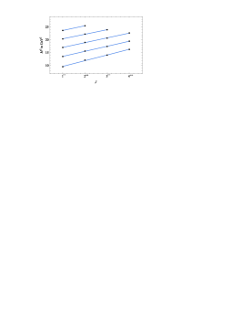
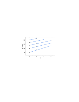
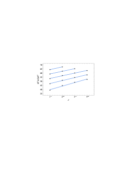
Figure 1: Parent and daughter Regge trajectories ($J,M^{2}$) for charmonia (left), bottomonia (middle) and $B_{c}$ (right) mesons with natural parity ($P=(-1)^{J}$).

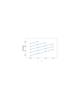
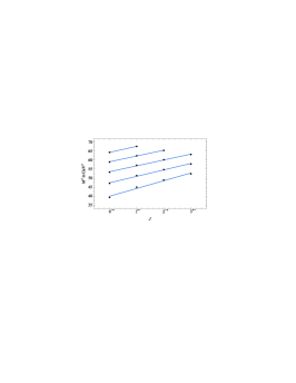
Figure 2: Parent and daughter Regge trajectories ($J,M^{2}$) for charmonia (left), bottomonia (middle) and $B_{c}$ (right) mesons with unnatural parity ($P=(-1)^{J+1}$).

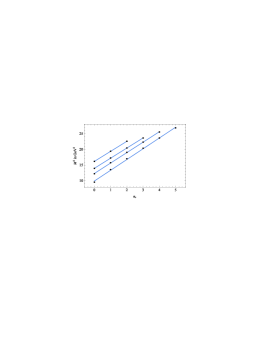
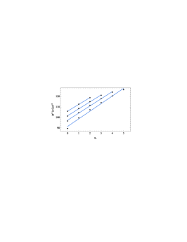
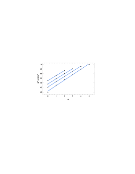
Figure 3: Parent and daughter Regge trajectories ($n_{r}\to M^{2}$) for charmonia (left), bottomonia (middle) and $B_{c}$ (right) mesons

According to the first principles of QCD, while the one-gluon-exchange interaction gives rise to employment of Coulomb potential with a strength proportional to the strong running coupling constant at very short distances, nonperturbative effect like confinement becomes prominent at larger distances. Charmonium belongs to neither purely nonrelativistic nor the relativistic regime where chiral symmetry breaking is more significant from physics point of view. Though Lattice QCD calculations in the quenched approximation have suggested a linearly increasing potential in the confinement range Dudek et al. (2008); Meinel (2009); Burch et al. (2010); Liu et al. (2012); McNeile et al. (2012); Daldrop et al. (2012); Kawanai and Sasaki (2014, 2011); Burnier et al. (2015); Kalinowski and Wagner (2015); Burnier et al. (2016), a specific form of interaction potential in the full range is not yet known. At short distances relativistic effects are more important as they give rise to quark-antiquark pairs from the vacuum that in turn affect the nonrelativistic Coulomb interaction in the presence of sea quarks. The mass spectra of quarkonia is not sensitive to these relativistic effects at short distances. However, the decay properties show significant difference with inclusion of relativistic corrections. We have used the most accepted available correction terms for computation of decay properties Lansberg and Pham (2009); Kwong et al. (1988); Barbieri et al. (1981); Mangano and Petrelli (1995) that improves the results significantly in most cases.

Using the potential parameters and numerical wave function, we compute the various decay properties of heavy quarkonia. We first compute the leptonic decay constants of pseudoscalar and vector mesons and our numerical results are tabulated in Tables 8 – 13. For the case of charmonia, our results are higher than those using LQCD and QCDSR Bečirević et al. (2014). In order to overcome this discrepancy, we include the QCD correction factors given in Ref. Braaten and Fleming (1995) and the results are tabulated in Table 8 and Table 9. After introducing the correction factors our results match with PDG, LQCD and QCDSR Bečirević et al. (2014) along with other theoretical models. We also compute the decay constants for excited $S$- wave charmonia and we found that our results are consistent with the other theoretical predictions. We also compute the decay constants of bottomonia and $B_{c}$ mesons. In this case, our results match with other theoretical predictions without incorporating the relativistic corrections. In the case of vector decay constants of bottomonia, our results are very close to experimental results as well as those obtained in LQCD Ref. Colquhoun et al. (2015). For the decay constants of $B_{c}$ mesons, we compare our results with nonrelativistic potential models Patel and Vinodkumar (2009); Monteiro et al. (2017).

Next we compute the digamma, digluon and dilepton decay widths using the relations Eqs. (13)–(16). Where the bracketed quantities are the first order radiative corrections to the decay widths. We compare our results with the available experimental results. We also compare our results with the theoretical models such as screened potential model Li and Chao (2009a, b), Martin-like potential model Shah et al. (2012), relativistic quark model (RQM) Ebert et al. (2003c, b), heavy quark spin symmetry Lansberg and Pham (2006), relativistic Salpeter model Kim et al. (2005) and other theoretical data.

Tables 14 and 15 we present our results for digamma decay widths for charmonia and bottomonia. Our results for $\Gamma(\eta_{c}\to\gamma\gamma)$ and $\Gamma(\eta_{c}(2S)\to\gamma\gamma)$ are higher than the experimental results. Experimental observation of the two photon decays of pseudoscalar states are considered as an important probe for identification of flavour as well as internal structure of mesons. The first order radiative correction (bracketed terms in Eq. (13)) was utilized to incorporate the difference and it is observed that our results along with the correction match with the experimental results Patrignani et al. (2016). We also compute the digamma decay width of excited charmonia. Our results for $P$-wave charmonia are higher than that of screened potential model Li and Chao (2009a) and relativistic quark model Ebert et al. (2003c). Our results for $\Gamma(\eta_{b}\to\gamma\gamma)$ match quite well with the experimental data while computed $\Gamma(\eta_{b}(2S)\to\gamma\gamma)$ value is overestimated when compared with the PDG data. For the excited state of $S$-wave bottomonia, our results fall in between those obtained in screened potential model Li and Chao (2009b) and relativistic quark model with linear confinement Godfrey and Moats (2015). The scenario is similar with $P$-wave bottomonia and charmonia.

Di-gluon decay has substantial contribution to hadronic decay of quarkonia below $c\bar{c}$ and $b\bar{b}$ threshold. In Tables 16 and 17 we represent our results for digluon decay width of charmonia and bottomonia respectively. Our results for $\Gamma(\eta_{c}\to gg)$ match perfectly with the PDG data Patrignani et al. (2016) but in the case of $\Gamma(\eta_{c}(2S)\to gg)$ our result is higher than the PDG data. We also compare the results obtained with that of the relativistic Salpeter method Kim et al. (2005) and an approximate potential model Patel et al. (2016). It is seen from Table 16 that the relativistic corrections provide better results in case of $P$-wave charmonia where as that for bottomonia are underestimated in present calculations when compared to relativistic QCD potential model Gupta et al. (1996) and power potential model Parmar et al. (2010). As the experimental data of digluon annihilation of bottomonia are not available, the validity of either of the approaches can be validated only after observations in forthcoming experiments.

We present the result of dilepton decay widths in the Table 18 and 19 and it is observed that our results matches with the PDG data Patrignani et al. (2016) upto $n$ = 3 for both charmonia and bottomonia. The contribution of the correction factor is more significant in the excited states with compared to that in the ground states of the quarkonia, indicating different dynamics in the intermediate quark-antiquark distance. Our results are also in good accordance with the other theoretical models.

We present our results of $E1$ transitions in Tables 20 - 22 in comparison with theoretical attempts such as relativistic potential model Radford and Repko (2007), quark model Ebert et al. (2003a), nonrelativistic screened potential model Deng et al. (2017b); Li and Chao (2009a, b). We also compare our results of charmonia transitions with available experimental results. Our result for $\Gamma(\psi(2S)\to\chi_{cJ}(1P)+\gamma)$ is in good agreement with the experimental result for $J=0$ but our results for $J=1,2$ are higher than the PDG data. Our results also agree well for the transition $\Gamma(\chi_{c2}(1P)\to J/\psi+\gamma)$. We also satisfy the experimental constraints for the transition $\Gamma(1^{3}D_{1}\to\chi_{cJ}+\gamma)$ for $J=0,1,2$. Our results share the same range with the results computed in other theoretical models. The $E1$ transitions of bottomonia agree fairly well except for the channel $\Gamma(\Upsilon(3S)\to\chi_{bJ}(3P))$, where our results are higher than the experimental results. The comparison of our results of $E1$ transitions in $B_{c}$ mesons with relativistic quark model Ebert et al. (2003a); Godfrey (2004) and power potential model Devlani et al. (2014) are found to be in good agreement. In Tables 23 - 25, we present our results of $M1$ transitions and also compared with relativistic potential model Radford and Repko (2007), quark model Ebert et al. (2003a); Godfrey and Moats (2015), nonrelativistic screened potential model Deng et al. (2017a, b), power potential Devlani et al. (2014) as well as with available experimental results. Our results of $\Gamma({\text{n}}\psi\to{\text{n}^{\prime}}\eta_{c}+\gamma)$ are in very good agreement with the PDG data as well with the other theoretical predictions. Computed $M1$ transitions in $B_{c}$ mesons are also within the results obtained from theoretical predictions. The computed $M1$ transition of bottomonia are found to be higher than the PDG data and also theoretical predictions.

V Conclusion

In this article, we have reported a comprehensive study of heavy quarkonia in the framework of nonrelativistic potential model considering linear confinement with least number of free model parameters such as confinement strength and quark mass. They are fine tuned to obtain the corresponding spin averaged ground state masses of charmonia and bottomonia determined from experimental data. The parameters are then used to predict the masses of excited states. In order to compute mass spectra of orbitally excited states, we incorporate contributions from the spin dependent part of confined one gluon exchange potential perturbatively.

Our results are found to be consistent with available PDG data, LQCD, relativistic quark model and other theoretical potential models. We also compute the digamma, digluon and dilepton decay widths of heavy quarkonia using nonrelativistic Van-Royen Weiskopf formula. The first order radiative corrections in calculation of these decays provide satisfactory results for the charmonia while no such correction is needed in case of bottomonia for being purely nonrelativistic system. We employ our parameters in computation of $B_{c}$ spectroscopy employing the quark masses and mean value of confinement strength of charmonia and bottomonia and our results are also consistent with the PDG data. We also compute the weak decays of $B_{c}$ mesons and the computed life time is also consistent with the PDG data. It is interesting to note here that despite having a $c$ quark, the nonrelativistic calculation of $B_{c}$ spectroscopy is in very good agreement with experimental and other theoretical models.

References

- Eichten et al. (2008) E. Eichten, S. Godfrey, H. Mahlke, and J. L. Rosner, Rev. Mod. Phys. 80, 1161 (2008), eprint hep-ph/0701208.
- Godfrey and Olsen (2008) S. Godfrey and S. L. Olsen, Ann. Rev. Nucl. Part. Sci. 58, 51 (2008), eprint 0801.3867.
- Barnes and Olsen (2009) T. Barnes and S. L. Olsen, Int. J. Mod. Phys. A 24S1, 305 (2009).
- Brambilla et al. (2011) N. Brambilla et al., Eur. Phys. J. C 71, 1534 (2011), eprint 1010.5827.
- Brambilla et al. (2014) N. Brambilla et al., Eur. Phys. J. C 74, 2981 (2014), eprint 1404.3723.
- Andronic et al. (2016) A. Andronic et al., Eur. Phys. J. C 76, 107 (2016).
- Patrignani et al. (2016) C. Patrignani et al. (Particle Data Group), Chin. Phys. C 40, 100001 (2016).
- Dudek et al. (2008) J. J. Dudek, R. G. Edwards, N. Mathur, and D. G. Richards, Phys. Rev. D 77, 034501 (2008), eprint 0707.4162.
- Meinel (2009) S. Meinel, Phys. Rev. D 79, 094501 (2009), eprint 0903.3224.
- Burch et al. (2010) T. Burch, C. DeTar, M. Di Pierro, A. X. El-Khadra, E. D. Freeland, S. Gottlieb, A. S. Kronfeld, L. Levkova, P. B. Mackenzie, and J. N. Simone, Phys. Rev. D 81, 034508 (2010), eprint 0912.2701.
- Liu et al. (2012) L. Liu, G. Moir, M. Peardon, S. M. Ryan, C. E. Thomas, P. Vilaseca, J. J. Dudek, R. G. Edwards, B. Joo, and D. G. Richards (Hadron Spectrum), JHEP 07, 126 (2012), eprint 1204.5425.
- McNeile et al. (2012) C. McNeile, C. T. H. Davies, E. Follana, K. Hornbostel, and G. P. Lepage, Phys. Rev. D 86, 074503 (2012), eprint 1207.0994.
- Daldrop et al. (2012) J. O. Daldrop, C. T. H. Davies, and R. J. Dowdall (HPQCD Collaboration), Phys. Rev. Lett. 108, 102003 (2012), eprint 1112.2590.
- Kawanai and Sasaki (2014) T. Kawanai and S. Sasaki, Phys. Rev. D 89, 054507 (2014), eprint 1311.1253.
- Kawanai and Sasaki (2011) T. Kawanai and S. Sasaki, Phys. Rev. Lett. 107, 091601 (2011), eprint 1102.3246.
- Burnier et al. (2015) Y. Burnier, O. Kaczmarek, and A. Rothkopf, JHEP 12, 101 (2015), eprint 1509.07366.
- Kalinowski and Wagner (2015) M. Kalinowski and M. Wagner, Phys. Rev. D 92, 094508 (2015), eprint 1509.02396.
- Burnier et al. (2016) Y. Burnier, O. Kaczmarek, and A. Rothkopf, JHEP 10, 032 (2016), eprint 1606.06211.
- Hilger et al. (2015) T. Hilger, C. Popovici, M. Gomez-Rocha, and A. Krassnigg, Phys. Rev. D 91, 034013 (2015), eprint 1409.3205.
- Voloshin (2008) M. B. Voloshin, Prog. Part. Nucl. Phys. 61, 455 (2008), eprint 0711.4556.
- Cho et al. (2015) S. Cho, K. Hattori, S. H. Lee, K. Morita, and S. Ozaki, Phys. Rev. D 91, 045025 (2015), eprint 1411.7675.
- Gershtein et al. (1995) S. S. Gershtein, V. V. Kiselev, A. K. Likhoded, and A. V. Tkabladze, Phys. Rev. D 51, 3613 (1995).
- Kiyo and Sumino (2014) Y. Kiyo and Y. Sumino, Phys. Lett. B 730, 76 (2014), eprint 1309.6571.
- Liu et al. (2017) T. Liu, A. A. Penin, and A. Rayyan, JHEP 02, 084 (2017), eprint 1609.07151.
- Dowdall et al. (2014) R. J. Dowdall, C. T. H. Davies, T. Hammant, and R. R. Horgan (HPQCD Collaboration), Phys. Rev. D 89, 031502 (2014), [Erratum: Phys. Rev.D92,039904(2015)], eprint 1309.5797.
- Neubert (1994) M. Neubert, Phys. Rept. 245, 259 (1994), eprint hep-ph/9306320.
- Ebert et al. (2011) D. Ebert, R. N. Faustov, and V. O. Galkin, Eur. Phys. J. C 71, 1825 (2011), eprint 1111.0454.
- Ebert et al. (2009) D. Ebert, R. N. Faustov, and V. O. Galkin, Phys. Rev. D 79, 114029 (2009), eprint 0903.5183.
- Ebert et al. (2006) D. Ebert, R. N. Faustov, and V. O. Galkin, Eur. Phys. J. C 47, 745 (2006), eprint hep-ph/0511029.
- Ebert et al. (2003a) D. Ebert, R. N. Faustov, and V. O. Galkin, Phys. Rev. D 67, 014027 (2003a), eprint hep-ph/0210381.
- Ebert et al. (2003b) D. Ebert, R. N. Faustov, and V. O. Galkin, Mod. Phys. Lett. A 18, 1597 (2003b), eprint hep-ph/0304227.
- Ebert et al. (2003c) D. Ebert, R. N. Faustov, and V. O. Galkin, Mod. Phys. Lett. A 18, 601 (2003c), eprint hep-ph/0302044.
- Ebert et al. (2000) D. Ebert, R. N. Faustov, and V. O. Galkin, Phys. Rev. D 62, 034014 (2000), eprint hep-ph/9911283.
- Gupta and Radford (1981) S. N. Gupta and S. F. Radford, Phys. Rev. D 24, 2309 (1981).
- Gupta et al. (1982) S. N. Gupta, S. F. Radford, and W. W. Repko, Phys. Rev. D 26, 3305 (1982).
- Gupta and Radford (1982) S. N. Gupta and S. F. Radford, Phys. Rev. D 25, 3430 (1982).
- Pantaleone et al. (1986) J. T. Pantaleone, S. H. H. Tye, and Y. J. Ng, Phys. Rev. D 33, 777 (1986).
- Maung et al. (1993) K. M. Maung, D. E. Kahana, and J. W. Norbury, Phys. Rev. D 47, 1182 (1993).
- Radford and Repko (2007) S. F. Radford and W. W. Repko, Phys. Rev. D 75, 074031 (2007), eprint hep-ph/0701117.
- Radford and Repko (2011) S. F. Radford and W. W. Repko, Nucl. Phys. A 865, 69 (2011), eprint 0912.2259.
- Gupta et al. (1986) S. N. Gupta, S. F. Radford, and W. W. Repko, Phys. Rev. D 34, 201 (1986).
- Vinodkumar et al. (1999) P. C. Vinodkumar, J. N. Pandya, V. M. Bannur, and S. B. Khadkikar, Eur. Phys. J. A 4, 83 (1999).
- Pandya and Vinodkumar (2001) J. N. Pandya and P. C. Vinodkumar, Pramana 57, 821 (2001).
- Rai et al. (2008a) A. K. Rai, J. N. Pandya, and P. C. Vinodkumar, Eur. Phys. J. A 38, 77 (2008a), eprint 0901.1546.
- Pandya et al. (2015) J. N. Pandya, N. R. Soni, N. Devlani, and A. K. Rai, Chin. Phys. C 39, 123101 (2015), eprint 1412.7249.
- Devlani et al. (2014) N. Devlani, V. Kher, and A. K. Rai, Eur. Phys. J. A 50, 154 (2014).
- Parmar et al. (2010) A. Parmar, B. Patel, and P. C. Vinodkumar, Nucl. Phys. A 848, 299 (2010), eprint 1001.0848.
- Rai et al. (2002) A. K. Rai, R. H. Parmar, and P. C. Vinodkumar, J. Phys. G 28, 2275 (2002).
- Kumar Rai et al. (2005) A. Kumar Rai, P. C. Vinodkumar, and J. N. Pandya, J. Phys. G 31, 1453 (2005).
- Rai and Vinodkumar (2006) A. K. Rai and P. C. Vinodkumar, Pramana 66, 953 (2006), eprint hep-ph/0606194.
- Rai et al. (2008b) A. K. Rai, B. Patel, and P. C. Vinodkumar, Phys. Rev. C 78, 055202 (2008b), eprint 0810.1832.
- Patel and Vinodkumar (2009) B. Patel and P. C. Vinodkumar, J. Phys. G 36, 035003 (2009), eprint 0808.2888.
- Fabre De La Ripelle (1988) M. Fabre De La Ripelle, Phys. Lett. B 205, 97 (1988).
- Eichten et al. (1975) E. Eichten, K. Gottfried, T. Kinoshita, J. B. Kogut, K. D. Lane, and T.-M. Yan, Phys. Rev. Lett. 34, 369 (1975), [Erratum: Phys. Rev. Lett.36,1276(1976)].
- Eichten et al. (1978) E. Eichten, K. Gottfried, T. Kinoshita, K. D. Lane, and T.-M. Yan, Phys. Rev. D 17, 3090 (1978), [Erratum: Phys. Rev.D21,313(1980)].
- Eichten et al. (1980) E. Eichten, K. Gottfried, T. Kinoshita, K. D. Lane, and T.-M. Yan, Phys. Rev. D 21, 203 (1980).
- Quigg and Rosner (1979) C. Quigg and J. L. Rosner, Phys. Rept. 56, 167 (1979).
- Eichten and Feinberg (1981) E. Eichten and F. Feinberg, Phys. Rev. D 23, 2724 (1981).
- Barnes et al. (2005) T. Barnes, S. Godfrey, and E. S. Swanson, Phys. Rev. D 72, 054026 (2005), eprint hep-ph/0505002.
- Sauli (2012) V. Sauli, Phys. Rev. D 86, 096004 (2012), eprint 1112.1865.
- Leitão et al. (2014) S. Leitão, A. Stadler, M. T. Peña, and E. P. Biernat, Phys. Rev. D 90, 096003 (2014), eprint 1408.1834.
- Godfrey and Isgur (1985) S. Godfrey and N. Isgur, Phys. Rev. D 32, 189 (1985).
- Godfrey (2004) S. Godfrey, Phys. Rev. D 70, 054017 (2004), eprint hep-ph/0406228.
- Godfrey and Moats (2015) S. Godfrey and K. Moats, Phys. Rev. D 92, 054034 (2015), eprint 1507.00024.
- Deng et al. (2017a) W.-J. Deng, H. Liu, L.-C. Gui, and X.-H. Zhong, Phys. Rev. D 95, 034026 (2017a), eprint 1608.00287.
- Deng et al. (2017b) W.-J. Deng, H. Liu, L.-C. Gui, and X.-H. Zhong, Phys. Rev. D 95, 074002 (2017b), eprint 1607.04696.
- Fischer et al. (2015) C. S. Fischer, S. Kubrak, and R. Williams, Eur. Phys. J. A 51, 10 (2015), eprint 1409.5076.
- Lakhina and Swanson (2006) O. Lakhina and E. S. Swanson, Phys. Rev. D 74, 014012 (2006), eprint hep-ph/0603164.
- Segovia et al. (2016) J. Segovia, P. G. Ortega, D. R. Entem, and F. Fernández, Phys. Rev. D93, 074027 (2016), eprint 1601.05093.
- Patel et al. (2016) S. Patel, P. C. Vinodkumar, and S. Bhatnagar, Chin. Phys. C 40, 053102 (2016), eprint 1504.01103.
- Bonati et al. (2015) C. Bonati, M. D’Elia, and A. Rucci, Phys. Rev. D 92, 054014 (2015), eprint 1506.07890.
- Gutsche et al. (2014) T. Gutsche, V. E. Lyubovitskij, I. Schmidt, and A. Vega, Phys. Rev. D 90, 096007 (2014), eprint 1410.3738.
- Shah et al. (2012) M. Shah, A. Parmar, and P. C. Vinodkumar, Phys. Rev. D 86, 034015 (2012), eprint 1203.6184.
- Negash and Bhatnagar (2016) H. Negash and S. Bhatnagar, Int. J. Mod. Phys. E 25, 1650059 (2016), eprint 1508.06131.
- Bhaghyesh et al. (2011) Bhaghyesh, K. B. Vijaya Kumar, and A. P. Monteiro, J. Phys. G38, 085001 (2011).
- Li and Chao (2009a) B.-Q. Li and K.-T. Chao, Phys. Rev. D 79, 094004 (2009a), eprint 0903.5506.
- Li and Chao (2009b) B.-Q. Li and K.-T. Chao, Commun. Theor. Phys. 52, 653 (2009b), eprint 0909.1369.
- Quigg and Rosner (1977) C. Quigg and J. L. Rosner, Phys. Lett. B 71, 153 (1977).
- Martin (1980) A. Martin, Phys. Lett. B 93, 338 (1980), ISSN 0370-2693.
- Buchmuller and Tye (1981) W. Buchmuller and S. H. H. Tye, Phys. Rev. D 24, 132 (1981).
- Kwong and Rosner (1991) W.-k. Kwong and J. L. Rosner, Phys. Rev. D 44, 212 (1991).
- Eichten and Quigg (1994) E. J. Eichten and C. Quigg, Phys. Rev. D 49, 5845 (1994), eprint hep-ph/9402210.
- Abe et al. (1998) F. Abe et al. (CDF Collaboration), Phys. Rev. Lett. 81, 2432 (1998), eprint hep-ex/9805034.
- Abazov et al. (2008) V. M. Abazov et al. (D0 Collaboration), Phys. Rev. Lett. 101, 012001 (2008), eprint 0802.4258.
- Aaij et al. (2012) R. Aaij et al. (LHCb Collaboration), Phys. Rev. Lett. 109, 232001 (2012), eprint 1209.5634.
- Aaij et al. (2014) R. Aaij et al. (LHCb Collaboration), Eur. Phys. J. C 74, 2839 (2014), eprint 1401.6932.
- Aad et al. (2014) G. Aad et al. (ATLAS Collaboration), Phys. Rev. Lett. 113, 212004 (2014), eprint 1407.1032.
- Gupta and Johnson (1996) S. N. Gupta and J. M. Johnson, Phys. Rev. D 53, 312 (1996), eprint hep-ph/9511267.
- Bali et al. (2000) G. S. Bali, B. Bolder, N. Eicker, T. Lippert, B. Orth, P. Ueberholz, K. Schilling, and T. Struckmann (TXL, T(X)L), Phys. Rev. D 62, 054503 (2000), eprint hep-lat/0003012.
- Bali (2001) G. S. Bali, Phys. Rept. 343, 1 (2001), eprint hep-ph/0001312.
- Alexandrou et al. (2003) C. Alexandrou, P. de Forcrand, and O. Jahn, Nucl. Phys. Proc. Suppl. 119, 667 (2003), eprint hep-lat/0209062.
- Isgur and Karl (1978) N. Isgur and G. Karl, Phys. Rev. D 18, 4187 (1978).
- Vijaya Kumar et al. (1997) K. B. Vijaya Kumar, A. K. Rath, and S. B. Khadkikar, Pramana 48, 997 (1997).
- Lucha and Schoberl (1999) W. Lucha and F. F. Schoberl, Int. J. Mod. Phys. C10, 607 (1999), eprint hep-ph/9811453.
- Monteiro et al. (2017) A. P. Monteiro, M. Bhat, and K. B. Vijaya Kumar, Phys. Rev. D 95, 054016 (2017), eprint 1608.05782.
- Van Royen and Weisskopf (1967) R. Van Royen and V. F. Weisskopf, Nuovo Cim. A 50, 617 (1967), [Erratum: Nuovo Cim.A51,583(1967)].
- Braaten and Fleming (1995) E. Braaten and S. Fleming, Phys. Rev. D 52, 181 (1995).
- Berezhnoy et al. (1996) A. V. Berezhnoy, V. V. Kiselev, and A. K. Likhoded, Z. Phys. A 356, 89 (1996).
- Krassnigg et al. (2016) A. Krassnigg, M. Gomez-Rocha, and T. Hilger, J. Phys. Conf. Ser. 742, 012032 (2016), eprint 1603.07232.
- Bečirević et al. (2014) D. Bečirević, G. Duplančić, B. Klajn, B. Melić, and F. Sanfilippo, Nucl. Phys. B 883, 306 (2014), eprint 1312.2858.
- Wang (2006) G.-L. Wang, Phys. Lett. B 633, 492 (2006), eprint math-ph/0512009.
- Colquhoun et al. (2015) B. Colquhoun, R. J. Dowdall, C. T. H. Davies, K. Hornbostel, and G. P. Lepage, Phys. Rev. D 91, 074514 (2015), eprint 1408.5768.
- Ecklund et al. (2008) K. M. Ecklund et al. (CLEO Collaboration), Phys. Rev. D 78, 091501 (2008), eprint 0803.2869.
- Lees et al. (2010) J. P. Lees et al. (BABAR Collaboration), Phys. Rev. D 81, 052010 (2010), eprint 1002.3000.
- Ablikim et al. (2012) M. Ablikim et al. (BESIII Collaboration), Phys. Rev. D 85, 112008 (2012), eprint 1205.4284.
- Dudek and Edwards (2006) J. J. Dudek and R. G. Edwards, Phys. Rev. Lett. 97, 172001 (2006), eprint hep-ph/0607140.
- Chen et al. (2016) T. Chen et al. (CLQCD Collaboration), Eur. Phys. J. C 76, 358 (2016), eprint 1602.00076.
- Bodwin et al. (1995) G. T. Bodwin, E. Braaten, and G. P. Lepage, Phys. Rev. D 51, 1125 (1995), [Erratum: Phys. Rev.D55,5853(1997)], eprint hep-ph/9407339.
- Khan and Hoodbhoy (1996) H. Khan and P. Hoodbhoy, Phys. Rev. D 53, 2534 (1996), eprint hep-ph/9501409.
- Schuler et al. (1998) G. A. Schuler, F. A. Berends, and R. van Gulik, Nucl. Phys. B 523, 423 (1998), eprint hep-ph/9710462.
- Bodwin et al. (2006) G. T. Bodwin, D. Kang, and J. Lee, Phys. Rev. D 74, 014014 (2006), eprint hep-ph/0603186.
- Bodwin et al. (2008) G. T. Bodwin, H. S. Chung, D. Kang, J. Lee, and C. Yu, Phys. Rev. D 77, 094017 (2008), eprint 0710.0994.
- Lansberg and Pham (2009) J. P. Lansberg and T. N. Pham, Phys. Rev. D 79, 094016 (2009), eprint 0903.1562.
- Lansberg and Pham (2006) J. P. Lansberg and T. N. Pham, Phys. Rev. D 74, 034001 (2006), eprint hep-ph/0603113.
- Sang et al. (2016) W.-L. Sang, F. Feng, Y. Jia, and S.-R. Liang, Phys. Rev. D 94, 111501 (2016), eprint 1511.06288.
- Landau (1948) L. D. Landau, Dokl. Akad. Nauk Ser. Fiz. 60, 207 (1948).
- Yang (1950) C.-N. Yang, Phys. Rev. 77, 242 (1950).
- Kwong et al. (1988) W. Kwong, P. B. Mackenzie, R. Rosenfeld, and J. L. Rosner, Phys. Rev. D 37, 3210 (1988).
- Barbieri et al. (1981) R. Barbieri, M. Caffo, R. Gatto, and E. Remiddi, Nucl. Phys. B 192, 61 (1981).
- Mangano and Petrelli (1995) M. L. Mangano and A. Petrelli, Phys. Lett. B 352, 445 (1995), eprint hep-ph/9503465.
- Kim et al. (2005) C. S. Kim, T. Lee, and G.-L. Wang, Phys. Lett. B 606, 323 (2005), eprint hep-ph/0411075.
- Gupta et al. (1996) S. N. Gupta, J. M. Johnson, and W. W. Repko, Phys. Rev. D 54, 2075 (1996), eprint hep-ph/9606349.
- Gonzalez et al. (2003) P. Gonzalez, A. Valcarce, H. Garcilazo, and J. Vijande, Phys. Rev. D 68, 034007 (2003), eprint hep-ph/0307310.
- Brambilla et al. (2006) N. Brambilla, Y. Jia, and A. Vairo, Phys. Rev. D 73, 054005 (2006), eprint hep-ph/0512369.
- Li et al. (2011) D.-M. Li, P.-F. Ji, and B. Ma, Eur. Phys. J. C 71, 1582 (2011), eprint 1011.1548.
- Abd El-Hady et al. (1999) A. Abd El-Hady, M. A. K. Lodhi, and J. P. Vary, Phys. Rev. D 59, 094001 (1999), eprint hep-ph/9807225.