Scaling relations in large-Prandtl-number natural thermal convection

Abstract

In this study we follow Grossmann and Lohse, Phys. Rev. Lett. 86, 3316 (2001), who derived various scalings regimes for the dependence of the Nusselt number Nu and the Reynolds number Re on the Rayleigh number Ra and the Prandtl number $\Pr$. We focus on theoretical arguments as well as on numerical simulations for the case of large-Pr natural thermal convection. Based on an analysis of self-similarity of the boundary layer equations, we derive that in this case the limiting large-Pr boundary-layer dominated regime is I${}_{\infty}^{<}$, introduced and defined in Grossmann and Lohse (2001), with the scaling relations $\text{Nu}\sim\text{Pr}^{0}\,\text{Ra}^{1/3}$ and $\text{Re}\sim\text{Pr}^{-1}\,\text{Ra}^{2/3}$. Our direct numerical simulations for Ra from $10^{4}$ to $10^{9}$ and $\Pr$ from 0.1 to 200 show that the regime I${}_{\infty}^{<}$ is almost indistinguishable from the regime III_∞, where the kinetic dissipation is bulk-dominated. With increasing Ra, the scaling relations undergo a transition to those in IV_u of reference Grossmann and Lohse (2001), where the thermal dissipation is determined by its bulk contribution.

I Introduction

Thermal convection flows are common in nature and technology. One of the classical systems to study such flows is Rayleigh–Bénard convection (RBC) Ahlers et al. (2009); Bodenschatz et al. (2000); Lohse and Xia (2010); Chillà and Schumacher (2012), where a fluid is confined between a heated bottom plate and a cooled top plate. In RBC the main input or control parameters of the system are the Rayleigh number $\text{Ra}\equiv\alpha g\Delta H^{3}/(\kappa\nu)$, the Prandtl number $\text{Pr}\equiv\nu/\kappa$, and the cell geometry. Here $\nu$ denotes the kinematic viscosity, $\kappa$ the thermal diffusivity, $\alpha$ the isobaric thermal expansion coefficient of the fluid, $g$ the acceleration due to gravity, $H$ the distance between the top and bottom plates, and $\Delta\equiv T_{+}-T_{-}>0$  with $T_{+}$ and $T_{-}$ the temperatures of, respectively, the heated bottom and the cooled top plates.

The main global response characteristics of this convective system are the mean convective heat transport from bottom to top and the mean momentum transport by convection, which are represented, respectively, by the Nusselt number Nu and the Reynolds number Re. How Nu and Re depend on Ra and Pr is the main issue in investigations of thermally driven flows.

The kinetic and the thermal dissipation rates are fundamental concepts in turbulent thermal convection. For some convective flow configurations, including RBC, it is possible to derive analytical relations for the time- and volume-averaged kinetic and thermal dissipation rates $\epsilon_{u}$ and $\epsilon_{\theta}$ in terms of Ra and Nu cf. Ahlers et al. (2009); Grossmann and Lohse (2000). For example, in RBC, it holds:

$$\epsilon_{u} = (\nu^{3}/H^{4})(\text{Nu}-1)\text{Ra}\,\text{Pr}^{-2},$$ (1)

$$\epsilon_{\theta} = (\kappa\Delta^{2}/H^{2})\,\text{Nu}.$$ (2)

Using these relations, Grossmann and Lohse developed a scaling theory (GL theory) Grossmann and Lohse (2000, 2001, 2002, 2003, 2004, 2011); Stevens et al. (2013), which is based on a decomposition of $\epsilon_{u}$ and $\epsilon_{\theta}$ into their boundary-layer (BL) and bulk contributions. Basically, the so-called scaling regimes I, II, III, and IV in the GL theory are associated with the BL–BL, bulk–BL, BL–bulk and bulk–bulk dominance in $\epsilon_{u}$ and $\epsilon_{\theta}$, respectively. The assigned subscripts $u$ and $\ell$ to these regimes indicate the $u$pper-Pr and $\ell$ower-Pr cases, respectively. Equating $\epsilon_{u}$ and $\epsilon_{\theta}$ to their estimated either bulk or BL contributions and employing the Prandtl–Blasius BL theory Prandtl (1905); Blasius (1908); Landau and Lifshitz (1987); Schlichting and Gersten (2000) for the thermal and viscous BL thicknesses, theoretically possible limiting scaling regimes followed. In particular, for the case of large $\Pr$-number thermal convection, the various possible scaling regimes I_u, I${}_{\infty}^{<}$, I${}_{\infty}^{>}$, II_u, III_u, III_∞, IV_u were obtained, see Grossmann and Lohse Grossmann and Lohse (2001) for the details.

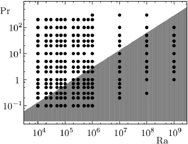
Figure 1: Sketch of the conducted DNS (symbols) in an (Ra, $\Pr$) plane. White region corresponds to the scaling regimes I${}_{\infty}^{<}$ and III_∞. Shadowed region corresponds to transition to other regimes.

In this paper we first derive a scaling relation between Re, Nu, and Pr in natural boundary-layer dominated thermal convection, in which the complete convective flow is due to temperature differences without any externally controlled wind input. This relation implies that in RBC the limiting large-Pr boundary-layer dominated regime is I${}_{\infty}^{<}$, with the scaling relations $\text{Nu}\sim\text{Pr}^{0}\,\text{Ra}^{1/3}$ and $\text{Re}\sim\text{Pr}^{-1}\,\text{Ra}^{2/3}$. This regime I${}_{\infty}^{<}$ matches the regime III_∞ for larger Ra, which in turn adjoins the regime IV_u for even higher Rayleigh numbers. Based on the results of our direct numerical simulations (DNS) of RBC in a cylindrical container of aspect ratio 1, for Ra ranging from $10^{4}$ to $10^{9}$ and $\Pr$ from 0.1 to 200, we demonstrate the correctness of the derived scaling relations in regime I${}_{\infty}^{<}$ and also the transition to regime IV_u for sufficiently large Ra.

II Relation between Re, Nu, and Pr in natural (purely thermally driven) boundary-layer dominated thermal convection

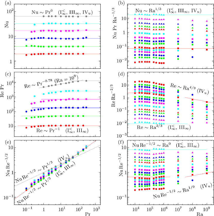
Figure 2: Nusselt number, Reynolds number and their combinations, as functions of the Prandtl number (a, c, e) and of the Rayleigh number (b, d, f), as obtained in the DNS of RBC in a cylindrical container of the aspect ratio 1, for (a, c, e) $\text{Ra}=10^{4}$ (red), $\text{Ra}=10^{5}$ (green), $\text{Ra}=10^{6}$ (blue), $\text{Ra}=10^{7}$ (magenta), $\text{Ra}=10^{8}$ (cyan) and $\text{Ra}=10^{9}$ (grey) and for (b, d, f) $\Pr=0.1$ (red circles), $\Pr=0.2$ (green circles), $\Pr=0.3$ (blue circles), $\Pr=0.5$ (magenta circles), $\Pr=0.7$ (cyan circles), $\Pr=1$ (red squares), $\Pr=2$ (green squares), $\Pr=3$ (blue squares), $\Pr=5$ (magenta squares), $\Pr=10$ (cyan squares), $\Pr=20$ (red triangles), $\Pr=30$ (green triangles), $\Pr=50$ (blue triangles), $\Pr=100$ (magenta triangles), $\Pr=200$ (cyan triangles).

Following Prandtl Prandtl (1905), we consider a fluid flow along a heated plate and choose the coordinate system such that the $x$ direction is along the plate and the $z$ direction is pointing vertically away from the plate. We assume that the mean flow in the other horizontal direction ($y$) is much weaker than that in $x$ or $z$ and, therefore, consider a two-dimensional flow that depends on $x$ and $z$ only. Under the standard Prandtl BL approximation Landau and Lifshitz (1987); Schlichting and Gersten (2000) we obtain the following momentum (3) and thermal (4) BL equations for a fluid motion near the isothermally heated horizontal plate:

$$u_{x}\partial_{x}u_{x}+u_{z}\partial_{z}u_{x} = \nu\partial^{2}_{z}u_{x}+\beta\alpha g(T-T_{0}),$$ (3)

$$u_{x}\partial_{x}T+u_{z}\partial_{z}T = \kappa\partial^{2}_{z}T,$$ (4)

where $T(x,z)$ denotes the temperature field above the plate, $(u_{x},u_{z})$ is the velocity vector in the coordinates $(x,z)$ and in the buoyancy term $\beta\alpha g(T-T_{0})$ we have $\beta$ vanishing in the case of a horizontal heated plate and $\beta=1$ in the case of vertical heated plate. The temperature boundary conditions are

$$T(x,0)=T_{+}, T(x,\infty)=T_{0}\equiv(T_{+}+T_{-})/2$$ (5)

and the velocity vanishes at the plate,

$$u_{x}(x,0)=u_{z}(x,0)=0,$$ (6)

due to the assumed no-slip boundary conditions. In the classical Prandtl–Blasius approach Prandtl (1905); Blasius (1908); Landau and Lifshitz (1987), a constant flow above an infinite horizontal plate is considered, which is parallel to the plate. This leads to the next boundary condition for the velocity, far away from the plate, $u_{x}(x,\infty)=U\neq 0$, where $U$ is the so-called wind outside the BL. The resulting Prandtl–Blasius approximation of the thermal boundary layer in laminar thermal convection is widely used, see, e.g. Grossmann and Lohse (2000); Zhou and Xia (2010). This approach can be generalized to include the influence of the turbulent fluctuations within the BL Shishkina et al. (2015); Ching et al. (2017); Ching (1997) and also can be adapted to the case of a non-vanishing pressure gradient within the BL (or to the case of a non-constant wind above the horizontal isothermal plate, which approaches the plate at arbitrary angle), see Shishkina et al. (2013, 2014). In all these cases the wind does not vanish in the bulk and, generally speaking, is artificially imposed in the boundary layer equations.

In natural thermal convection, where no mean flow is imposed in the core part of the domain, all the wind above the BL is self-organized. At the plate its absolute value is equal to zero. With growing distance from the plate, the absolute value of the wind first increases and, after it has achieved its maximum, slowly vanishes back to zero. The maximum value of the wind can be then considered as the reference quantity $U$. The magnitude of $U$ and the location, where the maximum of the wind is achieved, depends implicitly on Ra and Pr. Such approach was considered for the case of vertical convection (between two isothermal differently heated vertical walls) in Shishkina Shishkina (2016). Here we use the ideas from Shishkina (2016), to derive a relation between the Nusselt number Nu and the Reynolds number Re in laminar natural convection for the case, where gravity is orthogonal to the isothermally heated plate, i.e., to the RBC case.

The idea of the method suggested in Shishkina (2016) is the following. Let us construct a similarity variable $\xi$ as the usual combination of the vertical and horizontal coordinates, but now also with introduced Prandtl number and Rayleigh number:

$$\xi = \text{Pr}^{a}\text{Ra}^{b}(x/L)^{c}(z/H).$$ (7)

Here $L$ is the length of the heated plate and the exponents $a$, $b$ and $c$ are not fixed for the time being. In a similar way we introduce the exponents $d$, $e$, and $f$ for, respectively, Pr, Ra, and $x$ into the stream-function $\Psi$:

$$\Psi = \nu\text{Pr}^{d}\text{Ra}^{e}(x/L)^{f}\phi(\xi),$$ (8)

from which the velocity components in horizontal and vertical directions can be evaluated as $u_{x}=\partial_{z}\Psi$ and $u_{z}=-\partial_{x}\Psi$. The temperature $T$ is represented though a non-dimensional temperature $\theta$ as follows:

$$T = T_{0}+(T_{+}-T_{0})\theta(\xi)=T_{0}+(\Delta/2)\theta(\xi).$$ (9)

The Nusselt number can then be calculated as

$$\text{Nu}\equiv\frac{-L^{-1}\int_{0}^{L}\left.\kappa\partial_{z}T\right|_{z=0}\,dx}{\kappa\Delta/H}=\frac{-\theta^{\prime}(0)}{2(c+1)}\text{Pr}^{a}\text{Ra}^{b},$$ (10)

where $\theta^{\prime}\equiv d\theta/d\xi$ is the derivative of $\theta$ with respect to the similarity variable $\xi$. Analogously we can derive the Reynolds number, which is defined in terms of the maximal mean velocity along the heated plate:

$$\text{Re}\equiv UH/\nu,\quad U\equiv\max_{z}L^{-1}\int_{0}^{L}u_{x}\,dx.$$ (11)

Here the horizontal velocity $u_{x}$ equals

$$u_{x}=\partial_{z}\Psi=\text{Pr}^{a+d}\text{Ra}^{b+e}(\nu/H)(x/L)^{c+f}\phi^{\prime}.$$ (12)

Assuming that the maximal velocity is achieved at a certain value of $\xi=\hat{\xi}$, where $\phi^{\prime\prime}(\hat{\xi})=0$, from (11) and (12) we obtain

$$\text{Re}=\text{Pr}^{a+d}\text{Ra}^{b+e}{(c+f+1)}^{-1}{\phi^{\prime}(\hat{\xi})}.$$ (13)

This together with (10) yields

$$\frac{\text{Nu}}{\text{Re}^{1/2}\,\text{Pr}^{1/2}}=-\frac{\sqrt{c+f+1}}{2(c+1)}\frac{\theta^{\prime}(0)}{\;[\phi^{\prime}(\hat{\xi})]^{1/2}}\text{Pr}^{(a-d-1)/2}\text{Ra}^{(b-e)/2}.$$ (14)

Now we substitute (7)–(9) into the BL energy equation (4) and require the independence of the resulting BL equation from Pr and Ra. The equation then takes the following form:

$$\text{Pr}^{a}\text{Ra}^{b}(x/L)^{c}(1/H)\theta^{\prime\prime}\qquad\qquad\qquad\qquad\qquad$$

$$+f\text{Pr}^{d+1}\text{Ra}^{e}(x/L)^{f-1}(1/L)\phi\,\theta^{\prime}=0,$$ (15)

which implies

$$d=a-1,\quad e=b,\quad f=c+1.$$ (16)

The BL energy equation (II) then reduces to

$$\theta^{\prime\prime}+\frac{c+1}{\Gamma}\phi\,\theta^{\prime}=0$$ (17)

with the aspect ratio $\Gamma\equiv L/H$. Note that the boundary conditions for $\phi$ and $\theta$ are also independent of Pr and Ra, i.e., $\phi(0)=\phi^{\prime}(0)=0$, $\phi^{\prime}(\infty)=0$, and $\theta(0)=1$, $\theta(\infty)=0$, which one can obtain from (5)–(9).

With (16), the relation (14) is reduced to

$$\frac{\text{Nu}}{\text{Re}^{1/2}\,\text{Pr}^{1/2}}=-\frac{1}{\sqrt{2(c+1)}}\frac{\theta^{\prime}(0)}{\;[\phi^{\prime}(\hat{\xi})]^{1/2}}\text{Pr}^{0}\text{Ra}^{0}.$$ (18)

The momentum equation (3) with the similarity variable (7) and the stream-function (8) with the constants (16) takes the form

$$\text{Pr}^{4a}\phi_{\xi\xi\xi} + \text{Pr}^{4a-1}[(c+1)\phi\phi_{\xi\xi}-(2c+1)(\phi_{\xi})^{2}]$$ (19)

$$- \beta\,\text{Ra}^{1-4b}(x/H)^{-4c-1}\theta/2=0.$$

With a proper choice of the constant $b$ ($b=1/4$ for $\beta\neq 0$) this equation can be released from the Ra-dependence. However, as one can see from the comparison of the first two terms in (19), it cannot be made generally independent of Pr. However, for $\text{Pr}\gg 1$, the second term in (19) becomes negligible compared to the first term, which means that for $\text{Pr}\rightarrow\infty$ there exist certain values of $a$, $b$, $c$, $d$, $e$, and $f$ in (7) and (8) such that the governing momentum (3) and thermal (4) BL equations, written in terms of $\phi(\xi)$ and $\theta(\xi)$, as well as their boundary conditions, do not explicitly involve Pr and Ra. In this case, the solutions of the resulting BL equations, i.e., the functions $\phi(\xi)$ and $\theta(\xi)$, are also independent of Pr and Ra. In particular, the value of $\;{\theta^{\prime}(0)}{\,[\phi^{\prime}(\hat{\xi})]^{-1/2}}$ is a pure constant. This together with (18) immediately imply the following scaling relation for the Nusselt number with the Reynolds and the Prandtl numbers, which thus in general holds for natural boundary-layer dominated large-Prandtl-number thermal convection:

$$\text{Nu}\sim\text{Re}^{1/2}\,\text{Pr}^{1/2}.$$ (20)

Note that apart from RBC, the scaling (20) was found also in other different configurations of natural large-Prandtl-number thermal convective flows, for example, in horizontal convection, where the fluid layer is heated through one region of the bottom and cooled through another region of the bottom Shishkina and Wagner (2016); Shishkina et al. (2016); Hughes and Griffiths (2008) and also in vertical convection, where the fluid is heated through one vertical surface of the fluid layer and cooled though another vertical surface Shishkina (2016); Ng et al. (2015).

Previously Grossmann and Lohse (2000) it was shown that the relation (20) holds also for $\text{Pr}\ll 1$ in laminar Rayleigh–Bénard convection. Since the Pr-dependence as in (20) holds only for very large or small Pr, it formally breaks down for intermediate values of Pr, which strictly speaking means the absence of the similarity solution. However, also in this case relation (20) provides a fair estimate due to the fact that $\text{Pr}\approx 1$ in this regime and taking this value to some power does not introduce a strong Pr-dependence. Therefore, relation (20) effectively and in good approximation holds for all Prandtl numbers, which is fully supported by our simulations as we will see in the next section.

III Scalings of Re and Nu with Ra and Pr in boundary-layer dominated large-Pr RBC (regime I${}_{\infty}^{<}$)

In order to obtain the second scaling relation, in addition to (20), we follow Grossmann and Lohse (2000) for the BL-dominated thermal convection. The balance of the time- and volume-averaged kinetic dissipation rate $\epsilon_{u}$ to its estimated BL contribution gives ${\epsilon_{u}}\sim(\nu U^{2}/\lambda_{u}^{2})(\lambda_{u}/H)$, where $\lambda_{u}$ is the thickness of the viscous BL near the bottom plate. This together with Prandtl’s relation $\lambda_{u}/H\sim\text{Re}^{-1/2}$ for laminar RBC flows Landau and Lifshitz (1987); Schlichting and Gersten (2000) yields ${\epsilon_{u}}\sim(\nu^{3}/H^{4})\text{Re}^{5/2}$. Thus, from (1), (20) and the last relation one obtains the scalings in the laminar low-Pr regime I_ℓ of the GL theory:

Nu $$\sim \text{Pr}^{1/8}\text{Ra}^{1/4},$$ (21)

Re $$\sim \text{Pr}^{-3/4}\text{Ra}^{1/2}.$$ (22)

These scalings have been supported by numerous experimental and numerical RBC studies in the respective regions of the $(\text{Pr},\,\text{Ra})$ plane, see, e.g., Kerr (1996); Cioni et al. (1997); Verzicco and Camussi (1999, 2003); van der Poel et al. (2012); Stevens et al. (2013); Petschel et al. (2013); therefore in the present work we do not focus on the low-Pr regime I_ℓ.

With decreasing Ra, the viscous BL thickness $\lambda_{u}$ generally increases and slowly saturates to a certain bounding value, which is comparable with $H$ Grossmann and Lohse (2001). In this case the BL contribution to the mean kinetic dissipation rate scales as ${\epsilon_{u}}\sim(\nu U^{2}/H^{2})$, which yields

$${\epsilon_{u}}\sim(\nu^{3}/H^{4})\text{Re}^{2}.$$ (23)

Thus, from (1), (20) and (23) the scaling relations in the regime I${}_{\infty}^{<}$ of BL-dominated large-Pr RBC follow,

Nu $$\sim \text{Pr}^{0}\,\text{Ra}^{1/3},$$ (24)

Re $$\sim \text{Pr}^{-1}\,\text{Ra}^{2/3}.$$ (25)

Note that these obtained scaling relations (24), (25) are similar to those in the regime III_∞ Grossmann and Lohse (2001), although in the regime III_∞ the kinetic dissipation turns to be bulk-dominated.

The relations (24), (25) hold up to very large Pr. The DNS for $\text{Pr}=2548$ and Ra up to $10^{9}$ Horn et al. (2013) showed that $\text{Nu}\sim\text{Ra}^{0.3}$ and $\text{Re}\sim\text{Ra}^{0.6}$. Independence of the Nusselt number of the Prandtl number for large Pr was demonstrated also in several other DNS, see, e.g. van der Poel et al. (2013); Petschel et al. (2013). The measurements by Xia et al. (2002) for Pr from 4 to 1350 and Ra up to $3\times 10^{10}$ also demonstrated that Nu roughly goes as $\text{Ra}^{0.3}$ and is almost independent of Pr.

The results of our present DNS, which were conducted using the finite-volume code goldfish (see, e.g., Shishkina et al. (2015); Shishkina and Horn (2016)) for RBC for Ra from $10^{4}$ to $10^{9}$ and $\Pr$ from 0.1 to 200, are summarized in Fig. 2. In the left column (Fig. 2 a, c, e) the Prandtl number dependences and in the right column (Fig. 2 b, d, f) the Rayleigh number dependences are presented for the Nusselt number (Fig. 2 a, b), Reynolds number (Fig. 2 c, d) and their combination $\text{Nu}\,\text{Re}^{-1/2}$, due to the relation (20).

One can see that through several decades of Pr and Ra, the Nusselt number remains to be independent of Pr (Fig. 2a) and scales with the Rayleigh number as $\sim\text{Ra}^{1/3}$ (Fig. 2b), in full agreement with (24). Note that also for the larger Ra this scaling should hold, as on this end the regime III_∞ enters the regime IV_u Grossmann and Lohse (2000, 2001) with its scaling relations:

Nu $$\sim \text{Pr}^{0}\,\text{Ra}^{1/3},$$ (26)

Re $$\sim \text{Pr}^{-2/3}\,\text{Ra}^{4/9}.$$ (27)

For the smallest Pr ($\text{Pr}<0.5$ in Fig. 2a), the Nusselt number slightly grows with Pr, as the flow undergoes a transition from the regime I${}_{\infty}^{<}$ to the regime I_ℓ, with its own scaling (21).

From Fig. 2c we can conclude the following: For sufficiently large Pr ($\text{Pr}\geq 0.5$) and moderate Ra ($\text{Ra}<10^{9}$), the Reynolds number scales as $\text{Re}\sim\text{Pr}^{-1}$ through several decades of Pr, as it should be in the regimes I${}_{\infty}^{<}$ and III_∞, see (25). Again, the region of very small Pr, $\text{Pr}<0.5$, belongs to the scaling regime I_ℓ (22) and, therefore, the values of (Re Pr) increase with increasing Pr. The large-Ra region is already around the transition to the regime IV_u, where the scaling (27) should take over. For $\text{Ra}=10^{9}$, the Reynolds number behaves already as $\text{Re}\sim\text{Pr}^{-0.78}$, as our simulations show. Fig. 2d also supports the scaling (25), but this time with respect to the Ra-scaling in large-Pr BL-dominated RBC. Indeed, Re goes as $\sim\text{Ra}^{2/3}$ there, with a tendency to $\sim\text{Ra}^{4/9}$ (27), as it should be in the scaling regime IV_u (this slope is shown in Fig. 2d with a red inclined line).

Finally, in Fig. 2f one can see that $\text{Nu}\,\text{Re}^{-1/2}$ in the regimes I${}_{\infty}^{<}$ and III_∞ is independent of Ra. For larger Ra, this quantity starts to increase and tends to $\text{Nu}\,\text{Re}^{-1/2}\sim\text{Ra}^{1/9}$, as it should be in the scaling regime IV_u (this slope is shown in Fig. 2f with a red inclined line). The Prandtl-number dependences of $\text{Nu}\,\text{Re}^{-1/2}$ in Fig. 2e also support the scaling relations (24), (25) for the regimes I${}_{\infty}^{<}$ and III_∞ and the scaling relations (26), (27) for the regime IV_u, i.e. it varies from $\text{Nu}\,\text{Re}^{-1/2}\sim\text{Pr}^{1/2}$ for smaller Ra to $\text{Nu}\,\text{Re}^{-1/2}\sim\text{Pr}^{1/3}$ for larger Ra.

IV Conclusions

In the present work we derived that the relation $\text{Nu}\sim\text{Re}^{1/2}\Pr^{1/2}$ holds in laminar natural thermal convection, where no wind is imposed above the isothermal plate, for large Prandtl numbers $\text{Pr}\gg 1$. Our derivation is based on a generalization of the Prandtl approach Prandtl (1905) and on a search of a similarity solution of the laminar thermal BL equation when $\text{Pr}\rightarrow\infty$. The scaling relation (20), $\text{Nu}\sim\text{Re}^{1/2}\Pr^{1/2}$, which holds for all Prandtl numbers in laminar Rayleigh–Bénard convection, holds more generally also in the non-laminar regimes. It strictly holds for very large or very small Pr, but formally breaks down for intermediate Pr. However, as in this case $\text{Pr}\sim 1$, the relation $\text{Nu}\sim\text{Re}^{1/2}\Pr^{1/2}$ still provides a good approximation of the relationship between Re, Pr and Nu also in this regime, which is fully supported by our simulations in a wide parameter range.

Because of the relation (20), the limiting large-$\Pr$ laminar regime in RBC is regime I${}_{\infty}^{<}$ with the scaling relations (24), (25), which were originally derived in Grossmann and Lohse (2001) as one of the possible scaling regimes in large-Pr thermal convection.

Based on our DNS data for Ra from $10^{4}$ to $10^{9}$ and Pr from 0.1 to 200 (totally $200$ cases), we showed that the scaling regime I${}_{\infty}^{<}$ undergoes a smooth transition into regime III_∞, so that one does not necessarily have to distinguish them. For sufficiently large Ra, the scaling relations in regime III_∞ undergo a transition to those of regime IV_u. All these scaling relations and transitions have been supported by our DNS over a large range of Ra and Pr.