Bilinear Assignment Problem: Large Neighborhoods and Experimental Analysis of Algorithms

Abstract

The bilinear assignment problem (BAP) is a generalization of the well-known quadratic assignment problem (QAP). In this paper, we study the problem from the computational analysis point of view. Several classes of neigborhood structures are introduced for the problem along with some theoretical analysis. These neighborhoods are then explored within a local search and a variable neighborhood search frameworks with multistart to generate robust heuristic algorithms. Results of systematic experimental analysis have been presented which divulge the effectiveness of our algorithms. In addition, we present several very fast construction heuristics. Our experimental results disclosed some interesting properties of the BAP model, different from those of comparable models. This is the first thorough experimental analysis of algorithms on BAP. We have also introduced benchmark test instances that can be used for future experiments on exact and heuristic algorithms for the problem.

Keywords: bilinear assignment problem, quadratic assignment problem, average solution value, exponential neighborhoods, heuristics, local search, variable neighborhood search, VLSN search.

1 Introduction

Given a four dimensional array $Q=(q_{ijkl})$ of size $m\times m\times n\times n$, an $m\times m$ matrix $C=(c_{ij})$ and an $n\times n$ matrix $D=(d_{kl})$, the bilinear assignment problem (BAP) can be stated as:

Minimize $$\sum_{i=1}^{m}\sum_{j=1}^{m}\sum_{k=1}^{n}\sum_{l=1}^{n}q_{ijkl}x_{ij}y_{kl}+\sum_{i=1}^{m}\sum_{j=1}^{m}c_{ij}x_{ij}+\sum_{k=1}^{n}\sum_{l=1}^{n}d_{kl}y_{kl}$$ (1)

subject to $$\sum_{j=1}^{m}x_{ij}=1\qquad\qquad i=1,2,\ldots,m,$$ (2)

$$\sum_{i=1}^{m}x_{ij}=1\qquad\qquad j=1,2,\ldots,m,$$ (3)

$$\sum_{l=1}^{n}y_{kl}=1\qquad\qquad k=1,2,\ldots,n,$$ (4)

$$\sum_{k=1}^{n}y_{kl}=1\qquad\qquad l=1,2,\ldots,n,$$ (5)

$$x_{ij},\ y_{kl}\in\{0,1\}\qquad i,j=1,\ldots,m,\ \ k,l=1,\ldots,n.$$ (6)

If we impose additional restrictions that $m=n$ and $x_{ij}=y_{ij}$ for all $i,j$, BAP becomes equivalent to the well-known quadratic assignment problem (QAP) [5, 7]. As noted in [9], the constraints $x_{ij}=y_{ij}$ can be enforced without explicitly stating them by modifying the entries of $Q,$ $C$ and $D$. For example, replacing $c_{ij}$ by $c_{ij}+L$, $d_{ij}$ by $d_{ij}+L$ and $q_{ijij}$ by $q_{ijij}-2L$, for some large $L$ results in an increase in the objective function value by $\sum_{i,j=1}^{n}L(x_{ij}-2x_{ij}y_{ij}+y_{ij})=\sum_{i,j=1}^{n}L(x_{ij}-y_{ij})^{2}$. Since $L$ is large, in an optimal solution, $x_{ij}=y_{ij}$ is forced and hence the modified BAP becomes QAP. Therefore, BAP is also strongly NP-hard. Moreover, since the reduction described above preserves the objective values of the solutions that satisfy $x_{ij}=y_{ij}$, BAP inherits the approximability hardness of QAP [27]. That is, for any $\alpha>1$, BAP does not have a polynomial time $\alpha$-approximation algorithm, unless P=NP. Further, BAP is NP-hard even if $m=n$ and $Q$ is a diagonal matrix [9]. A special case of BAP, called the independent quadratic assignment problem, was studied by Burkard et al. [6] and identified polynomially solvable special cases.

Since BAP is a generalization of the QAP, all of the applications of QAP can be solved as BAP. In addition, BAP can be used to model other discrete optimization problems with practical applications. Tsui and Chang [29, 30] used BAP to model a door dock assignment problem. Consider a sorting facility of a large shipping company where $m$ loaded inbound trucks are arriving from different locations, and they need to be assigned to $m$ inbound doors of the facility. The shipments from the inbound trucks need to be transferred to $n$ outbound trucks, which carries the shipments to different customer locations. The sorting facility also has $n$ outbound doors for the outbound trucks. Let $w_{ij}$ denote the amount of items from $i$-th inbound truck that need to be transferred to $j$-th outbound truck/customer location, and let $d_{ij}$ denote the distance between the $i$-th inbound door and the $j$-th outbound door. Then the problem of assigning inbound trucks to inbound doors and outbound trucks to outbound doors, so that the total work needed to transfer all items from inbound to outbound trucks, is exactly BAP with costs $q_{ijkl}=w_{ik}d_{jl}$. Torki et al. [28] used BAP to develop heuristic algorithms for QAP with a low rank cost matrix. BAP also encompasses well-known disjoint matching problem [9, 11, 12] and axial 3-dimensional assignment problem [9, 24].

Despite the applicability and unifying capabilities of the model, BAP is not studied systematically from an experimental analysis point of view. In [29, 30], the authors proposed local search and branch and bound algorithms to solve BAP, but detailed computational analysis was not provided. The model was specially structured to focus on a single application, which limited the applicability of these algorithms for the general case. Torki et al. [28] presented experimental results on algorithms for low rank BAP in connection with developing heuristics for QAP. To the best of our knowledge, no other experimental studies on the model are available.

In this paper, we present various neighborhoods associated with a feasible solution of BAP and analyze their theoretical properties in the context of local search algorithms, particularly on the worst case behavior. Some of these neighborhoods are of exponential size but can be searched for an improving solution in polynomial time. Local search algorithms with such very large scale neighborhoods (VLSN) proved to be an effective solution approach for many hard combinatorial optimization problems [2, 3]. We also present extensive experimental results by embedding these neighborhoods within a variable neighborhood search (VNS) framework in addition to the standard and multi-start VLSN local search. Some very fast construction heuristics are also provided along with experimental analysis. Although local search and variable neighborhood search are well known algorithmic paradigms that are thoroughly investigated in the context of various combinatorial optimization problems, to achieve effectiveness and obtain superior outcomes variable neighborhood search algorithms needs to exploit special problem structures that efficiently link the various neighborhoods under consideration. In this sense, developing variable neighborhood search algorithms is always intriguing, especially when it comes to new optimization problems having several well designed neighborhood structures with interesting properties. Our experimental analysis shows that the average behavior of the algorithms are much better and the established negative worst case performance hardly occurs. Such a conclusion can only be made by systematic experimentation, as we have done. On a balance of computational time and solution quality, a multi-start based VLSN local search became our proposed approach. Although, by allowing significantly more time, a strategic variable neighborhood search outperformed this algorithm in terms of solution quality.

The rest of the paper is organized as follows. In Section 2 we specify notations and several relevant results that are used in the paper. In Section 3 we describe several construction heuristics for BAP that generate reasonable solutions, often quickly. In Section 4, we present various neighborhood structures and analyze their theoretical properties. We then (Section 5) describe in details specifics of our experimental setup as well as sets of instances that we have generated for the problem. The benchmark instances that we have developed are available upon request from Abraham Punnen (apunnen@sfu.ca) for other researchers to further study the problem. The development of these test instances and best-known solutions is yet another contribution of this work. Sections 6 and 7 deal with experimental analysis of construction heuristics and local search algorithms. Our computational results disclose some interesting and unexpected outcomes, particularly when comparing standard local search with its multi-start counterpart. In Section 8 we combine better performing construction heuristics and different local search algorithms to develop several variable neighborhood search algorithms and present comparison with our best performing multistart local search algorithm. Concluding remarks are presented in Section 9.

2 Notations and basic results

Let $\mathcal{X}$ be the set of all 0-1 $m\times m$ matrices satisfying (2) and (3) and $\mathcal{Y}$ be the set of all 0-1 $n\times n$ matrices satisfying (4) and (5). Also, let $\mathcal{F}$ be the set of all feasible solutions of BAP. Note that $|\mathcal{F}|=m!n!$. An instance of the BAP is completely represented by the triplet $(Q,C,D)$. Let $M=M^{\prime}=\{1,2,\ldots,m\}$ and $N=N^{\prime}=\{1,2,\ldots,n\}$. An $\mathbf{x}\in\mathcal{X}$ assigns each $i\in M$ a unique $j\in M^{\prime}$. Likewise, a $\mathbf{y}\in\mathcal{Y}$ assigns each $k\in N$ a unique $l\in N^{\prime}$. Without loss of generality we assume that $m\leq n$. For $\mathbf{x}\in\mathcal{X}$ and $\mathbf{y}\in\mathcal{Y}$, $f(\mathbf{x},\mathbf{y})$ denotes the objective function value of ($\mathbf{x},\mathbf{y}$).

Given an instance $(Q,C,D)$ of a BAP, let $\mathcal{A}(Q,C,D)$ be the average of the objective function values of all feasible solutions.

Theorem 1 (Ćustić et al. [9]).

${\displaystyle\mathcal{A}(Q,C,D)=\frac{1}{mn}\sum_{i=1}^{m}\sum_{j=1}^{m}\sum_{k=1}^{n}\sum_{l=1}^{n}q_{ijkl}+\frac{1}{m}\sum_{i=1}^{m}\sum_{j=1}^{m}c_{ij}+\frac{1}{n}\sum_{k=1}^{n}\sum_{l=1}^{n}d_{kl}}$.

Consider an equivalence relation $\sim$ on $\mathcal{F}$, where $(\mathbf{x},\mathbf{y})\sim(\mathbf{x}^{\prime},\mathbf{y}^{\prime})$ if and only if there exist $a\in\{0,1,\ldots,m-1\}$ and $b\in\{0,1,\ldots,n-1\}$ such that $x_{ij}=x^{\prime}_{i(j+a\mod m)}$ for all $i,j$, and $y_{kl}=y^{\prime}_{k(l+b\mod n)}$ for all $k,l$. Here and later in the paper we use the notation of $x_{i(j+a\mod m)}$ in a sense that, if $(j+a)\mod m=0$, we then assume it to refer to the variable $x_{im}$. Similar assumptions will be made for the other index of $x_{ij}$ and variables $y_{kl}$ to improve the clarity of presentation.

Let us consider an example of equivalence class for $\sim$. Given $a\in M$, $b\in N$ let $(\mathbf{x}^{a},\mathbf{y}^{b})\in\mathcal{F}$ be defined as

$$x_{ij}^{a}=\begin{cases}1&\text{if }j=i+a\mod m,\\ 0&\text{otherwise}\end{cases}\quad\text{and}\quad y_{kl}^{b}=\begin{cases}1&\text{if }l=k+b\mod n,\\ 0&\text{otherwise}.\end{cases}$$

Theorem 2 (Ćustić et al. [9]).

For any instance $(Q,C,D)$ of BAP

$$\min_{a\in M,b\in N}\{f(\mathbf{x}^{a},\mathbf{y}^{b})\}\leq\mathcal{A}(Q,C,D)\leq\max_{a\in M,b\in N}\{f(\mathbf{x}^{a},\mathbf{y}^{b})\}.$$

It can be shown that any equivalence class defined by $\sim$ can be used to obtain the type of inequalities stated above. Theorem 2 provides a way to find a feasible solution to BAP with objective function value no worse than $\mathcal{A}(Q,C,D)$ in $O(m^{2}n^{2})$ time. To achieve this, we search through the set of solutions defined by the equivalence class, with any feasible solution to BAP as a starting point.

A feasible solution $(\mathbf{x},\mathbf{y})$ to BAP is said to be no better than the average if $f(\mathbf{x},\mathbf{y})\geq A(Q,C,D)$. In [9] we have provided the following lower bound for the number of feasible solutions that are no better than the average.

Theorem 3 (Ćustić et al. [9]).

$|\{(\mathbf{x},\mathbf{y})\in\mathcal{F}\ \colon f(\mathbf{x},\mathbf{y})\geq A(Q,C,D)\}|\geq(m-1)!(n-1)!$.

An algorithm that is guaranteed to return a solution with the objective function value at most $\mathcal{A}(Q,C,D)$ guarantees a solution that is no worse than $(m-1)!(n-1)!$ solutions. Thus, the domination ratio [14, 8] of such an algorithm is $\frac{1}{mn}$.

3 Construction heuristics

In this section, we consider heuristic algorithms that will generate solutions to BAP using various construction approaches. Such algorithms are useful in situations where solutions of reasonable quality are needed quickly. These algorithms can also be used to generate starting solutions for more complex improvement based algorithms.

Our first algorithm, called Random, is the trivial approach of generating a feasible solution ($\mathbf{x},\mathbf{y}$). Both $\mathbf{x}$ and $\mathbf{y}$ are selected as random assignments in uniform fashion. It should be noted that the expected value of the solution produced by Random is precisely $\mathcal{A}(Q,C,D)$.

Let us now discuss a different randomized technique, called RandomXYGreedy. This algorithm builds a solution by randomly picking a ‘not yet assigned’ $i\in M$ or $k\in N$, and then setting $x_{ij}$ or $y_{kl}$ to $1$ for a ‘not yet assigned’ $j\in M^{\prime}$ or $l\in N^{\prime}$ so that the total cost of the resulting partial solution is minimized. A pseudo-code of RandomXYGreedy is presented in Algorithm 1. Here and later in the paper we will present description of the algorithms by assuming that the input BAP instance $(Q,C,D)$ has $C$ and $D$ as zero arrays. This restriction is for simplicity of presentation and does not affect neither the theoretical complexity of BAP nor the asymptotic computational complexity of the presented algorithms. It is easy to extend the algorithms to the general case in a straightforward way. The running time of RandomXYGreedy is $O(mn^{2})$ as each addition to our solution is selected using quadratic number of computations. However, just reading the data for the $Q$ matrix takes $O(m^{2}n^{2})$ time. For the rest of the paper we will consider running time of our algorithms without including this input overhead.

Algorithm 1 RandomXYGreedy

integers $m,n$; $m\times m\times n\times n$ array $Q$

feasible solution to BAP

$x_{ij}\leftarrow 0\,\forall i,j$; $y_{kl}\leftarrow 0\,\forall k,l$

while not all $i\in M$ and $k\in N$ are assigned do

    randomly pick some $i\in M$ or $k\in N$ that is unassigned

    if $i$ is picked then

       $j^{\prime}\leftarrow$ random $j\in M$ that is unassigned; $\Delta^{\prime}\leftarrow\sum_{k,l\in N}q_{ij^{\prime}kl}y_{kl}$

       for all $j\in M$ that is unassigned do

          $\Delta\leftarrow\sum_{k,l\in N}q_{ijkl}y_{kl}$ $\triangleright$ value change if $i$ assigned to $j$

          if $\Delta<\Delta^{\prime}$ then

             $j^{\prime}\leftarrow j$; $\Delta^{\prime}\leftarrow\Delta$

          end if

       end for

       $x_{ij^{\prime}}\leftarrow 1$ $\triangleright$ assign $i$ to $j^{\prime}$

    else

       $l^{\prime}\leftarrow$ random $l\in N$ that is unassigned; $\Delta^{\prime}\leftarrow\sum_{i,j\in M}q_{ijkl^{\prime}}x_{ij}$

       for all $l\in N$ that is unassigned do

          $\Delta\leftarrow\sum_{i,j\in M}q_{ijkl}x_{ij}$ $\triangleright$ value change if $k$ assigned to $l$

          if $\Delta<\Delta^{\prime}$ then

             $l^{\prime}\leftarrow l$; $\Delta^{\prime}\leftarrow\Delta$

          end if

       end for

       $y_{kl^{\prime}}\leftarrow 1$ $\triangleright$ assign $k$ to $l^{\prime}$

    end if

end while

return ($\mathbf{x}$, $\mathbf{y}$)

Our next algorithm is fully deterministic and is called Greedy (see Algorithm 2). This is similar to RandomXYGreedy, except that, at each iteration, we select the best available $x_{ij}$ or $y_{kl}$ to be added to the current partial solution. We start the algorithm by choosing the partial solution $x_{i^{\prime}j^{\prime}}=1$ and $y_{k^{\prime}l^{\prime}}=1$ where $i^{\prime},j^{\prime},k^{\prime},l^{\prime}$ correspond to a smallest element in the array $Q$. The total running time of this heuristic is $O(n^{3})$, considering that the position of the smallest $q_{i^{\prime}j^{\prime}k^{\prime}l^{\prime}}$ is provided.

Algorithm 2 Greedy

integers $m,n$; $m\times m\times n\times n$ array $Q$

feasible solution to BAP

$x_{ij}\leftarrow 0\,\forall i,j$; $y_{kl}\leftarrow 0\,\forall k,l$

$i^{\prime},j^{\prime},k^{\prime},l^{\prime}\leftarrow arg\,min_{i,j\in M,k,l\in N}q_{ijkl}$; $x_{i^{\prime}j^{\prime}}\leftarrow 1$; $y_{k^{\prime}l^{\prime}}\leftarrow 1$

while not all $i\in M$ and $k\in N$ are assigned do

    $\Delta^{\prime}_{x}\leftarrow\infty$; $\Delta^{\prime}_{y}\leftarrow\infty$

    for all $i\in M$ that is unassigned do

       for all $j\in M$ that is unassigned do

          $\Delta\leftarrow\sum_{k,l\in N}q_{ijkl}y_{kl}$ $\triangleright$ value change if $i$ assigned to $j$

          if $\Delta<\Delta^{\prime}_{x}$ then

             $i^{\prime}\leftarrow i$; $j^{\prime}\leftarrow j$; $\Delta^{\prime}_{x}\leftarrow\Delta$

          end if

       end for

    end for

    for all $k\in N$ that is unassigned do

       for all $l\in N$ that is unassigned do

          $\Delta\leftarrow\sum_{i,j\in M}q_{ijkl}x_{ij}$ $\triangleright$ value change if $k$ assigned to $l$

          if $\Delta<\Delta^{\prime}_{y}$ then

             $k^{\prime}\leftarrow k$; $l^{\prime}\leftarrow l$; $\Delta^{\prime}_{y}\leftarrow\Delta$

          end if

       end for

    end for

    if $\Delta^{\prime}_{x}\leq\Delta^{\prime}_{y}$ then

       $x_{i^{\prime}j^{\prime}}\leftarrow 1$ $\triangleright$ assign $i^{\prime}$ to $j^{\prime}$

    else

       $y_{k^{\prime}l^{\prime}}\leftarrow 1$ $\triangleright$ assign $k^{\prime}$ to $l^{\prime}$

    end if

end while

return ($\mathbf{x}$, $\mathbf{y}$)

Theorem 4.

The objective function value of a solution produced by the Greedy algorithm could be arbitrarily bad and could be worse than $\mathcal{A}(Q,C,D)$.

Proof.

Consider the following BAP instance: $C$ and $D$ are zero matrices and elements of $2\times 2\times 3\times 3$ matrix $Q$ are all zero except $q_{1111}=-\epsilon,q_{1122}=q_{1133}=\epsilon,q_{2211}=q_{1123}=q_{1132}=2\epsilon,q_{2222}=q_{2233}=L$, where $\epsilon$ and $L$ are arbitrarily small and large positive numbers, respectively. At first the algorithm will assign $x_{11}=y_{11}=1$, as $q_{1111}$ is the smallest element in the array. Next, all indices $i,j\in M$ such that $i,j>2$ and $k,l\in M$ such that $k,l>3$ will be assigned within their respective groups. This is due to the fact that any assignment in those sets adds no additional cost to the current partial solution. Following that, $y_{22}=y_{33}=1$ will be added. And finally, $x_{22}$ will be set to $1$ to complete a solution with the cost $3\epsilon+2L$. However, an optimal solution in this case will contain $x_{11}=x_{22}=y_{11}=y_{23}=y_{32}=1$ with an objective value of $5\epsilon$. Note that $\mathcal{A}(Q,C,D)=\frac{7\epsilon+2L}{mn}$ and the result follows. ∎

We also consider a randomized version of Greedy, called GreedyRandomized. In this variation a partial assignment is extended by a randomly picked $x_{ij}$ or $y_{kl}$ out of $h$ best candidates (by solution value change), where $h$ is some fixed number. Such approaches are generally called semi-greedy algorithms and form an integral part of many GRASP algorithms [17, 10]. To emphasize the randomized decisions in the algorithm and its linkages to GRASP, we call it GreedyRandomized.

Finally we discuss a construction heuristic based on rounding a fractional solution. In [9], a discretization procedure was introduced that computes a feasible solution to BAP with objective function value no more than that of the fractional solution. Given a fractional solution to BAP ($\mathbf{x},\mathbf{y}$) (i.e. a solution to BAP (1)-(5) without integrality constrains (6)), we fix one side of the solution (say $\mathbf{x}$) and optimize $\mathbf{y}$ by solving a linear assignment problem to obtain a solution $\mathbf{\bar{y}}$ . Then, fix $\mathbf{\bar{y}}$ and solve a linear assignment problem to find a solution $\mathbf{\bar{x}}$. Output the solution ($\mathbf{\bar{x}},\mathbf{\bar{y}}$) as a result. We denote this approach as Rounding.

Theorem 5.

A feasible solution $(\mathbf{x}^{*},\mathbf{y}^{*})$ to BAP with the cost $f(\mathbf{x}^{*},\mathbf{y}^{*})\leq\mathcal{A}(Q,C,D)$, can be obtained in $O(m^{2}n^{2}+n^{3})$ time using the Rounding algorithm.

Proof.

Consider the fractional solution $(\mathbf{x},\mathbf{y})$ where $x_{ij}=1/m$ for all $i,j\in M$, and $y_{ij}=1/n$ for all $i,j\in N$. Then $(\mathbf{x},\mathbf{y})$ is a feasible solution to the relaxation of BAP obtained by removing the integrality restrictions (6). It is easy to see that $f(\mathbf{x},\mathbf{y})=\mathcal{A}(Q,C,D)$. One of the properties of Rounding discussed in [9] is that the resulting solution is no worse than the input fractional solution, in terms of objective value. Apply Rounding to $(\mathbf{x},\mathbf{y})$ to obtain the desired solution. ∎

Rounding provides us with an alternative way to Theorem 2 for generating a BAP solution with objective value no worse than the average. Recall, that by Theorem 3 this solution is guaranteed to be no worse than $(m-1)!(n-1)!$ feasible solutions.

It should be noted that this discretization procedure could also be applied to BAP fractional solutions obtained from other sources, such as the solution to the relaxed version of an integer linear programming reformulation of BAP. Some of the linearization reformulations [19, 13, 22, 1] of the QAP can be modified to obtain the corresponding linearizations of BAP. Selecting only $\mathbf{x}$ and $\mathbf{y}$ part from continuous solutions and ignoring other variables in the linearization formulations can be used to initiate the rounding algorithm discussed above. However, in this case, the resulting solution is not guaranteed to be no worse than the average.

4 Neighborhood structures and properties

Let us now discuss various neighborhoods associated with a feasible solution of BAP and analyze their properties. We also consider worst case properties of a local optimum for these neighborhoods. All these neighborhoods are based on reassigning parts of $\mathbf{x}\in\mathcal{X}$, parts of $\mathbf{y}\in\mathcal{Y}$, or both. The neighborhoods that we consider can be classified into three categories: $h$-exchange neighborhoods, $[h,p]$-exchange neighborhoods, and shift based neighborhoods.

4.1 The $h$-exchange neighborhood

In this class of neighborhoods, we apply an $h$-exchange operation to $\mathbf{x}$ while keeping $\mathbf{y}$ unchanged or viceversa. Let us discuss this in detail with $h=2$. The $2$-exchange neighborhood is well studied in the QAP literature. Our version of $2$-exchange for BAP is related to the QAP variation, but also have some significant differences due to the specific structure of our problem.

Let $(\mathbf{x},\mathbf{y})$ be a feasible solution to BAP. Consider two elements $i_{1},i_{2}\in M$, $j_{1},j_{2}\in M^{\prime}$, such that $x_{i_{1}j_{1}}=x_{i_{2}j_{2}}=1$. Then the $2$-exchange operation on the $\mathbf{x}$-variables produces $(\mathbf{x}^{\prime},\mathbf{y})$, where $\mathbf{x}^{\prime}$ is obtained from $\mathbf{x}$ by swapping assignments of $i_{1},i_{2}$ and $j_{1},j_{2}$ (i.e. setting $x_{i_{1}j_{2}}=x_{i_{2}j_{1}}=1$ and $x_{i_{1}j_{1}}=x_{i_{2}j_{2}}=0$). Let $\Delta^{x}_{i_{1}i_{2}}$ be the change in the objective value from $(\mathbf{x},\mathbf{y})$ to $(\mathbf{x}^{\prime},\mathbf{y})$. I.e.,

$$\begin{split}\Delta^{x}_{i_{1}i_{2}}=&f(\mathbf{x}^{\prime},\mathbf{y})-f(\mathbf{x},\mathbf{y})\\ =&\sum_{i=1}^{m}\sum_{j=1}^{m}\sum_{k=1}^{n}\sum_{l=1}^{n}q_{ijkl}x^{\prime}_{ij}y_{kl}+\sum_{i=1}^{m}\sum_{j=1}^{m}c_{ij}x^{\prime}_{ij}+\sum_{k=1}^{n}\sum_{l=1}^{n}d_{kl}y_{kl}\\ &-\sum_{i=1}^{m}\sum_{j=1}^{m}\sum_{k=1}^{n}\sum_{l=1}^{n}q_{ijkl}x_{ij}y_{kl}-\sum_{i=1}^{m}\sum_{j=1}^{m}c_{ij}x_{ij}-\sum_{k=1}^{n}\sum_{l=1}^{n}d_{kl}y_{kl}\\ =&\sum_{k=1}^{n}\sum_{l=1}^{n}(q_{i_{1}j_{2}kl}+q_{i_{2}j_{1}kl}-q_{i_{1}j_{1}kl}-q_{i_{2}j_{2}kl})y_{kl}+c_{i_{1}j_{2}}+c_{i_{2}j_{1}}-c_{i_{1}j_{1}}-c_{i_{2}j_{2}}.\end{split}$$ (7)

Let $2exchangeX(\mathbf{x},\mathbf{y})$ be the set of all feasible solutions $(\mathbf{x}^{\prime},\mathbf{y})$, obtained from $(\mathbf{x},\mathbf{y})$ by applying the $2$-exchange operation for all $i_{1},i_{2}\in M$ (with corresponding $j_{1},j_{2}\in M^{\prime}$). Efficient computation of $\Delta^{x}_{i_{1}i_{2}}$ is crucial in developing fast algorithms that use this neighborhood. For a fixed $\mathbf{y}$, consider the $m\times m$ matrix $E$ such that $e_{ij}=\sum_{k=1}^{n}\sum_{l=1}^{n}q_{ijkl}y_{kl}+c_{ij}$. Then we can write $\Delta^{x}_{i_{1}i_{2}}=e_{i_{1}j_{2}}+e_{i_{2}j_{1}}-e_{i_{1}j_{1}}-e_{i_{2}j_{2}}$. If the matrix $E$ is available, this calculation can be done in constant time, and hence the neighborhood $2exchangeX(\mathbf{x},\mathbf{y})$ can be explored in $O(m^{2})$ time for an improving solution. Note that the values of $E$ depend only on $\mathbf{y}$ and not on $\mathbf{x}$. Thus, we do not need to update $E$ within a local search algorithm as long as $\mathbf{y}$ remains unchanged.

Likewise, we can define a 2-exchange operation on $\mathbf{y}$ by keeping $\mathbf{x}$ constant. Consider two elements $k_{1},k_{2}\in N$ and let $l_{1},l_{2}$ be the corresponding assignments in $N^{\prime}$, such that $x_{k_{1}l_{1}}=x_{k_{2}l_{2}}=1$. Then the $2$-exchange operation will produce $(\mathbf{x},\mathbf{y}^{\prime})$, where $\mathbf{y}^{\prime}$ is obtained from $\mathbf{y}$ by swapping assignments of $k_{1},k_{2}$ and $l_{1},l_{2}$ (i.e. setting $x_{k_{1}l_{2}}=x_{k_{2}l_{1}}=1$ and $x_{k_{1}l_{1}}=x_{k_{2}l_{2}}=0$). Let $\Delta^{y}_{k_{1}k_{2}}$ be the change in the objective value from $(\mathbf{x},\mathbf{y})$ to $(\mathbf{x},\mathbf{y}^{\prime})$. I.e.,

$$\begin{split}\Delta^{y}_{k_{1}k_{2}}=&f(\mathbf{x},\mathbf{y}^{\prime})-f(\mathbf{x},\mathbf{y})\\ =&\sum_{i=1}^{m}\sum_{j=1}^{m}(q_{ijk_{1}l_{2}}+q_{ijk_{2}l_{1}}-q_{ijk_{1}l_{1}}-q_{ijk_{2}l_{2}})x_{ij}+d_{k_{1}l_{2}}+d_{k_{2}l_{1}}-d_{k_{1}l_{1}}-d_{k_{2}l_{2}}.\end{split}$$ (8)

Let $2exchangeY(\mathbf{x},\mathbf{y})$ be the set of all feasible solutions $(\mathbf{x},\mathbf{y}^{\prime})$, obtained from $(\mathbf{x},\mathbf{y})$ by applying the 2-exchange operation on $\mathbf{y}$ while keeping $\mathbf{x}$ unchanged. As in the previous case, efficient computation of $\Delta^{y}_{k_{1}k_{2}}$ is crucial in developing fast algorithms that use this neighborhood. For a fixed $\mathbf{x}$ consider an $n\times n$ matrix $G$ such that $g_{kl}=\sum_{i=1}^{m}\sum_{j=1}^{m}q_{ijkl}x_{ij}+d_{kl}$. Then we can write $\Delta^{y}_{k_{1}k_{2}}=g_{k_{1}l_{2}}+g_{k_{2}l_{1}}-g_{k_{1}l_{1}}-g_{k_{2}l_{2}}$. If the matrix $G$ is available, this calculation can be done in constant time and hence the neighborhood $2exchangeY(\mathbf{x},\mathbf{y})$ can be explored in $O(n^{2})$ time for an improving solution. Note that the values of $G$ depends only on $\mathbf{x}$ and not on $\mathbf{y}$. Thus, we do not need to update $G$ within a local search algorithm as long as $\mathbf{y}$ remains unchanged.

The 2-exchange neighborhood of ($\mathbf{x},\mathbf{y}$), denoted by $2exchange(\mathbf{x},\mathbf{y})$, is given by

$$2exchange(\mathbf{x},\mathbf{y})=2exchangeX(\mathbf{x},\mathbf{y})\cup 2exchangeY(\mathbf{x},\mathbf{y}).$$

In a local search algorithm based on the $2exchange(\mathbf{x},\mathbf{y})$ neighborhood, after each move, either $\mathbf{x}$ or $\mathbf{y}$ will be changed, but not both. To maintain our data structure, if $\mathbf{y}$ is changed, we update $E$ in $O(m^{2})$ time. More specifically, suppose a $2$-exchange operation takes $(\mathbf{x},\mathbf{y})$ to $(\mathbf{x},\mathbf{y}^{\prime})$, then $E$ is updated as: $e_{ij}\leftarrow e_{ij}+q_{ijk_{1}l_{2}}+q_{ijk_{2}l_{1}}-q_{ijk_{1}l_{1}}-q_{ijk_{2}l_{2}}$, where $k_{1},k_{2}\in N,l_{1},l_{2}\in N^{\prime}$ are the corresponding positions where the swap have occurred. Analogous changes will be performed on $G$ in $O(n^{2})$ time if $(\mathbf{x},\mathbf{y})$ is changed to $(\mathbf{x}^{\prime},\mathbf{y})$.

The general $h$-exchange neighborhood for BAP is obtained by replacing $2$ in the above definition by $2,3,\ldots,h$. Notice that the $h$-exchange neighborhood can be searched for an improving solution in $O(n^{h})$ time, and already for $h=3$, the running time of the algorithm that completely explores this neighborhood is $O(n^{3})$. With the same asymptotic running time we could instead optimally reassign whole $\mathbf{x}$ (or $\mathbf{y}$) by solving the linear assignment problem with $E$ (or $G$ respectively) as the cost matrix. This fact suggests that any $h$ larger that $3$ potentially leads to a weaker algorithm in terms of running time. Such full reassignment can be viewed as a local search based on the special case of the $h$-exchange neighborhood with $h=n$. This special local search will be referred to as Alternating Algorithm and will be alternating between re-optimizing $\mathbf{x}$ and $\mathbf{y}$. For clarity, the pseudo code for this approach is presented in Algorithm 3. Alternating Algorithm is a strategy well-known in non-linear programming literature as coordinate-wise descent. Similar underlying ideas are used in the context of other bilinear programming problems by various authors [20, 18, 25].

Algorithm 3 Alternating Algorithm

integers $m,n$; $m\times m\times n\times n$ array $Q$; feasible solution ($\mathbf{x}$, $\mathbf{y}$) to BAP

feasible solution to BAP

while True do

    $e_{ij}\leftarrow\sum_{k,l\in N}q_{ijkl}y_{kl}\,\forall i,j\in M$

    $\mathbf{x}^{*}\leftarrow arg\,min_{\mathbf{x}^{\prime}\in\mathcal{X}}\sum_{i,j\in M}e_{ij}x^{\prime}_{ij}$ $\triangleright$ solving assignment problem for $\mathbf{x}$

    $g_{kl}\leftarrow\sum_{i,j\in M}q_{ijkl}x^{*}_{ij}\,\forall k,l\in N$

    $\mathbf{y}^{*}\leftarrow arg\,min_{\mathbf{y}^{\prime}\in\mathcal{Y}}\sum_{k,l\in N}g_{kl}y^{\prime}_{kl}$ $\triangleright$ solving assignment problem for $\mathbf{y}$

    if $f(\mathbf{x}^{*},\mathbf{y}^{*})=f(\mathbf{x},\mathbf{y})$  then

       break

    end if

    $\mathbf{x}\leftarrow\mathbf{x}^{*};\,\mathbf{y}\leftarrow\mathbf{y}^{*}$

end while

return ($\mathbf{x}$, $\mathbf{y}$)

Theorem 6.

The objective function value of a locally optimal solution for BAP based on the h-exchange neighborhood could be arbitrarily bad and could be worse than $\mathcal{A}(Q,C,D)$, for any $h$.

Proof.

For a small $\epsilon>0$ and a large $L$, we consider BAP instance $(Q,C,D)$ such that all of its cost elements are equal to $0$, except $c_{11}=c_{22}=d_{11}=d_{22}=-\epsilon$, and $q_{1212}=-L$. Let a feasible solution $(\mathbf{x},\mathbf{y})$ be such that $x_{11}=x_{22}=y_{11}=y_{22}=1$. Then $(\mathbf{x},\mathbf{y})$ is a local optimum for the $h$-exchange neighborhood. Note that this local optimum can only be improved by simultaneously making changes to both $\mathbf{x}$ and $\mathbf{y}$, which is not possible for this neighborhood. The objective function value of $(\mathbf{x},\mathbf{y})$ is $-4\epsilon$, while the optimal solution objective value is $-L$. ∎

Despite the negative result of Theorem 6, we will see in Section 7.1 that on average, $2$-exchange and $n$-exchange (with Alternating Algorithm) are two of the most efficient neighborhoods to explore from a practical point of view. Moreover, when restricted to non-negative input array, we can establish some performance guarantees for $2$-exchange (and consequently for any $h$-exchange) local search. In particular, we derive upper bounds on the local optimum solution value and the number of iterations to reach a solution not worse than this value bound. The proof technique follows [4], where authors obtained similar bounds for Koopmans-Beckman QAP. In fact, these results can be obtained for the general QAP as well, by modifying the following proof accordingly.

Theorem 7.

For any BAP instance $(Q,C,D)$ with non-negative $Q$ and zero matrices $C,D$, the cost of the local optimum for the $2$-exchange neighborhood is $f^{*}\leq\frac{2mn}{m+n}\mathcal{A}(Q,C,D)$.

Proof.

In this proof, for simplicity, we represent BAP as a permutation problem. As such, the permutation formulation of BAP is

$$\min_{\pi\in\Pi,\phi\in\Phi}\sum_{i=1}^{m}\sum_{k=1}^{n}q_{i\,\pi(i)\,k\,\phi(k)},$$ (9)

where $\Pi$ and $\Phi$ are sets of all permutations on $\{1,2,\ldots,m\}$ and $\{1,2,\ldots,n\}$, respectively. Cost of a particular permutation pair $\pi,\phi$ is $f(\pi,\phi)=\sum_{i=1}^{m}\sum_{k=1}^{n}q_{i\,\pi(i)\,k\,\phi(k)}$.

Let $\pi_{ij}$ be the permutation obtained by applying a single $2$-exchange operation to $\pi$ on indices $i$ and $j$. Define $\delta^{\pi}_{ij}$ as an objective value difference after applying such $2$-exchange:

$$\delta^{\pi}_{ij}(\pi,\phi)=f(\pi_{ij},\phi)-f(\pi,\phi)=\sum_{k=1}^{m}\left(q_{i\,\pi(j)\,k\,\phi(k)}+q_{j\,\pi(i)\,k\,\phi(k)}-q_{i\,\pi(i)\,k\,\phi(k)}-q_{j\,\pi(j)\,k\,\phi(k)}\right).$$

Similarly we can have $\phi_{kl}$ and $\delta^{\phi}_{kl}$:

$$\delta^{\phi}_{kl}(\pi,\phi)=f(\pi,\phi_{kl})-f(\pi,\phi)=\sum_{i=1}^{n}\left(q_{i\,\pi(i)\,k\,\phi(l)}+q_{i\,\pi(i)\,l\,\phi(k)}-q_{i\,\pi(i)\,k\,\phi(k)}-q_{i\,\pi(i)\,l\,\phi(l)}\right).$$

Summing up over all possible $\delta^{\pi}_{ij}$ and $\delta^{\phi}_{kl}$ we get

$$\sum_{i,j=1}^{m}\delta^{\pi}_{ij}(\pi,\phi)\, =\sum_{i,j=1}^{m}\sum_{k=1}^{n}q_{i\,\pi(j)\,k\,\phi(k)}+\sum_{i,j=1}^{m}\sum_{k=1}^{n}q_{j\,\pi(i)\,k\,\phi(k)}-\sum_{i,j=1}^{m}\sum_{k=1}^{n}q_{i\,\pi(i)\,k\,\phi(k)}-\sum_{i,j=1}^{m}\sum_{k=1}^{n}q_{j\,\pi(j)\,k\,\phi(k)}$$

$$=2\sum_{i,j=1}^{m}\sum_{k=1}^{n}q_{i\,\pi(j)\,k\,\phi(k)}-2mf(\pi,\phi),$$ (10)

$$\sum_{k,l=1}^{n}\delta^{\phi}_{kl}(\pi,\phi)=2\sum_{i=1}^{m}\sum_{k,l=1}^{n}q_{i\,\pi(i)\,k\,\phi(l)}-2nf(\pi,\phi).$$ (11)

Using (4.1) and (11) we can now compute an average cost change after $2$-exchange operation on solution $(\pi,\phi)$.

$$\Delta(\pi,\phi)\, =\frac{\sum_{i,j=1}^{m}\delta^{\pi}_{ij}(\pi,\phi)+\sum_{k,l=1}^{n}\delta^{\phi}_{kl}(\pi,\phi)}{m^{2}+n^{2}}$$

$$=\frac{2\sum_{i,j=1}^{m}\sum_{k=1}^{n}q_{i\,\pi(j)\,k\,\phi(k)}+2\sum_{i=1}^{m}\sum_{k,l=1}^{n}q_{i\,\pi(i)\,k\,\phi(l)}-2(m+n)f(\pi,\phi)}{m^{2}+n^{2}}$$

$$=\frac{2\sum_{i,j=1}^{m}\sum_{k=1}^{n}q_{i\,\pi(j)\,k\,\phi(k)}+2\sum_{i=1}^{m}\sum_{k,l=1}^{n}q_{i\,\pi(i)\,k\,\phi(l)}}{m^{2}+n^{2}}\!-\!\lambda f(\pi,\phi)\!+\!\lambda\frac{2mn}{m\!+\!n}\mathcal{A}\!-\!\lambda\frac{2mn}{m\!+\!n}\mathcal{A}$$

$$\leq-\lambda(f(\pi,\phi)-\frac{2mn}{m+n}\mathcal{A})+\mu-\lambda\frac{2mn}{m+n}\mathcal{A},$$ (12)

where $\lambda=2\frac{m+n}{m^{2}+n^{2}}$ and $\mu=\max_{\pi\in\Pi,\phi\in\Phi}\left[\dfrac{2\sum_{i,j=1}^{m}\sum_{k=1}^{n}q_{i\,\pi(j)\,k\,\phi(k)}+2\sum_{i=1}^{m}\sum_{k,l=1}^{n}q_{i\,\pi(i)\,k\,\phi(l)}}{m^{2}+n^{2}}\right]$. Note that both $\lambda$ and $\mu$ do not depend on any particular solution and are fixed for a given BAP instance.

We are ready to prove the theorem by contradiction. Let $(\pi^{*},\phi^{*})$ be the local optimum for $2$-exchange local search, with the objective function cost $f^{*}=f(\pi^{*},\phi^{*})$. Assume now that $f(\pi^{*},\phi^{*})>\frac{2mn}{m+n}\mathcal{A}$. Then $-\lambda(f(\pi^{*},\phi^{*})-\frac{2mn}{m+n}\mathcal{A})<0$ and

$$\mu-\lambda\frac{2mn}{m+n}\mathcal{A}=\max_{\pi\in\Pi,\phi\in\Phi}\, \left[\frac{2\sum_{i,j=1}^{m}\sum_{k=1}^{n}q_{i\,\pi(j)\,k\,\phi(k)}+2\sum_{i=1}^{m}\sum_{k,l=1}^{n}q_{i\,\pi(i)\,k\,\phi(l)}}{m^{2}+n^{2}}\right]$$

$$-\, 2\frac{m+n}{m^{2}+n^{2}}\frac{2mn}{m+n}\frac{1}{mn}\sum_{i,j=1}^{m}\sum_{k,l=1}^{n}q_{ijkl}$$

$$=\max_{\pi\in\Pi,\phi\in\Phi}\, \left[\frac{2\sum_{i,j=1}^{m}\sum_{k=1}^{n}q_{i\,\pi(j)\,k\,\phi(k)}}{m^{2}+n^{2}}+\frac{2\sum_{i=1}^{m}\sum_{k,l=1}^{n}q_{i\,\pi(i)\,k\,\phi(l)}}{m^{2}+n^{2}}\right]$$

$$-\, \frac{2\sum_{i,j=1}^{m}\sum_{k,l=1}^{n}q_{ijkl}}{m^{2}+n^{2}}-\frac{2\sum_{i,j=1}^{m}\sum_{k,l=1}^{n}q_{ijkl}}{m^{2}+n^{2}}\leq 0,$$ (13)

which implies $\Delta(\pi^{*},\phi^{*})<0$. As $\Delta$ is the average cost difference after applying $2$-exchange, there exists some swap that decreases solution cost by at least $-\Delta(\pi^{*},\phi^{*})$, and that contradicts with $(\pi^{*},\phi^{*})$ being a local optimum. ∎

It is easy to see that the bound $\mu\leq\lambda\frac{2mn}{m+n}\mathcal{A}$ from Theorem 7 is tight. Consider some arbitrary bilinear assignment $(\pi,\phi)$, and set all $q_{ijkl}$ to zero except $q_{i\,\pi(i)\,k\,\phi(k)}=1,\,\forall i\,\forall k$. Then $\mu=4\dfrac{\sum_{i=1}^{m}\sum_{k=1}^{n}q_{i\,\pi(i)\,k\,\phi(k)}}{m^{2}+n^{2}}=\lambda\frac{2mn}{m+n}\mathcal{A}=\frac{4mn}{m^{2}+n^{2}}$.

Theorem 8.

For any BAP instance $(Q,C,D)$ with elements of $Q$ restricted to non-negative integers and zero matrices $C,D$, the local search algorithm that explores $2$-exchange neighborhood will reach a solution with the cost at most $\frac{2mn}{m+n}\mathcal{A}(Q,C,D)$ in $O\left(\frac{m^{2}+n^{2}}{m+n}\log{\sum q_{ijkl}}\right)$ iterations.

Proof.

Inequality (4.1) can be also written as $\Delta(\pi,\phi)\leq-\lambda f(\pi,\phi)+\mu$, and so any solution with $f(\pi,\phi)>\frac{\mu}{\lambda}$ would yield $\Delta(\pi,\phi)<0$, and would have some $2$-exchange improvement possible. Note that $\frac{2mn}{m+n}\mathcal{A}\geq\frac{\mu}{\lambda}$.

Consider a cost $f^{\prime}(\pi,\phi)=f(\pi,\phi)-\frac{\mu}{\lambda}$. At every step of the $2$-exchange local search $f^{\prime}(\pi,\phi)$ is decreased by at least $\Delta(\pi,\phi)$ and becomes at most

$$f^{\prime}(\pi,\phi)+\Delta(\pi,\phi)\leq f^{\prime}(\pi,\phi)+(-\lambda f(\pi,\phi)+\mu)=f^{\prime}(\pi,\phi)-\lambda f^{\prime}(\pi,\phi)=(1-\lambda)f^{\prime}(\pi,\phi).$$

Since elements of $Q$ are integer, the cost at each step must decrease by at least $1$. Then a number of iterations $t$ for $C^{\prime}(\pi,\phi)$ to become less than or equal to zero has to satisfy

$$(1-\lambda)^{t-1}(f_{\text{max}}-\frac{\mu}{\lambda})-(1-\lambda)^{t}(f_{\text{max}}-\frac{\mu}{\lambda}) \geq 1,$$

$$(1-\lambda)^{t-1}(f_{\text{max}}-\frac{\mu}{\lambda})(1-(1-\lambda)) \geq 1,$$

$$(1-\lambda)^{t-1} \geq\frac{1}{(f_{\text{max}}-\frac{\mu}{\lambda})\lambda},$$

$$(t-1)\log{(1-\lambda)} \geq-\log{\lambda(f_{\text{max}}-\frac{\mu}{\lambda})},$$

$$t \leq 1+\frac{-\log{\lambda(f_{\text{max}}-\frac{\mu}{\lambda}})}{\log{(1-\lambda)}},$$ (14)

where $f_{\text{max}}$ is the highest possible solution value. It follows that

$$t\in O\left(\frac{1}{\lambda}\log{\lambda(f_{\text{max}}-\frac{\mu}{\lambda}})\right)=O\left(\frac{m^{2}+n^{2}}{m+n}\log{\frac{m+n}{m^{2}+n^{2}}(f_{\text{max}}-\frac{\mu}{\lambda}})\right).$$ (15)

This together with the fact that $f_{\text{max}}-\frac{\mu}{\lambda}\leq f_{\text{max}}\leq\sum_{i,j=1}^{m}\sum_{k,l=1}^{n}q_{ijkl}$ completes the proof. ∎

It should be noted that the solution considered in the statement of Theorem 8 may not be a local optimum. The theorem simply states that, the solution of the desired quality will be reached by $2$-exchange local search in polynomial time. It is known that for QAP, $2$-exchange local search may sometimes reach local optimum in exponential number of steps [23].

4.2 [$h,p$]-exchange neighborhoods

Recall that in the $h$-exchange neighborhood we change either the $\mathbf{x}$ variables or the $\mathbf{y}$ variables, but not both. Simultaneous changes in $\mathbf{x}$ and $\mathbf{y}$ could lead to more powerful neighborhoods, but with additional computational effort in exploring them. With this motivation, we introduce the [$h,p$]-exchange neighborhood for BAP.

In the $[h,p]$-exchange neighborhood, for each $h$-exchange operation on $\mathbf{x}$ variables, we consider all possible $p$-exchange operations on $\mathbf{y}$ variables. Thus, the [$h,p$]-exchange neighborhood is the set of all solutions $(\mathbf{x}^{\prime},\mathbf{y}^{\prime})$ obtained from the given solution $(\mathbf{x},\mathbf{y})$, such that $\mathbf{x}^{\prime}$ differs from $\mathbf{x}$ in at most $h$ assignments, and $\mathbf{y}^{\prime}$ differs from $\mathbf{y}$ in at most $p$ assignments. The size of this neighborhood is $\Theta(m^{h}n^{p})$.

Theorem 9.

The objective function value of a locally optimal solution for the $[h,p]$-exchange neighborhood could be arbitrarily bad. If $h<\frac{m}{2}$ or $p<\frac{n}{2}$ this value could be arbitrarily worse than $\mathcal{A}(Q,C,D)$.

Proof.

Let $\epsilon>0$ be an arbitrarily small and $L$ be an arbitrarily large numbers. Consider the BAP instance $(Q,C,D)$ such that all of the associated cost elements are equal to $0$, except $q_{iikk}=-\epsilon,q_{i(i+1\mod m)k(k+1\mod n)}=-L,q_{iik(k+1\mod n)}=\frac{hL}{m-h}\quad\forall i\in M\,\forall k\in N$. Let $(\mathbf{x},\mathbf{y})$ be a feasible solution such that $x_{ii}=1\quad\forall i\in M$ and $y_{kk}=1\quad\forall k\in N$. Note that $f(\mathbf{x},\mathbf{y})=-mn\epsilon$.

We first show that $(\mathbf{x},\mathbf{y})$ is a local optimum for the $[h,p]$-exchange neighborhood. If we assume the opposite and $(\mathbf{x},\mathbf{y})$ is not a local optimum, then there exist a solution $(\mathbf{x}^{\prime},\mathbf{y}^{\prime})$ with $\mathbf{x}^{\prime}$ being different from $\mathbf{x}$ in at most $h$ assignments, $\mathbf{y}^{\prime}$ being different from $\mathbf{y}$ in at most $p$ assignments, and $f(\mathbf{x}^{\prime},\mathbf{y}^{\prime})-f(\mathbf{x},\mathbf{y})<0$. Since the summation for $f(\mathbf{x},\mathbf{y})$ comprised of exactly $mn$ elements of $Q$ with value $-\epsilon$, the only way to get an improving solution is to get some number of elements with value $-L$, and therefore to flip some number of $x_{ii}$ to $x_{i(i+1\mod m)}$ and $y_{kk}$ to $y_{k(k+1\mod n)}$. Let $1<u\leq h$ and $1<v\leq p$ be the number of such elements $u=|\{i\in M|x^{\prime}_{i(i+1\mod m)}=1\}|$ and $v=|\{k\in N|y^{\prime}_{k(k+1\mod n)}=1\}|$ in $(\mathbf{x}^{\prime},\mathbf{y}^{\prime})$. Then we know that the cost function $f(\mathbf{x}^{\prime},\mathbf{y}^{\prime})$ contains exactly $uv$ number of $-L$. However, each of the $v$ elements of type $y^{\prime}_{k(k+1\mod n)}=1$ also contributes at least $(m-h)\frac{hL}{m-h}=hL$ to the objective value (due to remaining $m-h$ elements of type $x_{ii}=1$ being unchanged). From this we get that $f(\mathbf{x}^{\prime},\mathbf{y}^{\prime})>mn(-\epsilon)+uv(-L)+hv(L)=f(\mathbf{x},\mathbf{y})+vL(h-u)$, and since $u\leq h$ we get $f(\mathbf{x}^{\prime},\mathbf{y}^{\prime})-f(\mathbf{x},\mathbf{y})>0$ which contradicts the fact that $(\mathbf{x}^{\prime},\mathbf{y}^{\prime})$ is an improving solution to $(\mathbf{x},\mathbf{y})$. Hence, $(\mathbf{x},\mathbf{y})$ must be a local optimum.

We also get that an optimal solution for this instance is $x_{i(i+1\mod m)}=1\quad\forall i\in M$ and $y_{k(k+1\mod n)}=1\quad\forall k\in N$ with a total cost of $-mnL$. The average value of all feasible solutions is $\mathcal{A}(Q,C,D)=\dfrac{mn(-L)+mn(-\epsilon)+mn\frac{hL}{m-h}}{mn}=L\frac{2h-m}{m-h}-\epsilon$. $h<\frac{m}{2}$ and appropriate choice of $\epsilon,L$ guarantee us that considered local optimum is arbitrarily worse than $\mathcal{A}(Q,C,D)$. The construction of the example for the case $p<\frac{n}{2}$ is similar, so we omit the details. ∎

One particular case of the $[h,p]$-exchange neighborhood deserves a special mention. If $p=n$, then for each candidate $h$-exchange solution $\mathbf{x}^{\prime}$ we will consider all possible assignments for $\mathbf{y}$. To find the optimal $\mathbf{y}$ given $\mathbf{x}^{\prime}$, we can solve a linear assignment problem with cost matrix $g_{kl}=\sum_{i=1}^{m}\sum_{j=1}^{m}q_{ijkl}x^{\prime}_{ij}+d_{kl}$, as in the Alternating Algorithm. Analogous situation appears when we consider $[h,p]$-exchange neighborhood with $h=m$.

A set of solutions defined by the union of $[h,n]$-exchange and $[m,p]$-exchange neighborhoods, for the case $h=p$, will be called simply optimized $h$-exchange neighborhood. Note that the optimized $h$-exchange neighborhood is exponential in size, but it can be searched in $O(m^{h}n^{3}+n^{h}m^{3})$ time due to the fact that for fixed $\mathbf{x}$ ($\mathbf{y}$), optimal $f(\mathbf{x},\mathbf{y}^{\prime})$ ($f(\mathbf{x}^{\prime},\mathbf{y})$) can be found in $O(n^{3})$ time. Neighborhoods similar to optimized $2$-exchange were used for unconstrained bipartite binary quadratic program by Glover et al. [15], and for the bipartite quadratic assignment problem by Punnen and Wang [26].

As in the case of $h$-exchange, some performance bounds for optimized $h$-exchange neighborhood can be established, if the input array $Q$ is not allowed to have negative elements.

Theorem 10.

There exists a solution with the cost $f\leq(m+n)\mathcal{A}(Q,C,D)$ in the optimized $2$-exchange neighborhood of every solution to BAP, for any instance $(Q,C,D)$ with non-negative $Q$ and zero matrices $C,D$.

Proof.

The proof will follow the structure of Theorem 7, and will focus on the average solution change to a given permutation pair solution ($\pi$, $\phi$) to BAP.

Let $\pi_{ij}$ be the permutation obtained by applying a single $2$-exchange operation to $\pi$ on indices $i$ and $j$, and $\phi^{*}$ be the optimal permutation that minimizes the solution cost for such fixed $\pi_{ij}$. Define $\delta^{\pi}_{ij}$ as the objective value difference after applying such operation:

$$\delta^{\pi}_{ij}(\pi,\phi)=f(\pi_{ij},\phi^{*})-f(\pi,\phi)=\sum_{u=1}^{m}\sum_{k=1}^{n}q_{u\,\pi_{ij}(u)\,k\,\phi^{*}(k)}-f(\pi,\phi)\leq\frac{1}{n}\sum_{u=1}^{m}\sum_{k,l=1}^{n}q_{u\,\pi_{ij}(u)\,k\,l}-f(\pi,\phi).$$

The last inequality due to the fact that, for fixed $\pi_{ij}$, the value of the solution with the optimal $\phi^{*}$ is not worse than the average value of all such solutions. We also know that for any $k,l\in N$,

$$\sum_{u=1}^{m}q_{u\,\pi_{ij}(u)\,k\,l}=\sum_{u=1}^{m}q_{u\,\pi(u)\,k\,l}+q_{i\,\pi(j)\,k\,l}+q_{j\,\pi(i)\,k\,l}-q_{i\,\pi(i)\,k\,l}-q_{j\,\pi(j)\,k\,l}.$$

and, therefore,

$$\delta^{\pi}_{ij}(\pi,\phi)\leq\frac{1}{n}\sum_{k,l=1}^{n}\sum_{u=1}^{m}q_{u\,\pi(u)\,k\,l}+\frac{1}{n}\sum_{k,l=1}^{n}\left(q_{i\,\pi(j)\,k\,l}+q_{j\,\pi(i)\,k\,l}-q_{i\,\pi(i)\,k\,l}-q_{j\,\pi(j)\,k\,l}\right)-f(\pi,\phi).$$

Analogous result can be derived for similarly defined $\delta^{\phi}_{kl}$:

$$\delta^{\phi}_{kl}(\pi,\phi)\leq\frac{1}{m}\sum_{i,j=1}^{m}\sum_{v=1}^{n}q_{i\,j\,v\,\phi(v)}+\frac{1}{m}\sum_{i,j=1}^{m}\left(q_{i\,j\,k\,\phi(l)}+q_{i\,j\,l\,\phi(k)}-q_{i\,j\,k\,\phi(k)}-q_{i\,j\,l\,\phi(l)}\right)-f(\pi,\phi).$$

We can now get an upper bound on the average cost change after optimized $2$-exchange operation on solution $(\pi,\phi)$.

$$\Delta(\pi,\phi)\, =\frac{\sum_{i,j=1}^{m}\delta^{\pi}_{ij}(\pi,\phi)+\sum_{k,l=1}^{n}\delta^{\phi}_{kl}(\pi,\phi)}{m^{2}+n^{2}}$$

$$\leq\frac{\frac{m^{2}}{n}\sum_{u=1}^{m}\sum_{k,l=1}^{n}q_{u\,\pi(u)\,k\,l}+\frac{2}{n}\sum_{i,j=1}^{m}\sum_{k,l=1}^{n}q_{i\,j\,k\,l}-\frac{2m}{n}\sum_{i=1}^{m}\sum_{k,l=1}^{n}q_{i\,\pi(i)\,k\,l}-m^{2}f(\pi,\phi)}{m^{2}+n^{2}}$$

$$\quad+\frac{\frac{n^{2}}{m}\sum_{i,j=1}^{m}\sum_{v=1}^{n}q_{i\,j\,v\,\phi(v)}+\frac{2}{m}\sum_{i,j=1}^{m}\sum_{k,l=1}^{n}q_{i\,j\,k\,l}-\frac{2n}{m}\sum_{i,j=1}^{m}\sum_{k=1}^{n}q_{i\,j\,k\,\phi(k)}-n^{2}f(\pi,\phi)}{m^{2}+n^{2}}$$

$$=\frac{(m^{3}-2m^{2})\sum_{i=1}^{m}\sum_{k,l=1}^{n}q_{i\,\pi(i)\,k\,l}+(n^{3}-2n^{2})\sum_{i,j=1}^{m}\sum_{v=1}^{n}q_{i\,j\,v\,\phi(v)}}{mn(m^{2}+n^{2})}$$

$$\quad+\frac{2(m+n)\sum_{i,j=1}^{m}\sum_{k,l=1}^{n}q_{i\,j\,k\,l}}{mn(m^{2}+n^{2})}-f(\pi,\phi)$$

$$\leq\mu-f(\pi,\phi),$$

where

$$\mu=\max_{\pi\in\Pi,\phi\in\Phi}\left[\dfrac{m^{3}\sum_{i=1}^{m}\sum_{k,l=1}^{n}q_{i\,\pi(i)\,k\,l}+n^{3}\sum_{i,j=1}^{m}\sum_{v=1}^{n}q_{i\,j\,v\,\phi(v)}+2(m+n)\sum_{i,j=1}^{m}\sum_{k,l=1}^{n}q_{ijkl}}{mn(m^{2}+n^{2})}\right].$$

Note that $\mu$ does not depend on any particular solution and is fixed for a given BAP instance.

For any given solution $(\pi,\phi)$ to BAP, either $f(\pi,\phi)\leq\mu$ or $f(\pi,\phi)>\mu$, which means that $\Delta(\pi,\phi)\leq 0$, and so there exists an optimized $2$-exchange operation that improves our solution cost by at least $f(\pi,\phi)-\mu$, thus, making it not worse than $\mu$. We also notice that,

$$\mu-(m+n)\mathcal{A} =\mu-\frac{m+n}{mn}\sum_{i,j=1}^{m}\sum_{k,l=1}^{n}q_{ijkl}=\mu-\frac{(m+n)(m^{2}+n^{2})}{mn(m^{2}+n^{2})}\sum_{i,j=1}^{m}\sum_{k,l=1}^{n}q_{ijkl}$$

$$=\max_{\pi\in\Pi}\left[\dfrac{m^{3}\sum_{i=1}^{m}\sum_{k,l=1}^{n}q_{i\,\pi(i)\,k\,l}}{mn(m^{2}+n^{2})}\right]-\frac{m^{3}\sum_{i,j=1}^{m}\sum_{k,l=1}^{n}q_{ijkl}}{mn(m^{2}+n^{2})}$$

$$+\max_{\phi\in\Phi}\left[\dfrac{n^{3}\sum_{i,j=1}^{m}\sum_{v=1}^{n}q_{i\,j\,v\,\phi(v)}}{mn(m^{2}+n^{2})}\right]-\frac{n^{3}\sum_{i,j=1}^{m}\sum_{k,l=1}^{n}q_{ijkl}}{mn(m^{2}+n^{2})}$$

$$+\dfrac{2(m+n)\sum_{i,j=1}^{m}\sum_{k,l=1}^{n}q_{ijkl}}{mn(m^{2}+n^{2})}-\frac{(m^{2}n+n^{2}m)\sum_{i,j=1}^{m}\sum_{k,l=1}^{n}q_{ijkl}}{mn(m^{2}+n^{2})}\leq 0,$$

and so $(m+n)\mathcal{A}\geq\mu$, which completes the proof. ∎

We now show that by exploiting the properties of optimized $h$-exchange neighborhood, one can obtain a solution with an improved domination number, compared to the result in Theorem 3.

Theorem 11.

For an integer $h$, a feasible solution to BAP, which is no worse than $\Omega((m-1)!(n-1)!+m^{h}n!+n^{h}m!)$ feasible solutions, can be found in $O(m^{h}n^{3}+n^{h}m^{3})$ time.

Proof.

We show that the solution described in the statement of the theorem, can be obtained in the desired running time by choosing the best solution in the optimized $h$-exchange neighborhood of a solution with objective function value no worse than $\mathcal{A}(Q,C,D)$.

Let $(\mathbf{x}^{*},\mathbf{y}^{*})\in\mathcal{F}$ be a BAP solution such that $f(\mathbf{x}^{*},\mathbf{y}^{*})\leq\mathcal{A}(Q,C,D)$. Solution like that can be found in $O(m^{2}n^{2})$ time using Theorem 2. From the proof of Theorem 3 we know that there exists a set $R_{\sim}$ of $(m-1)!(n-1)!$ solutions, with one solution from every class defined by the equivalence relation $\sim$, such that $f(\mathbf{x},\mathbf{y})\geq\mathcal{A}(Q,C,D)\geq f(\mathbf{x}^{*},\mathbf{y}^{*})$ for every $(\mathbf{x},\mathbf{y})\in R_{\sim}$. Let $R_{x}$ denote the $[h,n]$-exchange neighborhood of $(\mathbf{x}^{*},\mathbf{y}^{*})$, and let $R_{y}$ denote the $[m,h]$-exchange neighborhood of $(\mathbf{x}^{*},\mathbf{y}^{*})$. Note that $R_{x}\cup R_{y}$ is the optimized $h$-exchange neighborhood of $(\mathbf{x}^{*},\mathbf{y}^{*})$. $R_{x}\cup R_{y}$ can be searched in $O(m^{h}n^{3}+n^{h}m^{3})$ time, and the result of the search has the objective function value less or equal than every $(\mathbf{x},\mathbf{y})\in R_{\sim}\cup R_{x}\cup R_{y}$.

Consider $R^{\prime}_{x}\subset R_{x}$ ($R^{\prime}_{y}\subset R_{y}$) to be the set of solutions constructed in the same way as $R_{x}$ ($R_{y}$), but now only considering those reassignments of $h$-sets $S\in M$ ($S\in N$) that are different from $\mathbf{x}^{*}$ ($\mathbf{y}^{*}$) on entire $S$. By simple enumerations it can be shown that $|R^{\prime}_{x}|=\binom{m}{h}(!h)n!$, $|R^{\prime}_{y}|=\binom{n}{h}(!h)m!$ and $|R^{\prime}_{x}\cap R^{\prime}_{y}|=\binom{m}{h}(!h)\binom{n}{h}(!h)$, where $!h$ denotes the number of derangements (i.e. permutations without fixed points) of $h$ elements. Furthermore, $|R_{\sim}\cap R^{\prime}_{x}|\leq\binom{m}{h}(!h)(n-1)!$ and $|R_{\sim}\cap R^{\prime}_{y}|\leq\binom{n}{h}(!h)(m-1)!$. The later two inequalities are due to the fact that for some fixed $\mathbf{x}^{\prime}$ ($\mathbf{y}^{\prime}$), the relation $\sim$ partitions the set of solutions $\{\mathbf{x}^{\prime}\}\times\mathcal{Y}$ ($\mathcal{X}\times\{\mathbf{y}^{\prime}\}$) into equivalence classes of size $n$ ($m$) exactly, and each such class contains at most one element of $R_{\sim}$. Now we get that

$$|R_{\sim}\cup R_{x}\cup R_{y}| \geq|R_{\sim}\cup R_{x}^{d}\cup R_{y}^{d}|$$

$$\geq|R_{\sim}|+|R_{x}^{d}|+|R_{y}^{d}|-|R_{\sim}\cap R_{x}^{d}|-|R_{\sim}\cap R_{y}^{d}|-|R_{x}^{d}\cap R_{y}^{d}|$$

$$\geq(m-1)!(n-1)!+\binom{m}{h}(!h)n!+\binom{n}{h}(!h)m!$$

$$\ \ \ \ -\binom{m}{h}(!h)(n-1)!-\binom{n}{h}(!h)(m-1)!-\binom{m}{h}(!h)\binom{n}{h}(!h)$$

$$\in\Omega((m-1)!(n-1)!+m^{h}n!+n^{h}m!),$$

which concludes the proof. ∎

4.3 Shift based neighborhoods

Following the equivalence class example in Section 2, the shift neighborhood of a given solution $(\mathbf{x},\mathbf{y})$ will be comprised of all $m$ solutions $(\mathbf{x}^{\prime},\mathbf{y})$, such that $x_{ij}^{\prime}=x_{i(j+a\mod m)},\forall a\in M$ and all $n$ solutions $(\mathbf{x},\mathbf{y}^{\prime})$, such that $y_{kl}^{\prime}=y_{k(l+b\mod m)},\forall b\in N$. Alternatively, shift neighborhood can be described in terms of the permutation formulation of BAP. Given a permutation pair ($\pi$, $\phi$), we are looking at all $m$ solutions ($\pi^{\prime}$, $\phi$), such that $\pi^{\prime}(i)=\pi(i)+a\mod m,\forall a\in M$, and all $n$ solutions ($\pi$, $\phi^{\prime}$), such that $\phi^{\prime}(k)=\phi(k)+b\mod m,\forall b\in N$. Intuitively this means that, either $\pi$ will be cyclically shifted by $a$ or $\phi$ will be cyclically shifted by $b$, hence the name of this neighborhood. An iteration of the local search algorithm based on Shift neighborhood will take $O(mn^{2})$ time, as we are required to fully recompute each of the $m$ (resp. $n$) solutions objective values.

Using the same asymptotic running time per iteration, it is possible to explore the neighborhood of a larger size, with the help of additional data structures $e_{ij},g_{kl}$ (see Section 4.1) that maintain partial sums of assigning $i\in M$ to $j\in M^{\prime}$ and $k\in N$ to $l\in N^{\prime}$ given $\mathbf{y}$ and $\mathbf{x}$ respectively. Consider $\Theta(n^{2})$ size neighborhood shift+shuffle defined as follows. For a given permutation solution ($\pi$, $\phi$) this neighborhood will contain all ($\pi^{\prime}$, $\phi$) such that

$$\pi^{\prime}(i)=\pi\left((i\mod\lfloor\frac{m}{u}\rfloor)u+\lfloor\frac{i}{\lfloor\frac{m}{u}\rfloor}\rfloor+a\mod m\right),\quad\forall a\in M,\,\forall u\in\{1,2,\ldots,\lfloor\frac{m}{2}\rfloor\},$$ (17)

and all ($\pi$, $\phi^{\prime}$) such that

$$\phi^{\prime}(k)=\phi\left((k\mod\lfloor\frac{n}{v}\rfloor)v+\lfloor\frac{k}{\lfloor\frac{n}{v}\rfloor}\rfloor+b\mod n\right),\quad\forall b\in N,\,\forall v\in\{1,2,\ldots,\lfloor\frac{n}{2}\rfloor\}.$$ (18)

Two of the above equations are sufficient for the case of $m\mod u=0$ or $n\mod v=0$. Otherwise, for all $i>m-(m\mod u)$ and all $k>n-(n\mod v)$ an arbitrary reassignment could be applied (for example $\pi^{\prime}(i)=\pi(i)$ and $\phi^{\prime}(k)=\phi(k)$). One can visualize shuffle operation as splitting elements of a permutation into buckets of the same size ($u$ or $v$ in the formulas above), and then forming a new permutation by placing first elements from each bucket in the beginning, followed by second elements of each bucket, and so on. Figure 1 depicts such shuffling for a permutation $\pi$.

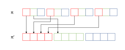
Figure 1: Example of shuffle operation on permutation $\pi$, with $u=3$

By combining shift and shuffle we increase the size of the explored neighborhood, at no extra asymptotic running time cost for the local search implementations.

Local search algorithms that explore shift or shift+shuffle neighborhoods could potentially be stuck in the arbitrarily bad local optimum, following the same argument as in Theorem 6.

If we allow applying shift simultaneously to both $\mathbf{x}$ and $\mathbf{y}$ we will consider all $mn$ neighbors of the current solution, precisely as in equivalence class example from Section 2. We will call this dual shift neighborhood of a solution $(\mathbf{x},\mathbf{y})$. Notice that a local search algorithm that explores this neighborhood reaches a local optimum only after a single iteration, with running time $O(m^{2}n^{2})$.

A much larger optimized shift neighborhood will be defined as follows. For every shift operation on $\mathbf{x}$ we consider all possible assignments of $\mathbf{y}$, and vice versa, for each shift on $\mathbf{y}$ we will consider all possible assignments of $\mathbf{x}$. Just like in the case of optimized $h$-exchange, this neighborhood is exponential in size, but can be efficiently explored in $O(mn^{3})$ running time by solving corresponding linear assignment problems.

Theorem 12.

For local search based on dual shift and optimized shift neighborhoods, the final solution value is guaranteed to be no worse than $\mathcal{A}(Q,C,D)$.

Proof.

The proof for dual shift neighborhood follows from the fact that we are completely exploring the equivalence class defined by $\sim$ of a given solution, as in Theorem 2.

For optimized shift, notice that for each shift on one side of $(\mathbf{x},\mathbf{y})$ we consider all possible solutions on the other side. This includes all possible shifts on that respective side. Therefore the set of solutions of optimized shift neigborhood includes the set of solutions of dual shift neighborhood, and contains the solution with the value at most $\mathcal{A}(Q,C,D)$. ∎

In [9] we have explored the complexity of a special case of BAP where $Q$, observed as a $m^{2}\times n^{2}$ matrix, is restricted to be of a fixed rank. The rank of such $Q$ is said to be at most $r$ if and only if there exist some $m\times m$ matrices $A^{{}^{p}}=(a_{ij}^{p})$ and $n\times n$ matrices $B^{{}^{p}}=(b_{ij}^{p})$, $p=1,\ldots,r,$ such that

$$q_{ijkl}=\sum_{p=1}^{r}a_{ij}^{p}b_{kl}^{p}$$ (19)

for all $i,j\in M$, $k,l\in N$.

Theorem 13.

Alternating Algorithm and local search algorithms that explore optimized $h$-exchange and optimized shift neighborhoods will find an optimal solution to BAP $(Q,C,D)$, if $Q$ is a non-negative matrix of rank $1$, and both $C$ and $D$ are zero matrices.

Proof.

Note that in the case described in the statement of the theorem, we are looking for such $(\mathbf{x}^{*},\mathbf{y}^{*})$ that minimizes $(\sum_{i,j=1}^{m}a_{ij}x^{*}_{ij})\cdot(\sum_{k,l=1}^{n}b_{kl}y^{*}_{kl})$, where $q_{ijkl}=a_{ij}b_{kl},\,\forall i,j\in M,\,k,l\in N$. If we are restricted to non-negative numbers, solutions to corresponding linear assignment problems would be an optimal solution to this BAP. It is easy to see that, for any fixed $\mathbf{x}$, a solution of the smallest value will be produced by $\mathbf{y}^{*}$. And viceversa, for any fixed $\mathbf{y}$, a solution of the smallest value will be produced by $\mathbf{x}^{*}$.

Optimized $h$-exchange neighborhood, optimized shift neighborhood and the neighborhood that Alternating Algorithm is based on, all contain the solution that has one side of $(\mathbf{x},\mathbf{y})$ unchanged and has the optimal assignment on the other side. Therefore, the local search algorithms that explore these neighborhoods will proceed to find optimal $(\mathbf{x}^{*},\mathbf{y}^{*})$ in at most $2$ iterations. ∎

5 Experimental design and test problems

In this section we present general information on the design of our experiments and generation of test problems.

All experiments are conducted on a PC with Intel Core i7-4790 processor, 32 GB of memory under control of Linux Mint 17.3 (Linux Kernel 3.19.0-32-generic) 64-bit operating system. Algorithms are coded using Python 2.7 programming language and run via PyPy 5.3 implementation of Python. The linear assignment problem, that appears as a subproblem for several algorithms, is solved using Hungarian algorithm [21] implementation in Python.

5.1 Test problems

As there are no existing benchmark instances available for BAP, we have created several sets of test problems, which could be used by other researchers in the future experimental analysis. Three categories of problem instances are considered: uniform, normal and euclidean.

• For uniform instances we set $c_{ij},d_{kl}=0$ and the values $q_{ijkl}$ are generated randomly with uniform distribution from the interval $[0,mn]$ and rounded to the nearest integer.

• For normal instances we set $c_{ij},d_{kl}=0$ and the values $q_{ijkl}$ are generated randomly following normal distribution with mean $\mu=\frac{mn}{2}$, standard deviation $\sigma=\frac{mn}{6}$ and rounded to the nearest integer.

• For euclidean instances we generate randomly with uniform distribution four sets of points $A,B,U,V$ in Euclidean plane of size $[0,1.5\sqrt[2]{mn}]\times[0,1.5\sqrt[2]{mn}]$, such that $|A|=|B|=m$, $|U|=|V|=n$. Then $C$ and $D$ are chosen as zero vectors, and $q_{ijkl}=||a_{i}-u_{k}||\cdot||b_{j}-v_{l}||$ (rounded to the nearest integer), where $a_{i}\in A,b_{j}\in B,u_{k}\in U,v_{l}\in V$.

Test problems are named using the convention “type size number”, where type $\in$ {uniform, normal, euclidean}, size is of the form $m\times n$, and number $\in\{0,1,\ldots\}$. For every instance type and size we have generated 10 problems, and all the results of experiments will be averaged over those 10 problems. For example, in a table or a figure, a data point for “uniform $50\times 50$” would be the average among the 10 generated instances. This applies to objective function values, running times and number of iterations, and would not be explicitly mentioned throughout the rest of the paper. Problem instances, results for our final set of experiments as well as best found solutions for every instance are available upon request from Abraham Punnen (apunnen@sfu.ca).

6 Experimental analysis of construction heuristics

In Section 3 we presented several construction approaches to generate a solution to BAP. In this section we discuss results of computational experiments using these heuristics.

The experimental results are summarized in Table 1. For the heuristic GreedyRandomized, we have considered the candidate list size $2$, $4$ and $6$. In the table, columns GreedyRandomized2 and GreedyRandomized4 refer to implementations with candidate list size of $2$ and $4$, respectively. Results for candidate list size $6$ are excluded from the table due to poor performance.

Here and later when presenting computational results, “value” and “time” refer to objective function value and running time of an algorithm. The best solution value among all tested heuristics is shown in bold font. We also report (averaged over 10 instances of given type and size) the average solution value $\mathcal{A}(Q,C,D)$ (denoted simply as $\mathcal{A}$), computed using the closed-form expression from Section 2.

Table 1: Solution value and running time in seconds for construction heuristics

		RandomXYGreedy		Greedy		GreedyRandomized2		GreedyRandomized4		Rounding
instances	$\mathcal{A}$	value	time	value	time	value	time	value	time	value	time
uniform 20x20	79975	62981	0.0011	61930	0.0016	61824	0.0015	62997	0.0023	58587	0.0282
uniform 40x40	1280013	1039365	0.0024	1038410	0.0085	1046862	0.0117	1047444	0.0107	1005375	0.4083
uniform 60x60	6480224	5335157	0.0057	5399004	0.0362	5430190	0.0403	5429077	0.0381	5311287	2.076
uniform 80x80	20480398	17179410	0.0119	17393975	0.0901	17427649	0.1092	17455112	0.1231	17127745	8.6041
uniform 100x100	50001181	42492213	0.0205	43134618	0.1797	43115743	0.1755	43209207	0.2431	42521606	29.3038
uniform 120x120	103680291	88710617	0.0334	90317432	0.2459	90450040	0.3127	90388890	0.3208	89342939	90.1245
uniform 140x140	192079012	165656443	0.0518	168664018	0.404	168695610	0.5922	168683177	0.5869	166927409	196.3766
uniform 160x160	327679690	284623314	0.0768	289819325	0.939	289847112	0.9922	290034508	0.9862	287148038	339.6329
uniform 180x180	524879096	458395075	0.1088	466419210	1.0135	466652862	1.107	466938203	1.5316	462852252	539.6931
normal 20x20	79977	69989	0.0011	69032	0.0013	69322	0.0015	69899	0.0022	67367	0.0275
normal 40x40	1280007	1137550	0.0022	1137478	0.008	1139150	0.0098	1139608	0.0116	1123670	0.3902
normal 60x60	6480142	5825775	0.0055	5847641	0.0229	5841178	0.0277	5860741	0.0427	5795676	2.0257
normal 80x80	20480028	18555962	0.0108	18696934	0.0613	18658585	0.0772	18697475	0.102	18544051	6.9208
normal 100x100	50000062	45647505	0.02	45909621	0.1293	45925799	0.1584	45943220	0.1958	45643447	30.2969
normal 120x120	103680643	94952757	0.0325	95765991	0.2465	95711199	0.2967	95757531	0.3385	95332171	80.9744
normal 140x140	192079732	176656351	0.0507	178279212	0.4034	178238835	0.4936	178233293	0.556	177501940	179.0639
normal 160x160	327681533	302496650	0.0738	305379404	0.746	305333912	0.696	305345983	0.823	304080792	310.9162
normal 180x180	524880349	486132477	0.1056	490345723	0.8888	490464093	1.0742	490656416	1.3211	489077716	540.4644
euclidean 20x20	95297	93756	0.0011	98864	0.0013	99027	0.0014	98104	0.0015	85564	0.0276
euclidean 40x40	1554313	1540492	0.0024	1559829	0.0111	1546894	0.0116	1551881	0.0123	1430068	0.4218
euclidean 60x60	8003105	7821082	0.0063	8021089	0.0445	8014594	0.0461	7945751	0.0489	7331236	1.9805
euclidean 80x80	24906273	24190227	0.0129	24873255	0.0611	24799662	0.0954	24853670	0.0805	23145446	6.141
euclidean 100x100	61053265	59345477	0.0235	60305521	0.103	59882626	0.1285	60052837	0.1223	56848260	31.8484
euclidean 120x120	126198999	121816738	0.0389	123601338	0.2986	123829252	0.305	124053452	0.3252	117754675	93.6024
euclidean 140x140	230673448	221785417	0.0617	227949036	0.4082	227508295	0.4637	227854403	0.4979	214876628	183.0906
euclidean 160x160	404912898	390412111	0.0897	395260253	0.8908	398388924	0.8284	396277525	1.0551	378608021	309.2262
euclidean 180x180	635700756	607470603	0.1289	623035384	1.1913	625456121	1.356	623393649	1.4349	593800828	548.8153

As the table shows, for smaller uniform and normal instances as well as for all euclidean instances Rounding produced better quality results, however, using substantially longer time. For all other problems RandomXYGreedy obtained better results. To our surprise, the quality of the solution produced by Greedy was inferior to that of RandomXYGreedy. It can, perhaps, be explained as a consequence of being “too greedy” in the beginning, leading to worse overall solution, particularly, taking into consideration the quadratic nature of the objective function. In the initial steps the choice is made based on the very much incomplete information about solution and the interaction cost of $\mathbf{x}$ and $\mathbf{y}$ assignments. In addition, the running time for RandomXYGreedy was significantly lower than that of Rounding and other algorithms. Thus, we conclude that RandomXYGreedy is our method of choice if a solution to BAP is needed quickly.

As for the GreedyRandomized strategy, the higher the size of the candidate list, the worse is the quality of the resulting solution. On the other hand, larger sizes of the candidate lists provide us with more diversified ways to generate solutions for BAP. That may have advantages if the construction is followed by an improvement approach as generally done in GRASP algorithm.

In Figures 2 and 3 we present solution value and running time results of this section for uniform instances.

Figure 2: Difference between solution values (to the best) for construction heuristics; uniform instances

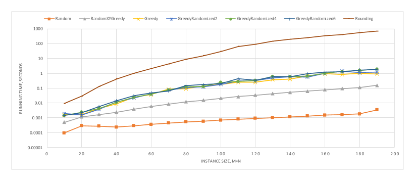
Figure 3: Running time for construction heuristics; uniform instances

7 Experimental analysis of local search algorithms

Let us now discuss the results of computational experiments carried out using local search algorithms that explore neighborhoods discussed in Section 4. All algorithms are started from the same random solution and ran until a local optimum is reached. In addition to the objective function value and running time we report the number of iterations for each approach.

For $h$-exchange neighborhoods, we selected $2$ and $3$-exchange local search algorithms (denoted by 2ex and 3ex) as well as the Alternating Algorithm (AA).

From [$h,p$]-exchange based algorithms, we have implemented $[2,2]$-exchange local search (named Dual2ex). The $[2,2]$-exchange neighborhood can be explored in $O(m^{2}n^{2})$ time, using efficient recomputation of the change in the objective value. We refer to the algorithm that explores optimized $2$-exchange neighborhood as 2exOpt. The running time of each iteration of this local search is $O(m^{2}n^{3})$. To speed up this potentially slow approach, we have also considered a version, namely 2exOptHeuristic, where we use an $O(n^{2})$ heuristic to solve the underlying linear assignment problem, instead of the Hungarian algorithm with cubic running time. The running time of each iteration of 2exOptHeuristic is then $O(m^{2}n^{2})$. Similarly defined will be 3exOpt.

Shift, ShiftShuffle, DualShift and ShiftOpt are implementations of local search based on shift, shift+shuffle, dual shift and optimized shift neighborhoods respectively.

In addition, we consider variations of the above-mentioned algorithms, namely 2exFirst, 3exFirst, Dual2exFirst, 2exOptFirst, 2exOptHeuristicFirst, ShiftOptFirst, where corresponding neighborhoods explored only until the first improving solution is encountered.

We provide a summary of complexity results on these local search algorithms in Table 2. Here by $I$ we denote the number of iterations (or “moves”) that it takes for a corresponding search to converge to a local optimum. As $I$ could potentially be exponential in $n$ and will vary between algorithms, we use this notation to simply emphasize the running time of an iteration of each approach.

Table 2: Asymptotic running time and neighborhood size per iteration for local searches

name	running time	neighborhood size per iteration
2ex	$O(n^{3}+In^{2})$	$\Theta(n^{2})$
Shift	$O(In^{3})$	$n$
ShiftShuffle	$O(In^{3})$	$\Theta(n^{2})$
3ex	$O(In^{3})$	$\Theta(n^{3})$
AA	$O(In^{3})$	$n!$
DualShift	$O(n^{4})$	$n^{2}$
Dual2ex	$O(In^{4})$	$\Theta(n^{4})$
ShiftOpt	$O(In^{4})$	$n\cdot n!$
2exOptHeuristic	$O(In^{4})$	$\Theta(n^{2}\cdot n!)^{*}$
2exOpt	$O(In^{5})$	$\Theta(n^{2}\cdot n!)$
3exOpt	$O(In^{6})$	$\Theta(n^{3}\cdot n!)$
* 2exOptHeuristic does not fully explore the neighborhood.

Table 3 summarizes experimental results for 2ex, 3ex, AA, 2exOpt and 2exOptFirst. Results for other algorithms are not included in the table due to inferior performance. However, figures 4 and 5 provide additional insight into the performance of all the algorithms we have tested, for the case of uniform instances.

Table 3: Solution value, running time in seconds and number of iterations for local searches

		2ex			3ex			AA			2exOpt			2exOptFirst
instances	$\mathcal{A}$	value	time	iter	value	time	iter	value	time	iter	value	time	iter	value	time	iter
uniform 10x10	4995	3378	0.0	9	3241	0.0	9	3385	0.0	3	3103	0.04	4	3128	0.02	11
uniform 20x20	80043	59371	0.0	20	56593	0.01	18	56097	0.01	4	54912	0.68	6	55059	0.34	25
uniform 30x30	404944	310455	0.02	32	297569	0.05	28	298787	0.02	4	291520	3.96	6	291268	3.09	46
uniform 40x40	1279785	1003731	0.04	45	977498	0.14	39	971400	0.06	5	954676	21.71	10	957381	8.46	56
uniform 50x50	3124809	2493822	0.08	57	2433665	0.32	49	2416832	0.13	5	2385232	63.49	11	2389496	24.94	73
uniform 60x60	6479878	5256357	0.15	74	5149634	0.59	55	5098653	0.26	6	5056566	143.48	11	5031368	80.32	97
uniform 70x70	12005619	9844646	0.24	85	9682798	1.1	67	9587489	0.38	6	9469736	326.04	14	9472549	156.78	114
uniform 80x80	20480209	17022523	0.37	96	16694088	1.81	75	16519908	0.66	7	16388545	504.34	12	16355658	285.23	136
uniform 90x90	32803918	27479017	0.52	111	26978715	2.97	88	26650508	1.08	8	26563051	882.81	13	26514860	497.74	158
uniform 100x100	49999078	42138227	0.74	124	41363121	4.96	109	41031842	1.45	8	40912367	1480.03	14	40767754	864.39	172
uniform 110x110	73206906	61988038	1.06	148	61179121	6.57	109	60529975	1.92	7	60162728	2406.29	15	60068824	1504.27	196
uniform 120x120	103679901	88602187	1.23	137	87330165	8.52	109	86174642	2.61	8	85872203	3865.67	18	85670906	1917.76	201
normal 10x10	4999	4044	0.0	10	4019	0.0	9	4040	0.0	2	3910	0.03	4	3862	0.02	14
normal 20x20	79955	67321	0.0	20	66520	0.01	16	66179	0.01	3	64913	0.79	7	65363	0.33	25
normal 30x30	404959	348058	0.02	34	342238	0.06	29	343639	0.03	4	338796	4.98	8	339162	2.61	45
normal 40x40	1279974	1119684	0.04	46	1111127	0.14	33	1099106	0.07	6	1089996	23.21	10	1089752	10.61	60
normal 50x50	3124879	2752326	0.08	63	2737137	0.34	43	2711191	0.14	6	2696287	65.48	11	2696062	32.57	77
normal 60x60	6479794	5769522	0.16	73	5707107	0.7	53	5665027	0.3	7	5640412	151.84	12	5633463	81.97	99
normal 70x70	12004939	10738678	0.24	88	10641129	1.3	65	10596245	0.42	6	10544640	316.24	13	10538513	144.42	116
normal 80x80	20480106	18434378	0.38	103	18282395	2.35	80	18173927	0.71	7	18126933	537.29	12	18095224	338.76	132
normal 90x90	32805972	29736595	0.51	108	29408513	3.79	91	29245481	0.92	6	29176212	1017.08	14	29165974	500.62	151
normal 100x100	49999105	45514117	0.71	122	45009249	5.69	100	44798388	1.45	7	44635991	1602.09	15	44603238	940.19	176
normal 110x110	73205050	66768499	1.01	142	66224593	8.26	110	65812495	2.69	10	65716978	2218.71	13	65539744	1632.32	193
normal 120x120	103681336	95001950	1.32	147	94151507	11.24	116	93702171	2.16	6	93322807	4645.28	20	93248160	2130.64	215
euclidean 10x10	6186	5397	0.0	13	5379	0.0	12	5404	0.0	3	5368	0.05	4	5375	0.03	16
euclidean 20x20	95834	82325	0.01	41	82293	0.01	25	82242	0.01	3	82160	1.27	5	81813	1.52	49
euclidean 30x30	490614	419174	0.02	61	418942	0.07	40	419000	0.03	3	416436	9.13	5	417339	18.19	98
euclidean 40x40	1553544	1314659	0.07	87	1312649	0.21	59	1311131	0.07	3	1309701	37.08	5	1311093	90.91	156
euclidean 50x50	3761359	3178424	0.14	112	3173915	0.5	78	3178006	0.16	4	3167772	134.77	7	3168388	314.91	211
euclidean 60x60	7999029	6740779	0.26	141	6720560	1.04	98	6714400	0.23	4	6714689	314.14	7	6716877	1012.93	296
euclidean 70x70	14909550	12533959	0.45	180	12500249	1.92	117	12490034	0.42	4	12487021	674.66	7	12499281	2354.68	366
euclidean 80x80	25210773	21188706	0.68	200	21182227	3.2	133	21160309	0.55	4	21150070	1222.19	6	21156445	5250.01	456
euclidean 90x90	39495474	33083033	1.04	240	33072079	4.87	145	33082326	0.98	5	33049474	2017.96	6	33089283	10482.75	556

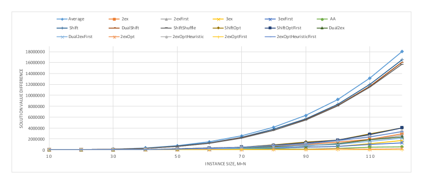
Figure 4: Difference between solution values (to the best) for local search; uniform instances

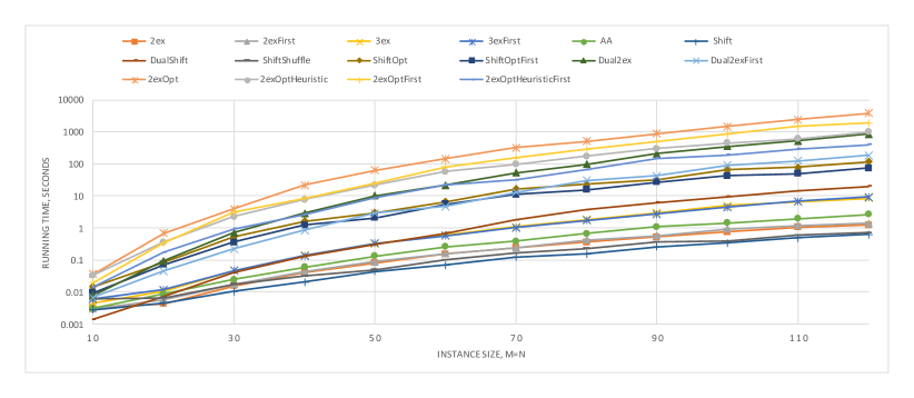
Figure 5: Running time to converge for local search; uniform instances

Even though the convergence speed is very fast for implementations of Shift, ShiftShuffle and DualShift, the resulting solution values are not significantly better than the average value $\mathcal{A}(Q,C,D)$ for the instance.

The optimized shift versions, namely ShiftOpt and ShiftOptFirst produced better solutions but still are outperformed by all remaining heuristics. This fact together with the slower convergence speed (as compared to say 2ex) shows the weaknesses of the approach.

Dual2ex and Dual2exFirst are heavily outperformed both in terms of convergence speed as well as the quality of the resulting solution by AA.

It is also worth mentioning that speeding up 2exOpt and 2exOptFirst by substituting the Hungarian algorithm with an $O(n^{2})$ heuristic for the assignment problem did not provide us with good results. The solution quality decreased substantially and, considering that the running time to converge is still slower than that of AA, we discard these options.

Table 3 presents the results for the better performing set of algorithms. The performance of both first improvement and best improvement approaches 2exFirst, 3exFirst and 2ex, 3ex respectively are similar so we will consider only the latter two from now on. Interestingly, it is not the case for the optimized neighborhoods. We noticed that, for uniform and normal instances 2exOptFirst runs faster than 2exOpt, in most cases. However, for euclidean instances 2exOptFirst takes more time to converge.

As expected, AA is better than 3ex with respect to both solution quality and running time. We will not include any of the $h$-exchange neighborhood search implementations for $h>3$ in this study due to relatively poor performance and huge running time.

We focused the remaining experiments in the paper on 2ex, AA and 2exOpt. Among these 2ex converges the fastest, 2exOpt provides the best solutions and AA assumes a “balanced” position. It is also clear that even better solution quality could be achieved by using implementations of optimized $h$-exchange neighborhood search with higher $h$. However, we show in the next sub-section that this is not feasible in terms of efficient metaheuristics implementation.

7.1 Local search with multi-start

Now we would like to see how well our heuristics perform in terms of solutions quality, when the amount of time is fixed. For this we implemented a simple multi-start strategy for each of the algorithms. The framework will keep restarting the local search from the new Random instance until the time limit is reached. The best solution found in the process is then reported as the result.

Time limit for each instance will be set as the following. Considering the results of the previous sub-section, we expect 3exOptFirst to be the slowest method to converge for all of the instances. We run it exactly once, and use its running time as a time limit for other multi-start algorithms. Together with resulting values we also report the number of restarts of each approach in Table 4. Clearly, the choice of time limit yields $1$ as the number of starts for 3exOptFirst.

Table 4: Solution value and number of starts for time-limited multi-start local searches

		3exOptFirst		2exOpt		2exOptFirst		AA		2ex		2exFirst
instances	time limit	value	starts	value	starts	value	starts	value	starts	value	starts	value	starts
uniform 10x10	0.1	3059	1	2943	3	2974	5	2946	97	2934	221	2980	176
uniform 20x20	2.7	54250	1	53496	4	53286	8	53096	428	53983	997	54244	879
uniform 30x30	23.4	290200	1	288401	5	285630	10	285271	919	292991	1859	292363	1695
uniform 40x40	103.2	948029	1	943982	5	940718	10	936113	1528	963120	2858	960093	2679
uniform 50x50	531.7	2370639	1	2365473	8	2358811	18	2346865	3664	2410678	6592	2401247	6337
uniform 60x60	1148.5	5017422	1	5003247	7	4989212	16	4980930	4221	5105064	7747	5092544	7522
uniform 70x70	3291.3	9429464	1	9421085	10	9404126	21	9369944	7017	9601891	13499	9583585	13009
uniform 80x80	3763.3	16406602	1	16319588	7	16241213	13	16229861	5031	16612105	10017	16583987	9578
normal 10x10	0.1	3857	1	3838	2	3851	5	3828	91	3818	208	3847	162
normal 20x20	2.5	65014	1	64635	4	64433	7	64020	396	64867	902	64738	769
normal 30x30	23.4	337626	1	336552	5	335378	10	335042	899	339448	1818	338849	1623
normal 40x40	113.3	1086083	1	1082094	5	1081530	12	1078755	1675	1092923	3063	1091803	2840
normal 50x50	469.3	2688595	1	2679334	8	2677720	16	2672481	3217	2711913	5807	2704948	5475
normal 60x60	933.4	5640721	1	5627391	6	5612362	13	5604229	3413	5679037	6216	5672749	5979
normal 70x70	3593.3	10512493	1	10492591	12	10483432	25	10474343	7685	10604646	14559	10591133	13903
normal 80x80	11339.0	17989971	1	17993643	20	18010732	42	17995894	15435	18226724	29827	18209532	28425
euclidean 10x10	0.1	5447	1	5430	3	5445	3	5427	98	5427	266	5427	162
euclidean 20x20	5.1	82409	1	81717	4	81710	4	81573	589	81573	1283	81575	747
euclidean 30x30	70.1	418658	1	415529	7	415419	4	414767	2399	414774	3382	414808	1732
euclidean 40x40	390.3	1321385	1	1317439	9	1317948	4	1316409	5459	1316509	6197	1316771	3010
euclidean 50x50	1675.4	3151591	1	3136628	13	3139866	4	3135362	11411	3135723	11993	3136122	5359
euclidean 60x60	4604.9	6563921	1	6532789	15	6537657	4	6529495	17621	6530835	17448	6532247	6641

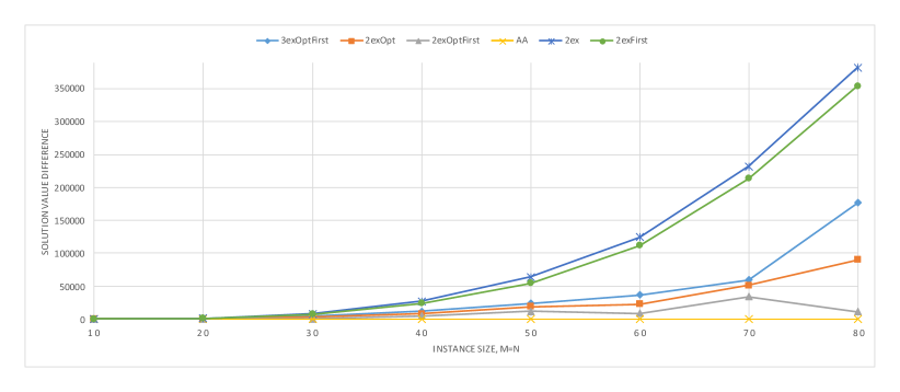
Figure 6: Difference between solution values (to the best) for multi-start algorithms; uniform instances

The best algorithm in these settings is AA, which consistently exhibited better performance for all instance types. The reason behind this is the fact that a local optimum by this approach can be reached almost as fast as by 2ex, however solution quality is much better. On the other hand, the convergence of 2exOpt to a local optimum is very time consuming, and perhaps a better strategy is to do more restarts with slightly less quality of resulting solution. Similar argument holds for the case why 2exOptFirst outperforms 3exOptFirst in this type of experiments. This observation is in contrast with the results experienced by researches of bipartite unconstrained binary quadratic program [15] and bipartite quadratic assignment problem [26]. The difference can be attributed to the more complex structure of BAP in comparison to problems mentioned above.

8 Variable neighborhood search

Variable neighborhood search (VNS) is an algorithmic paradigm to enhance standard local search by making use of properties (often complementary) of multiple neighborhoods [3, 16]. The $2$-exchange neighborhood is very fast to explore and optimized $2$-exchange is more powerful but searching through it for an improving solution takes significantly more time. The neighborhood considered in the Alternating Algorithm works better when significant asymmetry is present regarding $\mathbf{x}$ and $\mathbf{y}$ variables. Motivated by these complementary properties, we have explored VNS based algorithms to solve BAP.

We start by attempting to improve the convergence speed of AA by the means of the faster 2ex. The first variation, named 2ex+AA will first apply 2ex to Random starting solution and then apply AA to the resulting solution. A more complex approach 2exAAStep (Algorithm 4) will start by applying 2ex and as soon as the search converge it will apply a single improvement (step) with respect to Alternating Algorithm neighborhood. After successful update the procedure defaults to running 2ex again. The process stops when no more improvements by AA (and consequently by 2ex) are possible.

Algorithm 4 $2exAAStep$

integers $m,n$; $m\times m\times n\times n$ array $Q$; feasible solution $(\mathbf{x},\mathbf{y})$ to given BAP

feasible solution to given BAP

while True do

    $(\mathbf{x},\mathbf{y})\leftarrow 2ex(m,n,Q,(\mathbf{x},\mathbf{y}))$ $\triangleright$ running $2$-exchange local search (Section 4.1)

    $e_{ij}\leftarrow\sum_{k,l\in N}q_{ijkl}y_{kl}\,\forall i,j\in M$

    $\mathbf{x}^{*}\leftarrow arg\,min_{\mathbf{x}^{\prime}\in\mathcal{X}}\sum_{i,j\in M}e_{ij}x^{\prime}_{ij}$ $\triangleright$ solving assignment problem for $\mathbf{x}$

    if $f(\mathbf{x}^{*},\mathbf{y})<f(\mathbf{x},\mathbf{y})$  then

       continue $\triangleright$ restarting the procedure while loop

    end if

    $g_{kl}\leftarrow\sum_{i,j\in M}q_{ijkl}x^{*}_{ij}\,\forall k,l\in N$

    $\mathbf{y}^{*}\leftarrow arg\,min_{\mathbf{y}^{\prime}\in\mathcal{Y}}\sum_{k,l\in N}g_{kl}y^{\prime}_{kl}$ $\triangleright$ solving assignment problem for $\mathbf{y}$

    if $f(\mathbf{x}^{*},\mathbf{y}^{*})=f(\mathbf{x},\mathbf{y})$  then

       break $\triangleright$ algorithm converged, terminate

    end if

    $\mathbf{x}\leftarrow\mathbf{x}^{*};\,\mathbf{y}\leftarrow\mathbf{y}^{*}$

end while

return ($\mathbf{x}$, $\mathbf{y}$)

Results in Table 5 follow the structure of experimental results reported earlier in the paper. The number of iterations that we report for 2exAAStep is the number of times the heuristic switches from $2$-exchange neighborhood to the neighborhood of the Alternating Algorithm. Clearly, this number will be $1$ for 2ex+AA by design.

Table 5: Solution value, running time in seconds and number of iterations for Alternating Algorithm and variations (convergence to local optima)

	AA		2ex+AA		2exAAStep
instances	value	time	value	time	value	time	iter
uniform 10x10	3255	0.0	3305	0.0	3322	0.01	1
uniform 20x20	56287	0.01	56136	0.01	56076	0.01	3
uniform 30x30	297819	0.02	298485	0.03	297874	0.05	4
uniform 40x40	965875	0.06	967373	0.08	971010	0.13	5
uniform 50x50	2415720	0.11	2414279	0.18	2419385	0.34	6
uniform 60x60	5077348	0.23	5089275	0.33	5095460	0.77	9
uniform 70x70	9578626	0.32	9561747	0.51	9549687	1.25	10
uniform 80x80	16505833	0.59	16422705	0.93	16474525	1.87	10
uniform 90x90	26650437	0.93	26726070	1.16	26706156	3.04	11
uniform 100x100	41027445	1.12	41001387	1.89	41038180	4.78	14
uniform 110x110	60512662	1.72	60549540	2.37	60508210	6.87	15
uniform 120x120	86397256	2.08	86108044	3.23	86019130	10.47	18
uniform 130x130	119380881	3.02	119421396	4.06	119417016	12.52	16
uniform 140x140	161524589	3.58	161725915	5.6	161535754	16.97	18
uniform 150x150	213377462	5.02	214064556	6.9	213453225	22.48	19
normal 10x10	4037	0.0	3997	0.0	3997	0.0	2
normal 20x20	66006	0.01	66372	0.01	66104	0.01	3
normal 30x30	343319	0.02	342316	0.03	342776	0.05	3
normal 40x40	1096961	0.06	1098741	0.09	1101256	0.17	7
normal 50x50	2712329	0.12	2709929	0.2	2708557	0.38	8
normal 60x60	5668986	0.21	5671907	0.33	5678451	0.72	8
normal 70x70	10561145	0.42	10588835	0.57	10581535	1.29	10
normal 80x80	18172093	0.51	18160338	0.87	18141092	2.22	12
normal 90x90	29222387	0.91	29231041	1.3	29283340	2.84	10
normal 100x100	44751122	1.31	44735031	1.72	44753417	5.22	15
normal 110x110	65809366	1.64	65817524	2.39	65812802	6.97	15
normal 120x120	93529513	2.26	93491028	3.58	93581308	8.65	14
normal 130x130	129150096	3.26	129310194	4.14	129238943	12.84	17
normal 140x140	174245361	3.75	174296950	5.91	174169032	20.14	21
normal 150x150	230484514	4.28	230242366	7.32	230292305	24.21	21
euclidean 10x10	5032	0.0	5015	0.0	5015	0.01	1
euclidean 20x20	81714	0.01	81701	0.01	81701	0.01	2
euclidean 30x30	424425	0.03	424261	0.04	424261	0.06	3
euclidean 40x40	1331726	0.06	1330070	0.11	1330070	0.15	4
euclidean 50x50	3342515	0.13	3337157	0.24	3337157	0.35	4
euclidean 60x60	6637101	0.24	6622844	0.42	6622844	0.63	5
euclidean 70x70	12373648	0.33	12345122	0.7	12345122	1.01	4
euclidean 80x80	21088451	0.55	21060424	1.01	21060424	1.34	3
euclidean 90x90	33842019	0.85	33831315	1.48	33831315	2.01	4
euclidean 100x100	50386904	1.08	50351081	2.19	50350547	3.33	5

As all these approaches are guaranteed to be locally optimal with respect to Alternating Algorithm neighborhood, we expect the solution values to be similar. This can be seen in the table. A main observation here is that the 2ex heuristic does not combine well with AA. Increased running time for both 2ex+AA and 2exAAStep confirms that AA is more efficient in searching its much larger neighborhood.

We then explored the effect of combining 2exOptFirst and AA. An algorithm that first runs AA once and then applies 2exOptFirst until convergence will be referred to as AA+2exOptFirst. A more desirable variable neighborhood search based on the discussed heuristics will use the fact that most of the time running AA until convergence is faster than even a single update of the solutions during the 2exOptFirst run. The algorithm AA2exOptFirstStep (Algorithm 5) will use AA to reach its local optimum and then will try to escape it by applying a single first possible improvement of the slower search 2exOptFirst. If successful, the process will start from the beginning with AA. We will also add to the comparison variation with best improvement rule, namely AA2exOptStep.

Algorithm 5 $AA2exOptFirstStep$

integers $m,n$; $m\times m\times n\times n$ array $Q$; feasible solution $(\mathbf{x},\mathbf{y})$ to given BAP

feasible solution to given BAP

while True do

    $(\mathbf{x},\mathbf{y})\leftarrow AA(m,n,Q,(\mathbf{x},\mathbf{y}))$ $\triangleright$ running Alternating Algorithm (Section 4.1)

    for all $i_{1}\in M$ and all $i_{2}\in M\setminus\{i_{1}\}$ do

       $j_{1}\leftarrow$ assigned index to $i_{1}$ in $\mathbf{x}$

       $j_{2}\leftarrow$ assigned index to $i_{2}$ in $\mathbf{x}$

       $\mathbf{x}^{*}\leftarrow\mathbf{x}$

       $x^{*}_{i_{1}j_{1}}\leftarrow 0;\,x^{*}_{i_{2}j_{2}}\leftarrow 0;\,x^{*}_{i_{1}j_{2}}\leftarrow 1;\,x^{*}_{i_{2}j_{1}}\leftarrow 1$ $\triangleright$ applying 2-exchange

       $g_{kl}\leftarrow\sum_{i,j\in M}q_{ijkl}x^{*}_{ij}\,\forall k,l\in N$

       $\mathbf{y}^{*}\leftarrow arg\,min_{\mathbf{y}^{\prime}\in\mathcal{Y}}\sum_{k,l\in N}g_{kl}y^{\prime}_{kl}$ $\triangleright$ solving assignment problem for $\mathbf{y}$

       if $f(\mathbf{x}^{*},\mathbf{y}^{*})<f(\mathbf{x},\mathbf{y})$  then

          $\mathbf{x}\leftarrow\mathbf{x}^{*};\,\mathbf{y}\leftarrow\mathbf{y}^{*}$

          continue while $\triangleright$ restarting the procedure while loop

       end if

    end for

    for all $k_{1}\in N$ and all $k_{2}\in N\setminus\{k_{1}\}$ do

       $l_{1}\leftarrow$ assigned index to $k_{1}$ in $\mathbf{y}$

       $l_{2}\leftarrow$ assigned index to $k_{2}$ in $\mathbf{y}$

       $\mathbf{y}^{*}\leftarrow\mathbf{y}$

       $y^{*}_{k_{1}l_{1}}\leftarrow 0;\,y^{*}_{k_{2}l_{2}}\leftarrow 0;\,y^{*}_{k_{1}l_{2}}\leftarrow 1;\,y^{*}_{k_{2}l_{1}}\leftarrow 1$ $\triangleright$ applying 2-exchange

       $e_{ij}\leftarrow\sum_{k,l\in N}q_{ijkl}y^{*}_{kl}\,\forall i,j\in M$

       $\mathbf{x}^{*}\leftarrow arg\,min_{\mathbf{x}^{\prime}\in\mathcal{X}}\sum_{i,j\in M}e_{ij}x^{\prime}_{ij}$ $\triangleright$ solving assignment problem for $\mathbf{x}$

       if $f(\mathbf{x}^{*},\mathbf{y}^{*})<f(\mathbf{x},\mathbf{y})$  then

          $\mathbf{x}\leftarrow\mathbf{x}^{*};\,\mathbf{y}\leftarrow\mathbf{y}^{*}$

          continue while $\triangleright$ restarting the procedure while loop

       end if

    end forbreak $\triangleright$ algorithm converged, terminate

end while

return ($\mathbf{x}$, $\mathbf{y}$)

The results of these experiments are reported in Table 6. Here, we also report the number of iterations for AA2exOptStep and AA2exOptFirstStep, which represents the number of switches from the Alternating Algorithm neighborhood to optimized $2$-exchange neighborhood before the algorithms converge.

Table 6: Solution value, running time in seconds and number of iterations for 2exOpt and variations (convergence to local optima)

	2ExOptFirst		AA+2exOptFirst		AA2exOptStep			AA2exOptFirstStep
instances	value	time	value	time	value	time	iter	value	time	iter
uniform 10x10	3156	0.02	3059	0.01	3054	0.02	2	3059	0.02	3
uniform 20x20	54670	0.35	54877	0.24	54718	0.32	3	54431	0.2	4
uniform 30x30	291902	2.27	294044	1.12	291184	2.64	4	290011	1.17	4
uniform 40x40	948344	9.78	958550	3.29	953938	5.61	3	958215	3.4	3
uniform 50x50	2379856	33.02	2399151	11.15	2392151	16.57	3	2395319	8.08	3
uniform 60x60	5044883	64.73	5026000	36.08	5030618	35.22	3	5026865	20.45	4
uniform 70x70	9479099	168.6	9511756	67.85	9521222	78.27	3	9501548	28.81	3
uniform 80x80	16418360	252.23	16400987	120.41	16390406	132.04	3	16381373	56.49	3
uniform 90x90	26507000	569.45	26499481	229.48	26536687	238.11	3	26546135	113.07	4
uniform 100x100	40753550	878.32	40894844	293.74	40949795	184.26	1	40875653	155.41	3
uniform 110x110	60079399	1539.8	60231687	458.67	60277301	487.4	3	60196421	317.3	4
uniform 120x120	85818278	2120.85	85774789	1090.37	85996522	526.83	2	86070239	306.32	2
uniform 130x130	118773110	3515.46	118967905	1105.4	119034719	827.06	2	119133276	452.11	3
uniform 140x140	160780185	4860.32	160956538	1304.17	161002007	1479.93	3	161113803	764.84	3
uniform 150x150	213525103	5514.74	213372569	538.34	213372569	748.16	1	213372569	553.21	1
normal 10x10	3866	0.02	3895	0.01	3886	0.02	2	3917	0.01	2
normal 20x20	65262	0.3	65137	0.28	65166	0.36	3	65258	0.21	4
normal 30x30	338569	2.9	340096	1.19	340240	1.52	2	340534	0.86	3
normal 40x40	1087006	10.28	1087569	6.04	1090323	6.93	3	1089412	3.46	4
normal 50x50	2695007	26.39	2697747	14.44	2697124	19.13	3	2696860	7.45	3
normal 60x60	5637608	71.64	5639469	34.18	5634802	45.69	4	5638741	18.75	3
normal 70x70	10538891	159.53	10527751	61.85	10524931	80.22	3	10532494	33.81	3
normal 80x80	18102861	292.68	18102161	145.45	18123379	148.5	4	18125319	62.56	3
normal 90x90	29162243	447.82	29167487	166.29	29176575	193.61	3	29167084	102.4	3
normal 100x100	44610176	953.0	44644532	272.9	44626268	376.46	4	44645246	153.74	3
normal 110x110	65589378	1404.23	65635027	561.99	65669769	423.52	3	65646106	233.42	3
normal 120x120	93315766	2071.35	93321138	697.7	93338052	692.75	3	93300933	346.7	3
normal 130x130	128872342	3329.54	129005518	630.07	128978046	784.53	2	129030228	361.45	2
normal 140x140	173877153	4669.47	174004558	1379.7	174104009	857.84	2	174117705	565.83	2
normal 150x150	229879808	6572.92	229985798	2161.19	230286566	1481.59	3	230254077	757.09	3
euclidean 10x10	4988	0.04	4995	0.02	4992	0.02	1	4996	0.02	1
euclidean 20x20	81833	1.46	81644	0.33	81644	0.31	1	81644	0.28	1
euclidean 30x30	424227	17.82	424425	1.63	424425	1.65	1	424425	1.64	1
euclidean 40x40	1330114	84.25	1331592	7.63	1331592	7.28	1	1331592	7.24	1
euclidean 50x50	3344106	347.38	3342208	22.61	3342208	20.49	1	3342208	18.78	1
euclidean 60x60	6628784	968.15	6637101	43.81	6637101	43.91	1	6637101	43.81	1
euclidean 70x70	12343342	2404.75	12373648	90.12	12373648	90.34	1	12373648	90.1	1
euclidean 80x80	21098260	5579.32	21088451	174.46	21088451	174.94	1	21088451	174.98	1
euclidean 90x90	33892498	11440.65	33841998	333.66	33841998	338.05	1	33841998	326.42	1
euclidean 100x100	50313528	19808.73	50386904	514.2	50386904	515.13	1	50386904	514.74	1

We have noticed that incorporating Alternating Algorithm into optimized 2-exchange yields a much better performance, bringing the convergence time down by at least an order of magnitude. Among variations, AA2exOptFirstStep is consistently faster for uniform and normal instances. However, for euclidean instances performance of all variable neighborhood search algorithms is similar. In fact, for euclidean instances of all sizes the average number of switches between neighborhoods is $1$, which implies that there is no possible improvement from the optimized $2$-exchange neighborhood after the Alternating Algorithm has converged. Thus, the special structure of instances must be always considered when developing metaheuristics for BAP.

Results on convergence time for all described algorithms from this sub-section, for uniform instances, are given in Figure 7.

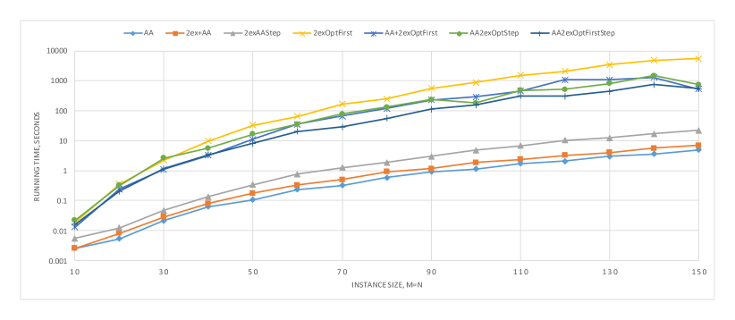
Figure 7: Running time to reach the local optima by algorithms; uniform instances

Our concluding set of experiments is dedicated to finding the most efficient combination of variable neighborhood search strategies and construction heuristics. We consider a variation of the VNS approach with the best convergence speed performance - AA2exOptFirstStep. Namely, let h-AA2exOptFirstStep be the algorithm that first generates $h$ starting solution, using RandomXYGreedy strategy. It then proceeds to apply AA to each of these solutions, selecting the best one and discarding the rest. After that h-AA2exOptFirstStep will follow the description of AA2exOptFirstStep (Algorithm 5) and will alternate between finding an improving solution using optimized $2$-exchange neighborhood and applying AA, until the convergence to local optima. In this sense, AA2exOptFirstStep and 1-AA2exOptFirstStep are equivalent implementations.

The single iteration of AA requires $O(n^{3})$ running time, whereas, a full exploration of the optimized $2$-exchange neighborhood will take $O(m^{2}n^{3})$. From the experiments in Section 7 we also know that it usually takes AA less than 10 iterations to converge. Based on these observations, for the following experimental analysis we have chosen $h$ for h-AA2exOptFirstStep as $h\in\{4,10,100\}$.

In addition to versions of h-AA2exOptFirstStep we consider a simple multi-start AA strategy that performed well in previous experiments (see Section 7.1), denoted msAA. Now however, the starting solution each time is generated using RandomXYGreedy construction heuristic. As the time limit for this multi-start approach we select the highest convergence time among all h-AA2exOptFirstStep variations. As it often happens during the time-limited multi-start procedures, the best solution will be found before the final iteration. Hence, in addition to the total number we also report the average iteration (best iter) at which the finally reported solution was found, and the standard deviation of this value.

See the results of these experiments in Table 7 and Figure 8.

Table 7: Solution value, running time in seconds and number of iterations for Variable Neighborhood Search and multi-start AA

	AA2ExOptFirstStep			4AA2ExOptFirstStep			10AA2ExOptFirstStep			100AA2ExOptFirstStep			msAA
instances	value	time	iter	value	time	iter	value	time	iter	value	time	iter	value	time	iter	best iter	$\sigma(\text{best iter})$
uniform 10x10	3162	0.02	3	3126	0.01	1	3025	0.01	1	2983	0.06	1	2995	0.07	116	47	41
uniform 20x20	55131	0.15	2	54601	0.17	2	54294	0.19	2	53281	0.58	1	53620	0.59	131	54	37
uniform 30x30	293385	0.89	3	292039	0.83	2	289483	0.92	2	286542	2.42	1	287169	2.44	130	57	49
uniform 40x40	955295	3.03	3	950608	2.77	3	951947	2.87	2	942849	6.82	1	939052	6.85	138	89	32
uniform 50x50	2380817	11.35	5	2379835	11.88	4	2375551	7.42	2	2370805	15.35	1	2360529	16.56	165	83	52
uniform 60x60	5038934	19.96	3	5030082	15.28	2	5015756	18.16	2	4990868	35.36	2	4993774	38.42	208	112	35
uniform 70x70	9479825	34.21	4	9436974	43.32	3	9445502	39.85	3	9413893	54.29	1	9399736	61.76	203	115	67
uniform 80x80	16389632	61.47	3	16357168	55.61	2	16303348	59.12	2	16261295	95.21	1	16264848	104.0	217	95	54
uniform 90x90	26505894	110.55	3	26456700	94.5	3	26407075	80.08	1	26356116	151.23	2	26342919	160.45	226	83	64
uniform 100x100	40782492	141.59	3	40712949	180.44	3	40633567	165.63	3	40540438	208.3	1	40506423	241.3	241	116	96
uniform 120x120	85825930	342.18	3	85579139	274.87	2	85471530	333.39	3	85335239	441.49	1	85283242	509.31	273	122	71
uniform 140x140	160605657	693.67	3	160415349	555.54	3	160292924	474.41	1	160035009	719.05	1	159912990	927.88	286	131	124
uniform 160x160	277129402	909.79	2	276565751	918.66	2	276159588	908.23	2	275721038	1386.9	1	275725334	1657.71	302	154	100
normal 10x10	3894	0.02	3	3855	0.01	2	3855	0.01	1	3808	0.07	1	3809	0.07	117	40	37
normal 20x20	65712	0.15	2	65077	0.17	2	64803	0.2	1	64293	0.58	1	64477	0.58	130	73	48
normal 30x30	338547	1.17	5	337693	0.95	3	338138	0.79	1	335113	2.75	2	335756	2.76	145	74	42
normal 40x40	1090670	2.81	3	1088357	3.1	3	1085519	2.69	2	1081375	7.56	1	1082915	7.58	154	81	46
normal 50x50	2696368	8.24	3	2692035	8.33	2	2682121	8.66	3	2678345	17.52	2	2680271	17.58	175	71	55
normal 60x60	5647247	17.06	3	5633194	14.77	1	5627675	17.07	2	5616899	31.56	2	5617125	32.18	173	83	55
normal 70x70	10549768	26.89	1	10519922	34.7	3	10509205	30.19	2	10493809	57.37	2	10494503	61.86	201	104	64
normal 80x80	18095404	72.05	3	18069406	59.64	2	18067347	55.46	2	18032081	86.61	1	18023497	100.11	209	112	62
normal 90x90	29115217	107.77	3	29103538	103.37	2	29097191	95.29	2	29045978	165.73	2	29027250	187.3	264	120	71
normal 100x100	44618697	130.7	2	44578918	138.0	2	44556729	162.61	3	44484747	245.72	3	44482231	279.76	274	172	62
normal 120x120	93293438	343.2	3	93162243	313.92	2	93112300	309.4	2	93023046	506.08	2	92984865	540.0	282	149	93
normal 140x140	173820624	535.5	2	173653510	510.49	2	173594266	481.53	1	173434718	815.2	2	173430869	900.03	279	144	76
normal 160x160	298434202	967.33	2	297840806	899.65	2	297816150	1030.84	2	297540220	1211.89	1	297480023	1567.93	294	126	62
euclidean 10x10	5037	0.02	1	5026	0.02	1	5027	0.02	1	5026	0.11	1	5026	0.11	116	6	7
euclidean 20x20	82675	0.25	1	82008	0.26	1	81842	0.31	1	81718	1.0	1	81718	1.0	129	12	11
euclidean 30x30	411014	1.78	1	408739	1.72	1	407379	1.91	1	406970	4.23	1	406970	4.24	162	32	43
euclidean 40x40	1348302	6.68	1	1342159	6.99	1	1339683	7.09	1	1337792	12.69	1	1337738	12.72	204	48	58
euclidean 50x50	3231060	21.05	1	3219207	20.39	1	3214867	19.94	1	3210442	30.74	1	3210280	31.97	254	37	36
euclidean 60x60	6548901	44.42	1	6519075	44.82	1	6515800	46.24	1	6507833	65.26	1	6507813	65.41	304	32	23
euclidean 70x70	12315235	93.93	1	12283239	100.51	1	12264197	96.28	1	12257619	126.03	1	12256435	128.94	388	74	76
euclidean 80x80	21240164	187.89	1	21143316	183.3	1	21104571	185.35	1	21096255	229.53	1	21095365	232.0	459	144	132
euclidean 90x90	33385322	335.48	1	33323860	319.99	1	33296502	326.28	1	33279588	388.9	1	33277417	398.29	558	81	126
euclidean 100x100	51524424	530.7	1	51382552	535.98	1	51303227	538.1	1	51289100	632.49	1	51286565	633.16	597	158	133
euclidean 120x120	105192868	1291.27	1	105092433	1284.2	1	105037756	1404.01	1	104969850	1456.4	1	104965462	1556.45	908	93	112

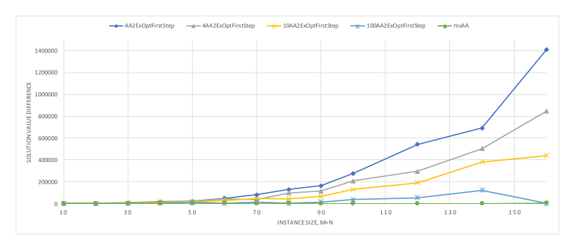
Figure 8: Difference between solution values (to the best) for algorithms; uniform instances

Under this considerations, multi-start AA once again performed the best. h-AA2exOptFirstStep variations were the more efficient, the higher the number $h$ was. Interestingly, for several instance sizes, the average iteration of finding the best solution by msAA is substantially bellow $100$. However, the observed standard deviation is very high, which hints towards the variability of the solutions produced by AA. To confirm this, we present in Figures 9, 10 and 11 the spread of solution values produced by applying AA to the solution of RandomXYGreedy (denoted as RandomXYGreedy+AA). All three instances in these charts are of size $m=n=100$, and we perform $100$ runs of this metaheuristic.

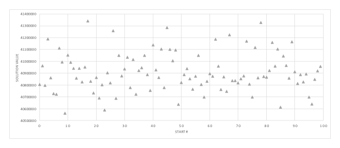
Figure 9: Objective solution values for RandomXYGreedy+AA metaheuristic; uniform $100\times 100$ instance

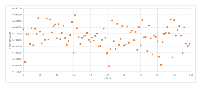
Figure 10: Objective solution values for RandomXYGreedy+AA metaheuristic; normal $100\times 100$ instance

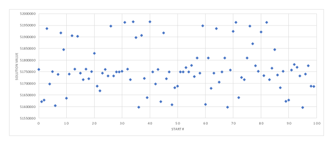
Figure 11: Objective solution values for RandomXYGreedy+AA metaheuristic; euclidean $100\times 100$ instance

At this point, we conclude that optimized $2$-exchange neighborhood is too costly to explore, in comparison to the neighborhood that AA is based on. For the general case it is more effective to do several more restarts of AA from RandomXYGreedy solutions then to spend time escaping local optima with even a single step of 2exOpt. It is suggested to only use efficient implementations of VNS that explore optimized $2$-exchange neighborhood as the final step of any metaheuristic. In this way you can improve your solution quality without excessive time spending, while leaving all the heavy work for Alternation Algorithm.

Our previous experiments that involve multi-start strategies (in this section and Section 7.1) have reasonable time limit restrictions. This considerations are important when developing algorithms to run on real-life instances. However, we are also interested in behavior of multi-start AA and multi-start VNS in the case of unlimited (or unreasonably large) running time constraints. Figure 12 presents results of running multi-start AA, multi-start 1-AA2exOptFirstStep and multi-start 100-AA2exOptFirstStep, for a single $100\times 100$ uniform instance, for an exceedingly long period of time. All starts are made from the solutions generated by RandomXYGreedy heuristic. Here we report the change of the best found solution value, depending on time.

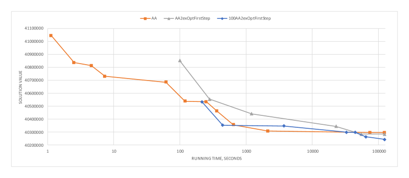
Figure 12: Improvement over time of best found objective solution value for multi-start heuristics; uniform $100\times 100$ instance

We can see that after 50000 seconds (0.58 days of running) multi-start VNS strategies begin to dominate the multi-start AA, even though the later approach is much more efficient in solution space exploration for short running times. This observation is consistent with optimized $h$-exchange being a more powerful neighborhood in terms of solutions quality.

9 Conclusion

We have presented the first systematic experimental analysis of heuristics for BAP along with some theoretical results on local search algorithms worst case performance.

Three classes of neighborhoods - $h$-exchange, $[h,p]$-exchange and shift based - are introduced. Some of the neighborhoods are of an exponential size but can be searched for an improving solution in polynomial time. Analysis of local optimums in terms of domination properties and relation to average value $\mathcal{A}(Q,C,D)$ are presented.

Several greedy, semi-greedy and rounding construction heuristics are proposed for generating reasonable quality solution quickly. Experimental results show that RandomXYGreedy is a good alternative among the approaches. The built-in randomized decision steps make this heuristic valuable for generating starting solutions for improvement algorithms within a multistart framework.

Extensive computational analysis has been carried out on the searches based on described neighborhoods. The experimental results suggest that the very large-scale neighborhood (VLSN) search algorithm - Alternating Algorithm (AA), when used within multi-start framework, yields a more balanced heuristic in terms of running time and solution quality. A variable neighborhood search (VNS) algorithm, that strategically uses optimized $2$-exchange neighborhood and AA neighborhood, produced superior outcomes. However, this came with the downside of a significantly larger computational time.

We hope that this study inspires additional research work on the bilinear assignment model, particularly in the area of design and analysis of exact and heuristic algorithms.

References

- [1] Warren P Adams, Monique Guignard, Peter M Hahn, and William L Hightower. A level-2 reformulation–linearization technique bound for the quadratic assignment problem. European Journal of Operational Research, 180(3):983–996, 2007.
- [2] Ravindra K Ahuja, Özlem Ergun, James B Orlin, and Abraham P Punnen. A survey of very large-scale neighborhood search techniques. Discrete Applied Mathematics, 123(1):75–102, 2002.
- [3] Ravindra K Ahuja, Özlem Ergun, James B Orlin, and Abraham P Punnen. Very large-scale neighborhood search: Theory, algorithms, and applications. Handbook of Approximation Algorithms and Metaheuristics, 10, 2007.
- [4] Eric Angel and Vassilis Zissimopoulos. On the quality of local search for the quadratic assignment problem. Discrete Applied Mathematics, 82(1-3):15–25, 1998.
- [5] Rainer Burkard, Mauro Dell’Amico, and Silvano Martello. Assignment problems: revised reprint. SIAM, 2012.
- [6] Rainer E Burkard, Eranda Cela, Günter Rote, and Gerhard J Woeginger. The quadratic assignment problem with a monotone anti-monge and a symmetric toeplitz matrix: Easy and hard cases. Mathematical Programming, 82(1):125–158, 1998.
- [7] Eranda Cela. The quadratic assignment problem: theory and algorithms, volume 1. Springer Science & Business Media, 2013.
- [8] Ante Ćustić and Abraham P Punnen. Average value of solutions of the bipartite quadratic assignment problem and linkages to domination analysis. Operations Research Letters, 45(3):232–237, 2017.
- [9] Ante Ćustić, Vladyslav Sokol, Abraham P Punnen, and Binay Bhattacharya. The bilinear assignment problem: complexity and polynomially solvable special cases. Mathematical Programming, pages 1–21, 2017.
- [10] Thomas A Feo and Mauricio GC Resende. A probabilistic heuristic for a computationally difficult set covering problem. Operations Research Letters, 8(2):67–71, 1989.
- [11] Dmitri G Fon-Der-Flaass. Arrays of distinct representatives—a very simple np-complete problem. Discrete Mathematics, 171(1-3):295–298, 1997.
- [12] Alan M Frieze. Complexity of a 3-dimensional assignment problem. European Journal of Operational Research, 13(2):161–164, 1983.
- [13] Alan M Frieze, J Yadegar, S El-Horbaty, and D Parkinson. Algorithms for assignment problems on an array processor. Parallel Computing, 11(2):151–162, 1989.
- [14] Fred Glover and Abraham P Punnen. The travelling salesman problem: new solvable cases and linkages with the development of approximation algorithms. Journal of the Operational Research Society, 48(5):502–510, 1997.
- [15] Fred Glover, Tao Ye, Abraham P Punnen, and Gary Kochenberger. Integrating tabu search and vlsn search to develop enhanced algorithms: A case study using bipartite boolean quadratic programs. European Journal of Operational Research, 241(3):697–707, 2015.
- [16] Pierre Hansen, Nenad Mladenović, Raca Todosijević, and Saïd Hanafi. Variable neighborhood search: basics and variants. EURO Journal on Computational Optimization, pages 1–32, 2016.
- [17] J Pirie Hart and Andrew W Shogan. Semi-greedy heuristics: An empirical study. Operations Research Letters, 6(3):107–114, 1987.
- [18] Daniel Karapetyan and Abraham P Punnen. Heuristic algorithms for the bipartite unconstrained 0-1 quadratic programming problem. arXiv preprint arXiv:1210.3684, 2012.
- [19] L Kaufman and Fernand Broeckx. An algorithm for the quadratic assignment problem using bender’s decomposition. European Journal of Operational Research, 2(3):207–211, 1978.
- [20] Hiroshi Konno. Maximizing a convex quadratic function over a hypercube. Journal of the Operations Research Society of Japan, 23(2):171–189, 1980.
- [21] Harold W Kuhn. The hungarian method for the assignment problem. Naval Research Logistics Quarterly, 2(1-2):83–97, 1955.
- [22] Eugene L Lawler. The quadratic assignment problem. Management Science, 9(4):586–599, 1963.
- [23] Panos M Pardalos, Henry Wolkowicz, et al. Quadratic Assignment and Related Problems: DIMACS Workshop, May 20-21, 1993, volume 16. American Mathematical Soc., 1994.
- [24] William P Pierskalla. Letter to the editor-the multidimensional assignment problem. Operations Research, 16(2):422–431, 1968.
- [25] Abraham P Punnen, Piyashat Sripratak, and Daniel Karapetyan. Average value of solutions for the bipartite boolean quadratic programs and rounding algorithms. Theoretical Computer Science, 565:77–89, 2015.
- [26] Abraham P Punnen and Yang Wang. The bipartite quadratic assignment problem and extensions. European Journal of Operational Research, 250(3):715–725, 2016.
- [27] Sartaj Sahni and Teofilo Gonzalez. P-complete approximation problems. Journal of the ACM (JACM), 23(3):555–565, 1976.
- [28] Abdolhamid Torki, Yatsutoshi Yajima, and Takao Enkawa. A low-rank bilinear programming approach for sub-optimal solution of the quadratic assignment problem. European Journal of Operational Research, 94(2):384–391, 1996.
- [29] Louis Y Tsui and Chia-Hao Chang. A microcomputer based decision support tool for assigning dock doors in freight yards. Computers & Industrial Engineering, 19(1-4):309–312, 1990.
- [30] Louis Y Tsui and Chia-Hao Chang. An optimal solution to a dock door assignment problem. Computers & Industrial Engineering, 23(1-4):283–286, 1992.