Sensitive and Nonlinear Far Field RF Energy Harvesting in Wireless Communications

Abstract

This work studies both limited sensitivity and nonlinearity of far field RF energy harvesting observed in reality and quantifies their effect, attempting to fill a major hole in the simultaneous wireless information and power transfer (SWIPT) literature. RF harvested power is modeled as an arbitrary nonlinear, continuous, and non-decreasing function of received power, taking into account limited sensitivity and saturation effects. RF harvester’s sensitivity may be several dBs worse than communications receiver’s sensitivity, potentially rendering RF information signals useless for energy harvesting purposes. Given finite number of datapoint pairs of harvested (output) power and corresponding input power, a piecewise linear approximation is applied and the statistics of the harvested power are offered, as a function of the wireless channel fading statistics. Limited number of datapoints are needed and accuracy analysis is also provided. Case studies include duty-cycled (non-continuous), as well as continuous SWIPT, comparing with industry-level, RF harvesting. The proposed approximation, even though simple, offers accurate performance for all studied metrics. On the other hand, linear models or nonlinear-unlimited sensitivity harvesting models deviate from reality, especially in the low-input-power regime. The proposed methodology can be utilized in current and future SWIPT research.

I Introduction

Far field radio frequency (RF) energy harvesting, i.e., the capability of wireless nodes to scavenge energy, either from remote ambient or dedicated RF sources, has recently attracted significant attention. Compared to other energy harvesting methods, e.g., from motion, sun or heat, RF energy harvesting offers the advantage of simultaneous wireless information and power transfer (SWIPT). The latter lies at the heart of the radio frequency identification (RFID) industry, which is expected to drive research and innovation in a plethora of coming Internet-of-Things (IoT) scenarios and low-power applications [1].

Recent SWIPT literature within the wireless communications theory research community has addressed problems relevant to protocol architecture, as well as fundamental performance metrics. Several motivating examples demonstrating the concept of SWIPT exist in the literature, e.g., for memoryless point-to-point channels [2], frequency-selective channels [3], multiple-input multiple-output (MIMO) broadcasting [4], and relaying [5]. For instance, work in [5] studied protocols that split time or power among the RF energy harvesting and information transfer modules within a radio terminal, so that specific communication tasks are performed, while the radio terminal is solely powered by the receiving RF. Wireless power transfer in wireless communications imposes additional energy harvesting constraints [6]. Work in [7] offered several resource allocation algorithms for wideband RF harvesting systems. The reviews in [8, 9] offer the current perspective of linear RF harvesting within the wireless communications theory community.

On the other hand, RF energy harvesting suffers from limited available density issues, typically in the sub-microWatt regime (e.g., work in [10] reports $0.1\mu$Watt/cm² from cellular GSM base stations), in sharp contrast to other ambient energy sources based on sun, motion or electrochemistry; such limited RF density can power only ultra-low-power devices in continuous (non-duty-cycled) operation or low-power devices, such as low-power wireless sensors in delay-limited, duty-cycled operation, since sufficient RF energy must be harvested before operation. That is due to the fact that the far field RF power decreases at least quadratically with distance, while RF harvesting circuits have limited sensitivity, i.e., offer no output when input power is below a threshold, as well as efficiency. A common, critical component of the far field RF harvesting circuits is the rectenna, i.e., the antenna and the rectifier that converts the input RF signal to DC voltage.

The rectifier circuit is typically implemented with one or multiple diodes, imposing strong nonlinearity on the power conversion. In addition, the rectifier circuit has usually three operation regimes, stemming directly from the presence of diodes. First, for input power below the sensitivity of the harvester (i.e., the minimum power for harvesting operation), the harvested power is zero. Second, for input power between sensitivity and saturation threshold (the power level above which the output harvesting power saturates), the harvested power is a continuous, nonlinear, increasing function of input RF power, with response depending on the operating frequency and the circuit components of the rectifier. Lastly, for input power above saturation, the output power of the harvester is saturated. The above three characteristic regimes are depicted in Fig. 1, with the black-dashed line curve, which adhere to a variety of circuits in the microwave literature [13, 14, 15, 16, 17]. The nonlinearity of harvested power as a function of input power is also corroborated by the fact that the conversion efficiency in the microwave circuits literature is always referenced to a specific level of input power.

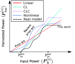
Figure 1: Harvested power vs. input power. For the real rectenna model, the harvested power is an increasing function of input power, taking into account the effect of harvester’s sensitivity.

There exist few recent SWIPT reports studying nonlinear RF harvesting models, i.e., modeling the harvested power as a specific nonlinear function of the input power. Modeling of the harvesting power as a normalized sigmoid function is proposed in [18, 19, 20, 21, 22], whereas work in [23] models the harvested power as a second order polynomial. These studies examine resource allocation algorithms under nonlinear RF harvesting using convex optimization techniques; however, the adopted nonlinear RF harvested power models do not account for the harvester’s limited sensitivity, i.e., sensitivity threshold is assumed zero and the harvester can output power for any non-negative input power value.

There is an important difference between the communications receiver’s sensitivity and the harvester’s sensitivity (defined above), largely overlooked by a wide portion of SWIPT prior art in wireless communications. The first one is the minimum power threshold above which the receiver can reliably decode signals, with values that depend on the temperature, bandwidth, noise figure of the electronics and the minimum signal-to-noise ratio (SNR). Communication sensitivity ranges from $-140$ dBm (e.g., for low-bandwidth radios such as LoRa [24]) to $-85$ dBm (e.g., higher bandwidth GSM cellphones). On the other hand, the state-of-the-art harvesting sensitivity currently obtains values in the order of $-30$ dBm; unfortunately, the harvester’s sensitivity evolves very slowly as a function of years (slower than Moore’s law), due to the involved semiconductor technology; e.g., passive RFID tags harvester sensitivity (in dBm) has improved by a factor of two every $3.8$ years over a two-decade span [25, Fig. 1]. As a result, there is a non-negligible gap around $55-120$ dB between communications receiver’s and harvester’s sensitivity. This gap indicates that the signals with power around communications sensitivity can be decoded at a SWIPT receiver but cannot be exploited for energy harvesting purposes.

Work in [26] proposed exploitation of peak-to-average power ratio (PAPR), when the power of the emitted signal is spread over multiple tones; the peaky behavior of the multi-tone emitted signal can offer adequate bursts of energy to the rectifier, turning on the diode, even if the average input power is below the harvesters’ sensitivity. Prominent signal examples are multi-sine waveforms [27] or orthogonal frequency-division multiplexing (OFDM) waveforms. Subsequent work [28, 29, 30, 31, 32] optimized amplitudes and phases of the multi-tone waveforms, maximizing the harvested power at the receiver, under flat or frequency-selective channels. Convex optimization techniques were employed, with channel state information (CSI) at the transmitter, PAPR constraints and nonlinear, input-output circuit-based analysis of a single-diode or multiple-diode rectifiers [33, 34]. Experimental measurements [35] demonstrated that the harvesting efficiency of multi-tone systems can be increased by $37\%$ compared to single-tone, within the low-input-power range of $[-28,-19]$ dBm. Although the PAPR property of multi-tone signals can increase the end-to-end harvesting efficiency, the level of the studied input powers was still above $-30$ dBm, while the state-of-the-art RF harvesting sensitivity is currently close to $-35$ dBm [16]. More importantly, the effect of limited RF harvesting sensitivity has not been quantified in the context of SWIPT research.

Therefore, the majority of SWIPT studies within the wireless communications community, to the best of our knowledge, either (a) adhere to a linear model of harvested power as a function of input RF power or (b) do not take explicitly into account the effects of harvester’s limited (and not unlimited) sensitivity; the latter is of vital importance, given the fluctuations of received signal input power due to wireless fading, as well as the fact that the harvester’s sensitivity is finite and several tens of dB worse than communications receiver’s sensitivity.

This work introduces both limited sensitivity and nonlinearity of far field RF energy harvesting observed in reality, attempting to fill a major hole in the SWIPT wireless communications theory community. Two rectifier circuit harvesting efficiency models are examined from the prior art for realistic comparison; the first one is the sensitive rectenna proposed in [16] and the second is the PowerCast module [17]. Three (approximation) baseline harvested power models are compared with the realistic harvested power model, depicted in Fig. 1. The first baseline model called linear (L), is the dominant model of RF harvesting prior art. The other two studied baseline models are called constant-linear (CL) and constant-linear-constant (CLC). Additionally, nonlinear harvesting models with unlimited sensitivity are also studied and compared with the approach of this work. The contributions are summarized below:

• For the first time in the literature, harvested power can be modeled as an arbitrary nonlinear, continuous, and non-decreasing function of the input RF power, taking into account (a) the nonlinear efficiency of realistic rectifier RF harvesting circuits, (b) the zero response of energy harvesting circuit for input power below sensitivity (i.e., limited sensitivity), and (c) the saturation effect of harvested power. The impact of harvester’s limited sensitivity is carefully quantified based on the characteristics of the RF harvesting circuitry and the wireless propagation channel.

• Given the wireless channel fading probability density function (PDF) and datapoint pairs of the harvested (output) power and the corresponding input power, stemming from the specifications of the limited-sensitivity, nonlinear harvesting system, this work offers the PDF and cumulative distribution function (CDF) of the harvested power. The offered statistics are based on a piecewise linear approximation. It is also shown that approximation accuracy of at least $\epsilon$ can be achieved by at most $\mathcal{O}(\sqrt{1/\epsilon})$ datapoints.

• Three performance metrics are studied: (i) the expected harvested energy at the receiver, (ii) the expected charging time at the receiver (time-switching scenario), and (iii) the probability of successful reception at the interrogator for passive RFID tags (power-splitting scenario). It is shown that the proposed approximation methodology offers exact performance for all studied metrics. In addition, no tuning of any parameter is required. On the other hand, linear RF harvesting modeling results deviate from reality, and in some cases are off by one order of magnitude, while nonlinear RF harvesting models from recent prior art, that do not take into account limited harvesting sensitivity, deviate from reality in the low-input-power regime.

• The proposed methodology can be applied to any type of RF energy harvesting system, provided that system-level datapoint pairs of the harvested output power and the input power are provided. In that way, accurate SWIPT analysis can be facilitated.

The rest of the document is organized as follows. Section II introduces the channel model, Section III presents the fundamentals of far field RF energy harvesting, explaining the inherent nonlinearity in the real energy harvesting models. Section IV presents the proposed approximation methodology, while Section V compares baseline, linear harvesting models used in prior art with the nonlinear harvesting model, under three performance metrics. Finally, work is concluded in Section VI.

Notation: The set of natural and real numbers is denoted as $\mathds{N}$ and $\mathds{R}$, respectively. For a natural number $N\in\mathds{N}$, set $\{1,2,\ldots,N\}$ is denoted as $[N]\triangleq\{1,2,\ldots,N\}$. Random variables (RVs) are denoted with bold italic letters, e.g., $\boldsymbol{a}$, while vectors are denoted with underlined bold letters, e.g., $\mathbf{\underline{b}}$. Notation $\mathbf{\underline{b}}[j]$ stands for the $j$-th element of vector $\mathbf{\underline{b}}$. Symbol $\odot$ stands for the component-wise (Hadamard) product. Notation $\mathcal{CN}(0,\sigma^{2})$ stands for the circularly-symmetric complex Gaussian distribution of variance $\sigma^{2}$. For a continuous RV $\boldsymbol{a}$, supported over an interval set $\mathcal{X}$, the corresponding PDF and CDF is denoted as $\mathsf{f}_{\boldsymbol{a}}(\cdot)$ and $\mathsf{F}_{\boldsymbol{a}}(x_{0})=\int_{y\in\mathcal{X}:y\leq x_{0}}\mathsf{f}_{\boldsymbol{a}}(y)\mathsf{d}y$, respectively. The expectation and variance of $\mathsf{g}(\boldsymbol{a})$ is denoted as $\underset{}{\mathbb{E}}[\mathsf{g}(\boldsymbol{a})]$ and $\mathsf{var}[\mathsf{g}(\boldsymbol{a})]\triangleq\mathbb{E}[(\mathsf{g}(\boldsymbol{a})-\mathbb{E}[\mathsf{g}(\boldsymbol{a})])^{2}]$, respectively. The Dirac delta function is denoted as $\sDelta(\cdot)$. The probability of event $\mathscr{S}$ is denoted as $\mathbb{P}(\mathscr{S})$ and ${\bf dom}\mathsf{g}$ denotes the domain of function $\mathsf{g}$.

II Wireless System Model

A source of RF signals offers wireless power to an information and far field RF energy harvesting (IEH) terminal. The source of RF signals is assumed with a dedicated power source, while the far field IEH terminal harvests RF energy from the incident signals on its antenna and could operate as information transmitter or receiver.

Narrowband transmissions are considered over a quasi-static flat fading channel. For a single channel use, the downlink received signal at the output of the matched filter at the IEH terminal is given by:

$$\boldsymbol{y}=\sqrt{P_{\rm T}\,T_{\rm s}\,\mathsf{L}(d)}\,\boldsymbol{h}\,\boldsymbol{s}+\boldsymbol{w},$$ (1)

where $\boldsymbol{s}$ is the transmitted symbol, with $\mathbb{E}[\boldsymbol{s}]=0$ and $\mathbb{E}\left[|\boldsymbol{s}|^{2}\right]=1$, $P_{\rm T}$ is the average transmit power of the RF source, $T_{\rm s}$ is the symbol duration, $\boldsymbol{h}$ is the complex baseband channel response, $\mathsf{L}(d)$ is the path-gain (or inverse path-loss) coefficient at distance $d$, and $\boldsymbol{w}\sim\mathcal{CN}(0,\sigma_{\rm d}^{2})$ is the additive white complex Gaussian noise at the IEH receiver.

A block fading model is considered, where the channel response changes independently every coherence block of $T_{\rm c}$ seconds. $\boldsymbol{h}^{(n)}$ denotes the complex baseband channel response at the $n$-th coherence block. At each coherence block, the RF source transmits a packet whose duration spans $T_{\rm p}$ seconds, which in turn spans several symbols, with $T_{\rm p}\leq T_{\rm c}$. The received RF input power (simply abbreviated as input power) at the IEH terminal during the $n$-th coherence time block is given by:

$$\boldsymbol{P}_{\rm R}^{(n)}=\mathbb{E}\!\left[|\boldsymbol{s}|^{2}\right]P_{\rm T}\,\mathsf{L}(d)\,\left|\boldsymbol{h}^{(n)}\right|^{2}=\mathsf{P}(d)\boldsymbol{\gamma}^{(n)},$$ (2)

where $\mathsf{P}(d)\triangleq P_{\rm T}\,\mathsf{L}(d)$ and $\boldsymbol{\gamma}^{(n)}\triangleq\left|\boldsymbol{h}^{(n)}\right|^{2}$. Note that $\boldsymbol{P}_{\rm R}^{(n)}$ is a function of $\boldsymbol{\gamma}^{(n)}$, i.e., $\boldsymbol{P}_{\rm R}^{(n)}\equiv\boldsymbol{P}_{\rm R}^{(n)}(\boldsymbol{\gamma}^{(n)})$. Due to the definition of channel coherence time block, RVs $\left\{\boldsymbol{h}^{(n)}\right\}$ are independent and identically distributed (IID) across different values of $n$. It is also assumed that RVs $\boldsymbol{\gamma}^{(n)}$ are drawn from a continuous distribution, denoted as $\mathsf{f}_{\boldsymbol{\gamma}^{(n)}}(\cdot)$, supported over the non-negative reals, $\mathds{R}_{+}$. Hence, the corresponding distribution of $\boldsymbol{P}_{\rm R}^{(n)}$ has a continuous density in $\mathds{R}_{+}$.

Figure 2: The architecture of far field RF energy harvesters. Typical rectifier circuits with a single diode [16] (upwards) or multiple diodes [36] (downwards) are also depicted, emphasizing in the nonlinear relationship between harvested and input RF power.

The presented results will be offered without having in mind a specific type of fading distribution. For the specific numerical results, Nakagami fading will be considered, since it can describe small-scale wireless fading under both line-of-sight (LoS) or non-line-of-sight (NLoS) scenarios. Under Nakagami distribution, the PDF of $\boldsymbol{\gamma}^{(n)}$ follows Gamma distribution with shape parameters $\left(\mathtt{m},\frac{\Omega}{\mathtt{m}}\right)$, given by:

$$\mathsf{f}_{\boldsymbol{\gamma}^{(n)}}(x)=\left(\frac{\mathtt{m}}{\Omega}\right)^{\mathtt{m}}\,\frac{x^{\mathtt{m}-1}}{\Gamma(\mathtt{m})}\,\mathsf{e}^{-\frac{\mathtt{m}}{\Omega}x},~{}~{}x\geq 0,$$ (3)

where $\Gamma(x)=\int_{0}^{\infty}t^{x-1}\mathsf{e}^{-t}\mathsf{d}t$ is the Gamma function, while the Nakagami parameter $\mathtt{m}$ satisfies $\mathtt{m}\geq\frac{1}{2}$. Parameter $\Omega$ satisfies $\Omega=\mathbb{E}\!\left[\left|\boldsymbol{h}^{(n)}\right|^{2}\right]=\mathbb{E}\left[\boldsymbol{\gamma}^{(n)}\right]$. For the special cases of $\mathtt{m}=1$ and $\mathtt{m}=\infty$, Rayleigh and no-fading is obtained, respectively. For $\mathtt{m}=\frac{(\kappa+1)^{2}}{2\kappa+1}$ the distribution in Eq. (3) is approximated by a Rician distribution, with Rician parameter $\kappa$ [37]. The corresponding CDF of RV $\boldsymbol{\gamma}^{(n)}$ is given by:

$$\mathsf{F}_{\boldsymbol{\gamma}^{(n)}}(x)=1-\int_{x}^{\infty}\mathsf{f}_{\boldsymbol{\gamma}^{(n)}}(y)\mathsf{d}y=1-\frac{\sGamma\!\left(\mathtt{m},\frac{\mathtt{m}}{\Omega}x\right)}{\Gamma(\mathtt{m})},~{}~{}x\geq 0,$$ (4)

where $\sGamma\!\left(\alpha,z\right)=\int_{z}^{\infty}t^{\alpha-1}\mathsf{e}^{-t}\mathsf{d}t$ is the upper incomplete gamma function. For exposition simplification, $\Omega=1$ is assumed and thus, the input power, $\boldsymbol{P}_{\rm R}^{(n)}$, in Eq. (2) follows Gamma distribution with shaping parameters $\left(\mathtt{m},\frac{\mathsf{P}(d)}{\mathtt{m}}\right)$.

Finally, the following path-loss model is considered [37]:

$$\mathsf{L}(d)=\left(\frac{\lambda}{d_{0}\,4\,\pi}\right)^{2}\left(\frac{d_{0}}{d}\right)^{\nu},$$ (5)

with reference distance $d_{0}=1$, propagation wavelength $\lambda=0.3456$ and path-loss exponent (PLE) $\nu$.

III Fundamentals of Far Field RF Energy Harvesting

This section offers the fundamentals in RF energy harvesting, filling a gap largely overlooked in the recent wireless communications theory prior art. The core of the far field RF energy harvesting circuit is the rectenna, i.e., antenna and rectifier, that converts the incoming RF signal to DC under a nonlinear operation, commonly implemented with one or more diodes. Increasing the number of diodes usually improves the harvesting efficiency, at the expense of reduced harvesting sensitivity, explained below. Typical examples of rectifier circuits found in the literature are illustrated in Fig. 2. A boost converter may be also incorporated after the rectifier, in order to amplify the required voltage and also offer maximum power point tracking (MPPT), exactly because the output of the rectifier is a nonlinear function of the input power, $\boldsymbol{P}_{\rm R}^{(n)}$ [12]. It is apparent that accurate modeling of the nonlinearity in the harvester is of vital importance in joint studies of the information and wireless power transfer [16], and that motivates this work.

III-A Realistic Far Field RF Energy Harvesting Model

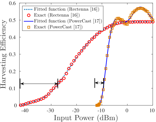
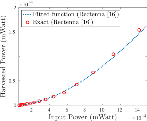
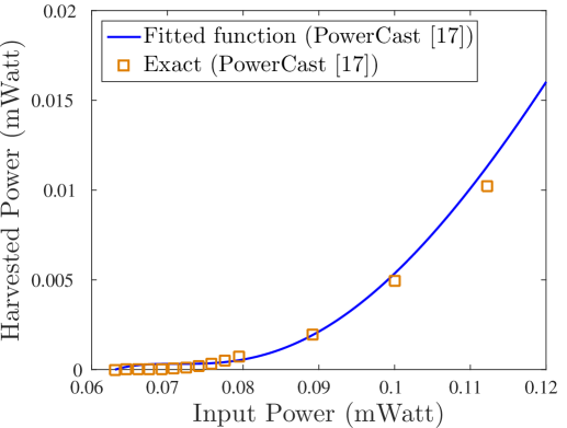
Figure 3: Left: The efficiency of RF harvesting circuit as a function of input power in dBm for (a) the rectenna proposed in [16], depicted with circles and (b) the PowerCast module [17] (at $868$ Mhz), depicted with squares. Center (Right): Harvested power vs. input power in mWatt for input power values depicted with arrows in the left figure for the rectenna in [16] (module in [17]).

The proposed ground-truth model for the harvested power at the output of the RF harvesting circuit is given by:

$$\boldsymbol{P}_{\rm har}^{(n)}\equiv\boldsymbol{P}_{\rm har}^{(n)}\!\left(\boldsymbol{P}_{\rm R}^{(n)}\right)=\mathsf{p}\!\left(\boldsymbol{P}_{\rm R}^{(n)}\right),$$ (6)

where

$$\mathsf{p}(x)\triangleq\begin{cases}0,&x\in[0,\mathtt{P}_{\rm in}^{\rm sen}],\\ \mathsf{e}\!\left(x\right)\cdot x,&x\in[\mathtt{P}_{\rm in}^{\rm sen},\mathtt{P}_{\rm in}^{\rm sat}],\\ \mathsf{e}\!\left(\mathtt{P}_{\rm in}^{\rm sat}\right)\cdot\mathtt{P}_{\rm in}^{\rm sat}&x\in[\mathtt{P}_{\rm in}^{\rm sat},\infty),\end{cases}$$ (7)

where $x$ and $\mathsf{p}(x)$ take values in mWatt. Function $\mathsf{e}\!\left(\cdot\right)$ is the harvesting efficiency as a function of input power, defined over the interval $\mathcal{P}_{\rm in}\triangleq[\mathtt{P}_{\rm in}^{\rm sen},\mathtt{P}_{\rm in}^{\rm sat}].$ $\mathtt{P}_{\rm in}^{\rm sen}$ stands for harvester’s sensitivity; for any input power value smaller than sensitivity, the harvested power is zero, i.e., $\mathsf{p}(x)=0$ for $x\leq\mathtt{P}_{\rm in}^{\rm sen}$. $\mathtt{P}_{\rm in}^{\rm sat}$ denotes the saturation power threshold of the harvester, after which the harvested power is constant.

Harvested power function $\mathsf{p}:\mathds{R}_{+}\longrightarrow\mathds{R}_{+}$ is assumed:

1. non-decreasing, i.e., $x<y\implies\mathsf{p}(x)\leq\mathsf{p}(y)$, and

2. continuous, i.e., $x\longrightarrow x_{0}\implies\mathsf{p}(x)\longrightarrow\mathsf{p}(x_{0})$.

Note that the assumptions above, even though mild, are in full accordance with the harvested power curves reported in the RF energy harvesting circuits’ prior art, e.g., [14, 15, 16, 17].

Determining an explicit formula for $\mathsf{p}(\cdot)$ in (7), for a given rectifier circuit, is crucial task and requires first to specify the harvesting efficiency function $\mathsf{e}\!\left(\cdot\right)$ over the input power interval $\mathcal{P}_{\rm in}$. Inline with the prior art [18, 23, 19, 20, 21, 22], for a given rectifier circuit, some measured harvesting efficiency data points are assumed available, corresponding to some input power values (between sensitivity and saturation). Assuming specific parametrization for $\mathsf{e}\!\left(\cdot\right)$ (e.g., polynomial, sigmoid functions), the measured harvesting efficiency data can be harnessed to designate the best shape for function $\mathsf{e}\!\left(\cdot\right)$ through parameter fitting.

In this work, the ground-truth harvesting efficiency function is modeled as a high-order polynomial in the dBm scale:

$$\mathsf{\mathsf{e}}(x)=w_{0}+\sum_{i=1}^{W}w_{i}(10\,\mathsf{log}_{10}(x))^{i},~{}x\in\mathcal{P}_{\rm in}.$$ (8)

Function in (8) is parametrized by $W+1$ real numbers – the coefficients of the polynomial – where $W$ is the degree of the polynomial. The best values for the coefficients $\{w_{i}\}_{i=0}^{W}$ can be found from the rectenna’s measured harvesting efficiency data, exploiting standard convex optimization fitting techniques from [38, Chapter 6]. The optimized fitted function $\mathsf{\mathsf{e}}(x)$ is non-negative and continuous over $\mathcal{P}_{\rm in}$ and obtains the value zero for $x=\mathtt{P}_{\rm in}^{\rm sen}$. The main benefit of the proposed harvesting efficiency parametrization in (8) is the utilization of dBm scale, that offers higher granularity over the very small input power values. It is emphasized that Eq. (7) will be only used for evaluation of the simplified piecewise linear approximation (proposed in the next section), based on datapoint pairs of harvested power and corresponding input power.

Two rectenna models from the RF harvesting circuit design prior art [16] and [17] are evaluated. The first one is an ultra sensitive rectenna from the microwave theory prior art, while the latter is the PowerCast module. The range of the input power values for the rectenna models [16] and [17] were $\mathcal{P}_{\rm in}=[10^{-4.25},10^{1.6}]$ mWatt and $\mathcal{P}_{\rm in}=[10^{-1.2},10]$ mWatt, respectively. The number of the provided measured data for the rectenna in [16] (PowerCast module [17]) were $118$ and ($53$) points. Fig. 3-Left illustrates the harvesting efficiency as a function of input power in dBm of the two studied rectenna models. Fig. 3-Center (Right) illustrates the harvested power as a function of the input power in mWatt, for the rectenna in [16] (harvester in [17]) and the input power range marked with arrows in Fig. 3-Left; it becomes clear that the harvested power is a nonlinear function of the input power. For the rectenna models in [16] and [17], the degrees of the fitted polynomials for the function $\mathsf{\mathsf{e}}(x)$ are $W=10$ and $W=12$, respectively (depicted in Fig. 3 with dotted and solid curves, respectively).

III-B Impact of Harvester’s Sensitivity in RF Energy Harvesting

The harvester’s sensitivity is a very important parameter playing vital role on the performance of the rectenna. The sensitivity is the power threshold beyond which the rectifier is able to harvest RF energy and depends on diode’s turn-on (or threshold) voltage $\mathtt{V}_{\rm T}$, i.e., the voltage above which the diode is said to be forward-biased [14]. As the turn-on threshold voltage is decreased, the energy conversion efficiency at a given power increases, i.e., the rectifier becomes more sensitive.

Unfortunately, prior art neglects the impact of harvester’s sensitivity. To this end, we define an important RF harvesting metric, given by

$$\mathbb{P}(\boldsymbol{P}_{\rm R}\leq\mathtt{P}_{\rm in}^{\rm sen}),$$ (9)

which is the probability that the input power (depending on the wireless channel) is below the harvester’s sensitivity (depending on the harvester). Note that the probability event of (9) is the fraction of time the rectenna cannot harvest RF energy due to inadequate incident input RF power.

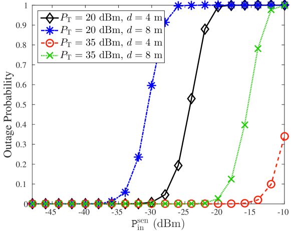
Figure 4: Probability of outage event as a function of harvester’s sensitivity.

Fig. 4 examines the probability of outage in Eq. (9) as a function of harvester’s sensitivity, $\mathtt{P}_{\rm in}^{\rm sen}$. The path-loss model of Eq. (5) is employed with $\nu=2.1$ and Nakagami parameter $\mathtt{m}=5$. It can be clearly deduced that the smaller the harvester’s sensitivity is, the larger the outage probability in (9) becomes. Thus, for the less sensitive PowerCast module [17], the probability of outage due to limited input power is almost $1$ for transmission power $P_{\rm T}=20$ dBm and transmitter-receiver distance $d$ more than $4$ meters, while for $P_{\rm T}=35$ dBm and $d=4$ meters the outage event becomes $10\%$. For the sensitive rectenna in [16] the outage event becomes almost $0$ for all studied scenarios for the parameters $P_{\rm T}$ and $d$. We conclude that the less sensitive the rectenna is, the major the impact of harvester’s sensitivity becomes on the accuracy of the studied RF harvesting model, especially in the low-input-power regime.

III-C Prior Art (Linear) RF Energy Harvesting Models

Three baseline models are considered for comparison:

III-C1 Linear (L) Energy Harvesting Model

The first baseline model is the linear (L) model adopted by a gamut of information and wireless energy transfer prior art; for that model, the harvested power (as function of $\boldsymbol{P}_{\rm R}^{(n)}$) is expressed as follows:

$${\mathsf{p}}_{\rm L}\!\left(x\right)=\eta_{\rm L}\cdot x,~{}x\in\mathds{R}_{+},$$ (10)

with constant $\eta_{\rm L}\in[0,1)$. The functional form of the harvested power in (10) is depicted in Fig. 1 with solid curve. This model ignores the following: (i) the dependence of RF harvesting efficiency on input power, (ii) the harvester cannot operate below the sensitivity threshold, and (iii) the harvested power saturates when the input power level is above a power threshold.

III-C2 Constant-Linear (CL) Energy Harvesting Model

The harvested power is expressed as follows:

$${\mathsf{p}}_{\rm CL}\!\left(x\right)\triangleq\begin{cases}0,&x\in[0,\mathtt{P}_{\rm in}^{\rm sen}],\\ \eta_{\rm CL}\cdot(x-\mathtt{P}_{\rm in}^{\rm sen}),&x\in[\mathtt{P}_{\rm in}^{\rm sen},\infty),\end{cases}$$ (11)

with constant $\eta_{\rm CL}\in[0,1)$. The CL harvested power curve is depicted with dash-dotted line in Fig. 1. This model takes into account the fact that the RF harvester is not able to operate below sensitivity threshold $\mathtt{P}_{\rm in}^{\rm sen}$. On the contrary, the CL model ignores that RF harvesting efficiency is a non-constant function of input power and that the harvested power saturates when the input power is above $\mathtt{P}_{\rm in}^{\rm sat}$.

III-C3 Constant-Linear-Constant (CLC) Energy Harvesting Model

The harvested power is expressed as a function of input power $\boldsymbol{P}_{\rm R}^{(n)}$, through the following expression:

$${\mathsf{p}}_{\rm CLC}\!\left(x\right)\triangleq\begin{cases}0,&x\in[0,\mathtt{P}_{\rm in}^{\rm sen}],\\ \eta_{\rm CLC}\cdot(x-\mathtt{P}_{\rm in}^{\rm sen}),&x\in[\mathtt{P}_{\rm in}^{\rm sen},\mathtt{P}_{\rm in}^{\rm sat}],\\ \eta_{\rm CLC}\cdot(\mathtt{P}_{\rm in}^{\rm sat}-\mathtt{P}_{\rm in}^{\rm sen}),&x\in[\mathtt{P}_{\rm in}^{\rm sat},\infty),\end{cases}$$ (12)

where constant $\eta_{\rm CLC}\in[0,1)$. The CLC model is depicted in Fig. 1 with a dotted curve. This last model ignores the dependence of harvesting efficiency on input power. In our simulation scenarios, parameters $\eta_{\rm L}$, $\eta_{\rm CL}$, and $\eta_{\rm CLC}$ have been chosen empirically to minimize their performance mismatch compared to the real RF harvesting model in Eq. (6).

IV Statistics of Harvested Power

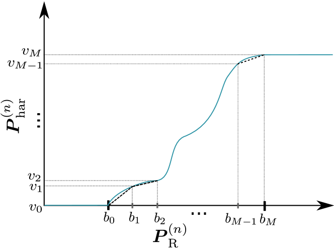
Figure 5: A graphical illustration of the proposed piecewise linear approximation for an RF energy harvesting model, adhering to the mild assumptions of Section III-A.

Consider the harvesting model in Eq. (6) where the function $\mathsf{p}(\cdot)$ satisfies the assumptions in Section III-A. The proposed methodology uses a piecewise linear approximation of $\mathsf{p}(\cdot)$ over interval $\mathcal{P}_{\rm in}$ using $M+1$ points.

Since the harvested power $\boldsymbol{P}_{\rm har}^{(n)}$ in Eq. (6) changes over the range of input power values $\mathcal{P}_{\rm in}$, a set of support points $\{b_{m}\}_{m=0}^{M}$ is defined, with $b_{0}=\mathtt{P}_{\rm in}^{\rm sen}$, $b_{m-1}<b_{m}$, for $m\in[M]$, and $b_{M}=\mathtt{P}_{\rm in}^{\rm sat}$. The corresponding set of image points $\{v_{m}\}_{m=0}^{M}\triangleq\{\mathsf{p}(b_{m})\}_{m=0}^{M}$ satisfy $v_{m-1}=\mathsf{p}(b_{m-1})\leq\mathsf{p}(b_{m})=v_{m}$, $m=1,2,\ldots,M$, with $v_{0}=0$ and $v_{M}=\mathsf{p}(\mathtt{P}_{\rm in}^{\rm sat})$. Without loss of generality, $0=v_{0}<v_{1}<v_{2}<\ldots<v_{M-1}<v_{M}=\mathsf{p}(\mathtt{P}_{\rm in}^{\rm sat})$ is assumed. The methodology is graphically illustrated in Fig. 5.

Given the $M+1$ points $\{b_{m}\}_{m=0}^{M}$ and $\{v_{m}\}_{m=0}^{M}$, slopes $l_{m}\triangleq\frac{v_{m}-v_{m-1}}{b_{m}-b_{m-1}}$, $m\in[M]$ are defined. The utilized methodology approximates $\boldsymbol{P}_{\rm har}^{(n)}$ in Eq. (6) through the following piecewise linear function:

$$\widetilde{\boldsymbol{P}}_{\rm har}^{(n)}\equiv\widetilde{\boldsymbol{P}}_{\rm har}^{(n)}\!\left(\boldsymbol{P}_{\rm R}^{(n)}\right)=\widetilde{\mathsf{p}}\!\left(\boldsymbol{P}_{\rm R}^{(n)}\right)$$ (13)

with

$$\widetilde{\mathsf{p}}(x)\triangleq\begin{cases}0&x\in[0,b_{0}],\\ l_{m}(x-b_{m-1})+v_{m-1},&x\in(b_{m-1},b_{m}],m\in[M],\\ v_{M},&x\in[b_{M},\infty).\end{cases}$$ (14)

The computational complexity to evaluate the function in (14) is $\mathcal{O}(M)$. On the other hand, $\mathcal{O}(1)$ computational cost is required to evaluate the baseline models in Eqs. (10)–(12), the proposed harvested power function in Eq. (7), as well as the harvested power functions from the nonlinear RF harvesting prior art [18, 23, 19, 20, 21, 22]. However, the focus in this work is to assess important RF harvesting performance evaluation metrics in nonlinear RF harvesting, and thus, the computational cost is not a critical issue. One important benefit of the piecewise linear approximation in (13) based on measured input-output datapoints, is its flexibility to interpolate directly the harvested power values, without having the exact functional form of $\mathsf{p}(\cdot)$. Thus, one can directly assess important RF harvesting evaluation metrics without assuming a specific functional form for the harvested power function.

IV-A Statistics of $\widetilde{\boldsymbol{P}}_{\rm har}^{(n)}$ and Approximation Error

This section offers the PDF and CDF of $\widetilde{\boldsymbol{P}}_{\rm har}^{(n)}$. First, the following is defined:

$$\xi_{m}\triangleq\mathsf{F}_{\boldsymbol{P}_{\rm R}^{(n)}}(b_{m}),~{}m=0,1,\ldots,M,$$ (15)

where $\mathsf{F}_{\boldsymbol{P}_{\rm R}^{(n)}}(\cdot)$ is the CDF of $\boldsymbol{P}_{\rm R}^{(n)}$. From Eq. (13) it can be remarked that $\widetilde{\boldsymbol{P}}_{\rm har}^{(n)}=0$ with probability

$$\mathbb{P}\!\left(\boldsymbol{P}_{\rm R}^{(n)}\leq b_{0}\right)=\int_{0}^{b_{0}}\mathsf{f}_{\boldsymbol{P}_{\rm R}^{(n)}}(x)\mathsf{d}x=\mathsf{F}_{\boldsymbol{P}_{\rm R}^{(n)}}(b_{0})=\xi_{0}$$

$$\implies \mathsf{f}_{\widetilde{\boldsymbol{P}}_{\rm har}^{(n)}}(x)=\xi_{0}\,\sDelta(x),~{}x=0.$$ (16)

For any $m\in[M-1]$, when $\boldsymbol{P}_{\rm R}^{(n)}\in(b_{m-1},b_{m}]$, $\widetilde{\boldsymbol{P}}_{\rm har}^{(n)}\in(v_{m-1},v_{m}]$ holds. Thus, using the formula for linear transformations in [39] the following is obtained for any $m\in[M-1]$:

$$\mathsf{f}_{\widetilde{\boldsymbol{P}}_{\rm har}^{(n)}}(x)=\frac{1}{l_{m}}\,\mathsf{f}_{\boldsymbol{P}_{\rm R}^{(n)}}\!\!\left(\frac{x-v_{m-1}+l_{m}b_{m-1}}{l_{m}}\right),$$ (17)

for $x\in(v_{m-1},v_{m}]$. Note that the last interval $\boldsymbol{P}_{\rm R}^{(n)}\in(b_{M-1},b_{M}]$ requires special attention due to the fact that the inverse of function $\widetilde{\mathsf{p}}(\cdot)$ does not exist at point $v_{M}$. Restricting $\boldsymbol{P}_{\rm R}^{(n)}\in(b_{M-1},b_{M})$, the following holds:

$$\mathsf{f}_{\widetilde{\boldsymbol{P}}_{\rm har}^{(n)}}(x)=\frac{1}{l_{M}}\,\mathsf{f}_{\boldsymbol{P}_{\rm R}^{(n)}}\!\!\left(\frac{x-v_{M-1}+l_{M}b_{M-1}}{l_{M}}\right),$$ (18)

for $x\in(v_{M-1},v_{M})$. Finally, in view of (13), $\widetilde{\boldsymbol{P}}_{\rm har}^{(n)}=v_{M}$ with probability given by:

$$\mathbb{P}\!\left(\boldsymbol{P}_{\rm R}^{(n)}\geq b_{M}\right)=1-\lim_{x\rightarrow b_{M}}\mathsf{F}_{\boldsymbol{P}_{\rm R}^{(n)}}(x)\overset{(a)}{=}1-\xi_{M}$$

$$\implies \mathsf{f}_{\widetilde{\boldsymbol{P}}_{\rm har}^{(n)}}(x)=(1-\xi_{M})\,\sDelta(x-v_{M}),~{}x=v_{M},$$ (19)

where $(a)$ stems from the continuity of $\mathsf{F}_{\boldsymbol{P}_{\rm R}^{(n)}}(\cdot)$ as an integral function of a continuous PDF [40], as well as the definition of $\xi_{M}$ in (15). Thus, the following proposition summarizes the results related to the probabilistic description of $\widetilde{\boldsymbol{P}}_{\rm har}^{(n)}$.

Proposition 1.

For a given distribution of the fading power $\boldsymbol{\gamma}^{(n)}$, supported over $\mathds{R}_{+}$, in view of Eq. (2), the corresponding distribution of the input power, $\boldsymbol{P}_{\rm R}^{(n)}$, is $\mathsf{f}_{\boldsymbol{P}_{\rm R}^{(n)}}(x)=\frac{1}{\mathsf{P}(d)}\mathsf{f}_{\boldsymbol{\gamma}^{(n)}}\!\!\left(\frac{x}{\mathsf{P}(d)}\right)$. Hence, the proposed approximation in Eq. (13) has PDF:

$$\mathsf{f}_{\widetilde{\boldsymbol{P}}_{\rm har}^{(n)}}(x)$$

$$= ~{}\begin{cases}\xi_{0}\,\sDelta(x),&x=v_{0}=0,\\ \frac{1}{l_{m}}\,\mathsf{f}_{\boldsymbol{P}_{\rm R}^{(n)}}\!\!\left(\frac{x-v_{m-1}+l_{m}b_{m-1}}{l_{m}}\right),&x\in(v_{m-1},v_{m}]\backslash\{v_{M}\},m\in[M],\\ (1-\xi_{M})\,\sDelta(x-v_{M}),&x=v_{M},\\ 0,&x\in\mathds{R}\backslash[0,v_{M}],\end{cases}$$ (20)

where $m\in[M]$. The corresponding CDF of $\widetilde{\boldsymbol{P}}_{\rm har}^{(n)}$ is given by:

$$\mathsf{F}_{\widetilde{\boldsymbol{P}}_{\rm har}^{(n)}}(x)$$

$$= ~{}\begin{cases}0&x<0,\\ \mathsf{F}_{\boldsymbol{P}_{\rm R}^{(n)}}\!\!\left(\frac{x-v_{m-1}+l_{m}b_{m-1}}{l_{m}}\right),&x\in[v_{m-1},v_{m}]\backslash\{v_{M}\},m\in[M],\\ 1,&x\geq v_{M}.\end{cases}$$ (21)

Proof.

The proof of Eq. (20) is immediate from Eqs. (16)–(19). The proof of Eq. (21) is given in Appendix A. ∎

It is shown immediately below that the proposed approximation in Eq. (14) offers approximation error that decays quadratically with the number of utilized points, even for a uniform choice of points $\{b_{m}\}$, i.e., $b_{m}=b_{m-1}+\delta_{M}$, $m\in[M]$, with $\delta_{M}\triangleq\frac{\mathtt{P}_{\rm in}^{\rm sat}-\mathtt{P}_{\rm in}^{\rm sen}}{M}$.

Proposition 2 (Approximation Error with Uniform Point Selection).

Suppose that we choose $b_{m}=b_{m-1}+\delta_{M}$, $m\in[M]$, with $\delta_{M}$ defined as above. If the function $\mathsf{p}(\cdot)$ is in addition continuously differentiable, then $\widetilde{\mathsf{p}}(\cdot)$ in (14), restricted over $\mathcal{P}_{\rm in}$, approximates $\mathsf{p}(\cdot)$, over $\mathcal{P}_{\rm in}$, with an absolute error that is bounded as follows:

$$\int_{\mathcal{P}_{\rm in}}\left|\mathsf{p}(x)-\widetilde{\mathsf{p}}(x)\right|\mathsf{d}x\leq\frac{\mathtt{C}_{\mathsf{p}}\,(\mathtt{P}_{\rm in}^{\rm sat}-\mathtt{P}_{\rm in}^{\rm sen})^{3}}{8\,M^{2}},$$ (22)

where $\mathtt{C}_{\mathsf{p}}=\max_{x\in\mathcal{P}_{\rm in}}\left|\mathsf{p}^{\prime\prime}(x)\right|$ is a constant independent of $M$.

Proof.

The proof is provided in Appendix B. ∎

Thus, at most $\mathcal{O}\!\left(\sqrt{\frac{1}{\epsilon}}\right)$ number of support points is required to approximate the function $\mathsf{p}(\cdot)$ with accuracy at least $\epsilon$.

V Evaluation

V-A Baseline Comparison: Average Harvested Energy

For baseline comparison, the expected harvested energy is considered. $\boldsymbol{U}_{N}\triangleq\sum_{n=1}^{N}\boldsymbol{P}_{\rm har}^{(n)}$ denotes the accumulated harvested power up to coherence block $N$, which in turn offers the expected harvested energy over $N$ coherence periods:

$$\mathbb{E}\!\left[T_{\rm p}\,\boldsymbol{U}_{N}\right]=T_{\rm p}\,\mathbb{E}\!\left[\sum_{n=1}^{N}\boldsymbol{P}_{\rm har}^{(n)}\right]=N\,T_{\rm p}\,\mathbb{E}\!\left[\boldsymbol{P}_{\rm har}^{(n)}\right],$$ (23)

for some $n\in[N]$. The last equality stems from the fact that $\{\boldsymbol{P}_{\rm har}^{(n)}\}_{n\in[N]}$ are identically distributed, since $\{\boldsymbol{\gamma}^{(n)}\}_{n\in[N]}$ are also identically distributed. Let us denote $\overline{\mathtt{P}}_{\rm L}$, $\overline{\mathtt{P}}_{\rm CL}$, $\overline{\mathtt{P}}_{\rm CLC}$, and $\overline{\widetilde{\mathtt{P}}}$ the expected harvested power over a single coherence block of the following models, respectively: linear in Eq. (10), constant-linear in Eq. (11), constant-linear-constant in Eq. (12), and proposed in Eq. (13).

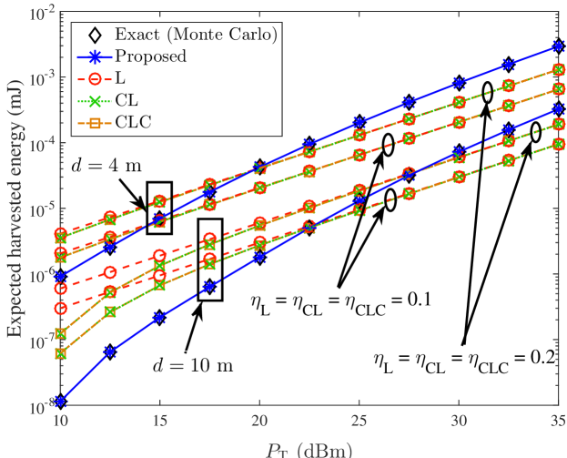
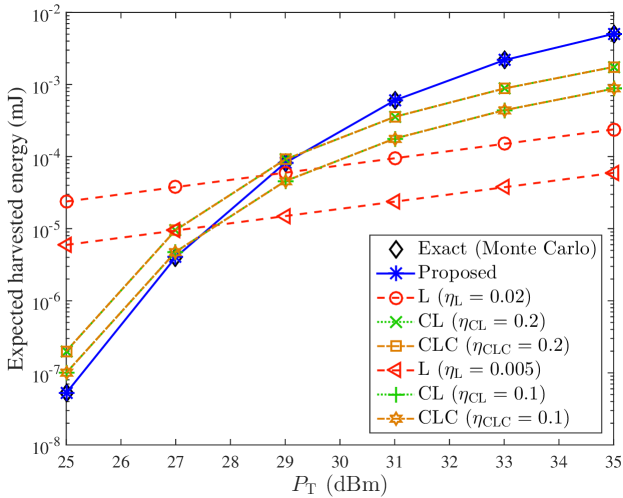
Figure 6: Left (Right): Expected harvested energy per coherence block ($N=1$) vs. transmission power $P_{\rm T}$ for the rectenna proposed in [16] (harvesting module in [17]).

Under Nakagami fading, the average harvested power for the baseline linear models is given by:

$$\overline{\mathtt{P}}_{\rm L} =\mathbb{E}[{\mathsf{p}}_{\rm L}(\boldsymbol{P}_{\rm R})]=\eta_{\rm L}\,\mathsf{P}(d)$$ (24)

$$\overline{\mathtt{P}}_{\rm CL} =\mathbb{E}[{\mathsf{p}}_{\rm CL}(\boldsymbol{P}_{\rm R})]=\int_{0}^{\infty}\!{\mathsf{p}}_{\rm CL}(x)\,\mathsf{f}_{\boldsymbol{P}^{(n)}_{\rm R}}(x)\mathsf{d}x$$

$$=\eta_{\rm CL}\left(\frac{\mathsf{P}(d)\,\sGamma\!\left(\mathtt{m}+1,\frac{\mathtt{m}}{\mathsf{P}(d)}\mathtt{P}_{\rm in}^{\rm sen}\right)}{\Gamma(\mathtt{m}+1)}-\frac{\mathtt{P}_{\rm in}^{\rm sen}\,\sGamma\!\left(\mathtt{m},\frac{\mathtt{m}}{\mathsf{P}(d)}\mathtt{P}_{\rm in}^{\rm sen}\right)}{\Gamma(\mathtt{m})}\right)$$ (25)

$$\overline{\mathtt{P}}_{\rm CLC} =\mathbb{E}[{\mathsf{p}}_{\rm CLC}(\boldsymbol{P}_{\rm R})]=\int_{0}^{\infty}{\mathsf{p}}_{\rm CLC}(x)\,\mathsf{f}_{\boldsymbol{P}^{(n)}_{\rm R}}(x)\mathsf{d}x$$

$$=\left(\frac{\mathsf{P}(d)\left(\sGamma\!\left(\mathtt{m}+1,\frac{\mathtt{m}}{\mathsf{P}(d)}\mathtt{P}_{\rm in}^{\rm sen}\right)-\sGamma\!\left(\mathtt{m}+1,\frac{\mathtt{m}}{\mathsf{P}(d)}\mathtt{P}_{\rm in}^{\rm sat}\right)\right)}{\Gamma(\mathtt{m}+1)}\right.$$

$$+\left.\!\frac{\mathtt{P}_{\rm in}^{\rm sat}\,\sGamma\!\left(\mathtt{m},\frac{\mathtt{m}}{\mathsf{P}(d)}\mathtt{P}_{\rm in}^{\rm sat}\right)}{\Gamma(\mathtt{m})}-\frac{\mathtt{P}_{\rm in}^{\rm sen}\,\sGamma\!\left(\mathtt{m},\frac{\mathtt{m}}{\mathsf{P}(d)}\mathtt{P}_{\rm in}^{\rm sen}\right)}{\Gamma(\mathtt{m})}\right)\eta_{\rm CLC},$$ (26)

where the expressions above rely on $\Gamma(\mathtt{m}+1)=\mathtt{m}\cdot\Gamma(\mathtt{m})$, as well as on the following formula ($i\in\mathds{N}\cup\{0\}$) [41, Eq. (3.381.9)]:

$$\int_{a}^{b}\!\!x^{i}\,\mathsf{f}_{\boldsymbol{P}^{(n)}_{\rm R}}(x)\mathsf{d}x=\left(\frac{\mathsf{P}(d)}{\mathtt{m}}\right)^{i}\,\frac{\sGamma\!\left(\mathtt{m}+i,\frac{\mathtt{m}}{\mathsf{P}(d)}a\right)-\sGamma\!\left(\mathtt{m}+i,\frac{\mathtt{m}}{\mathsf{P}(d)}b\right)}{\Gamma(\mathtt{m})}.$$ (27)

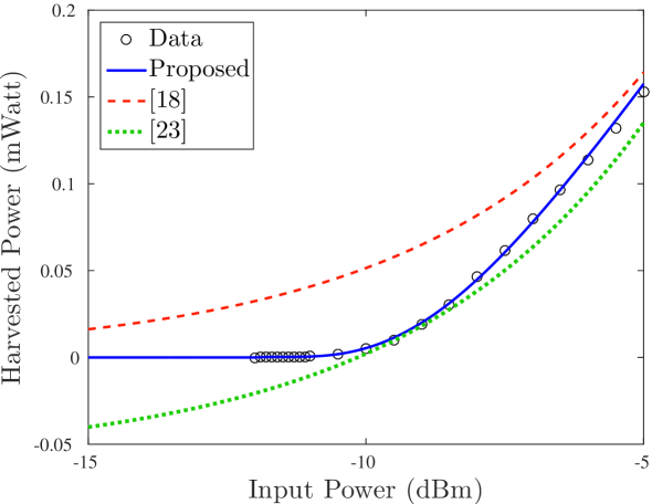
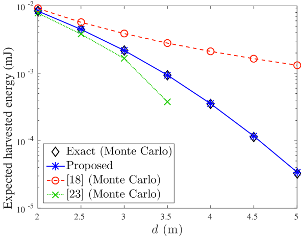
Figure 7: Left: Harvested power vs. input power for the proposed and the other nonlinear RF harvesting models from the prior art using the harvesting module in [17]. Right: Expected harvested energy per coherence block ($N=1$) vs. distance $d$.

For the proposed piecewise linear approximation, the expected harvested power over a single coherence period is given by:

$$\overline{\widetilde{\mathtt{P}}} =\mathbb{E}[\widetilde{\mathsf{p}}(\boldsymbol{P}_{\rm R})]$$

$$=\sum_{j=1}^{M}\left(\frac{l_{j}\,\mathsf{P}(d)\left(\sGamma\!\left(\mathtt{m}+1,\frac{\mathtt{m}\,b_{j-1}}{\mathsf{P}(d)}\right)-\sGamma\!\left(\mathtt{m}+1,\frac{\mathtt{m}\,b_{j}}{\mathsf{P}(d)}\right)\right)}{\Gamma(\mathtt{m}+1)}\right.$$

$$\left.+\frac{(v_{j-1}-l_{j}b_{j-1})\left(\sGamma\!\left(\mathtt{m},\frac{\mathtt{m}\,b_{j-1}}{\mathsf{P}(d)}\right)-\sGamma\!\left(\mathtt{m},\frac{\mathtt{m}\,b_{j}}{\mathsf{P}(d)}\right)\right)}{\Gamma(\mathtt{m})}\right)$$

$$~{}+\frac{v_{M}\,\sGamma\!\left(\mathtt{m},\frac{\mathtt{m}}{\mathsf{P}(d)}\mathtt{P}_{\rm in}^{\rm sat}\right)}{\Gamma(\mathtt{m})},$$ (28)

where Eq. (27) is exploited to obtain the final simplified expression.

V-A1 Numerical Results

The expected harvested energy in Eq. (23) is found for the actual energy harvesting model in Eq. (6) (obtained through Monte Carlo experiments), for the three linear baseline models, and the proposed piecewise linear energy harvesting model.

Fig. 6 examines the impact of transmit power $P_{\rm T}$ on the average harvested energy over $N=1$ coherence period using $T_{\rm p}=50$ msec. In Fig. 6-Left, $\nu=2.1$ and $\mathtt{m}=5$ are set, for the rectenna in [16]. It can be observed that the expected harvested energy performance of the proposed approximation in (13) with $M+1=586$ points is the same with the performance of the actual harvesting model for all studied distance scenarios of $d=4$ and $d=10$ meters. Thus, the approximation with the specific number $M$ of points is accurate. The slope of the expected harvested energy for the baseline (linear) schemes is different compared to the exact model, demonstrating their mismatch compared to the reality.

In Fig. 6-Right, using the same small- and large-scale fading parameters as above, $M+1=221$ approximation points, and distance $d=3$ m, it is shown that the linear model is highly inaccurate for the second harvesting circuit module; thus, the widely adopted linear model cannot capture realistic efficiency models. The performance of the other two baseline linear models is closer to the actual harvesting model. However, the slopes are different and a non-negligible mismatch still exists.

Next, in Fig. 7-Left, we depict the measured harvested power data from [17] over the input power range $[-15,-5]$ dBm, as well as the fitted harvested power functions obtained from: (a) the proposed model in (7) and (b) the two nonlinear models proposed in [18, 23]. For the nonlinear models of prior art, the normalized sigmoid function [18, Eqs. (4) and (5)] and the second-order polynomial in milliWatt scale [23, Eq. (5)] are utilized. The optimal parameters of the fitted functions are obtained using the Matlab’s fitting toolbox. It can remarked that the proposed ground-truth harvested power model in Eq. (6) fits perfectly to the measured data. The curve obtained using the sigmoid function in [18] tends to overestimate the measured harvested power for the small values of input power, while the second-order polynomial in [23] underestimates the harvested power for the input power near sensitivity, offering negative harvested power values for input power less than $-10$ dBm.

In Fig. 7-Right we depict the expected harvested energy as a function of distance using $P_{\rm T}=2$ Watt comparing the above harvested power models. The path-loss model of Eq. (5) is employed with $\nu=2.1$ and $\mathtt{m}=5$. The proposed piecewise linear approximation in Eq. (13) interpolates directly the measured $M+1=53$ data points without using any fitting. The harvested power model in [18] overestimates the expected harvested energy for large distances, deviating quite much from the reality. This stems directly from the fact that the sensitivity effects of the harvester are ignored in that model. On the other hand, the performance of the model in [23] tends to underestimate the expected harvested energy, attaining negative values for $d>3.5$. Compared to [18], the model in [23] offers more accurate expected harvested energy performance for $d\leq 3.5$. The proposed piecewise linear approximation, interpolating directly the measured harvested power data, achieves the same performance with the exact model.

V-B Time-Switching RF Energy Harvesting Scenario: Expected Charging Time

Figure 8: Time-switching operation. Necessary energy is harvested before the communication, in duty-cycled, non-continuous applications (e.g., wireless sensors).

Another important metric is the expected time for the RF harvesting circuit to charge its storage unit at the minimum required level, before operation. This is graphically illustrated in Fig. 8, showing the time-switching RF energy harvesting and communication protocols, where the terminal (e.g., a wireless sensor) first scavenges the necessary energy for transmission and then communicates (e.g., work in [16]). This is typical in many RF harvesting protocols, since the available power density in $\mu$Watt/cm² is limited and cannot sustain the power requirements of the overall apparatus; thus, a duty-cycled, non-continuous operation is necessary, as depicted in Fig. 8. The time needed to harvest the necessary energy before operation should be accurately quantified.

An energy harvesting outage event after $N$ coherence periods will occur if the harvested energy after $N$ coherence periods is below a threshold. The latter is determined by the capacity of the energy storage unit (e.g., a capacitor $\mathtt{C}$) and the operating voltage $\mathtt{V}$ of the harvesting circuit. Thus, the outage event is given by:

$$\mathscr{O}_{N}\triangleq ~{}\left\{T_{\rm p}\,\sum_{n=1}^{N}\boldsymbol{P}_{\rm har}^{(n)}\leq\frac{1}{2}\,\mathtt{C}\,\mathtt{V}^{2}\right\}=\left\{\sum_{n=1}^{N}\!\boldsymbol{P}_{\rm har}^{(n)}\leq\theta_{\rm harv}^{\rm th}\right\},$$ (29)

where the power threshold is determined by the minimum required stored energy for operation $\frac{1}{2}\,\mathtt{C}\,\mathtt{V}^{2}$, as well as the transmission duration $T_{\rm p}$, i.e., $\theta_{\rm harv}^{\rm th}\triangleq\frac{\mathtt{C}\,\mathtt{V}^{2}}{2\,T_{\rm p}}$. Note that the above event depends on the fading coefficients $\{\boldsymbol{\gamma}^{(n)}\}_{n\in[N]}$.

The RV $\boldsymbol{N}^{\star}$ is defined as the first coherence time index when the accumulated harvested power is above the power threshold $\theta_{\rm harv}^{\rm th}$, given that there exist $\boldsymbol{N}^{\star}-1$ consecutive outage events; thus, the probability mass function (PMF) of RV $\boldsymbol{N}^{\star}$ can be derived as:

$$\mathbb{P}(\boldsymbol{N}^{\star}=N)$$

$$\triangleq \mathbb{P}\left(\mathscr{O}_{N-1}\cap\left\{\boldsymbol{P}_{\rm har}^{(N)}>\theta_{\rm harv}^{\rm th}-\sum_{n=1}^{N-1}\!\boldsymbol{P}_{\rm har}^{(n)}\right\}\right)$$

$$= \mathbb{P}\left(\sum_{n=1}^{N-1}\!\boldsymbol{P}_{\rm har}^{(n)}\leq\theta_{\rm harv}^{\rm th}\cap\boldsymbol{P}_{\rm har}^{(N)}>\theta_{\rm harv}^{\rm th}-\sum_{n=1}^{N-1}\!\boldsymbol{P}_{\rm har}^{(n)}\right)$$

$$\overset{(a)}{=} \mathbb{P}\!\left(\boldsymbol{U}_{N-1}\leq\theta_{\rm harv}^{\rm th}\cap\boldsymbol{U}_{N-1}>\theta_{\rm harv}^{\rm th}-\boldsymbol{P}_{\rm har}^{(N)}\right)$$

$$\overset{(b)}{=} \!\!\int_{x\in\mathbf{dom}\mathsf{f}_{\boldsymbol{P}_{\rm har}}}\!\!\!\!\!\!\!\!\!\!\!\mathbb{P}\!\left(\boldsymbol{U}_{N-1}\leq\theta_{\rm harv}^{\rm th}\cap\boldsymbol{U}_{N-1}>\theta_{\rm harv}^{\rm th}-x\right)\,\mathsf{f}_{\boldsymbol{P}_{\rm har}^{(N)}}(x)\mathsf{d}x$$

$$\overset{(c)}{=} \mathsf{F}_{\boldsymbol{U}_{N-1}}\!(\theta_{\rm harv}^{\rm th})-\!\int_{x\in\mathbf{dom}\mathsf{f}_{\boldsymbol{P}_{\rm har}}}\!\!\!\!\mathsf{F}_{\boldsymbol{U}_{N-1}}\!(\theta_{\rm harv}^{\rm th}-x)\,\mathsf{f}_{\boldsymbol{P}_{\rm har}^{(N)}}(x)\mathsf{d}x,$$ (30)

where step $(a)$ used the definition of RV $\boldsymbol{U}_{N}$, i.e., $\boldsymbol{U}_{N-1}=\sum_{n=1}^{N-1}\!\boldsymbol{P}_{\rm har}^{(n)}$, step $(b)$ exploited the law of iterated expectation and the fact that $\boldsymbol{U}_{N-1}$ and $\boldsymbol{P}_{\rm har}^{(N)}$ are independent, and step $(c)$ employed the CDF definition. Note that the expression above requires the CDF of $\boldsymbol{U}_{N-1}$, which will be offered subsequently, while PDF of $\boldsymbol{P}_{\rm har}^{(N)}$ can be given with the methodology of Section IV-A.

The expected value of discrete RV $\boldsymbol{N}^{\star}$ can be easily calculated as:

$$\mathbb{E}[\boldsymbol{N}^{\star}]\triangleq\overline{N}^{\star}=\sum_{N=1}^{\infty}N\cdot\mathbb{P}(\boldsymbol{N}^{\star}=N).$$ (31)

The physical meaning of $\overline{{N}}^{\star}$ is the average number of coherence periods, i.e., $\overline{{N}}^{\star}\,T_{\rm c}$ seconds, required for the capacitor charging, before the communication. Such expected charging time is a prerequisite time interval, necessary for scavenging adequate RF energy for any subsequent operation.

A numerical methodology to calculate ${\overline{N}}^{\star}$ is provided for the proposed approximation model in (13). To calculate ${\overline{N}}^{\star}$ for the proposed model, Eq. (30) must be exploited using $\widetilde{\boldsymbol{U}}_{N-1}\triangleq\sum_{n=1}^{N-1}\!\widetilde{\boldsymbol{P}}_{\rm har}^{(n)}$ and $\widetilde{\boldsymbol{P}}_{\rm har}^{(N)}$. However, only the PDF of each individual RV $\widetilde{\boldsymbol{P}}_{\rm har}^{(n)}$, $n\in[N]$, is known. Hence, a methodology to calculate the CDF and the PDF of $\widetilde{\boldsymbol{U}}_{N-1}$ is proposed, exploiting the fact that the latter can be written as a sum of independent RVs. The proposed methodology to evaluate Eq. (30), and thus $\overline{N}^{\star}$, is provided in Appendix C. Applying the methodology presented in Appendix C, the PMF of RV $\boldsymbol{N}^{\star}$ is calculated for the proposed model using Eq. (55) for any threshold $\theta_{\rm harv}^{\rm th}$.

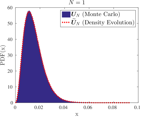
Figure 9: The histogram of actual $\boldsymbol{U}_{N}$ and the corresponding PDF vector $\mathbf{\underline{v}}_{\mathsf{f}}$ for $N=1$, $N=20$, and $N=50$ for the energy harvesting model in [16].

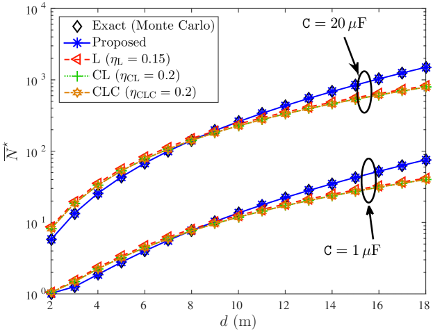
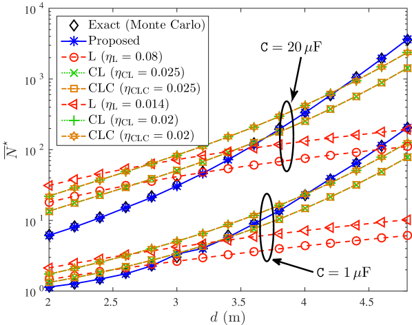
Figure 10: Left (Right): Expected number of coherence periods $\boldsymbol{N}^{\star}$, $\overline{N}^{\star}$, necessary for charging vs. distance for the rectenna proposed in [16] (PowerCast module [17]).

Consider the rectenna model in [16], the path-loss model given in (5) with $\nu=2.1$ and $d=5$ m, transmission power $P_{\rm T}=1.5$ Watt, Nakagami parameter $\mathtt{m}=5$, while the parameters for the power threshold are set to $\mathtt{V}=1.8$ V, $\mathtt{C}=10$ $\mu$F, $T_{\rm p}=50$ msec. Fig. 9 shows the histogram of actual $\boldsymbol{U}_{N}$ and the corresponding estimated PDF of RV $\widetilde{\boldsymbol{U}}_{N}$, for $N=1$, $N=20$, and $N=50$. It can be seen that the red dotted curves corresponding to the estimated PDFs, and the actual PDF (histogram) are perfectly matched.

V-B1 Numerical Results

Fig. 10 depicts the expected $N^{\star}$ for the realistic, proposed, and baseline models as a function of distance for different capacitor values ($\mathtt{C}=1$ $\mu$F and $\mathtt{C}=20$ $\mu$F) for the two harvesting efficiency models in [16] (Left) and [17] (Right) using $\mathtt{V}=1.8$ V and $T_{\rm p}=50$ msec. The path-loss model in Eq. (5) is employed for the evaluation in conjunction with Nakagami fading. In Fig. 10-Left (Right) the utilized wireless channel parameters are $\nu=2.1$, $\mathtt{m}=5$, $P_{\rm T}=1.5$ Watt, while for the density evolution, the following parameters are employed $H=2^{17}$ and $J_{\rm FFT}=2^{18}$ ($J_{\rm FFT}=2^{19}$). The number of data points to approximate the harvested power in Eq. (13) was $M+1=1171$ and $M+1=2201$ data points for the rectennas in [16] and [17], respectively.

For both harvesting efficiency models in [16] and [17] the expected charging time for the proposed approximation and the true, nonlinear harvested power model coincide, corroborating the accuracy of a) the proposed approximation in Eq. (13) and b) the framework in Appendix C.

For the baseline models, the results are obtained through Monte Carlo. It is observed that although the results for baseline models are offered with the best possible values for $\eta_{\rm L}$, $\eta_{\rm CL}$, and $\eta_{\rm CLC}$, the baseline linear harvesting efficiency models fail to offer the same slope with the true, nonlinear energy harvesting model; as a result, the obtained $N^{\star}$ for the linear models may deviate one order of magnitude from the true value, offering consequently deviations from the true duty-cycle and the available resources for wireless communications. It is also noted that the presence of a boost converter at the rectifier output may also magnify the necessary time for charging, further amplifying the charging time differences. The proposed methodology with the nonlinear harvesting model is clearly able to offer accurate estimation of the charging time.

V-C Power-Splitting RF Energy Harvesting Scenario: Passive RFID Tags

Figure 11: The power-splitting operation mode.

Next, a backscatter RFID scenario is considered where the EIH node is a passive RFID tag that splits the input RF power for operation and wireless communication, simultaneously (Fig. 11), as opposed to the time-switching (duty-cycled) operation. The passive RFID tags typically use a simple RF switch (e.g., a transistor) to communicate with an interrogator.

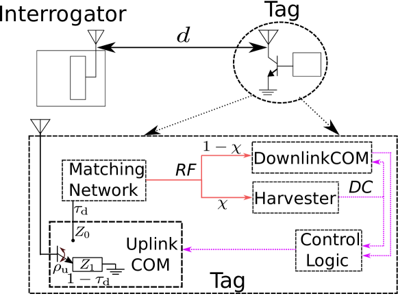
Figure 12: A monostatic backscatter architecture consisting of an interrogator (i.e., an RFID reader) and a passive RFID tag. The interrogator’s antenna acts as the transmitter of illuminating signal, as well as the receiver of reflected, i.e., the backscattered (from tag) information, hence the term monostatic.

A typical operating block diagram of a passive RFID tag is depicted in Fig. 12. Suppose that the tag’s antenna is terminated between two load values $Z_{0}$ and $Z_{1}$. When the antenna is terminated at $Z_{0}$, it is matched to input load and the tag absorbs the power from the incident signal. When the antenna is terminated at load $Z_{1}$, the tag reflects the incoming signal, i.e., it scatters back information (uplink), provided that it has sufficient amount of energy. It is further assumed that the overall round-trip communication among the interrogator and the tag lasts a single coherence time period, thus we focus on a single coherence time block; thereinafter, coherence block index $n$ is removed to simplify the notation.

Parameter $\tau_{\rm d}$ denotes the fraction of time the antenna load is at $Z_{0}$ (absorbing state), while the rest $1-\tau_{\rm d}$ corresponds to fraction of time at load $Z_{1}$ (reflection state). Assume that $\chi$ is the fraction of the input power (when tag’s antenna load is at absorbing state) dedicated for the RF energy harvesting operation; thus, a total of $\zeta_{\rm har}=\chi\,\tau_{\rm d}$ percentage of the input power is dedicated for energy harvesting, with $\zeta_{\rm har}\in(0,1)$. The rest $(1-\chi)\tau_{\rm d}$ input signal power is exploited by the tag downlink communication circuitry. Furthermore, a fraction $\rho_{\rm u}\leq 1-\tau_{\rm d}$ of the impinged power is used for the uplink scatter radio operation. This number depends on the scattering efficiency and the fraction of time the tag’s antenna is terminated at the load $Z_{1}$. It is noted that the scattering efficiency depends on the reflection coefficients, which in turn are input power-independent. With monostatic architecture, the incident input power at tag is $\boldsymbol{P}_{\rm R}=P_{\rm T}\,\mathsf{L}(d)\,\boldsymbol{\gamma}=\mathsf{P}(d)\boldsymbol{\gamma}$. Since, only a fraction $\rho_{\rm u}$ of the input power is backscattered (i.e., $\rho_{\rm u}\,\boldsymbol{P}_{\rm R}$), the received power at the interrogator due to the round trip nature of backscattering operation is

$$\mathsf{g}_{\rm int}(\boldsymbol{P}_{\rm R})\triangleq\rho_{\rm u}\,\boldsymbol{P}_{\rm R}\,\mathsf{L}(d)\,\gamma=\rho_{\rm u}\frac{(\boldsymbol{P}_{\rm R})^{2}}{P_{\rm T}}.$$ (32)

The two following events are needed:

$$\mathscr{A} \triangleq\{\text{The BER at the interrogator is below a threshold $\beta$}\}$$

$$=\left\{2\,\mathsf{Q}\!\left(\frac{\sqrt{\mathsf{g}_{\rm int}(\boldsymbol{P}_{\rm R})}}{\sigma_{\rm u}}\right)\left(1-\mathsf{Q}\!\left(\frac{\sqrt{\mathsf{g}_{\rm int}(\boldsymbol{P}_{\rm R})}}{\sigma_{\rm u}}\right)\right)<\beta\right\}$$ (33)

and

$$\mathscr{B} \triangleq\{\text{\small The harvested power is larger than tags' power consumption $\mathtt{P}_{\rm c}$}\}$$

$$=\left\{\mathsf{p}(\zeta_{\rm har}\,\boldsymbol{P}_{\rm R})>\mathtt{P}_{\rm c}\right\},$$ (34)

where $\mathsf{Q}(x)=\frac{1}{\sqrt{2\pi}}\int_{x}^{\infty}\mathsf{e}^{-\frac{t^{2}}{2}}\mathsf{d}t$ is the Q-function and the expression in the last line of Eq. (33) is the probability of bit error under coherent maximum-likelihood detection with FM$0$ line coding [42], and $\beta\in(0,\frac{1}{2})$ is the BER threshold. Parameter $\sigma_{\rm u}^{2}$ is a properly scaled variance of thermal AWGN noise at the receiving circuit of the interrogator. The expression in (33) can be further simplified with the aid of the following:

Proposition 3.

The function

$$y=\mathsf{R}(x)\triangleq 2\,\mathsf{Q}(x)\,(1-\mathsf{Q}(x)),~{}x\in(0,\infty),$$ (35)

is monotone decreasing and invertible over the positive reals; the inverse function is given by

$$x=\mathsf{R}^{-1}(y)=\mathsf{Q}^{-1}\!\left(\frac{1-\sqrt{1-2\,y}}{2}\right),~{}y\in(0,0.5),$$ (36)

where the function $\mathsf{Q}^{-1}(\cdot)$ denotes the inverse of Q-function (with respect to composition).

Proof.

The proof is given in Appendix D. ∎

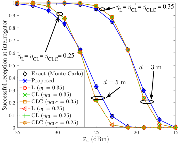
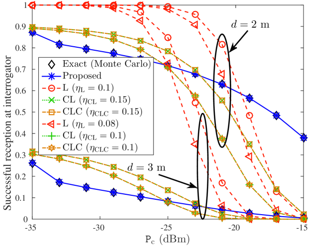
Figure 13: Left (Right): The probability of successful reception at interrogator as a function of tags’ power consumption $\mathtt{P}_{\rm c}$ and tag-interrogator distance, for the rectenna model in [16] (PowerCast module [17]).

The event of the successful interrogator reception is denoted by $\mathscr{S}$; the non-successful reception event at the interrogator, $\mathscr{S}^{\rm C}$, occurs if a) the harvested power is below the tag’s power consumption or (b) given that the harvested power is above the tag’s power consumption $\mathtt{P}_{\rm c}$, the BER at the interrogator is above the threshold $\beta$:

$$\mathbb{P}(\mathscr{S}^{\rm C}) =\mathbb{P}(\mathscr{B}^{\rm C})+\mathbb{P}(\mathscr{A}^{\rm C}|\mathscr{B})\mathbb{P}(\mathscr{B})=1-\mathbb{P}(\mathscr{B})+\mathbb{P}(\mathscr{A}^{\rm C}|\mathscr{B})\mathbb{P}(\mathscr{B})$$

$$=1-\mathbb{P}(\mathscr{B})(1-\mathbb{P}(\mathscr{A}^{\rm C}|\mathscr{B}))=1-\mathbb{P}(\mathscr{B})\mathbb{P}(\mathscr{A}|\mathscr{B})$$

$$=1-\mathbb{P}(\mathscr{A}\cap\mathscr{B})=1-\mathbb{P}(\mathscr{S}).$$ (37)

Thus, in view of Eq. (37), the probability of successful event is expressed as:

$$\mathbb{P}(\mathscr{S})= ~{}\mathbb{P}\left(\mathsf{R}\!\left(\frac{\sqrt{\mathsf{g}_{\rm int}(\boldsymbol{P}_{\rm R})}}{\sigma_{\rm u}}\right)<\beta\cap\mathsf{p}(\zeta_{\rm har}\,\boldsymbol{P}_{\rm R})>\mathtt{P}_{\rm c}\right)$$

$$\overset{(a)}{=} ~{}\mathbb{P}\!\left(\boldsymbol{P}_{\rm R}>\frac{\sqrt{P_{\rm T}}\,\mathsf{R}^{-1}(\beta)\sigma_{\rm u}}{\sqrt{\rho_{\rm u}}}\cap\mathsf{p}(\zeta_{\rm har}\,\boldsymbol{P}_{\rm R})>\mathtt{P}_{\rm c}\right),$$ (38)

where in step $(a)$ we exploited the fact that the function $\mathsf{R}^{-1}$ in (36) is monotone decreasing and then we plugged the definition of function $\mathsf{g}_{\rm int}(\cdot)$.

The corresponding probability expressions can be derived for the baseline linear models and the proposed nonlinear harvesting model. The successful reception event at the interrogator for baseline models is denoted as $\mathscr{S}_{\rm c}$, $\rm c\in\{L,CL,CLC\}$ and for the proposed model as $\widetilde{\mathscr{S}}$. The following proposition summarizes the results:

Proposition 4.

Suppose that $\mathtt{P}_{\rm c}>0$ and consider Nakagami fading. Let us define threshold $\theta_{\mathscr{A}}\triangleq\frac{\sqrt{P_{\rm T}}\,\mathsf{R}^{-1}(\beta)\sigma_{\rm u}}{\sqrt{\rho_{\rm u}}}>0$. For the linear model, the probability of event $\mathscr{S}_{\rm L}$ is given by:

$$\mathbb{P}(\mathscr{S}_{\rm L})=\frac{\sGamma\!\left(\mathtt{m},\frac{\mathtt{m}}{\mathsf{P}(d)}\theta_{\rm max}^{\rm L}\right)}{\Gamma(\mathtt{m})},$$ (39)

where $\theta_{\rm max}^{\rm L}\triangleq\max\{\theta_{\mathscr{A}},\frac{\mathsf{p}_{\rm L}^{-1}(\mathtt{P}_{\rm c})}{\zeta_{\rm har}}\}$.

For the constant-linear model, the probability of event $\mathscr{S}_{\rm CL}$ is given by:

$$\mathbb{P}(\mathscr{S}_{\rm CL})=\frac{\sGamma\!\left(\mathtt{m},\frac{\mathtt{m}}{\mathsf{P}(d)}\theta_{\rm max}^{\rm CL}\right)}{\Gamma(\mathtt{m})},$$ (40)

where $\theta_{\rm max}^{\rm CL}\triangleq\max\{\theta_{\mathscr{A}},\frac{\mathsf{p}_{\rm CL}^{-1}(\mathtt{P}_{\rm c})}{\zeta_{\rm har}}\}$.

For the last baseline model (CLC), the probability of event $\mathscr{S}_{\rm CLC}$ is expressed as follows:

$$\mathbb{P}(\mathscr{S}_{\rm CLC})=\begin{cases}\frac{\sGamma\left(\mathtt{m},\frac{\mathtt{m}}{\mathsf{P}(d)}\theta_{\rm max}^{\rm CLC}\right)}{\Gamma(\mathtt{m})},&0<\mathtt{P}_{\rm c}<\mathsf{p}_{\rm CLC}(\mathtt{P}_{\rm in}^{\rm sat}),\\ 0,&\mathtt{P}_{\rm c}\geq\mathsf{p}_{\rm CLC}(\mathtt{P}_{\rm in}^{\rm sat}),\end{cases}$$ (41)

where $\theta_{\rm max}^{\rm CLC}\triangleq\max\{\theta_{\mathscr{A}},\frac{\mathsf{p}_{\rm CLC}^{-1}(\mathtt{P}_{\rm c})}{\zeta_{\rm har}}\}$.

Finally, for the proposed nonlinear energy harvesting model, the probability of event $\widetilde{\mathscr{S}}$ is given by:

$$\mathbb{P}(\widetilde{\mathscr{S}})=\begin{cases}\frac{\sGamma\!\left(\mathtt{m},\frac{\mathtt{m}}{\mathsf{P}(d)}\widetilde{\theta}_{\rm max}\right)}{\Gamma(\mathtt{m})},&0<\mathtt{P}_{\rm c}<v_{M},\\ 0,&\mathtt{P}_{\rm c}\geq v_{M},\end{cases}$$ (42)

where $\widetilde{\theta}_{\rm max}\triangleq\max\{\theta_{\mathscr{A}},\frac{\widetilde{\mathsf{p}}^{-1}(\mathtt{P}_{\rm c})}{\zeta_{\rm har}}\}$.

Proof.

The proof can be found in Appendix E. ∎

V-C1 Numerical Results

Fig. 13 offers the probability of successful reception at the interrogator, as function of the tag power consumption $\mathtt{P}_{\rm c}$ and the tag-interrogator distance under the path-loss model of Eq. (5). The following parameters are utilized: $\tau_{\rm d}=0.5$, $\chi=0.5$, $\rho_{\rm u}=0.01$, $\beta=10^{-5}$, $\sigma_{\rm u}^{2}=10^{-11}$ mWatt. In Fig. 13-Left (Right) the rectenna model in [16] (harvesting module in [17]) is studied using parameters $\nu=2.1$, $\mathtt{m}=5$, $P_{\rm T}=1.5$ Watt ($P_{\rm T}=3$ Watt), under two distance setups: $d=5$ m and $d=3$ m ($d=3$ m and $d=2$ m), and using $M+1=586$ ($M+1=221$) data points.

From both figures it can be seen that the performance of the proposed approximation in Eq. (13) is the same with the performance of the real model in Eq. (6). On the other hand, the baseline models offer different slopes compared to the nonlinear model and fail to approach its performance; this holds for both harvesting circuits, even though deviations are more obvious for the harvester in [17]; it is also noted that the selected values of $\eta_{\rm L}$, $\eta_{\rm CL}$, and $\eta_{\rm CLC}$ were chosen so as to reduce the performance difference. It is worth noting that the linear model’s performance curve has completely different slope and curvature compared to the real model. Again, it can be deduced that the proposed harvesting model and the offered methodology provide accurate results in sharp contrast to the linear harvesting models.

VI Conclusions

For the first time in the RF energy harvesting literature, realistic efficiency models are studied accounting for the sensitivity, nonlinearity, and saturation of the RF harvesting circuits. The impact of harvester’s sensitivity is carefully quantified. A piecewise linear approximation model is proposed, amenable to closed-form, tuning-free modeling, and expressions. Using two real rectenna models from RF harvesting circuits’ prior art, it is demonstrated that the proposed approximation model is in complete agreement with reality, whereas linear or nonlinear-infinite sensitivity RF harvesting modeling results deviate from the reality. It is deduced that the SWIPT research should take into account the nonlinearity of the actual harvesting efficiency and the limited sensitivity of the harvester.

Appendix A Proof of Proposition 1

Here the CDF expression in Eq. (21) is shown. Using the PDF of Eq. (20), for any $x\in[v_{m-1},v_{m}]\backslash\{v_{M}\}$, $m\in[M]$:

$$\mathsf{F}_{\widetilde{\boldsymbol{P}}_{\rm har}^{(n)}}(x)=\int_{0}^{x}\mathsf{f}_{\widetilde{\boldsymbol{P}}_{\rm har}^{(n)}}(y)\mathsf{d}y$$

$$\overset{(a)}{=} ~{}\sum_{j=1}^{m-1}\int_{v_{j-1}}^{v_{j}}\frac{1}{l_{j}}\,\mathsf{f}_{\boldsymbol{P}_{\rm R}^{(n)}}\!\!\left(\frac{y-v_{j-1}+l_{j}b_{j-1}}{l_{j}}\right)\mathsf{d}y+$$

$$+ ~{}\int_{v_{m-1}}^{x}\frac{1}{l_{m}}\,\mathsf{f}_{\boldsymbol{P}_{\rm R}^{(n)}}\!\!\left(\frac{y-v_{m-1}+l_{m}b_{m-1}}{l_{m}}\right)\mathsf{d}y$$

$$\overset{(b)}{=} ~{}\sum_{j=1}^{m-1}\int_{b_{j-1}}^{b_{j}}\mathsf{f}_{\boldsymbol{P}_{\rm R}^{(n)}}\!(y)\mathsf{d}y+\int_{b_{m-1}}^{\frac{x-v_{m-1}+l_{m}b_{m-1}}{l_{m}}}\mathsf{f}_{\boldsymbol{P}_{\rm R}^{(n)}}\!(y)\mathsf{d}y$$

$$\overset{}{=} \mathsf{F}_{\boldsymbol{P}_{\rm R}^{(n)}}\!\left(\frac{x-v_{m-1}+l_{m}b_{m-1}}{l_{m}}\right),$$ (43)

where in $(a)$, the integral is divided in a sum of integrals associated with disjoint intervals and in $(b)$, change of variables $y^{\prime}=\frac{y-v_{j-1}+l_{j}b_{j-1}}{l_{j}}$ is performed for each individual integral. Note that due to the right-continuity of the CDF [39], Eq. (43) covers the case of $x=v_{0}=0$ since $\mathsf{F}_{\widetilde{\boldsymbol{P}}_{\rm har}^{(n)}}(0)=\mathsf{F}_{\boldsymbol{P}_{\rm R}^{(n)}}\!\left(\frac{l_{1}b_{0}}{l_{1}}\right)=\xi_{0}$.

For $x\geq v_{M}$, the following holds

$$\mathsf{F}_{\widetilde{\boldsymbol{P}}_{\rm har}^{(n)}}(x)\overset{(a)}{=} \int_{0}^{v_{M}^{-}}\mathsf{f}_{\widetilde{\boldsymbol{P}}_{\rm har}^{(n)}}(y)\mathsf{d}y+\int_{v_{M}}^{x}\mathsf{f}_{\widetilde{\boldsymbol{P}}_{\rm har}^{(n)}}(y)\mathsf{d}y$$

$$\overset{(b)}{=} \,\xi_{M}+(1-\xi_{M})=1,$$ (44)

where in $(a)$, the integral is divided over the disjoint intervals $[0,v_{M})$ and $[v_{M},x)$, while in $(b)$, we plugged the definition of the CDF found in Eq. (43) over interval $[0,v_{M})$, and we used the definition of PDF in (20) for $x\geq v_{M}$. The above conclude the proof.

Appendix B Proof of Proposition 2

The proof of this proposition relies on [43, Th. 6.2]. For any continuously differentiable function $\mathsf{g}(\cdot)$ defined over an interval $[x_{0},x_{1}]$ and a linear function $\widetilde{\mathsf{g}}(\cdot)$ that interpolates $\mathsf{g}(\cdot)$ on $x_{0}$ and $x_{1}$, for any $x\in[x_{0},x_{1}]$ there exists $\phi\equiv\phi(x)\in(x_{0},x_{1})$ satisfying the following

$$\mathsf{g}(x)-\widetilde{\mathsf{g}}(x)=\frac{(x-x_{0})(x-x_{1})}{2}\mathsf{g}^{\prime\prime}(\phi),$$ (45)

where $\mathsf{g}^{\prime\prime}(\cdot)$ denotes the second order derivative of function $\mathsf{g}(\cdot)$. Using Eq. (45), the absolute error is upper bounded as

$$\int_{x_{0}}^{x_{1}}\!\left|\mathsf{g}(x)\!-\!\widetilde{\mathsf{g}}(x)\right|\mathsf{d}x \!\leq\!\frac{1}{2}\max_{x\in[x_{0},x_{1}]}\!|\mathsf{g}^{\prime\prime}(x)|\!\!\int_{x_{0}}^{x_{1}}\!\!\!\!\!\left|(x-x_{0})(x-x_{1})\right|\mathsf{d}x$$

$$\!=\!\frac{1}{2}\,\mathtt{C}_{\mathsf{g}}\!\int_{x_{0}}^{x_{1}}\!(x-x_{0})(x_{1}-x)\mathsf{d}x,$$ (46)

where the constant $\mathtt{C}_{\mathsf{g}}\equiv\mathtt{C}_{\mathsf{g}}(x_{0},x_{1})\triangleq\max_{x\in[x_{0},x_{1}]}|\mathsf{g}^{\prime\prime}(x)|$ depends on function $\mathsf{g}(\cdot)$, as well as the points $x_{0}$ and $x_{1}$. Combining the following identity

$$\max_{x\in[x_{0},x_{1}]}(x-x_{0})(x_{1}-x)=\frac{(x_{1}-x_{0})^{2}}{4}$$ (47)

with Eq. (46), the absolute error can be upper bounded as

$$\int_{x_{0}}^{x_{1}}\left|\mathsf{g}(x)-\widetilde{\mathsf{g}}(x)\right|\mathsf{d}x\leq\frac{\mathtt{C}_{\mathsf{g}}(x_{1}-x_{0})^{3}}{8}.$$ (48)

Next, the above framework is applied to the proposed piecewise linear function $\widetilde{\mathsf{p}}(\cdot)$. Since $\mathsf{p}(\cdot)$ is continuously differentiable in $\mathcal{P}_{\rm in}$, using the fact that $\mathsf{p}(b_{m})=\widetilde{\mathsf{p}}(b_{m})$, for $m=0,1,\ldots,M$, and applying the results above, the following is obtained

$$\int_{\mathcal{P}_{\rm in}}\left|\mathsf{p}(x)-\widetilde{\mathsf{p}}(x)\right|\mathsf{d}x=\sum_{m=1}^{M}\int_{b_{m-1}}^{b_{m}}\left|\mathsf{p}(x)-\widetilde{\mathsf{p}}(x)\right|\mathsf{d}x$$

$$\overset{(a)}{\leq} \frac{(\delta_{M})^{3}}{8}\sum_{m=1}^{M}\max_{x\in[b_{m-1},b_{m}]}\left|\mathsf{p}^{\prime\prime}(x)\right|$$

$$\overset{(b)}{\leq} \frac{(\delta_{M})^{3}}{8}M\max_{x\in\mathcal{P}_{\rm in}}\left|\mathsf{p}^{\prime\prime}(x)\right|=\frac{\mathtt{C}_{\mathsf{p}}\,(\mathtt{P}_{\rm in}^{\rm sat}-\mathtt{P}_{\rm in}^{\rm sen})^{3}}{8\,M^{2}}.$$ (49)

where in $(a)$, $\delta_{M}=b_{m}-b_{m-1}$ is utilized, combined with the result in (48), while in $(b)$, $\max_{x\in\mathcal{P}_{\rm in}}\left|\mathsf{p}^{\prime\prime}(x)\right|\geq\max_{x\in[b_{m-1},b_{m}]}\left|\mathsf{p}^{\prime\prime}(x)\right|$ for any $m\in[M]$ is employed. Constant $\mathtt{C}_{\mathsf{p}}\equiv\mathtt{C}_{\mathsf{p}}(\mathcal{P}_{\rm in})\triangleq\max_{x\in\mathcal{P}_{\rm in}}\left|\mathsf{p}^{\prime\prime}(x)\right|$ depends on set $\mathcal{P}_{\rm in}$ and the given function $\mathsf{p}(\cdot)$, and is independent of $M$.

Appendix C Numerical Density Evolution Framework for the Sum of Independent RVs

Consider a RV $\boldsymbol{x}$ which is expressed as $\boldsymbol{x}=\sum_{n=1}^{N}\boldsymbol{x}^{(n)}$, where RVs $\{\boldsymbol{x}^{(n)}\}_{n=1}^{N}$ are independent of each other, supported by sets $\mathcal{S}^{(n)}$, $n\in[N]$, respectively. It is assumed that the PDF of each individual RV $\boldsymbol{x}^{(n)}$, $\mathsf{f}_{\boldsymbol{x}^{(n)}}(\cdot)$, is given over the support $\mathcal{S}^{(n)}$, $n\in[N]$, and each $\mathcal{S}^{(n)}$ is bounded. In addition note that the support of the RV $\boldsymbol{x}$ is $\mathcal{S}=\mathcal{S}^{(1)}+\mathcal{S}^{(2)}+\ldots+\mathcal{S}^{(N)}$ (set addition), due to the required convolution operation.

The idea of density evolution is to approximate numerically the PDF of RV $x$ exploiting the fact that it can be written as the convolution of individual PDFs. To do so, consider the support set $[I_{\rm Lo},I_{\rm Up}]$ as an approximation of set $\bigcup_{n=1}^{N}\mathcal{S}^{(n)}\cup\mathcal{S}$. Note that set can be chosen so as $\int_{y\in[I_{\rm Lo},I_{\rm Up}]}\mathsf{f}_{\boldsymbol{x}^{(n)}}(y)\mathsf{d}y\approx 1$, $\forall n\in[N]$, and $\int_{y\in[I_{\rm Lo},I_{\rm Up}]}\mathsf{f}_{\boldsymbol{x}}(y)\mathsf{d}y\approx 1$. The support set $[I_{\rm Lo},I_{\rm Up}]$ is discretized using $H+1$ grid points with uniform grid resolution $\mathtt{G}=\frac{I_{\rm Up}-I_{\rm Lo}}{H}$, and the following discrete (support) set is formed

$$\mathcal{H}_{\mathtt{G}}=\{I_{\rm Lo}+h\,\mathtt{G}\}_{h=0}^{H}.$$ (50)

Set $\mathcal{H}_{\mathtt{G}}$ is a discrete approximation of support $[I_{\rm Lo},I_{\rm Up}]$ and can be also viewed as a vector with $H+1$ elements, whose the $j$-th element is $\mathcal{H}_{\mathtt{G}}[j]=I_{\rm Lo}+(j-1)\mathtt{G}$. Let us denote $\mathbf{\underline{v}}_{\mathsf{f}}^{(1)},\mathbf{\underline{v}}_{\mathsf{f}}^{(2)},\ldots,\mathbf{\underline{v}}_{\mathsf{f}}^{(N)}$ the $H+1$-dimensional PDF vector representations of RVs $\boldsymbol{x}^{(1)},\boldsymbol{x}^{(2)},\ldots,\boldsymbol{x}^{(N)}$, respectively, where each element of $\mathbf{\underline{v}}_{\mathsf{f}}^{(n)}$ is given by

$$\mathbf{\underline{v}}_{\mathsf{f}}^{(n)}[j]\triangleq\mathsf{f}_{\boldsymbol{x}^{(n)}}(\mathcal{H}_{\mathtt{G}}[j]),~{}j\in[H+1].$$ (51)

Note that with the above definition of PDF vector $\mathbf{\underline{v}}_{\mathsf{f}}^{(n)}$, the following approximation holds: $1=\int_{y\in\mathcal{S}^{(n)}}\mathsf{f}_{\boldsymbol{x}^{(n)}}(y)\mathsf{d}y\approx\sum_{j=1}^{H+1}\mathbf{\underline{v}}_{\mathsf{f}}^{(n)}[j]\,\mathtt{G}$, for each $n\in[N]$.

Next, using $J_{\rm FFT}>H+1$ points (for efficient implementation $J_{\rm FFT}$ has to be a power of 2) the fast Fourier transform (FFT) of PDF $\mathbf{\underline{v}}_{\mathsf{f}}^{(n)}$ is evaluated, which is the characteristic function of RV $\boldsymbol{x}^{(n)}$. The vector of the characteristic function of the RV $\boldsymbol{x}^{(n)}$ is given by

$$\mathbf{\underline{r}}^{(n)}=\mathsf{FFT}\!\left(\widetilde{\mathbf{\underline{v}}}_{\mathsf{f}}^{(n)}\,\mathtt{G}\right)\in\mathds{C}^{J_{\rm FFT}}$$ (52)

where $(\widetilde{\mathbf{\underline{v}}}_{\mathsf{f}}^{(n)})^{\top}=\left[(\mathbf{\underline{v}}_{\mathsf{f}}^{(n)})^{\top}~{}~{}\mathbf{\underline{0}}_{J_{\rm FFT}-(H+1)}^{\top}\right]^{\top}$ is the zero-padded version of $\mathbf{\underline{v}}_{\mathsf{f}}^{(n)}$, appending extra $J_{\rm FFT}-(H+1)$ zeros at the end of $\mathbf{\underline{v}}_{\mathsf{f}}^{(n)}$. Using the following facts: (a) the sum of independent RVs is the convolution of their associated PDFs and (b) the equivalence among convolution operation and the inverse Fourier transform of the product of the Fourier transforms, the final PDF of $\boldsymbol{x}$ is obtained as

$$\mathbf{\underline{v}}_{\mathsf{f}_{\boldsymbol{x}}}=\mathsf{IFFT}\!\left(\mathbf{\underline{r}}^{(1)}\odot\mathbf{\underline{r}}^{(2)}\odot\ldots\odot\mathbf{\underline{r}}^{(N)}\right)[1:H+1]$$ (53)

where vector $\mathbf{\underline{v}}_{\mathsf{f}_{\boldsymbol{x}}}$ consists of the first $H+1$ elements of the vector $\mathsf{IFFT}(\mathbf{\underline{r}}^{(1)}\odot\mathbf{\underline{r}}^{(2)}\odot\ldots\odot\mathbf{\underline{r}}^{(N)})$ and is an approximation of the PDF of RV $\boldsymbol{x}$. The CDF vector representation for RV $\boldsymbol{x}$ can be evaluated as

$$\mathbf{\underline{v}}_{\mathsf{F}_{\boldsymbol{x}}}[j]=\sum_{i=1}^{j}\mathbf{\underline{v}}_{\mathsf{f}_{\boldsymbol{x}}}[i]\,\mathtt{G},~{}j\in[H+1].$$ (54)

Note with the above methodology the evaluation of $\mathbf{\underline{v}}_{\mathsf{f}_{\boldsymbol{x}}}$ requires only $\mathcal{O}(N\,J_{\rm FFT}\,\mathsf{log}J_{\rm FFT})$ arithmetic operations due to the properties of FFT [44].

To evaluate Eq. (30) for a given threshold $\theta$, the PDF of RV $\boldsymbol{u}=\sum_{n=1}^{N-1}\boldsymbol{x}^{(n)}$, $\mathbf{\underline{v}}_{\mathsf{f}_{u}}$, is first calculated using Eq. (53) with $N-1$. Then, the index associated with largest element of $\mathcal{H}_{\mathtt{G}}$ that is smaller than $\theta$ is found, i.e., if $\theta^{*}=\arg\max\{y\in\mathcal{H}_{\mathtt{G}}:y\leq\theta\}$ the optimal index $j_{\theta}$ satisfies $\theta^{*}=\mathcal{H}_{\mathtt{G}}[j_{\theta}]$, and then we calculate the discrete approximation of (30) as

$$\mathbf{\underline{v}}_{\mathsf{F}_{\boldsymbol{u}}}[j_{\theta}]-\sum_{i=1}^{j_{\theta}}\mathbf{\underline{v}}_{\mathsf{F}_{\boldsymbol{u}}}[j_{\theta}-i+1]\,\mathbf{\underline{v}}^{(N)}_{\mathsf{f}}[i]\,\mathtt{G}.$$ (55)

The overall complexity to calculate $\overline{N}^{\star}$ for the proposed model is dominated by the calculation of $\mathbf{\underline{v}}_{\mathsf{f}_{\boldsymbol{u}}}$ which is $\mathcal{O}(N\,J_{\rm FFT}\,\mathsf{log}J_{\rm FFT})$.

Appendix D Proof of Proposition 3

By differentiating Eq. (35) with respect to $x$, after some basic algebra, we obtain for $x>0$

$$\mathsf{R}^{\prime}(x)=2\mathsf{Q}^{\prime}(x)(1-2\mathsf{Q}(x))\!\overset{(a)}{=}\!\frac{-2\mathsf{e}^{-\frac{x^{2}}{2}}}{2\pi}(1-2\mathsf{Q}(x))\!\overset{(b)}{<}\!0,$$ (56)

where in $(a)$, we plugged the derivative of function $\mathsf{Q}(\cdot)$, i.e., $\mathsf{Q}^{\prime}(x)=\frac{-2\mathsf{e}^{-\frac{x^{2}}{2}}}{2\pi}$, while in $(b)$, $\mathsf{Q}(x)<0.5$ for every $x>0$ was used. Since $\mathsf{R}^{\prime}(x)<0$, for $x>0$, the function $\mathsf{R}(\cdot)$ is monotone decreasing, and thus, invertible in $(0,\infty)$. Since $y=\mathsf{R}(x)\in\left(0,\frac{1}{2}\right)$ for $x\in(0,\infty)$, solving the equation $y=2\mathsf{Q}(x)-2\mathsf{Q}^{2}(x)$, the valid answer is $\mathsf{Q}(x)=\frac{1-\sqrt{1-2y}}{2}\in\left(0,\frac{1}{2}\right)$. Therefore, since $\mathsf{Q}(\cdot)$ is a monotone function, the inverse of $\mathsf{R}(\cdot)$ becomes

$$x=\mathsf{Q}^{-1}\!\left(\frac{1-\sqrt{1-2y}}{2}\right),~{}y\in\left(0,\frac{1}{2}\right).$$ (57)

Appendix E Proof of Proposition 4

The proof is provided for the proposed model, as the rest baseline models are special cases. The proof for the baseline models can be obtained using similar reasoning. First note that since the image points are selected as $0<v_{1}<v_{2}<\ldots<v_{M}$, the slopes satisfy $l_{1}<l_{2}<\ldots<l_{M}$; thus, the piecewise linear function $\widetilde{\mathsf{p}}(\cdot)$ is monotone increasing in $[b_{0},b_{M}]$ (and thus, invertible in $[0,v_{M}]$).

Firstly, consider the case $0<\mathtt{P}_{\rm c}<v_{M}$, implying that $b_{0}<\widetilde{\mathsf{p}}^{-1}(\mathtt{P}_{\rm c})<b_{M}$. Using similar reasoning with Eq. (38), the probability of successful reception at interrogator for the proposed model can be expressed as

$$\mathbb{P}(\widetilde{\mathscr{S}})\triangleq ~{}\mathbb{P}\!\left(\boldsymbol{P}_{\rm R}>\frac{\sqrt{P_{\rm T}}\,\mathsf{R}^{-1}(\beta)\sigma_{\rm u}}{\sqrt{\rho_{\rm u}}}\cap\widetilde{\mathsf{p}}(\zeta_{\rm har}\boldsymbol{P}_{\rm R})>\mathtt{P}_{\rm c}\right)$$

$$\overset{(a)}{=} ~{}\mathbb{P}\!\left(\boldsymbol{P}_{\rm R}>\theta_{\mathscr{A}}\cap\boldsymbol{P}_{\rm R}>\frac{\widetilde{\mathsf{p}}^{-1}(\mathtt{P}_{\rm c})}{\zeta_{\rm har}}\right)\overset{(b)}{=}\mathbb{P}\!\left(\boldsymbol{P}_{\rm R}>\widetilde{\theta}_{\rm max}\right)$$

$$\overset{}{=} ~{}1-\mathsf{F}_{\boldsymbol{P}_{\rm R}}\!(\widetilde{\theta}_{\rm max}),$$ (58)

where $(a)$ stems from the definition of $\theta_{\mathscr{A}}$ as well as the fact that $0<\mathtt{P}_{\rm c}<v_{M}$, while $(b)$ relies on the definition of $\widetilde{\theta}_{\rm max}$. The result follows by plugging the CDF of $\boldsymbol{P}_{\rm R}$ for Nakagami fading.

For $\mathtt{P}_{\rm c}\geq v_{M}$, the following holds

$$\widetilde{\mathscr{S}}\!\subseteq\!\left\{\widetilde{\mathsf{p}}(\zeta_{\rm har}\boldsymbol{P}_{\rm R})>\mathtt{P}_{\rm c}\right\}\!\overset{(a)}{\subseteq}\!\left\{\widetilde{\mathsf{p}}(\boldsymbol{P}_{\rm R})>v_{M}\right\}\!=\!\left\{\widetilde{\boldsymbol{P}}_{\rm har}>v_{M}\right\},$$ (59)

where $(a)$ results from the following facts: (i) $\mathtt{P}_{\rm c}\geq v_{M}$ and (ii) $\widetilde{\mathsf{p}}(\zeta_{\rm har}\boldsymbol{P}_{\rm R})\leq\widetilde{\mathsf{p}}(\boldsymbol{P}_{\rm R})$, since $\zeta_{\rm har}\in(0,1)$ and the function $\widetilde{\mathsf{p}}(\cdot)$ is non-decreasing. Thus, by the monotonicity of probability measure [40], Eq. (59) implies that $\mathbb{P}(\widetilde{\mathscr{S}})\leq\mathbb{P}\!\left(\widetilde{\boldsymbol{P}}_{\rm har}>v_{M}\right)=1-\mathsf{F}_{\widetilde{\boldsymbol{P}}_{\rm har}}\!(v_{M})=0$; the last equality holds due to the definition of CDF in Eq. (21). Hence, for $\mathtt{P}_{\rm c}\geq v_{M}$, $\mathbb{P}(\widetilde{\mathscr{S}})=0$.

References

- [1] P. N. Alevizos, “Intelligent scatter radio, RF harvesting analysis, and resource allocation for ultra-low-power Internet-of-Things,” Ph.D. dissertation, Technical University of Crete, Chania, Greece, Dec. 2017.
- [2] L. R. Varshney, “Transporting information and energy simultaneously,” in Proc. IEEE Int. Symp. on Inform. Theory (ISIT), Toronto, Canada, 2008, pp. 1612–1616.
- [3] P. Grover and A. Sahai, “Shannon meets Tesla: Wireless information and power transfer,” in Proc. IEEE Int. Symp. on Inform. Theory (ISIT), Austin, TX, 2010, pp. 2363–2367.
- [4] R. Zhang and C. K. Ho, “MIMO broadcasting for simultaneous wireless information and power transfer,” IEEE Trans. Wireless Commun., vol. 12, no. 5, pp. 1989–2001, May 2013.
- [5] A. A. Nasir, X. Zhou, S. Durrani, and R. A. Kennedy, “Relaying protocols for wireless energy harvesting and information processing,” IEEE Trans. Wireless Commun., vol. 12, no. 7, pp. 3622–3636, Jul. 2013.
- [6] X. Zhou, R. Zhang, and C. K. Ho, “Wireless information and power transfer: Architecture design and rate-energy tradeoff,” IEEE Trans. Commun., vol. 61, no. 11, pp. 4754–4767, Nov. 2013.
- [7] K. Huang and E. Larsson, “Simultaneous information and power transfer for broadband wireless systems,” IEEE Trans. Signal Process., vol. 61, no. 23, pp. 5972–5986, Dec. 2013.
- [8] I. Krikidis, S. Timotheou, S. Nikolaou, G. Zheng, D. W. K. Ng, and R. Schober, “Simultaneous wireless information and power transfer in modern communication systems,” IEEE Commun. Mag., vol. 52, no. 11, pp. 104–110, Nov. 2014.
- [9] S. Ulukus, A. Yener, E. Erkip, O. Simeone, M. Zorzi, P. Grover, and K. Huang, “Energy harvesting wireless communications: A review of recent advances,” IEEE J. Sel. Areas Commun., vol. 33, no. 3, pp. 360–381, Mar. 2015.
- [10] Texas Instruments Inc., “White paper RF harvesting,” http://focus.ti.com/lit/wp/slyy018a/slyy018a.pdf, Apr. 2010.
- [11] Part Code: SZGD5433, http://www.futurlec.com/Solar_Cell.shtml.
- [12] C. Konstantopoulos, E. Koutroulis, N. Mitianoudis, and A. Bletsas, “Converting a plant to a battery and wireless sensor with scatter radio and ultra-low cost,” IEEE Trans. Instrum. Meas., vol. 65, no. 2, pp. 388–398, Feb. 2016.
- [13] H. J. Visser and R. J. M. Vullers, “RF energy harvesting and transport for wireless sensor network applications: Principles and requirements,” Proc. IEEE, vol. 101, no. 6, pp. 1410–1423, Jun. 2013.
- [14] C. R. Valenta and G. D. Durgin, “Harvesting wireless power: Survey of energy-harvester conversion efficiency in far-field, wireless power transfer systems,” IEEE Microw. Mag, vol. 15, no. 4, pp. 108–120, Jun. 2014.
- [15] Z. Popović, E. A. Falkenstein, D. Costinett, and R. Zane, “Low-power far-field wireless powering for wireless sensors,” Proc. IEEE, vol. 101, no. 6, pp. 1397–1409, Jun. 2013.
- [16] S. D. Assimonis, S.-N. Daskalakis, and A. Bletsas, “Sensitive and efficient RF harvesting supply for batteryless backscatter sensor networks,” IEEE Trans. Microw. Theory Techn., vol. 64, no. 4, pp. 1327–1338, Apr. 2016.
- [17] PowerCast Module, http://www.mouser.com/ds/2/329/P2110B-Datasheet-Rev-3-1091766.pdf.
- [18] E. Boshkovska, D. W. K. Ng, N. Zlatanov, and R. Schober, “Practical non-linear energy harvesting model and resource allocation for SWIPT systems,” IEEE Commun. Lett., vol. 19, no. 12, pp. 2082–2085, Dec. 2015.
- [19] E. Boshkovska, N. Zlatanov, L. Dai, D. W. K. Ng, and R. Schober, “Secure SWIPT networks based on a non-linear energy harvesting model,” in Proc. IEEE Wireless Commun. and Networking Conf. (WCNC), San Francisco, CA, 2017, pp. 1–6.
- [20] E. Boshkovska, X. Chen, L. Dai, D. W. K. Ng, and R. Schober, “Max-min fair beamforming for SWIPT systems with non-linear EH model,” arXiv preprint arXiv:1705.05029, 2017.
- [21] E. Boshkovska, D. W. K. Ng, L. Dai, and R. Schober, “Power-efficient and secure WPCNs with hardware impairments and non-linear EH circuit,” arXiv preprint arXiv:1709.04231, 2017.
- [22] E. Boshkovska, D. W. K. Ng, N. Zlatanov, A. Koelpin, and R. Schober, “Robust resource allocation for MIMO wireless powered communication networks based on a non-linear EH model,” IEEE Trans. Commun., vol. 65, no. 5, pp. 1984–1999, May 2017.
- [23] X. Xu, A. Özçelikkale, T. McKelvey, and M. Viberg, “Simultaneous information and power transfer under a non-linear RF energy harvesting model,” in Proc. IEEE Int. Conf. on Commun. (ICC), Paris, France, 2017, pp. 179–184.
- [24] V. Talla et al., “Lora backscatter: Enabling the vision of ubiquitous connectivity,” Proc. ACM Interact. Mob. Wearable Ubiquitous Technol., vol. 1, no. 3, pp. 1–24, Sep. 2017.
- [25] G. D. Durgin, “RF thermoelectric generation for passive RFID,” in Proc. IEEE RFID, Orlando, FL, May 2016, pp. 1–8.
- [26] M. S. Trotter, J. D. Griffin, and G. D. Durgin, “Power-optimized waveforms for improving the range and reliability of RFID systems,” in Proc. IEEE Int. Conf. on RFID, Orlando, FL, Apr. 2009, pp. 80–87.
- [27] A. S. Boaventura and N. B. Carvalho, “Maximizing DC power in energy harvesting circuits using multisine excitation,” in Proc. 2011 IEEE Int. Microw. Symp., Baltimore, MD, 2011, pp. 1–4.
- [28] Y. Huang and B. Clerckx, “Large-scale multi-antenna multi-sine wireless power transfer,” arXiv preprint arXiv:1609.02440, 2016.
- [29] B. Clerckx, “Wireless information and power transfer: Nonlinearity, waveform design and rate-energy tradeoff,” IEEE Trans. Signal Process., vol. 66, no. 4, pp. 847–862, Feb. 2018.
- [30] Y. Zeng, B. Clerckx, and R. Zhang, “Communications and signals design for wireless power transmission,” IEEE Trans. Commun., vol. 65, no. 5, pp. 2264–2290, May 2017.
- [31] Y. Huang and B. Clerckx, “Waveform design for wireless power transfer with limited feedback,” arXiv preprint arXiv:1704.05400, 2017.
- [32] M. Varasteh, B. Rassouli, and B. Clerckx, “Wireless information and power transfer over an AWGN channel: Nonlinearity and asymmetric Gaussian signaling,” CoRR, vol. abs/1705.06350, 2017.
- [33] B. Clerckx and E. Bayguzina, “Waveform design for wireless power transfer,” IEEE Trans. Signal Process., vol. 64, no. 23, pp. 6313–6328, Dec. 2016.
- [34] ——, “A low-complexity adaptive multisine waveform design for wireless power transfer,” IEEE Antennas Wireless Propag. Lett., vol. 16, pp. 2207–2210, May 2017.
- [35] J. Kim, B. Clerckx, and P. D. Mitcheson, “Prototyping and experimentation of a closed-loop wireless power transmission with channel acquisition and waveform optimization,” in Proc. IEEE Wireless Power Transfer Conference (WPTC), Taipei, Taiwan, May 2017, pp. 1–4.
- [36] U. Olgun, C.-C. Chen, and J. L. Volakis, “Investigation of rectenna array configurations for enhanced RF power harvesting,” IEEE Antennas Wireless Propag. Lett., vol. 10, pp. 262–265, Apr. 2011.
- [37] A. Goldsmith, Wireless Communications. New York, NY, USA: Cambridge University Press, 2005.
- [38] S. Boyd and L. Vandenberghe, Convex Optimization. New York, NY, USA: Cambridge University Press, 2004.
- [39] A. Pappoulis and S. U. Pillai, Probability, Random Variables and Stochastic Processes, 4th ed. New York, NY: McGraw-Hill, 2002.
- [40] G. B. Folland, Real analysis: Modern techniques and their applications, 2nd ed. John Wiley & Sons, Inc., New York, 1999.
- [41] I. S. Gradshteyn and I. M. Ryzhik, Table of Integrals, Series, and Products, 7th ed. Elsevier/Academic Press, Amsterdam, 2007.
- [42] N. Kargas, F. Mavromatis, and A. Bletsas, “Fully-coherent reader with commodity SDR for Gen2 FM0 and computational RFID,” IEEE Wireless Commun. Lett., vol. 4, no. 6, pp. 617–620, Dec. 2015.
- [43] E. Süli and D. F. Mayers, An Introduction to Numerical Analysis. Cambridge University Press, 2003.
- [44] G. H. Golub and C. F. van Loan, Matrix Computations, 3rd ed. The Johns Hopkins University Press, 1989.