Emergent Chiral Spin State in the Mott Phase of a Bosonic Kane-Mele-Hubbard Model

Abstract

Recently, the frustrated XY model for spins-1/2 on the honeycomb lattice has attracted a lot of attention in relation with the possibility to realize a chiral spin liquid state. This model is relevant to the physics of some quantum magnets. Using the flexibility of ultra-cold atoms setups, we propose an alternative way to realize this model through the Mott regime of the bosonic Kane-Mele-Hubbard model. The phase diagram of this model is derived using the bosonic dynamical mean-field theory. Focussing on the Mott phase, we investigate its magnetic properties as a function of frustration. We do find an emergent chiral spin state in the intermediate frustration regime. Using exact diagonalization we study more closely the physics of the effective frustrated XY model and the properties of the chiral spin state. This gapped phase displays a chiral order, breaking time-reversal and parity symmetry, but is not topologically ordered (the Chern number is zero).

The last few decades have seen a growing interest in the quest for exotic spin states and quantum spin liquids Lhuillier and Misguich (2002). Significant progress has been made both from the theoretical and experimental sides Balents (2010); Norman (2016); Savary and Balents (2017). The best candidates for spin liquids are found in two-dimensional systems. Disordered phases are expected to occur in complex geometries, such as the Kagome lattice Lecheminant et al. (1997); Yan et al. (2011); Depenbrock et al. (2012), or in frustrated bipartite lattices, such as the square lattice with second-neighbor couplings Schulz and Ziman (1992); H.J. Schulz et al. (1996). Among basic lattices, the honeycomb one hosts free Majorana fermions due to Kitaev anisotropic interactions Kitaev (2006), and raises questions when starting from the Hubbard model Meng et al. (2010); Sorella et al. (2012); Assaad and Herbut (2013). In such context and motivated by quantum magnets Flint and Lee (2013), frustrated Heisenberg models on the honeycomb lattice have been recently explored Fouet et al. (2001); Wang (2010); Mulder et al. (2010); Clark et al. (2011); Albuquerque et al. (2011); Cabra et al. (2011); Reuther et al. (2011); Mezzacapo and Boninsegni (2012); Zhang and Lamas (2013); Ganesh et al. (2013); Gong et al. (2013); Zhu et al. (2013a); Gong et al. (2015); Ferrari et al. (2017). In parallel, the XY version of this model was also tested for the possibility to realize a chiral spin liquid state, but with seemingly contradictory results Varney et al. (2011, 2012); Zhu et al. (2013b); Zhu and White (2014); Bishop et al. (2014); Carrasquilla et al. (2013); Di Ciolo et al. (2014); Nakafuji and Ichinose (2017). As suggested in Ref. Sedrakyan et al., 2015, in the intermediate frustration regime the ground-state physics could be mapped to a fermionic Haldane model Haldane (1988) with topological Bloch bands at a mean-field level, as a result of Chern-Simons (ChS) gauge fields Fradkin (1989); Ambjørn and Semenoff (1989); Lopez et al. (1994); Misguich et al. (2001); Sun et al. (2015). However, the topological nature of this spin state is still elusive.

Our objectives are two-fold in this Letter. Motivated by cold atoms experiments Bloch et al. (2012); Goldman et al. (2016), we first show that the Mott regime of the bosonic Kane-Mele-Hubbard (BKMH) model allows for a tunable realization of the frustrated XY model on the honeycomb lattice. Second, we study its phase diagram and in particular its magnetic properties, using bosonic dynamical mean-field theory (B-DMFT) Georges et al. (1996); Byczuk and Vollhardt (2008); Hu and Tong (2009); Hubener et al. (2009); Anders et al. (2010); sup , exact diagonalization (ED) and theoretical arguments. The Kane-Mele model Kane and Mele (2005) is the standard model with spin-orbit coupling that displays $\mathbb{Z}_{2}$ topology. Still, it has not yet been studied for interacting bosons. Importantly, we recall that, for interacting fermions and at the Mott transition, the Kane-Mele model becomes magnetically ordered in the $xy$-plane, with quantum fluctuations stabilizing the Néel ordering Rachel and Le Hur (2010); Wu et al. (2012); Hohenadler et al. (2012).

We start our analysis with the bosonic version of the Kane-Mele model Kane and Mele (2005) on the honeycomb lattice (Fig. 1(a)), which contains two species of bosons labelled by $\sigma=\uparrow,\downarrow$. In the presence of Bose-Hubbard interactions, the Hamiltonian reads:

$$H= -t_{1}\!\!\sum\limits_{\sigma,\Braket{ij}}[b^{\dagger}_{\sigma,\bm{r}_{i}}b_{\sigma,\bm{r}_{j}}+\textrm{h.c.}]+it_{2}\!\!\!\!\sum\limits_{\sigma,\Braket{\Braket{ik}}}\!\!\!\!\nu^{\sigma}_{ik}[b^{\dagger}_{\sigma,\bm{r}_{i}}b_{\sigma,\bm{r}_{k}}-\textrm{h.c.}]$$

$$+\frac{U}{2}\sum\limits_{\sigma,i}n_{\sigma,\bm{r}_{i}}(n_{\sigma,\bm{r}_{i}}-1)+U_{\uparrow\downarrow}\sum\limits_{i}n_{\uparrow,\bm{r}_{i}}n_{\downarrow,\bm{r}_{i}}\;.$$ (1)

Here, $b^{\dagger}_{\sigma,\bm{r}_{i}}(b_{\sigma,\bm{r}_{i}})$ are creation (annihilation) operators at site $i$ of the honeycomb lattice, and $n_{\sigma,\bm{r}_{i}}=b^{\dagger}_{\sigma,\bm{r}_{i}}b_{\sigma,\bm{r}_{i}}$ is the density operator. $t_{1}\ \text{(resp. }t_{2}$) is the amplitude of hopping to the first (resp. second) neighbors and $\nu^{\uparrow}_{ik}=-\nu^{\downarrow}_{ik}=1\ (\text{resp. }-1)$ for hoppings corresponding to a left-turn (resp. right-turn) on the honeycomb lattice. We assume a filling of one boson per site $\Braket{n_{\uparrow,\bm{r}_{i}}+n_{\downarrow,\bm{r}_{i}}}=1$. The Haldane model Haldane (1988) for spinless fermions has been realized through Floquet engineering in cold atoms Jotzu et al. (2014). Similarly, spin-orbit models have been proposed in optical lattices setups Kennedy et al. (2013); Struck et al. (2014); Yan et al. (2015) and experimentally achieved with photons Hafezi et al. (2011); Sala et al. (2015); Lu et al. (2014); Le Hur et al. (2016). All the ingredients required for a successful implementation of (Emergent Chiral Spin State in the Mott Phase of a Bosonic Kane-Mele-Hubbard Model) are thus available.

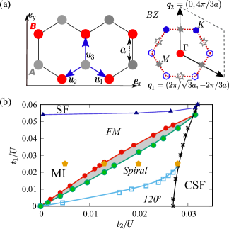
Figure 1: (a) Honeycomb lattice with $\bm{u}_{i}$ – vectors between first neighbor sites and the first Brillouin zone with explicitly shown $\bm{\Gamma}$, $\bm{K}$ and $\bm{M}$ points. (b) Phase diagram of the BKMH model obtained using B-DMFT containing Mott insulator (MI), uniform superfluid (SF) and chiral superfluid (CSF) phases with different regimes of the MI phase marked in italic. The central gray region corresponds to the states with no coplanar order. Parameters $U_{\uparrow\downarrow}/U=0.5,\ \mu/U_{\uparrow\downarrow}=0.5$, lattice of 96 sites. ”Pentagons” mark parameter values that we further explore in Fig. 2(a-d).

I. B-DMFT on BKMH model. The ground-state phase diagram of the BKMH model obtained from B-DMFT Georges et al. (1996); Byczuk and Vollhardt (2008); Hu and Tong (2009); Hubener et al. (2009); Anders et al. (2010) is shown in Fig. 1(b). In order to address unusual states that break translational symmetry, we use real-space B-DMFT Li et al. (2011); He et al. (2012, 2015); sup . Local effective problems represented by the Anderson impurity model are solved using exact diagonalization sup . As found for the bosonic Haldane model with same filling Vasić et al. (2015), three phases are competing: a uniform superfluid (SF), a chiral superfluid (CSF) and a Mott insulator (MI) (they are sorted out from the behaviors of the order parameter $\braket{b_{\sigma,\bm{r}_{i}}}$ and the local currents $J^{\sigma}_{ij}=\mathfrak{Im}\braket{b^{\dagger}_{\sigma,\bm{r}_{i}}b_{\sigma,\bm{r}_{j}}}$ sup ).

We now focus on the MI phase. As shown in Fig. 1(b), the system enters the Mott phase when intra-species ($U$) and inter-species ($U_{\uparrow\downarrow}$) interactions become strong enough. Applying standard perturbation theory Kuklov and Svistunov (2003), one rewrites the Hamiltonian (Emergent Chiral Spin State in the Mott Phase of a Bosonic Kane-Mele-Hubbard Model) in terms of pseudo spin-$1/2$ operators $S^{+}_{\bm{r}_{i}}=S^{x}_{\bm{r}_{i}}+iS^{y}_{\bm{r}_{i}}=b^{\dagger}_{\uparrow,\bm{r}_{i}}b_{\downarrow,\bm{r}_{i}}$, $S^{-}_{\bm{r}_{i}}=S^{x}_{\bm{r}_{i}}-iS^{y}_{\bm{r}_{i}}=b^{\dagger}_{\downarrow,\bm{r}_{i}}b_{\uparrow,\bm{r}_{i}}$ and $S^{z}_{\bm{r}_{i}}=(n_{\uparrow,\bm{r}_{i}}-n_{\downarrow,\bm{r}_{i}})/2$ as follows:

$$H= -\sum\limits_{\Braket{ij}}\left[J_{1}\left(S_{\bm{r}_{i}}^{+}S_{\bm{r}_{j}}^{-}+\textrm{h.c.}\right)-K_{1}S_{\bm{r}_{i}}^{z}S_{\bm{r}_{j}}^{z}\right]$$

$$+\sum\limits_{\Braket{\Braket{ik}}}\left[J_{2}\left(S_{\bm{r}_{i}}^{+}S_{\bm{r}_{k}}^{-}+\textrm{h.c.}\right)+K_{2}S_{\bm{r}_{i}}^{z}S_{\bm{r}_{k}}^{z}\right]\;,$$ (2)

where $J_{i}=t_{i}^{2}/U_{\uparrow\downarrow}$ and $K_{i}=t_{i}^{2}\left(1/U_{\uparrow\downarrow}-2/U\right)$. We observe that the spin-$1/2$ frustrated XY model is realized when $U=2U_{\uparrow\downarrow}$ (for which $K_{i}=0$). Frustration is associated with the positive sign of the $J_{2}$-term, which combines the sign of the bosonic exchange and the phase of $\pi$ accumulated in the hoppings between second neighbors. The fermionic Kane-Mele model does not include such frustrating terms Young et al. (2008); Rachel and Le Hur (2010). The properties of this effective XY model depend only on the ratio $J_{2}/J_{1}=\left(t_{2}/t_{1}\right)^{2}$. In the classical limit, a coplanar ansatz Rastelli et al. (1979); Fouet et al. (2001); sup provides the following phase diagram: the ferromagnetic phase is stable for $J_{2}/J_{1}\leq 1/6$, above which degenerate incommensurate spiral waves become energetically favoured. Their wave-vectors leave on closed contours in the Brillouin zone. In the case of the Heisenberg model, quantum fluctuations were predicted to lift this degeneracy via an order by disorder mechanism Mulder et al. (2010).

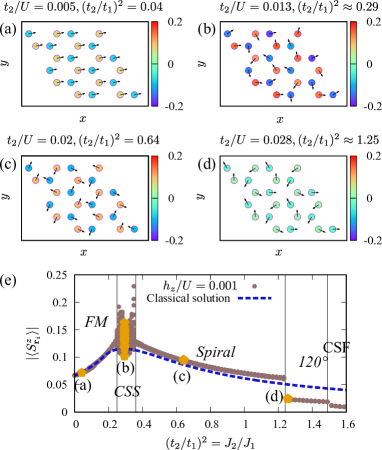
Figure 2: Results of the B-DMFT for different values of $\left(t_{2}/t_{1}\right)^{2}=J_{2}/J_{1}$ for $h_{z}/U=10^{-3}$, $U_{\uparrow\downarrow}/U=0.5,t_{1}/U=0.025$ on a lattice of 24 sites. (a-d) Different spin configurations. The color palette gives $\braket{S^{z}_{\bm{r}_{i}}}$, while arrows depict ordering in the $xy$-plane. (a) Uniform state with FM ordering; (b) CSS (chiral spin state) with no coplanar order; (c) A configuration of spiral states, in which each pseudo spin is aligned with only one of its three first neighbors and anti-aligned with two of its six second neighbors; (d) A $120^{\circ}$ configuration. (e) Absolute value of $\left|\braket{S^{z}_{\bm{r}_{i}}}\right|$. For each ratio $(t_{2}/t_{1})^{2}$ we plot the result for all 24 sites and compare it to the classical solution. ”Pentagons” mark results presented in (a-d). Note that for finite values of $h_{z}$ the border between the $120^{\circ}$ Mott state and CSF is slightly shifted in favour of the Mott state.

Deviations from this classical picture are already captured by B-DMFT in the BKMH model. In Fig. 2(a-d), we study the local coplanar spin ordering (arrows), in the presence of an external staggered magnetic field $h_{z}$, breaking the parity $\mathcal{P}$ symmetry (reflection which maps the sublattice $A$ to the sublattice $B$):

$$H_{z}=h_{z}\Big{(}\sum\limits_{i\in{A}}S^{z}_{\bm{r}_{i}}-\sum\limits_{j\in{B}}S^{z}_{\bm{r}_{j}}\Big{)}\;.$$ (3)

It corresponds to a staggered chemical potential in the boson language and we will understand its role hereafter. We directly infer some of the ordered phases: at low $J_{2}/J_{1}$, all spins are aligned in a ferromagnetic (FM) order, while at large $J_{2}/J_{1}$, we recover a $120^{\circ}$ spiral order. For $U_{\uparrow\downarrow}/U=0.5,t_{1}/U=0.025$ in the range $0.36\lesssim J_{2}/J_{1}\lesssim 1.23$ we observe a different configuration of spiral waves (Fig. 2(c)). In addition, we find an exotic intermediate regime when $0.25\lesssim J_{2}/J_{1}\lesssim 0.36$ (we notice that positions of phase boundaries are affected by $h_{z}$), characterized by a chiral spin state (CSS) (this definition will be justified later) with no coplanar magnetic order (Fig. 2(b)). This is reminiscent of the debated intermediate phase found in numerical studies on the XY spin model Varney et al. (2011, 2012); Carrasquilla et al. (2013); Di Ciolo et al. (2014); Nakafuji and Ichinose (2017); Zhu et al. (2013b); Zhu and White (2014); Bishop et al. (2014). On one hand, density matrix renormalization group Zhu et al. (2013b); Zhu and White (2014) and coupled cluster method Bishop et al. (2014) results evidenced an antiferromagnetic Ising ordering along the $z$-axis, breaking $\mathcal{P}$ while preserving translational invariance. On the other hand, this observation was not reported in ED Varney et al. (2011, 2012) nor variational Monte-Carlo Carrasquilla et al. (2013); Di Ciolo et al. (2014); Nakafuji and Ichinose (2017) analyses, raising questions about the exact nature of this intermediate phase.

Mapping the model onto a fermionic one and performing a mean-field analysis Sedrakyan et al. (2015); sup , it was proposed that an intermediate frustration stabilizes a phase with spontaneously broken parity $\mathcal{P}$ and time-reversal $\mathcal{T}$ symmetries. This phase is characterized by antiferromagnetic correlations and ChS fluxes staggered within the unit cell as in the celebrated Haldane model Haldane (1988) and the authors suggested that it realizes the chiral spin liquid state of Kalmeyer-Laughlin Kalmeyer and Laughlin (1987, 1989). In this context, we plot in Fig. 2(e), the response for the magnetization $\braket{S^{z}_{\bm{r}_{i}}}$ with respect to the field $h_{z}$. All phases except the CSS are characterized by a trivial response to the perturbation: $\braket{S^{z}_{\bm{r}_{i}}}\sim h_{z}$, whereas $\braket{S^{z}_{\bm{r}_{i}}}$ is strongly fluctuating in the CSS (however we do not observe spontaneous symmetry breaking with B-DMFT). These results cannot be explained in the context of a simple coplanar ansatz, but could be related to a breaking of the degeneracy between two mean-field solutions in the ChS field theory description sup .

II. ED on frustrated XY model. We complete the study of the effective frustrated XY model using ED and previously unaddressed probes such as the responses to $\mathcal{P}$ and $\mathcal{T}$ breaking perturbations and the topological description of the ground-state. We consider lattices of $24-32$ sites, with periodic boundary conditions, and fixed total magnetization $S^{z}_{\textrm{Tot}}=0$ if not stated otherwise. First, we determine the phase boundaries using the fidelity metric Zanardi and Paunković (2006); Gu (2010); Varney et al. (2010); sup $g$. The phase diagram of the XY model deduced from the ED calculations is given in Fig. 3(a). In agreement with the B-DMFT analysis and previous numerical studies, we observe three phase transitions at $J_{2}/J_{1}\approx 0.21,0.36$ and $1.32$. Small deviations from the B-DMFT results could be due to a finite size of ED clusters or non-perturbative interaction effects ($XY$ model does not describe correctly the physics of the Mott phase when $t_{i}/U$ are not small enough). The nature of the phases detected with the ED is verified by looking at the coplanar static structure factor

$$S_{\textrm{Spiral}}\left(\bm{q}\right)=2\sum\limits_{i,j\in A}e^{i\bm{q}\cdot\left(\bm{r}_{i}-\bm{r}_{j}\right)}\braket{S^{x}_{\bm{r}_{i}}S^{x}_{\bm{r}_{j}}}\;.$$ (4)

Spiral waves display a maximum of $S_{\textrm{Spiral}}(\bm{q})$ at some wave-vector(s) $\bm{q}$ in the first Brillouin zone. In the bosonic language, this is interpreted as a macroscopic occupation of the corresponding momentum state(s). We observe sup that the phase in the region $J_{2}/J_{1}\lesssim 0.21$ corresponds to the FM order since $S_{\textrm{Spiral}}\left(\bm{q}\right)$ has a peak at $\bm{q}=\bm{\Gamma}$. The phase at $0.36\lesssim J_{2}/J_{1}\lesssim 1.32$ corresponds to a spiral wave with collinear order (structure factor has maxima at three $\bm{M}$ points) as expected from the order by disorder mechanism. At $1.32\lesssim J_{2}/J_{1}$ the ground-state is the $120^{\circ}$ order spiral wave (structure factor has a peak at two Dirac points $\bm{K}$). In the intermediate frustration regime ($0.21\lesssim J_{2}/J_{1}\lesssim 0.36$) the coplanar static structure factor is flat in the reciprocal space and we expect the ground-state to be disordered in the $xy$-plane. Notice that the ground-state in all phases is located in the same sector of the total momentum at point $\bm{\Gamma}$. Based on the ChS field theory predictions, the order by disorder arguments and numerical observations, the CSS – collinear order and collinear order – $120^{\circ}$ order phase transitions are expected to be of the first order, whereas the FM – CSS phase transition – of the second order.

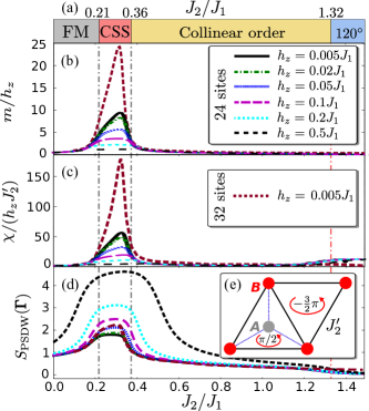
Figure 3: (a) Phase diagram of the frustrated XY model from ED. (b-d) Variation of the observables with the dimensionless parameter $J_{2}/J_{1}$ for different values of $h_{z}$, with $J^{\prime}_{2}=0.01J_{1}$, on a lattice of $6\times 2$ unit cells. (b) Difference of the average Ising magnetization on two sublattices $m$. (c) Scalar spin chirality $\chi$. (d) Pseudo-spin density wave structure factor $S_{\text{PSDW}}(\bm{\Gamma})$. (e) Schematic representation of the perturbation term $H_{J^{\prime}_{2}}$.

As for the B-DMFT study, we analyze the linear response to external perturbations breaking $\mathcal{P}$ and $\mathcal{T}$ symmetries. We are interested in the relative magnetization between the two sublattices $m=\Braket{m_{\bm{r}_{i}}}=\Braket{S^{z}_{\bm{r}_{i}}-S^{z}_{\bm{r}_{i}+\bm{u}_{3}}}$, as well as the scalar spin chirality $\chi=\Braket{\bm{S}_{\bm{r}_{i}}\cdot\left(\bm{S}_{\bm{r}_{i}+\bm{u}_{1}}\times\bm{S}_{\bm{r}_{i}+\bm{u}_{2}}\right)}$. Here we suppose that $i\in A$ and $\bm{u}_{i}$ are vectors between first neighbor sites defined in Fig. 1(a). When calculating the chirality $\chi$, we add a perturbation corresponding to the second-neighbor hopping of the Haldane model, of amplitude $J^{\prime}_{2}$ and phase $\pi/2$ (as shown in Fig. 3(e)):

$$H_{J^{\prime}_{2}}=J^{\prime}_{2}\sum\limits_{\Braket{\Braket{ik}}}\big{(}e^{\pm i\pi/2}S_{\bm{r}_{i}}^{+}S_{\bm{r}_{k}}^{-}+\textrm{h.c.}\big{)}\;.$$ (5)

We are interested in the limit $h_{z},J^{\prime}_{2}\ll J_{1}$. Results of the ED calculations are presented in Figs. 3(b-c). The CSS reveals itself by sharp responses to such external fields. Moreover, the renormalized quantities $m/h_{z}$ and $\chi/(h_{z}J^{\prime}_{2})$ tend to diverge in weak-coupling limit, giving a strong indication for spontaneous symmetry breaking. This justifies our definition of the CSS, which properties can be observed experimentally by tracking on-site populations of bosons $n_{\sigma,\bm{r}_{i}}$ and currents $J^{\sigma}_{ij}=\mathfrak{Im}\Braket{b^{\dagger}_{\sigma,\bm{r}_{i}}b_{\sigma,\bm{r}_{j}}}$Atala et al. (2014). One can probe the antiferromagnetic ordering without breaking $\mathcal{P}$ and $\mathcal{T}$ by calculating the pseudo-spin density wave (PSDW) structure factor Varney et al. (2011, 2012):

$$S_{\textrm{PSDW}}(\bm{q})=\!\!\sum\limits_{i,j}e^{i\bm{q}\cdot\left(\bm{r}_{i}-\bm{r}_{j}\right)}\Braket{m_{\bm{r_{i}}}m_{\bm{r_{j}}}}.$$

We observe in Fig. 3(d) that $S_{\textrm{PSDW}}(\bm{q})$ has a peak at $\bm{q}=\bm{\Gamma}$ in the intermediate frustration regime. These features are hardly affected by moderate Ising interactions $K_{i}/J_{1}\sim 0.1$ in Eq. (Emergent Chiral Spin State in the Mott Phase of a Bosonic Kane-Mele-Hubbard Model) Li et al. (2014).

The observed spin configuration of the CSS could describe the chiral spin liquid of Kalmeyer and Laughlin Kalmeyer and Laughlin (1987, 1989). Yet, we know that chiral spin liquids are characterized by a topological degeneracy in the thermodynamic limit on a compact space with genus $G$ Wen et al. (1989); Wen (1989, 1995). This property can be checked using ED in a system with periodic boundaries: as $G=1$ for a torus, one should have a four-fold degenerate ground-state with two topological degeneracies per chirality sector. Still, because of finite size effects, one only expects an approximate degeneracy in simulations.

In Fig. 4(a-b), we show the low-energy spectrum as a function of $J_{2}/J_{1}$, resolved in different sectors of total momentum $\bm{Q}$. As mentioned previously, the ground-state always belongs to the sector $\bm{Q}=\bm{\Gamma}$. In the intermediate frustration regime, we clearly observe the onset of a doubly-degenerate ground-state manifold, well separated from higher energy states. The first excited state has the same momentum $\bm{Q}=\bm{\Gamma}$, but lies in the opposite sector of spin-inversion symmetry $S^{z}_{\bm{r}_{i}}\rightarrow-S^{z}_{\bm{r}_{i}}$ or reflection symmetry (that coincides with $\mathcal{P}$) for some particular lattices. Low-lying excited state also moves away in energy when the perturbations $H_{z}$ and $H_{J^{\prime}_{2}}$ are switched on.

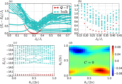
Figure 4: ED calculations of the low energy spectra as a function of $J_{2}/J_{1}$ (a) on a lattice of $4\times 3$ unit cells for various $S^{z}_{\text{Tot}}$; (b) on a lattice of $4\times 4$ unit cells in the $S^{z}_{\text{Tot}}=0$ sector only. (c) Low energy spectrum as a function of the twist angle $\theta_{1}$ for $J_{2}/J_{1}=0.3$ and $\theta_{2}=0$ on a lattice of $4\times 3$ unit cells. (d) Berry curvature calculated using the non-abelian formalism resulting in a vanishing Chern number shown for $J_{2}/J_{1}=0.3$, $h_{z}/J_{1}=J_{2}^{\prime}/J_{1}=0.02$ on a lattice of $4\times 3$ unit cells.

We probe the robustness of the low energy quasi-degenerate state sector by performing the Laughlin’s gedanken experiment and pumping a quantum of magnetic flux through one of the non-trivial loops of the torus Laughlin (1981, 1983); Thouless (1989). Numerically, this is achieved using twisted boundary conditions in a translational symmetry preserving manner. The results are given in Fig. 4(c). We observe that the same states in the sector $\bm{Q}=\bm{\Gamma}$ are non-trivially gapped for all twists. For a pumping of a single flux quantum we could not observe a crossing of states in the ground-state manifold, that however does not imply that the manifold is topologically trivial Wang et al. (2011); Hickey et al. (2016); Kumar et al. (2016a). The topological nature of the ground-state manifold is unambiguously determined by calculating the Chern number Niu et al. (1985); Kohmoto (1985); Hatsugai (2004, 2005):

$$C=\frac{1}{2\pi}\int\limits_{0}^{2\pi}\int\limits_{0}^{2\pi}B(\theta_{1},\theta_{2})\textrm{d}\theta_{1}\textrm{d}\theta_{2}\;.$$ (6)

Here $\theta_{1}$ and $\theta_{2}$ are two angles of twisted boundary conditions and $B(\theta_{1},\theta_{2})$ is the Berry curvature Berry (1984). We notice that two phases $\theta_{i}$ ($i=1,2$) introduced in the spin language would correspond to four phases $\theta^{\sigma}_{i}$ in the language of bosons of the BKMH model, for which the spin component $\theta^{\uparrow}_{i}-\theta^{\downarrow}_{i}=\theta_{i}$ is fixed and the $U(1)$ component $\theta^{\uparrow}_{i}+\theta^{\downarrow}_{i}$ is free Fu and Kane (2006). Since the two quasi degenerate ground-states lie in the same symmetry sector and cannot be separated unless twists are trivial (reflection and spin-inversion symmetry can not be used with twisted boundary conditions), we evaluate the Berry curvature using the gauge-invariant non-abelian formulation Yu et al. (2011); Shapourian and Clark (2016); Kumar et al. (2016b): $B(\theta_{1},\theta_{2})\delta\theta_{1}\delta\theta_{2}=\mathfrak{Im}\ln\mathfrak{Det}\left(\mathcal{M}(\theta_{1},\theta_{2})\right)$, where elements of the matrix $\mathcal{M}$ are obtained as follows:

$$\mathcal{M}_{ij}(\theta_{1},\theta_{2}) =\Braket{\phi_{i}(\theta_{1},\theta_{2})}{\phi_{\mu_{1}}(\theta_{1}+\delta\theta_{1},\theta_{2})}$$

$$\times\Braket{\phi_{\mu_{1}}(\theta_{1}+\delta\theta_{1},\theta_{2})}{\phi_{\mu_{2}}(\theta_{1}+\delta\theta_{1},\theta_{2}+\delta\theta_{2})}$$

$$\times\Braket{\phi_{\mu_{2}}(\theta_{1}+\delta\theta_{1},\theta_{2}+\delta\theta_{2})}{\phi_{\mu_{3}}(\theta_{1},\theta_{2}+\delta\theta_{2})}$$

$$\times\Braket{\phi_{\mu_{3}}(\theta_{1},\theta_{2}+\delta\theta_{2})}{\phi_{j}(\theta_{1},\theta_{2})}\;.$$ (7)

Here $\delta\theta_{1}$ and $\delta\theta_{2}$ refer to the numerical mesh along the $\theta_{1}$ and $\theta_{2}$. $i,j,\mu_{i}=1,2$ are indices of states $\Ket{\phi_{1}}$ and $\Ket{\phi_{2}}$ in the ground-state manifold and the summation over $\mu_{i}$ is implicit. In Fig. 4(d), we show a typical shape of the Berry curvature. We find that the Chern number is zero in the intermediate frustration regime. This result suggests that the intermediate phase in the frustrated XY model is most likely to be a CSS with no topological order, as suggested in Refs. Zhu et al., 2013b; Zhu and White, 2014; Bishop et al., 2014 and not the Kalmeyer-Laughlin state, with gauge fluctuations beyond the mean-field solution making the phase topologically trivial as in the fermionic Kane-Mele model case Rachel and Le Hur (2010); Wu et al. (2012); Hohenadler et al. (2012).

To conclude, we studied the phase diagram of the bosonic Kane-Mele-Hubbard model on the honeycomb lattice. We have shown that an effective frustrated XY model appears in the Mott insulator phase. This model possesses an intermediate frustration regime with a non-trivial chiral spin state, which breaks both $\mathcal{P}$ and $\mathcal{T}$ symmetries. It displays a finite scalar spin chirality order and an antiferromagnetic ordering between first-neighbor sites, while remaining translationally invariant. Measuring the Chern number associated with this state reveals its non-topological nature.

We thank Loïc Herviou, Grégoire Misguich, Stephan Rachel, Cécile Repellin, Tigran Sedrakyan for insightful discussions. This work has also benefitted from discussions at CIFAR meetings in Canada and Société Française de Physique.

Support by the Deutsche Forschungsgemeinschaft via DFG FOR 2414, DFG SPP 1929 GiRyd, and the high-performance computing center LOEWE-CSC is gratefully acknowledged. This work was supported in part by DAAD (German Academic and Exchange Service) under project BKMH. I. V. acknowledges support by the Ministry of Education, Science, and Technological Development of the Republic of Serbia under projects ON171017 and BKMH, and by the European Commission under H2020 project VI-SEEM, Grant No. 675121. Numerical simulations were partly run on the PARADOX supercomputing facility at the Scientific Computing Laboratory of the Institute of Physics Belgrade. K. L. H. acknowledges support from Labex PALM.

Supplemental Material: Emergent Chiral Spin State in the Mott Phase of a Bosonic Kane-Mele-Hubbard Model

I B-DMFT details

For completeness, in this Section we briefly describe the B-DMFT method along the lines of references Hubener et al. (2009); Snoek and Hofstetter (2013); Anders et al. (2010); Li et al. (2011). In particular, in order to be able to address exotic states that break translational invariance, we implement real-space B-DMFT Snoek and Hofstetter (2013); Li et al. (2011); He et al. (2012, 2015). The essence of DMFT is mapping of the full lattice model onto a set of local models whose parameters are determined through a self-consistency condition. The self-consistency is imposed on the level of single–particle Green’s functions that can be written in the Nambu notation as

$$G_{ij}(\tau,\eta)\equiv G_{ij}(\tau-\eta)=-T_{\tau,\eta}\left\langle\left(\begin{array}[]{cccc}b_{\uparrow,\bm{r}_{i}}(\tau)b_{\uparrow,\bm{r}_{j}}^{\dagger}(\eta)&b_{\uparrow,\bm{r}_{i}}(\tau)b_{\uparrow,\bm{r}_{j}}(\eta)&b_{\uparrow,\bm{r}_{i}}(\tau)b_{\downarrow,\bm{r}_{j}}^{\dagger}(\eta)&b_{\uparrow,\bm{r}_{i}}(\tau)b_{\downarrow,\bm{r}_{j}}(\eta)\\ b_{\uparrow,\bm{r}_{i}}^{\dagger}(\tau)b_{\uparrow,\bm{r}_{j}}^{\dagger}(\eta)&b_{\uparrow,\bm{r}_{i}}^{\dagger}(\tau)b_{\uparrow,\bm{r}_{j}}(\eta)&b_{\uparrow,\bm{r}_{i}}^{\dagger}(\tau)b_{\downarrow,\bm{r}_{j}}^{\dagger}(\eta)&b_{\uparrow,\bm{r}_{i}}^{\dagger}(\tau)b_{\downarrow,\bm{r}_{j}}(\eta)\\ b_{\downarrow,\bm{r}_{i}}(\tau)b_{\uparrow,\bm{r}_{j}}^{\dagger}(\eta)&b_{\downarrow,\bm{r}_{i}}(\tau)b_{\uparrow,\bm{r}_{j}}(\eta)&b_{\downarrow,\bm{r}_{i}}(\tau)b_{\downarrow,\bm{r}_{j}}^{\dagger}(\eta)&b_{\downarrow,\bm{r}_{i}}(\tau)b_{\downarrow,\bm{r}_{j}}(\eta)\\ b_{\downarrow,\bm{r}_{i}}^{\dagger}(\tau)b_{\uparrow,\bm{r}_{j}}^{\dagger}(\eta)&b_{\downarrow,\bm{r}_{i}}^{\dagger}(\tau)b_{\uparrow,\bm{r}_{j}}(\eta)&b_{\downarrow,\bm{r}_{i}}^{\dagger}(\tau)b_{\downarrow,\bm{r}_{j}}^{\dagger}(\eta)&b_{\downarrow,\bm{r}_{i}}^{\dagger}(\tau)b_{\downarrow,\bm{r}_{j}}(\eta)\end{array}\right)\right\rangle\;.$$ (8)

In the following we express the Green’s functions in terms of Matsubara frequencies $\omega_{n}=2\pi n/\beta$, where $\beta$ is the inverse temperature (in the zero temperature limit $\beta\rightarrow\infty$) and $G_{ij}(i\omega_{n})=\int\,d{\tau}\exp(i\omega_{n}\tau)G_{ij}(\tau)$.

In real-space B-DMFT we decompose the full lattice problem into a set of local single-site effective problems. The approximation is such that local correlations are fully taken into account, while non-local correlations are treated at the mean-field level. At each site $i$, we attach a bath described by orbital degrees of freedom. The effective local Hamiltonian is given by a bosonic Anderson impurity (AI) model Snoek and Hofstetter (2013)

$$\mathcal{H}^{\mathrm{AI}}_{i} = \sum_{l=0}^{L}\left[\varepsilon_{l}a_{l}^{\dagger}a_{l}+\sum_{\sigma}\left(V_{l,\sigma}a_{l}^{\dagger}b_{\sigma,\bm{r}_{i}}+V_{l,\sigma}^{*}a_{l}b_{\sigma,\bm{r}_{i}}^{\dagger}+W_{l,\sigma}a_{l}b_{\sigma,\bm{r}_{i}}+W_{l,\sigma}^{*}a_{l}^{\dagger}b_{\sigma,\bm{r}_{i}}^{\dagger}\right)\right]$$ (9)

$$+ \sum_{\sigma}\left(-\psi_{\sigma,\bm{r}_{i}}^{\mathrm{AI}*}b_{\sigma,\bm{r}_{i}}-\psi_{\sigma,\bm{r}_{i}}^{\mathrm{AI}}b^{\dagger}_{\sigma,\bm{r}_{i}}+\frac{U}{2}n_{\sigma,\bm{r}_{i}}(n_{\sigma,\bm{r}_{i}}-1)-\mu_{\sigma}n_{\sigma,\bm{r}_{i}}\right)+U_{\uparrow\downarrow}n_{\uparrow,\bm{r}_{i}}n_{\downarrow,\bm{r}_{i}},$$

where the index $l$ labels the Anderson orbitals with energies $\varepsilon_{l}$ and we allow for complex values of the Anderson parameters $V_{l,\sigma}$ and $W_{l,\sigma}$ that couple orbital degrees of freedom with impurity atoms. We use $L=4$; we check that results are the same for $L=5$ and $6$. Local interaction terms proportional to $U$ and $U_{\uparrow\downarrow}$ come directly from the initial lattice model and, as we work in the grand canonical ensemble, we introduce chemical potentials $\mu_{\sigma}\equiv\mu$. We define hybridization functions of the Anderson impurity model as

$$\Delta_{11}^{\nu\mu}(i\omega_{n}) = \sum_{l}\left(\frac{V_{l,\nu}^{*}V_{l,\mu}}{\epsilon_{l}-i\omega_{n}}+\frac{W_{l,\nu}^{*}W_{l,\mu}}{\epsilon_{l}+i\omega_{n}}\right),$$ (10)

$$\Delta_{22}^{\nu\mu}(i\omega_{n}) = \sum_{l}\left(\frac{W_{l,\mu}^{*}W_{l,\nu}}{\epsilon_{l}-i\omega_{n}}+\frac{V_{l,\mu}^{*}V_{l,\nu}}{\epsilon_{l}+i\omega_{n}}\right),$$ (11)

$$\Delta_{12}^{\nu\mu}(i\omega_{n}) = \sum_{l}\left(\frac{V_{l,\nu}^{*}W^{*}_{l,\mu}}{\epsilon_{l}-i\omega_{n}}+\frac{V_{l,\mu}^{*}W^{*}_{l,\nu}}{\epsilon_{l}+i\omega_{n}}\right),$$ (12)

$$\Delta_{21}^{\nu\mu}(i\omega_{n}) = \sum_{l}\left(\frac{V_{l,\mu}W_{l,\nu}}{\epsilon_{l}-i\omega_{n}}+\frac{V_{l,\nu}W_{l,\mu}}{\epsilon_{l}+i\omega_{n}}\right),$$ (13)

and introduce a $4\times 4$ matrix $\Delta(i\omega_{n})$ as

$$\Delta(i\omega_{n})\equiv\left(\begin{array}[]{cccc}\Delta_{11}^{\uparrow\uparrow}&\Delta_{12}^{\uparrow\uparrow}&\Delta_{11}^{\uparrow\downarrow}&\Delta_{12}^{\uparrow\downarrow}\\ \Delta_{21}^{\uparrow\uparrow}&\Delta_{22}^{\uparrow\uparrow}&\Delta_{21}^{\uparrow\downarrow}&\Delta_{22}^{\uparrow\downarrow}\\ \Delta_{11}^{\downarrow\uparrow}&\Delta_{12}^{\downarrow\uparrow}&\Delta_{11}^{\downarrow\downarrow}&\Delta_{12}^{\downarrow\downarrow}\\ \Delta_{21}^{\downarrow\uparrow}&\Delta_{22}^{\downarrow\uparrow}&\Delta_{21}^{\downarrow\downarrow}&\Delta_{22}^{\downarrow\downarrow}\end{array}\right).$$ (14)

The following relations for the hybridization functions hold true:

$$\Delta_{22}^{\uparrow\uparrow}(i\omega_{n})=\Delta_{11}^{{\uparrow\uparrow}*}(i\omega_{n}),\quad\Delta_{21}^{\uparrow\uparrow}(i\omega_{n})=\Delta_{12}^{{\uparrow\uparrow}*}(i\omega_{n}),\quad\Delta_{22}^{\downarrow\downarrow}(i\omega_{n})=\Delta_{11}^{{\downarrow\downarrow}*}(i\omega_{n}),\quad\Delta_{21}^{\downarrow\downarrow}(i\omega_{n})=\Delta_{12}^{{\downarrow\downarrow}*}(i\omega_{n}),$$

$$\Delta_{22}^{\uparrow\downarrow}(i\omega_{n})=\Delta_{11}^{{\uparrow\downarrow}*}(i\omega_{n}),\quad\Delta_{21}^{\uparrow\downarrow}(i\omega_{n})=\Delta_{12}^{{\uparrow\downarrow}*}(i\omega_{n}),\quad\Delta_{22}^{\downarrow\uparrow}(i\omega_{n})=\Delta_{11}^{{\downarrow\uparrow}*}(i\omega_{n}),\quad\Delta_{21}^{\downarrow\uparrow}(i\omega_{n})=\Delta_{12}^{{\downarrow\uparrow}*}(i\omega_{n}).$$ (15)

The terms $\psi_{\sigma,\bm{r}_{i}}^{\mathrm{AI}}$ used in Eq. (9) incorporate a correction with respect to the mean–field result and they read Snoek and Hofstetter (2013):

$$\psi_{\uparrow,\bm{r}_{i}}^{\mathrm{AI}} = \sum_{j}t_{\uparrow,ij}\phi_{\uparrow,\bm{r}_{j}}-\phi_{\uparrow,\bm{r}_{i}}^{*}\Delta_{21}^{\uparrow\uparrow}(0)-\phi_{\downarrow,\bm{r}_{i}}^{*}\Delta_{21}^{\downarrow\uparrow}(0)-\phi_{\uparrow,\bm{r}_{i}}\Delta_{11}^{\uparrow\uparrow}(0)-\phi_{\downarrow,\bm{r}_{i}}\Delta_{11}^{\downarrow\uparrow}(0),$$ (16)

$$\psi_{\downarrow,\bm{r}_{i}}^{\mathrm{AI}} = \sum_{j}t_{\downarrow,ij}\phi_{\downarrow,\bm{r}_{j}}-\phi_{\uparrow,\bm{r}_{i}}^{*}\Delta_{21}^{\uparrow\downarrow}(0)-\phi_{\downarrow,\bm{r}_{i}}^{*}\Delta_{21}^{\downarrow\downarrow}(0)-\phi_{\uparrow,\bm{r}_{i}}\Delta_{11}^{\uparrow\downarrow}(0)-\phi_{\downarrow,\bm{r}_{i}}\Delta_{11}^{\downarrow\downarrow}(0),$$ (17)

where the condensate order parameters are defined as

$$\phi_{\sigma,\bm{r}_{i}}=\langle b_{\sigma,\bm{r}_{i}}\rangle,$$ (18)

and $t_{\sigma,ij}$ are hopping amplitudes of the two species defined in the initial lattice model.

By exact diagonalization of the local model (9) we obtain the values of the local Green’s functions. From here, the local self–energy is obtained from the local Dyson equation

$$(G^{\mathrm{AI}})^{-1}_{ii}(i\omega_{n})=\left(\begin{array}[]{cccc}i\omega_{n}+\mu&&&\\ &-i\omega_{n}+\mu&&\\ &&i\omega_{n}+\mu&\\ &&&-i\omega_{n}+\mu\end{array}\right)+\Delta(i\omega_{n})-\Sigma_{i}^{\mathrm{AI}}.$$ (19)

The approximate real-space Dyson equation takes the following form:

$$G^{-1}_{ij,\mathrm{latt}}(i\omega_{n})=\left(\begin{array}[]{cccc}\!\!\left(i\omega_{n}+\mu\right)\delta_{ij}+t_{\uparrow,ij}&&&\\ \!&\!\!\left(-i\omega_{n}+\mu\right)\delta_{ij}+t^{*}_{\uparrow,ij}\!\!&\!&\!\\ \!&\!&\!\!\left(i\omega_{n}\!+\!\mu\right)\delta_{ij}+t_{\downarrow,ij}&\!\!\\ \!&\!&\!&\left(-i\omega_{n}\!+\!\mu\right)\delta_{ij}+t^{*}_{\downarrow,ij}\\ \end{array}\right)-\delta_{ij}\Sigma_{i}^{\mathrm{AI}},$$ (20)

where we approximate the self–energy by a local contribution from Eq. (19). The last step represents the main approximation of DMFT. Finally, we need a criterion to set the values of the parameters $\varepsilon_{l}$, $V_{l,\sigma}$ and $W_{l,\sigma}$ in Eq. (9). To this end, a condition is imposed on the hybridization functions (13). These functions should be optimized such that the two Dyson equations, (19) and (20), yield the same values of the local Green’s functions. In practice, we iterate a self–consistency loop to fulfill this condition, starting from arbitrary initial values. At the same time we impose a simple self consistency on the local condensate order parameters $\phi_{\sigma,\bm{r}_{i}}$.

Once that the self-consistency is achieved and values of Anderson parameters $\varepsilon_{l},V_{l,\sigma}$ and $W_{l,\sigma}$ are fixed, by solving the local model (9) we obtain results for local condensate order parameters (18) and the expectation values of the pseudo spin operators

$$\langle S^{x}_{{\mathbf{r}}_{i}}\rangle = \langle b_{\uparrow,\bm{r}_{i}}^{\dagger}b_{\downarrow,\bm{r}_{i}}+b_{\downarrow,\bm{r}_{i}}^{\dagger}b_{\uparrow,\bm{r}_{i}}\rangle/2,$$ (21)

$$\langle S^{y}_{{\mathbf{r}}_{i}}\rangle = i\langle b_{\uparrow,\bm{r}_{i}}^{\dagger}b_{\downarrow,\bm{r}_{i}}-b_{\downarrow,\bm{r}_{i}}^{\dagger}b_{\uparrow,\bm{r}_{i}}\rangle/2,$$ (22)

$$\langle S^{z}_{{\mathbf{r}}_{i}}\rangle = \langle b_{\uparrow,\bm{r}_{i}}^{\dagger}b_{\uparrow,\bm{r}_{i}}-b_{\downarrow,\bm{r}_{i}}^{\dagger}b_{\downarrow,\bm{r}_{i}}\rangle/2.$$ (23)

We work with a finite lattice consisting of 96 sites and periodic boundary conditions that provide a proper sampling of the Brillouin zone that includes its corners Varney et al. (2010). The values of the chemical potential terms in Eq. (9) are fixed to $\mu_{\sigma}=U_{\uparrow\downarrow}/2$.

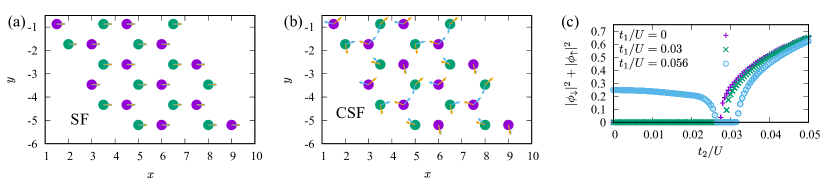
Figure 5: Color maps: Real-space distribution of condensate order parameters of the two bosonic species in (a) uniform superfluid (SF) ($t_{1}/U=0.056,t_{2}/U=0.005,U_{\uparrow\downarrow}/U=0.5,\mu/U_{\uparrow\downarrow}=0.5$), and (b) chiral superfluid (CSF) ($t_{1}/U=0.018,t_{2}/U=0.032,U_{\uparrow\downarrow}/U=0.5,\mu/U_{\uparrow\downarrow}=0.5$). Local condensate order parameters are aligned in the SF. In contrast, they exhibit $2\pi/3$ winding in the CSF. The ”winding direction” is opposite for the two species and for the two sublattices, implying that for each sublattice the two species condense in the two different Dirac points. The choice of the Dirac points is opposite for the two sublattices. (c) The condensate order parameters as a function of $t_{2}/U$ for several values of $t_{1}/U$.

Finite values of condensate order parameters (18) mark a superfluid phase, while vanishing values correspond to a Mott insulator state (MI). We further distinguish a uniform superfluid (SF), where the order parameters of the two species on both sublattices are aligned, Fig. 5(a), and a chiral superfluid (CSF) with $2\pi/3$ winding of the order parameters, Fig. 5(b). For the parameters studied in the paper, we find that the absolute values of the order parameters are the same for the two species on all lattice sites, yet for CSF state winding directions are opposite for the two species on the two sublattices, Fig. 5(b). Moreover, in CSF phase condensate order parameters on the two sublattices and for the two species are determined up to a relative phase, Fig. 5(b). We also expect that similarly to the case of the bosonic Haldane model Vasić et al. (2015) the SF – CSF phase transition is of the first order, whereas the SF (CSF) – MI phase transition is of the second order.

In Fig. 5(c) we plot absolute values of the order parameters (18) (which are uniform throughout the lattice) as functions of $t_{2}/U$ for several values of $t_{1}/U$. For the case of $t_{1}/U=0$, we find a transition from the Mott state into the chiral superfluid state at $t_{2}/U\approx 0.027$. At $t_{1}/U=0.03$, the transition sets in at a slightly higher value $t_{2}/U\approx 0.0285$. The most interesting behavior is found for $t_{1}/U=0.056$, where for small values of $t_{2}$ we find a uniform superfluid. With an increase in $t_{2}$, at $t_{2}/U\approx 0.0265$ the Mott insulator state is reached due to competing effects of $t_{1}$ and $t_{2}$, and finally at $t_{2}/U\approx 0.0315$ the system becomes a chiral superfluid. These results are summarized in the phase diagram of BKMH model (Fig. 1(b) of the main text).

Different magnetic orderings within the Mott domain, as discussed in Fig. 1, are distinguished based on the order parameters defined in Eqs. (21) and (22). In Fig. 2 we show the results of a calculation on a 24-site lattice. We monitor magnetic ordering in $z$-direction marked by finite values of order parameter (23) that are introduced by a finite value of $h_{z}$ as defined in equation (3). We have checked that a four-fold increase in lattice size (96 vs. 24 lattice sites) introduces a shift in the position of the ”intermediate region” borders of the order of $\Delta t_{2}/U\sim 2\times 10^{-4}$ or less than $2\%$ in relative units.

II Classical solution

We consider an ansatz for the classical ($S\rightarrow\infty$) solution of the spin problem defined as follows:

$$\bm{S}_{\bm{r}_{i}}=S\begin{pmatrix}\sin\left(\theta_{\mu}\right)\cos\left(\phi_{\mu,i}\right)\\ \sin\left(\theta_{\mu}\right)\sin\left(\phi_{\mu,i}\right)\\ \cos\left(\theta_{\mu}\right)\end{pmatrix}\;.$$ (24)

Here $\mu\in[A,B]$ is the sublattice index and a free parameter $\theta_{\mu}$ characterizes the orientation of the spin on the sublattice $\mu$ with respect to the $z$-axis. It verifies $0\leq\theta_{\mu}\leq\pi$ ($\sin\theta_{\mu}$ is always positive). Similarly to the Refs. Rastelli et al., 1979; Mulder et al., 2010, we define phases $\phi_{A,i}=\bm{q}\cdot\bm{R}_{i}$ and $\phi_{B,i}=\bm{q}\cdot\bm{R}_{i}+\eta$, where $\bm{q}$ is the spiral wave vector and $\eta$ describes the relative orientation of spins on sublattices $A$ and $B$ at the same unit cell. The (anti-) ferromagnetic ordering between first-neighbor sites in the $XY$-plane is thus described by $\bm{q}=0$, $\eta=0(\pi)$ and $\theta_{\mu}=\pi/2$. The Ising antiferromagnetic ordering is defined by $\theta_{A}=0$, $\theta_{B}=\pi$ and its $\mathbb{Z}_{2}$ symmetric solution $\theta_{A}=\pi$, $\theta_{B}=0$.

II.1 Zero external magnetic field $h_{z}$

We write the energy per spin in terms of parameters of the Hamiltonian $H$ in Eq. (Emergent Chiral Spin State in the Mott Phase of a Bosonic Kane-Mele-Hubbard Model) for $K_{i}=0$:

$$\epsilon= -J_{1}S^{2}\sin\theta_{A}\sin\theta_{B}\left[\cos\eta+\cos\left(\eta-Q_{1}\right)+\cos\left(\eta+Q_{2}\right)\right]$$

$$+J_{2}S^{2}\left(\sin^{2}\theta_{A}+\sin^{2}\theta_{B}\right)\left[\cos Q_{1}+\cos Q_{2}+\cos\left(Q_{1}+Q_{2}\right)\right]\;.$$ (25)

Here for simplicity we defined $Q_{i}=\bm{q}\cdot\bm{v}_{i}$ with $\bm{v}_{i}$ – 3 second-neighbor vectors. By minimizing the energy per spin with respect to all the parameters that we introduced, we obtain that only coplanar solutions with $\theta_{\mu}=\pi/2$ will survive. In this case we recover Rastelli et al. (1979); Mulder et al. (2010)

$$\cos\eta=\frac{2J_{2}}{J_{1}}\left(1+\cos Q_{1}+\cos Q_{2}\right)\;,$$

$$\sin\eta=\frac{2J_{2}}{J_{1}}\left(\sin Q_{1}-\sin Q_{2}\right)\;,$$

$$\cos Q_{1}+\cos Q_{2}+\cos\left(Q_{1}+Q_{2}\right)=\frac{1}{2}\left(\frac{J_{1}^{2}}{4J_{2}^{2}}-3\right)\;.$$ (26)

The uniform solution at $\bm{q}=\bm{\Gamma}$ and $\eta=0$ is valid until $J_{2}/J_{1}\leq 1/6$. Spiral waves solution is valid in the regime $J_{2}/J_{1}>1/6$ for $J_{1}\neq 0$. When two sublattices are decoupled ($J_{1}=0$), the solution corresponds to the $120^{\circ}$ order. The energy per spin of the uniform solution is $\epsilon_{\text{cl}}=-3S^{2}\left(J_{1}-2J_{2}\right)$, whereas the energy corresponding to the spiral wave state is $\epsilon_{\text{sp}}=-S^{2}J_{1}\left(\frac{J_{1}}{4J_{2}}+\frac{3J_{2}}{J_{1}}\right)$.

II.2 Effect of the external magnetic field $h_{z}$

Now we are interested in the effect of the external magnetic field $h_{z}$ on the stabilization of the out-of plane (PSDW) solution. We calculate the energy per spin when the perturbation term $H_{z}$ of Eq. (3) is added to the Hamiltonian:

$$\epsilon= -J_{1}S^{2}\sin\theta_{A}\sin\theta_{B}\left[\cos\eta+\cos\left(\eta-Q_{1}\right)+\cos\left(\eta+Q_{2}\right)\right]$$

$$+J_{2}S^{2}\left(\sin^{2}\theta_{A}+\sin^{2}\theta_{B}\right)\left[\cos Q_{1}+\cos Q_{2}+\cos\left(Q_{1}+Q_{2}\right)\right]-\frac{h_{z}S}{2}\left(\cos\theta_{A}-\cos\theta_{B}\right)\;.$$ (27)

We suppose that the angle $\theta_{\mu}$ is close to $\pi/2$ (the solution is almost coplanar) for small values of $h_{z}$ and we perform the expansion in powers of $\tilde{\theta}_{\mu}=\pi/2-\theta_{\mu}$. At the first order in the expansion we observe that the coplanar degree of freedom and the degree of freedom along the $z$-axis become decoupled. Values of $\eta$, $Q_{1}$ and $Q_{2}$ correspond to the spiral wave solution (II.1) and parameters $\tilde{\theta}_{A}$ and $\tilde{\theta}_{B}$ are deduced using the following relation:

$$\tilde{\theta}_{A}+\tilde{\theta}_{B}=0\;,$$

$$\tilde{\theta}_{A}-\tilde{\theta}_{B}=\frac{h_{z}}{J_{1}\left[\cos\eta+\cos\left(\eta-Q_{1}\right)+\cos\left(\eta+Q_{2}\right)\right]-2J_{2}\left[\cos Q_{1}+\cos Q_{2}+\cos\left(Q_{1}+Q_{2}\right)\right]}\;.$$ (28)

In the regime $J_{2}/J_{1}\leq 1/6$ we obtain

$$\tilde{\theta}_{A}=-\tilde{\theta}_{B}=\frac{h_{z}}{6\left(J_{1}-2J_{2}\right)}\;,$$ (29)

and in the regime $J_{2}/J_{1}>1/6$

$$\tilde{\theta}_{A}=-\tilde{\theta}_{B}=\frac{2h_{z}J_{2}}{\left(J_{1}^{2}+12J_{2}^{2}\right)}\;.$$ (30)

We see thus that for the classical ansatz (24) the linear response of the spin to the applied magnetic field $h_{z}$ is supposed to be small and of the order of $h_{z}$.

III Mean-field solution and the ChS field theory description

According to the Ref. Sedrakyan et al., 2015 one can preform a mapping of the spin problem (Emergent Chiral Spin State in the Mott Phase of a Bosonic Kane-Mele-Hubbard Model) onto the problem of spinless fermions coupled to ChS gauge fields Fradkin (1989); Ambjørn and Semenoff (1989); Lopez et al. (1994); Misguich et al. (2001); Sun et al. (2015). At the mean-field level, the system is stabilized in the chiral spin state by forming the anti-ferromagnetic order and staggered ChS fluxes within the unit cell identical to the fluxes of the Haldane model Haldane (1988). This allowed authors of the Ref. Sedrakyan et al., 2015 to suggest that the resulting solution (that breaks spontaneously $\mathcal{P}$ and $\mathcal{T}$ symmetries) could be a chiral spin liquid state of Kalmeyer-Laughlin and deduce the phase boundaries, that were in good agreement with the numerical data Varney et al. (2011, 2012); Carrasquilla et al. (2013); Di Ciolo et al. (2014); Nakafuji and Ichinose (2017); Zhu et al. (2013b); Zhu and White (2014); Bishop et al. (2014). Below, we represent analytical arguments that lead to this suggestion.

III.1 Zero external magnetic field $h_{z}$

The problem of the Eq. (Emergent Chiral Spin State in the Mott Phase of a Bosonic Kane-Mele-Hubbard Model) can be rewritten in the fermionic language using the following transformation:

$$S^{+}_{\bm{r}_{j}}=c^{\dagger}_{\bm{r}_{j}}e^{i\alpha_{\bm{r}_{j}}},\quad\alpha_{\bm{r}_{j}}=\sum\limits_{k\neq j}B_{jk}n_{\bm{r}_{k}},\quad n_{\bm{r}_{k}}=c^{\dagger}_{\bm{r}_{k}}c_{\bm{r}_{k}}=S^{z}_{\bm{r}_{k}}+1/2\;.$$ (31)

Here $c^{\dagger}_{\bm{r}_{j}}$ and $c_{\bm{r}_{j}}$ are fermionic creation and annihilation operators and

$$B_{jk}=\text{arg}\left(\tau_{k}-\tau_{j}\right)=\mathfrak{Im}\ln\left(\tau_{k}-\tau_{j}\right)\;,$$ (32)

with the complex number $\tau_{j}=x_{j}+iy_{j}$ associated to each point on the lattice defined by the vector $\bm{r}_{j}=x_{j}\bm{e}_{x}+y_{j}\bm{e}_{y}$. $B_{jk}$ could be interpreted as the angle that the vector $\bm{r}_{k}-\bm{r}_{j}$ forms with the $x$-axis. The Hamiltonian (Emergent Chiral Spin State in the Mott Phase of a Bosonic Kane-Mele-Hubbard Model) can now be rewritten as

$$H= \left(-J_{1}\sum\limits_{\Braket{ij}}c^{\dagger}_{\bm{r}_{i}}e^{i\left(\alpha_{\bm{r}_{i}}-\alpha_{\bm{r}_{j}}\right)}c_{\bm{r}_{j}}+J_{2}\sum\limits_{\Braket{\Braket{ik}}}c^{\dagger}_{\bm{r}_{i}}e^{i\left(\alpha_{\bm{r}_{i}}-\alpha_{\bm{r}_{k}}\right)}c_{\bm{r}_{k}}+\text{h.c.}\right)\;.$$ (33)

We introduce a vector field $\bm{A}\left(\bm{r}_{k}\right)$ defined as

$$\Braket{\alpha_{\bm{r}_{j}}-\alpha_{\bm{r}_{i}}}=\int\limits_{\bm{r}_{i}}^{\bm{r}_{j}}\textrm{d}\bm{r}_{k}\cdot\bm{A}\left(\bm{r}_{k}\right)\;,$$ (34)

and a ChS magnetic field $\bm{B}\left(\bm{r}_{i}\right)=B\left(\bm{r}_{i}\right)\bm{e}_{z}$ such that

$$B\left(\bm{r}_{i}\right)=\text{curl}\bm{A}\left(\bm{r}_{i}\right)=2\pi\Braket{n_{\bm{r}_{i}}}=2\pi n(\bm{r}_{i})\;.$$ (35)

We remove exponential string operators by introducing the $\delta$-function imposing a constraint on the ChS magnetic field through the Lagrange multiplier $A^{0}(\bm{r}_{i})$:

$$2\pi\delta\left(B(\bm{r}_{i})/(2\pi)-n({\bm{r}_{i}})\right)=\int{\textrm{d}A^{0}(\bm{r}_{i})\exp\left\{iA^{0}(\bm{r}_{i})\left[B(\bm{r}_{i})/(2\pi)-n({\bm{r}_{i}})\right]\right\}}\;.$$ (36)

We write down the resulting action

$$S=\int\textrm{d}t \left[\sum\limits_{i}\bar{\psi}(\bm{r}_{i})\left(i\partial_{t}-A^{0}(\bm{r}_{i})\right)\psi(\bm{r}_{i})+\frac{1}{2\pi}\sum\limits_{i}A^{0}(\bm{r}_{i})B(\bm{r}_{i})\right.$$

$$\left.-J_{1}\sum\limits_{\Braket{ij}}\bar{\psi}(\bm{r}_{i})\psi(\bm{r}_{j})e^{i\left\langle\alpha_{\bm{r}_{i}}-\alpha_{\bm{r}_{j}}\right\rangle}+J_{2}\sum\limits_{\Braket{\Braket{ik}}}\bar{\psi}(\bm{r}_{i})\psi(\bm{r}_{k})e^{i\left\langle\alpha_{\bm{r}_{i}}-\alpha_{\bm{r}_{k}}\right\rangle}+\text{h.c.}\right]\;.$$ (37)

The functional integration with respect to the ChS magnetic field $B(\bm{r}_{i})$, the Lagrange multiplier $A^{0}(\bm{r}_{i})$ playing the role of the scalar potential and Grassman variables $\bar{\psi}(\bm{r}_{i})$ and $\psi(\bm{r}_{i})$ associated to fermionic creation and annihilation operators is considered. One can integrate out Grassmann variables. At the mean-field level we express the fermionic free energy functional $W(\{A^{0}(\bm{r}_{i}),B(\bm{r}_{i})\})$ as a sum over eigenvalues of the single-particle problem up to the Fermi energy in such a way that the total filling of fermions equals $1/2$:

$$W(\{A^{0}(\bm{r}_{i}),B(\bm{r}_{i})\})= \sum\limits_{k}E_{k}(\{A^{0}(\bm{r}_{i}),B(\bm{r}_{i})\})\Theta(E_{k}-E_{F})\;,$$

$$N_{c}= \sum\limits_{k}\Theta(E_{k}-E_{F})\;.$$ (38)

Here $N_{c}$ is the total number of unit cells in the lattice, $\Theta$ is the Heaviside function and $E_{F}$ is the Fermi energy, that is calculated self-consistently. We suppose that the solution is translation invariant. In particular, $n({\bm{r}_{i}})=n_{A}$ or $n_{B}$. We allow however the breaking of the symmetry between two sublattices: $n_{A}\neq n_{B}$. The condition of being at total filling $1/2$ implies $n_{A}+n_{B}=1$. The first-neighbor hopping terms are sensitive only to the total flux through the unit cell $\Phi_{\text{Tot}}=2\pi$ (each unit cell containing precisely 1 site of the sublattice $A$ and 1 site of the sublattice $B$), that is gauge equivalent to zero. Second-neighbor hoppings exhibit Haldane modulations of the flux through big triangles formed by second-neighbor links. In order to see this more clearly, we separate a symmetric $(+)$ and an antisymmetric $(-)$ components of the scalar potential and the magnetic field: $B_{\pm}=B_{A}\pm B_{B},\ A^{0}_{\pm}=A^{0}_{A}\pm A^{0}_{B}$. The flux configuration due to the symmetric component is also gauge equivalent to zero for second-neighbor links, whereas the antisymmetric component leads to $\Phi_{A}=-\Phi_{B}=B_{-}$. Here $\Phi_{A}$ and $\Phi_{B}$ are fluxes through the smallest triangles formed by second-neighbor sites of the sublattice $A$ or $B$. For consistency with the notation of the Ref. Sedrakyan et al., 2015, we also define $\phi=B_{-}/3$. The resulting effective Lagrangian for the ChS magnetic field and the scalar potential is

$$\mathcal{L}_{\text{eff}}(A^{0}_{-},\phi)=W(A^{0}_{-},\phi)+\frac{3N_{c}}{2\pi}A^{0}_{-}\phi\;.$$ (39)

The effective mean-field model for free fermions is the Haldane model Haldane (1988). We use the saddle-point approximation to find the values of $A^{0}_{-}$ and $\phi$:

$$\delta_{A^{0}_{-}}S_{\text{eff}}=0,\quad\delta_{\phi}S_{\text{eff}}=0\;.$$ (40)

Solutions of these equations correspond to the extrema of the functional $\mathcal{L}_{\text{eff}}$, as shown in Fig. 6. By calculating this functional for different values of $J_{2}/J_{1}$, we deduce three different regimes in the phase diagram. In the region $J_{2}/J_{1}\lesssim 0.21$ the functional $\mathcal{L}_{\text{eff}}$ has only one point where both equations are verified, that is the saddle point at $A^{0}_{-}=0$, $\phi=0$. In the region $0.21\lesssim J_{2}/J_{1}\lesssim 0.36$ there are three solutions of the equations for the minimization. The solution at $A^{0}_{-}=0$, $\phi=0$ corresponds to a local maximum of the functional $\mathcal{L}_{\text{eff}}$, whereas two symmetric solutions not located at zero become new saddle point solutions. These solutions moves continuously with $J_{2}/J_{1}$, starting from zero, that corresponds to a second order phase transition. In the region $0.36\lesssim J_{2}/J_{1}$ again only the local minimum of $\mathcal{L}_{\text{eff}}$ remains as a solution at $A^{0}_{-}=0$, $\phi=0$, that corresponds to a first order phase transition.

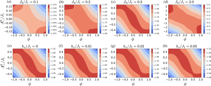
Figure 6: (a-d) The functional $\mathcal{L}_{\text{eff}}(\phi,A^{0}_{-})$ of Eq. (39) plotted in units of $J_{1}$ for different values of $J_{2}/J_{1}$, $h_{z}=0$. (e-h) The effect of the $\mathcal{P}$ breaking term $H_{z}$ on the functional $\mathcal{L}(\phi,A^{0}_{-})$ for a fixed value $J_{2}/J_{1}=0.3$. We can see that one of the non-trivial minima shifts in energy with respect to another one, explicitly breaking the symmetry between two degenerate solution from the $h_{z}=0$ case.

III.2 Effect of the external magnetic field $h_{z}$

We consider the effect of adding an external magnetic field $h_{z}$ to the mean-field solution. In the expression of the fermionic single-particle spectrum this term appears as a Semenoff mass term Semenoff (1984). By doing the numerical minimization, we see that the effect of this perturbation consists in breaking the symmetry between two non-trivial solutions in the regime $0.2\lesssim J_{2}/J_{1}\lesssim 0.36$. This effect is presented in Fig. 6.

IV Exact diagonalization: Classical phases of the frustrated spin-1/2 $XY$ model

In order to determine the phase boundaries of the frustrated spin-1/2 $XY$ model, we calculate the fidelity metric $g$ Zanardi and Paunković (2006); Gu (2010); Varney et al. (2010). The result of this calculation on the lattice of $4\times 3$ unit cells is shown in Fig. 7.

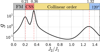
Figure 7: ED calculation of the fidelity metric $g$ on a lattice of $4\times 3$ unit cells for hard-core bosons at filling $1/2$ ($S^{z}_{\text{Tot}}=0$).

Classical phases are studied by looking at the correlation functions $\Braket{S_{\bm{r}_{i}}^{\mu}S_{\bm{r}_{j}}^{\nu}}$ and the related coplanar structure factor

$$S_{\textrm{Spiral}}\left(\bm{q}\right)=2\sum\limits_{i,j\in A}e^{i\bm{q}\cdot\left(\bm{r}_{i}-\bm{r}_{j}\right)}\braket{S^{x}_{\bm{r}_{i}}S^{x}_{\bm{r}_{j}}}\;.$$ (41)

The result of such analysis is presented in Fig. 8.

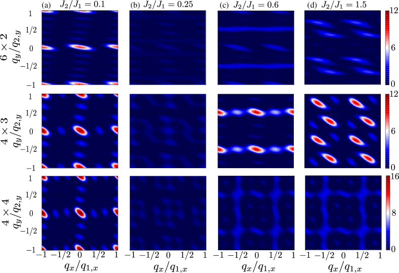
Figure 8: ED calculation of the static structure factor $S_{\textrm{Spiral}}\left(\bm{q}\right)$ at 4 typical points in 4 phases (different rows) on various lattices (different lines) for hard-core bosons at filling $1/2$ ($S^{z}_{\text{Tot}}=0$). Vectors $\bm{q}_{1}$ and $\bm{q}_{2}$ are defined as in Fig. 1(a). (a) In the FM phase ($J_{2}/J_{1}=0.1$ row) the structure factor is piked at $\bm{q}=\bm{\Gamma}$. (b) The systems seems to be disordered in the $xy$ plane in the intermediate frustration regime ($J_{2}/J_{1}=0.25$ row). (c) We observe a formation of the collinear order for $J_{2}/J_{1}=0.6$. We notice however the significant difference of the result on the lattice $4\times 3$. This is explained by the fact that this lattice does not contain all the $\bm{M}$ points in the reciprocal space. (d) In the case $J_{2}/J_{1}=1.5$ the system forms a $120^{\circ}$ order. We notice that similarly to the previous case the lattice $4\times 4$ does not contain Dirac points $\bm{K}$ in the reciprocal space, that results in the impossibility to recover correctly the $120^{\circ}$ phase: two rightmost figures in the bottom line do not differ almost at all.