Optical/Near-IR spatially resolved study of the H II galaxy Tol 02.††thanks: Based on observations obtained at the Southern Astrophysical Research (SOAR) telescope, which is a joint project of the Ministério da Ciência, Tecnologia, e Inovação (MCTI) da República Federativa do Brasil, the U.S. National Optical Astronomy Observatory (NOAO), the University of North Carolina at Chapel Hill (UNC), and Michigan State University (MSU).
Abstract
The main goal of this study is to characterise the stellar populations in very low metallicity galaxies. We have obtained broad U, B, R, I, J, H, K, intermediate Strömgren y and narrow and deep images of the Wolf-Rayet, Blue Compact Dwarf, H II galaxy Tol 02. We have analysed the low surface brightness component, the stellar cluster complexes and the H II regions. The stellar populations in the galaxy have been characterised by comparing the observed broad band colours with those of single stellar population models. The main results are consistent with Tol 02 being formed by a 1.5 Gyr old disk component at the centre of which a group of 8 massive () stellar cluster clumps is located. Six of these clumps are 10 Myr old and their near infrared colours suggest that their light is dominated by Red Supergiant stars, the other two are young Wolf-Rayet cluster candidates of ages 3 and 5 Myr respectively. 12 H II regions in the star-forming region of the galaxy are also identified. These are immersed in a diffuse and emission that spreads towards the North and South covering the old stellar disk. Our spatial-temporal analysis shows that star formation is more likely stochastic and simultaneous within short time scales. The mismatch between observations and models cannot be attributed alone to a mistreat of the RSG phase and still needs to be further investigated.
keywords:
galaxies: star formation - galaxies: star clusters: general - ISM: H II regions - galaxies: photometry - stars: supergiant1 INTRODUCTION
One of the greatest challenges in astronomy is the comprehension of the star formation process that took place inside the very first galaxies formed in the Universe. The key aspects to understand this process are its efficiency to form massive clusters ( ), stellar mass and stellar density of the newly formed star clusters (Adamo et al., 2010; Martín-Manjón et al., 2012; Brennan et al., 2016; Greis et al., 2016). An indirect manner to learn about these primordial star clusters is through the analysis of the star clusters formed in H II galaxies. Although H II galaxies are not necessarily recently formed galaxies, the fact that they are of low metallicity and high gas content implies that they represent relatively unevolved galaxies, probably the low z counterpart of the equally unevolved high z galaxies. This is why a deep understanding of the star formation history of H II galaxies is essential to address the star-formation process in the first formed galaxies (Telles & Terlevich, 1997; Terlevich et al., 2004; Lagos et al., 2011; Martín-Manjón et al., 2012).
H II galaxies were first identified by -and named after- their optical spectrum, which is characterised by a weak stellar continuum dominated by strong emission lines and resembles the optical spectrum of H II regions (Sargent & Searle, 1970; Terlevich et al., 1991). Due to their spectroscopic features -high and low metal content- it was believed that they were the youngest galaxies in the Universe producing their first generation of stars, until deep infrared imaging unveiled their old stellar population with low surface brightness (Thuan, 1983; Cairós et al., 2003; Muñoz-Mateos et al., 2009). Although they do have an older stellar component responsible for their non-zero metallicity, H II galaxies remain as the most unevolved galaxies in the near Universe.
Most H II galaxies do not have an identified companion (Telles & Terlevich, 1995) although in recent years, low surface brightness companions have been found around BCD, starburst, star forming dwarfs and even some objects classified as H II galaxies (Rich et al., 2012; Lelli et al., 2014; Ashley et al., 2017). The morphology of H II galaxies is varied -ranging from spiral to Blue Compact Dwarf (BCD)- and their star-forming regions are frequently composed by multiple knots (Telles & Terlevich, 1997; Méndez & Esteban, 2000; Lagos et al., 2011).
Tol 02 (also known as Tol 0957-278, ESO 435-IG 020, AM 0957-275, PGC 028863, 2MASX J09592122-2808000, NVSS J095921-280805) was first identified as an H II galaxy due to its intense emission lines (Smith et al., 1976; Terlevich et al., 1991; Kehrig et al., 2004). It is an isolated galaxy located in the southern sky (R.A = 095921.21, Dec. = -280800.3, J2000) at a redshift z=0.003 (Distance Mpc) with an angular diameter of arcsec. A bright star-forming region with high intensity emission lines and low gaseous metallicity (Vacca & Conti, 1992; Mayya, 1994; Buckalew et al., 2005; Engelbracht et al., 2008) lies at its centre. This galaxy has also been classified as a BCD galaxy because of its low B band magnitude (Kunth et al., 1988; Doublier et al., 1999; Gil de Paz et al., 2003) and as a Wolf-Rayet galaxy candidate due to the broad emission line observed in its integrated spectra (Kunth & Joubert, 1985; Schaerer et al., 1999).
Previous research on Tol 02 has focused on the integrated spectrum of the galaxy (Smith et al., 1976; Kunth & Joubert, 1985; Terlevich et al., 1991; Schaerer et al., 1999; Kehrig et al., 2004). These have concluded that the galaxy is composed of multiple stellar populations, in which the dominance of extremely young - Myrs old- and Red Super Giant (RSG) stars are eminent, while the older stellar populations with ages greater than Myr is modest (Raimann et al., 2000; Westera et al., 2004). Few photometric studies have been performed in this galaxy, and they have focused in the decomposition of the galaxy into a disk -or host galaxy formed by the old stellar populations- and a star-forming region. A previous characterisation of the galaxy H II regions was performed by Méndez & Esteban (2000), where they did not identify the stellar populations in the continuum images.
The characteristics of Tol 02 described before -isolated H II galaxy, BCD classification, projected size > 30 arcsec-, as well as the previous results found on the galaxy -extremely low brightness old stellar population, possibility of finding Wolf-Rayet and RSG stars- made us realise that this galaxy was an excellent target to analyse the star formation process. The main goal of this study is to characterise the photometric properties, ages and masses of the stellar populations in the galaxy by identifying its structural components.
In Section 2, we describe the observations and data reduction procedures. In Section 3, we compare our results on the galaxy optical broad and narrow band integrated photometry with values reported in the literature. In Section 4, we analyse the photometry of the galaxy low surface brightness component, the star-forming region, and the identified stellar cluster complexes and H II regions. In Section 5, we describe the procedure used to characterise the age, mass and extinction of the stellar populations. In Section 6, we discuss the photometric and modelled properties of the stellar populations derived and our conclusions on the stellar populations that dominate the galaxy photometry.
2 OBSERVATIONS, DATA REDUCTION AND CALIBRATION
The data were obtained at SOAR, the 4.1m telescope situated in Cerro Pachón, Chile, in service mode. Images in optical and near infrared bands were taken and the instrumentation used is described below.
Optical U, B, R and I broad-, y Strömgren intermediate- and and narrow-band images were obtained on February and May of 2010 using SOAR Optical Imager (SOI), with a characteristic seeing of 0.8 arcsec. SOI is a mini-mosaic comprised of two CCDs of 2048x4096 pixels each and mounted with their long sides parallel and spaced 102 pixels apart. Each CCD is read by two different amplifiers, resulting in a mosaic image formed by four data frames. The sky area covered by this image is arcmin2 (with a central gap of 7.8 arcsec wide) and a 0.1534 arcsec pixel-1 plate scale in the 2x2 binned mode.
NIR broad-band J, H and K images were taken on March 2012 with Spartan, SOAR infrared camera. Spartan is a mosaic formed by four HAWAII-2 detectors (2048x2048 ). The wide field mode was used, covering a sky area of arcmin2 with a gap between detectors of 0.47 arcmin, and a plate scale of 0.07 arcsec pixel-1. The galaxy was centred on detector 3 (Tol 02 major diameter is only 0.8 arcmin), since this is the one with the best response. The other detectors were not used. The dithering pattern of the images followed a six points rectangular path. Each consecutive image was taken with a 5 arcseconds displacement in either right ascension or declination.
The observing log is presented in Table 1, where column 1 is the date of observation, column 2 the filter, column 3 the total exposure time in seconds (as a combination of several exposures), column 4 the mean airmass of the observations and column 5 the seeing of the image in arcseconds. The properties of the optical and NIR filters111http://www.ctio.noao.edu/soar/content/filters-available-soar are given in Table 2. Column 1 is the filter name, column 2 the central wavelength in Ångstroms, column 3 the FWHM in Ångstroms and column 4 the relative transmission at the central wavelength.
| Date | Filter | Exp. Time | Airmass | Seeing |
|---|---|---|---|---|
| (s) | (″) | |||
| 11-Feb-2010 | U | 1200 | 1.08 | 0.8 |
| 11-Feb-2010 | B | 900 | 1.05 | 0.8 |
| 11-Feb-2010 | R | 900 | 1.03 | 0.6 |
| 11-Feb-2010 | I | 900 | 1.02 | 0.6 |
| 09-May-2010 | 1800 | 1.17 | 1.0 | |
| 09-May-2010 | [OIII] | 1800 | 1.10 | 1.0 |
| 11-Feb-2010 | y Strömgren | 600 | 1.01 | 0.7 |
| 3-Mar-2012 | J | 1700 | 1.01 | 0.9 |
| 3-Mar-2012 | H | 2500 | 1.08 | 0.7 |
| 3,4-Mar-2012 | K | 3570 | 1.07 | 0.7 |
| Filter | FWHM | ||
|---|---|---|---|
| U (SOI) | 3624 | 784 | 60.68 |
| B (SOI) | 4326 | 1269 | 73.76 |
| R (SOI) | 6289 | 1922 | 76.97 |
| I (SOI) | 8665 | 3914 | 95.28 |
| H (CTIO 660075-4) | 6600 | 67 | 84.77 |
| (CTIO 5019) | 5027 | 50 | 79.48 |
| y Strömgren | 5478 | 244 | 70.83 |
| J | 1.25 | 0.16 | 84.77 |
| H | 1.64 | 0.29 | 95.41 |
| K | 2.20 | 0.34 | 87.27 |
2.1 Optical data
Standard image reduction was performed individually to each of the optical frames using IRAF222IRAF (Image Reduction and Analysis Facility) is distributed by the National Optical Astronomy Observatories, which are operated by the Association of Universities for Research in Astronomy (AURA), Inc., under cooperative agreement with the National Science Foundation.. This includes bias subtraction, flat-fielding and cosmic-ray elimination by combining multiple exposures. Astrometric solution was applied using the tasks ccxymatch and ccsetwcs from the images package. Each galaxy image was formed by grouping the four reduced frames using wregister and imcombine. Once the complete image was obtained the median sky value was subtracted. The sky value of this combined image was calculated as the median of the Gaussian that best fitted the image counts distribution. We have degraded all images into the same spatial resolution given by the image with the worst seeing (which turned out to be the image), calculated using the field stars full width at half maximum (FWHM). The optical images final resolution is 1 arcsec.
2.2 NIR data
The NIR reduction steps are based on Loh et al. (2011) and Mayya et al. (2005). We used IRAF tasks to perform the image processing. The process included correction for bad pixels, sky subtraction in order to achieve zero mean sky value, field stars subtraction, sky flat correction of pixel to pixel CCD response variation and astrometric alignment of the images.
2.3 Flux calibration
The images were calibrated using standard methods described in Appendix A. Two spectrophotometric standard stars from Hamuy et al. (1992) were used to calibrate the optical images (both broad and narrow bands). The NIR images were calibrated using four faint NIR standard stars from Persson et al. (1998).
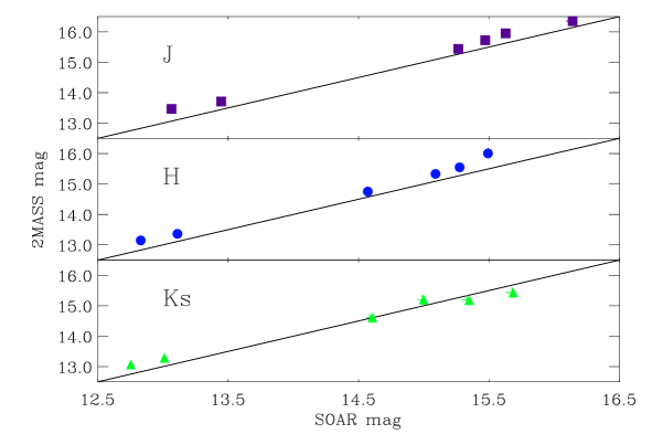
We have compared the magnitudes of field stars identified in both SOAR and 2MASS images (Figure 1 and Table 3). Unfortunately, most of the stars are dimmer than the 2MASS average limits, J = 15.8 mag, H = 15.1 mag and Ks = 14.3 mag (Skrutskie et al., 2006), although all of them were classified as having a SNR > 10 thus good photometry333The 2MASS user’s guide indicates that the point source photometric sensitivity varies from frame to frame, therefore the SNR = 10 level is usually achieved at fainter magnitudes than the ones imposed as the survey limits, as is the case for the image frames of Tol 02 (http://www.ipac.caltech.edu/2mass/releases/allsky/doc/sec2_2.html). . Table 3 shows that our J and H values are magnitudes lower than the ones calculated by 2MASS while a much better agreement is found in the K band. A possible cause for this systematic difference could be different filter response between the 2MASS and SOAR systems.
| Filter | Mean | Median |
|---|---|---|
| (mag) | (mag) | |
| J | ||
| H | ||
| K |
2.4 Emission line images
Emission line images were obtained after subtracting the continuum contribution to the narrow band filter images. The amount of continuum in the narrow band images was estimated by comparing the field stars flux in narrow, broad and intermediate band images. This procedure is based on the premise that the field stars flux in the narrow band images is none other than the continuum flux contribution to the image, since stars usually do not present emission lines. Therefore, the field stars broad and intermediate band flux () was scaled by a constant to match the flux of the stars in the narrow band image (). The scaled R and y Strömgren images were used to estimate the continuum flux in the and images respectively.
The emission line is one of the brightest lines in the optical spectrum and the most important contribution of nebular emission inside the R band image. For this reason we have subtracted the pure emission image from the R band image before performing any analysis. All the results regarding the R band refer to this subtracted R band image.
3 PHOTOMETRY
3.1 Broad band
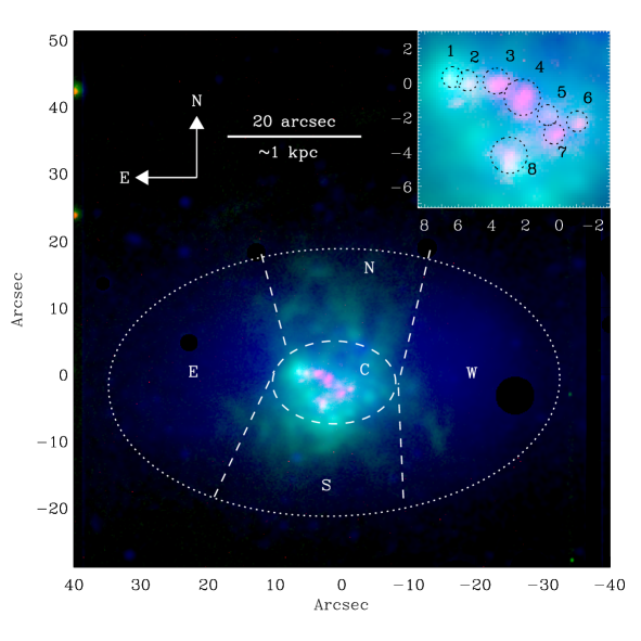
A composite optical-NIR image is shown in Figure 2. It is formed by the NIR J band image in red, optical B band image in blue and emission image in green. The figure shows in blue the B band surface brightness decreasing from the centre outwards, forming an elongated body. In this figure, the 25 B magnitude isophote is fitted by an ellipse with a major axis arcsec and a minor axis B = 40 arcsec ( kpc and kpc at the adopted distance). The centre of this ellipse will be referred to as the (photometric) centre of the galaxy (R.A. 09h59m21.00s, Dec. -28d07m59.40s).
The optical magnitudes (U, B, R and I) of the galaxy were obtained by integrating the light collected inside the B 25 magnitude isophote. The absolute magnitudes and luminosities of both broad and narrow band filters (assuming a distance444Calculated assuming a uniform Hubble flow with and 826 (Mould et al., 2000) for the recession velocity of the object. of 11 Mpc) were corrected for galactic extinction using Cardelli et al. (1989) equations and a colour excess of E(B-V) = 0.094 mag obtained from the NASA/IPAC Extragalactic Database (NED). No internal extinction correction was applied. Our results -with and without galactic extinction correction- are shown in Table 4 together with those from Doublier et al. (1999); Méndez & Esteban (2000); Gil de Paz et al. (2003), hereinafter DO99, ME00 and GI03, respectively. The table shows a spread of mag, our B and R values being the highest ones. Our B band magnitude (corrected from galactic extinction) is mag higher than the B band magnitudes in DO99 and GI03. This discrepancy is comparable with the magnitude difference found between GI03 and DO99 for the 23 galaxies they have in common. Our R band value differs 0.02 and -0.28 magnitudes from GI00 and DO99, respectively. The difference between our and DO99 values can be accounted for by the different methods used to calculate the integrated magnitude of the galaxy. DO99 used a modelled light profile from the galaxy. Both GI03 and us obtained the integrated magnitudes of the galaxy by using aperture photometry instead. Therefore, we attribute the discrepancy to the use of different methods to remove field stars and nearby galaxies.
The U band magnitude for this galaxy has been published in ME00. Our U and B extinction corrected values are 0.52 mag greater. This difference is primarily due to the different extinction correction performed, since ME00 considered internal extinction, using the Balmer decrement reported by Vacca & Conti (1992) and Whitford (1958) extinction law. Our extinction corrected colours are in agreement with those from DO99, GI03 ( mag) and ME00 ( mag). We did not find in the literature an I band integrated magnitude value for this galaxy.
| U | B | R | I | Reference |
|---|---|---|---|---|
| 14.04 | 14.59 | 13.57 | 13.20 | This work (Observed) |
| 13.59 | 14.20 | 13.32 | 13.05 | This work (E(B-V) corrected) |
| 14.08 | 13.04 | DO99 | ||
| 13.07 | 13.68 | ME00 | ||
| 14.06 | 13.34 | GI03 |
| ID | |||||
|---|---|---|---|---|---|
| Galaxy | 1250 | ||||
| North | 515 | ||||
| West | 674 | ||||
| South | 531 | ||||
| East | 635 | ||||
| Centre | 395 |
The galaxy was divided into five zones: North, West, South, East and Centre. The limits were imposed by the U-B colour map morphology of the galaxy and are indicated in Figure 2. The B absolute magnitude and the optical colours of the integrated galaxy and its five zones are presented in Table 5. Column 1 is the zone’s name, column 2 is the B band absolute magnitude and columns 3 to 5 are the U-B, B-R and R-I colours, respectively. The uncertainties of the parameters presented in the table are lower than except for U-B with a uncertainty for all zones. The Centre zone is delimited by the 22 B mag isophote, has an elliptical shape with a major axis of arcsecs ( kpc) and a blue U-B = -0.7 mag colour. The North and South zones also show blue colours with mag and mag, respectively. Together, these three zones form a blue strip that separates the East and West zones, which have redder colours of . The B-R map shows a homogeneous red disk-like structure formed by all the zones but the Centre. A blue () circular structure with a arcsecs radius is observed at the centre of the galaxy, exceeding the Centre zone.
Only discrete sources can be identified in the infrared data due to the insufficient depth. They will be discussed in Section 4.2.1.
3.2 Narrow band
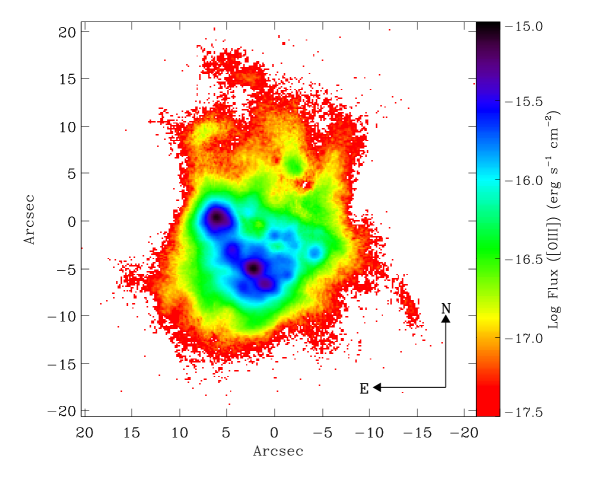
The present star-forming region is delimited by the emission (Figure 2) which is located at the Centre zone of the galaxy and extends towards the North and South zones. Figure 3 shows the emission map, which shows a similar spatial distribution as the emission, albeit on a different flux scale. Structures as faint as (with more than confidence) are identified in both and images.
The integrated flux, luminosity (corrected by galactic extinction and the contribution of the [NII] lines and equivalent width of both and of the star-forming region (SF) are given in Table 6. The [NII] contribution to the flux was removed using the values obtained from Kehrig et al. (2004) long slit spectrophotometry and and assuming that these values are constant across the starburst. The equivalent widths were calculated by using the nebular and continuum light within the aperture.
| Reference | |||
| This work | |||
| ME00 | |||
| GI03 | |||
| Reference | |||
| This work |
integrated flux on Tol 02 had been previously analysed in ME00 and GI03. As in GI03 we use the R band image to determine the continuum contribution to the image, while a narrow band filter adjacent to the filter central wavelength is used in ME00. The three studies show a similar luminosity; ours is 4% and 10% higher than those of ME00 and GI03, respectively555The luminosity has been corrected to the same (11 Mpc) adopted distance.. On the other hand, the from ME00 is times higher than those in GI03 and this work. This difference is believed to arise from the sensitivity of the to the continuum subtraction.
4 ANALYSIS
4.1 Extended Low Surface Brightness Component
Most blue compact dwarf galaxies consist of two main stellar structures (Kunth & Östlin (2000); Papaderos et al. (1996); Telles & Terlevich (1997) and references therein): a young star-forming region and an older low surface brightness component (LSBC) which pervades the complete body of the galaxy. This LSBC can only be appreciated outside the area covered by the emission, and its light dominates the galaxy surface brightness profiles (SBP) faint levels ( mag arcsec-2). In the previous sections we described the photometric properties of the star-forming regions and of the individual star clusters. Here we use the optical broad band images to analyse the LSBC.
4.1.1 Surface Brightness Profiles
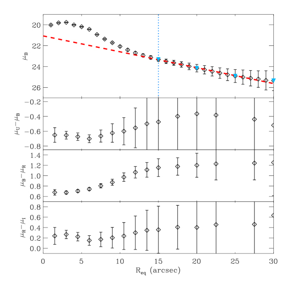
There are several methods to obtain SBP (Bergvall et al., 1999; Papaderos et al., 1996; Cairós et al., 2001; Micheva et al., 2013). Most of them represent the galaxy flux through a spherically-symmetric distribution , where is the photometric radius corresponding to the surface brightness level . Apart from being simple in performance and visualisation, a spherically-symmetric distribution allows analysis of the colour profiles change as a function of distance to the centre.
Therefore we use concentric ellipses with fixed axis ratio to determine the surface brightness level at an equivalent radius , where and are the ellipse semi-axes. The equivalent radius ranges from to arcsec with fixed steps of arcsec. The concentric ellipses centre and axis ratio () was set by the ellipse that best fitted the 25 mag isophote in the B band image. The SBPs were computed using an increment arcsec.
The B SBP at the top panel of Figure 4 shows a clear exponential decay at equivalent radii greater than 15 arcsec. The U, R and I SBPs (not shown) also describe an exponential decay, similar in shape to the one in B but shifted in magnitude. Even if the exponential disc should be better sampled in the I band, the low intensity values uncertainties are considerably increased by a fringing problem.
The U-B, B-R and R-I colour profiles are also shown in Figure 4, uncertainties were determined as: . The colours (albeit with large errors) are redder from the centre outwards, as previously noticed by Kunth et al. (1988) and DO99. We cannot determine whether the U-B colour profile really becomes bluer from the arcsec outwards or if that is just an artefact of the large uncertainties present.
4.1.2 LSBC exponential disc model
As already mentioned, the exponential decay observed in the SBP has been found previously by Kunth et al. (1988) and DO99. We fitted the observed SBP for each band with an exponential disc model, , assuming that . To avoid contamination from the nebular emission due to recent star formation, the model was fitted to the profiles in the radial range where the contamination is negligible ( to arcsec).
Table 7 shows the parameters for each fitting; column 1 is the filter name, column 2 is the surface brightness magnitude in units of at arcsec, column 3 is the scale length in parsecs and column 4 the I band surface brightness magnitude in at arcsec scaled to match the SBP of the other filters at arcsec. The exponential disc model that best fit the B SBP is shown in Figure 4 as a red-dashed line; the blue dotted vertical line indicates the innermost equivalent radius at which the fitting was performed ( arcsec).
| Filter | |||
|---|---|---|---|
| (pc) | |||
| U | |||
| B | |||
| R | |||
| I |
The modelled disc parameters, individually determined for each band, were used to create images of the LSBC in all the optical bands. We also used the I band fitted disc model (scaled to match the SBP of the other filters at the radius arcsec) to create images of the disc population as represented by the I band dominant stellar population (). In both cases we used two elliptical apertures to measure the photometry in the modelled LSBC and , as well as in the data. The first elliptical aperture encloses the star-forming area using an equivalent radius of arcsec. The second represents the galaxy 25 B mag isophote with arcsec.
| Aperture | Object | ||||
|---|---|---|---|---|---|
| Star-forming | |||||
| Star-forming | SF | ||||
| Star-forming | |||||
| 25 B mag | LSBC | ||||
| 25 B mag | |||||
| 25 B mag | Galaxy |
With the calculated photometry we have analysed the disc stellar population (LSBC and ) contribution to the star-forming area and overall galaxy light emission. We found that although the star-forming area aperture accounts for 99% of the optical light observed in the galaxy, the disc stellar population light contribution is not negligible. Half of the light observed inside the star-forming area aperture is emitted by the disc stellar population (LSBC = 54%, % ). The contribution of the disc population to the total U band flux of the whole galaxy is higher than 30%, independently of the model used (LSBC = 43% and %), and 68% for the I band.
This important flux contribution from the disc stellar population affects both the colours of the galaxy integrated photometry and of the galaxy star-forming area. The colours of the two apertures: star-forming area and galaxy are presented in Table 8, where column 2 is the absolute B magnitude and columns 3 to 5 are the U-B, B-R and R-I colours respectively. For the galaxy aperture we tabulate the observed colours of the galaxy as well as those for the modelled disc populations (LSBC and ). As well, for the star-forming region we tabulate the observed values () and the values after subtracting the disc stellar population contribution (SF and ). The net effect of the disc population is a reddening of the star-forming area colours by , and magnitudes, more pronounced at the U-B colour for the LSBC than for the model, while for R-I is the other way round. We find that by identifying the light contribution of the disc population to the galaxy not only we can characterise the old stellar component, but it also helps to constrain the colours of the stellar populations in the star-forming region.
4.2 Star-forming region
To describe the nebular properties of the galaxy in two dimensions, the narrow band images were divided in square cells of 1.5 arcseconds side and the light within each cell was integrated. Only those cells with value above were considered for the photometry. The cells size was chosen to be greater than the seeing ( arcsec). Given the physical size of the cells ( pc at the adopted distance of the galaxy), each cell might contain one H II region, although most H II regions are larger in size (H II regions sizes can reach up to a few hundred parsecs).
The and [OIII] equivalent width (EW) maps were created by using the narrow band emission line and continuum images (Section 2.4). Both maps show a linear shape structure with high equivalent width values ( Å) that corresponds to the position of the bright nebular emission peaks observed in Figure 3.
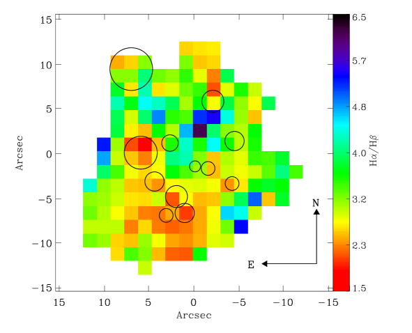
The dust extinction distribution in the star-forming region of the galaxy is described by the map (Figure 5), which was created using an emission line image from Lagos et al. (2007). The map suggests that the cells with the lowest extinction values are located on top and to the South of the chain of H II regions and the cells with the highest extinction values are grouped North-West. The theoretical value of an extinction free ISM is 2.86 (Osterbrock & Ferland, 2006), and it increases exponentially with the amount of dust. The map encompass values from 1.5 to 6.5. Although the calculated value is lower than 2.86 for % of the cells, this percentage reduces to 16% when the uncertainties are taken into consideration (). Still, the extremely low values might be a product of a calibration mismatch between images, originated by a shift in the absolute photometry due to differences in atmospheric conditions, calibration standard stars, image continuum subtraction, etc. If there was indeed a mismatch in the calibration between the different programmes when H and H were obtained, such as it would affect all the cells. However, when combined with our cutoff such a mismatch would produce an underestimate of the flux of (the weakest line) in the fainter regions which in turn would increase the Balmer decrement.
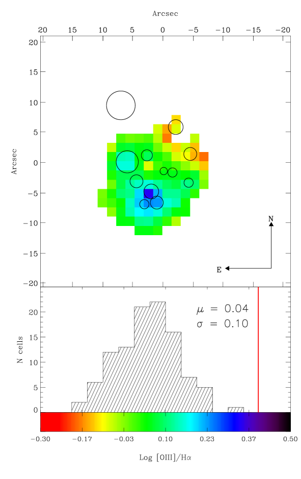
The ionisation hardness map, obtained through the and images ratio, identify the area where the ionising photons are concentrated. These two emission lines are close enough in wavelength for the ratio to be insensitive to extinction. The ratio can be assumed as an extinction dependent analogous of the ratio. Both ratios map display the same morphology, indicating that the extinction is not severe and quite uniform. The map is shown in Figure 6. A low excitation area is observed towards the NW, suggesting that the mean energy of the ionising photons produced by the stellar sources in this area is lower than in the rest of the map. In emission line maps, this area is attributed to what seems to be diffuse emission. The highest values of ionisation hardness are observed at the position of the southernmost nebular peak.
The distribution of is presented at the bottom of Figure 6. We have used the intensity of the emission lines from the star-forming region (from Terlevich et al., 1991), to calculate the nebular photoionisation threshold line (Kewley et al., 2001). This was calculated assuming that the interstellar medium in the galaxy is extinction-free () and that its [NII] to ratio is uniform, with an estimated value of . We notice that all the value of the cells lie to the left of the threshold line value, with a mean value of , thus indicating that the interstellar medium is indeed being photoionised by young massive stars.
4.2.1 Star Cluster Complexes
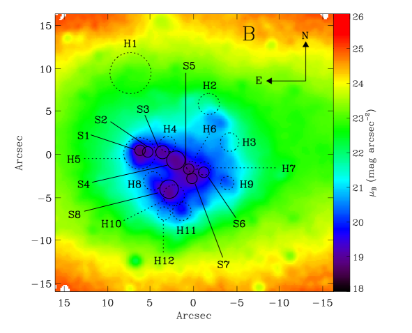
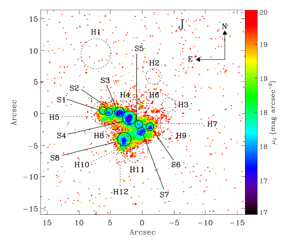
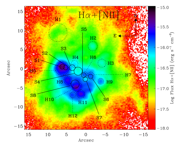
A relevant feature seen in Figure 2 is the eight bright knots at the Centre zone of the galaxy in both NIR and optical images, which can be clearly identified by eye (see the insert of Figure 2). These stellar knots are aligned in a “>” shape structure. Although this chain of knots has been previously identified in optical bands (Doublier et al., 1999), this is the first time that their photometry is analysed. All of the knots are outlined by circular shapes with radii in the range of 30 to 60 pc. Since typical star cluster sizes vary from 1 to 20 pc, each of these knots might contain more than one star cluster. Therefore, these knots are interpreted as star cluster complexes (SCCs). For a given SCC, the aperture size depends on the seeing, the curve of growth of its light profile and its proximity to the nearest neighbour. As a first approximation, the SCC centre is set as the position of the local maximum in the B band surface brightness map. The curve of growth rarely decreases due to the bright background and proximity to neighbours. Therefore, we analyse the surface brightness isocontours to delimit the knots using a uniform increment of . The isocontours enclosing each knot centre are fitted by circles. The adopted radius for each object is that of the circle fitted to the outermost isocontour without overlapping with another object, unless the overlapping was needed in order to reach a radius of at least the FWHM size. Figure 7 presents the SCCs apertures over the optical B, NIR J and nebular maps.
To calculate their photometry, the local background emission which was determined as the median value of the light within a concentric ring around the aperture (Adamo et al., 2010; Lagos et al., 2011; Álvarez-Álvarez et al., 2015) was subtracted from the light within the aperture. To avoid overestimating the level of the local background due to the neighbouring SCC, only pixels that are not shared with other SCC regions were used to estimate the local background emission. The SCCs position, aperture radius and optical and NIR photometry are presented in Table 9, where column 1 is the SCC ID number, columns 2 and 3 are the right ascension and declination distance from the centre in arcsecs respectively, column 4 is the radius in parsecs of a circle that has the same area as the region, column 5 and 6 are the B and J band absolute magnitudes and columns 7 to 11 are the U-B, B-R, R-I, I-J and J-H colours, respectively. The K band photometry is not reported because for all of the SCCs we could not determine accurately the local background level, since up to % of the pixels inside the background aperture annulus had flux values below level.
| SCC | ||||||||||
|---|---|---|---|---|---|---|---|---|---|---|
| 1 | -6.37 | 0.32 | 33 | |||||||
| 2 | -5.48 | 0.13 | 33 | |||||||
| 3 | -3.76 | 0.10 | 41 | |||||||
| 4 | -2.21 | -0.84 | 58 | |||||||
| 5 | -0.71 | -1.88 | 33 | |||||||
| 6 | 1.04 | -2.24 | 33 | |||||||
| 7 | -0.33 | -2.96 | 33 | |||||||
| 8 | -2.99 | -4.21 | 58 |
SCCs #1 and #2 are the bluest and are located at the eastern tip of the chain of SCCs. These SCCs have a radius of pc and overlap each other. It is worth noticing that even though SCCs #1 and #2 have similar optical colours, SCC #1 has different NIR colours than SCC #2 by mag and mag. These differences in colour will be essential when analysing dominant stellar population of the SCCs, as discussed in Section 5.2.3.
Another interesting SCC is #4, which is located in the centre of the upper line of knots. It is the brightest knot in both optical and NIR bands () and its colours are similar to the mean values of the knots. The U-B colour of the complexes seems to become redder towards the west, although no clear colour gradient is observed. As for the other colours (B-R, R-I, I-J and J-H), the SCCs do not show any tendency or pattern at all. The SCCs optical broad band photometry uncertainties are typically 5%, the highest value is 12% and corresponds to SCC # 6. The NIR bands uncertainties are higher, around 14% for the magnitudes and up to 18% for the NIR colour of SCC #5.
4.2.2 H II regions
Identifying and setting boundaries for H II regions is not an easy task (see, e.g. Álvarez-Álvarez et al., 2015). images show H II regions as bright spheroids enclosed by a diffuse and irregular extended emission whose boundaries might overlap with those of a neighbouring H II region. Even sophisticated software packages designed to find local maxima and minima in images, such as SExtractor (Bertin & Arnouts, 1996) and FOCAS (Valdes, 1982), are likely to fail since they tend to confuse H II regions with diffuse emission and detect elongated objects which might be thinner than the image resolution.
On the contrary, the identification and border delimitation of H II regions through careful eye inspection has been a widely used method and has proven to be effective albeit time consuming. Thus, to identify and delimit the H II regions in the image of this galaxy, we have chosen this method. We were able to identify twelve H II regions. Following the same procedure as for the SCCs, the objects were identified by eye and the position of the maximum flux in each knot was set as first approximation of the object centre. The curve of growth and the flux increment for each object was calculated. If at some radius the flux increment began decreasing, then the radii at the minimum flux value was set as the maximum radii for the object. Otherwise the maximum radius was set free. The isocontours of the images were drawn using uniform flux increments Å-1 and a circle was fitted to the isophotes until it reached the maximum radius value set by the curve of growth or when the isophote starts engulfing other object. All H II regions in the galaxy are located at the Centre and North zones. The circular apertures used to calculate the photometry were shown with dotted lines in Figure 7. The five brightest H II regions (5, 8, 10, 11 and 12) correspond to the emission peaks observed in the and maps. They are aligned from Centre to South and show a shift from the position of the SCCs (dotted lines). Only the H II region #5 engulfs two SCCs ( and ).
The photometry of the H II regions was calculated with the same method as for the SCCs. Table 10 presents the narrow band photometry results of the H II regions. Column 1 is the H II region ID, columns 2 and 3 are the right ascension and declination distance from the centre in arcsecs respectively, column 4 is the H II region radius in parsecs, columns 5 and 6 are the observed and flux in , columns 7 and 8 are the extinction corrected luminosity in and columns 9 and 10 are the equivalent widths in Å. For 6 H II regions we could also measure the optical broad band photometry, which is presented in Table 11 where column 1 is the H II region ID, column 2 the B band absolute magnitude and columns 3 to 5 are the U-B, B-R and R-I colours, respectively.
| H II | |||||||||
|---|---|---|---|---|---|---|---|---|---|
| 1 | -7.48 | 9.31 | 128 | ||||||
| 2 | 1.63 | 5.72 | 66 | ||||||
| 3 | 4.05 | 1.27 | 58 | - | - | - | - | ||
| 4 | -3.16 | 1.04 | 50 | ||||||
| 5 | -6.42 | -0.04 | 99 | ||||||
| 6 | -0.36 | -1.57 | 33 | - | - | ||||
| 7 | 1.10 | -1.80 | 41 | ||||||
| 8 | -4.89 | -3.26 | 57 | ||||||
| 9 | 3.78 | -3.49 | 41 | ||||||
| 10 | -2.43 | -4.95 | 66 | ||||||
| 11 | -1.51 | -6.79 | 57 | ||||||
| 12 | -3.58 | -7.05 | 41 |
| H II | U-B | B-R | R-I | |
|---|---|---|---|---|
| 1 | ||||
| 5 | ||||
| 7 | ||||
| 9 | ||||
| 10 | ||||
| 11 |
Important parameters of the H II regions derived from the narrow band luminosities are the , the star formation rate (SFR), the equivalent number of O7V ionising stars () and the Strömgren radius (). These are described in the following paragraphs and their values are presented in Table 12, where column 1 is the ID of the H II region, column 2 is the ratio in logarithm, column 3 is the SFR per surface area () in units of , column 4 is the number of main sequence ionising stars and column 5 is the Strömgren radius in parsecs. The SFR is an indicator of the amount of gas transformed into stars at a time interval. We derived it using Calzetti’s rendition (Calzetti et al., 2010) , which assumes a Salpeter IMF with stellar mass range . Since H II regions are short-lived objects, it is assumed that they formed instantaneously, and the specific SFR per unit area () can be interpreted as an indicator of the surface density of massive stars. The number666This is a lower limit since we are assuming no escaping photons. of massive stars needed to ionise the observed H II emission (assuming no escaping photons) can be described by the luminosity as , where is the ionising photons rate.
Assuming a homogeneous ISM, the Strömgren sphere (Osterbrock & Ferland, 2006) defines the volume in which all of the ionising photons emitted by the ionising stellar source are absorbed and re-emitted by the ISM and where the hydrogen is fully ionised. The Strömgren radius of the identified H II regions is given by , where is the H I recombination coefficient and the electron density of the nebula calculated through the sulphur lines ratio () from Kehrig et al. (2004).
Tol 02 H II regions are all brighter in than in , have a luminosity of , Å and U-B colours bluer than mag. The values of the H II regions range from 0 to 0.5, typical values for H II galaxies (e.g. Kehrig et al., 2004) These authors also obtained the values for the regions #5 and #11 as 0.05 and 0.04, respectively. These values are lower than the ones we found, but are similar to the median value of the cells ( = 0.04, Figure 6). It is worth noticing that the values of the H II regions is greater than the values from the cells of the mesh. The H II regions with the highest values (#10, #11 and #13) are located south and coincide with the highest peak of the map.
The four brightest H II regions (aligned from the centre to the southwest) are the ones with the highest values, and the brightest H II region (#5) is the one with the highest value of all (), two orders of magnitude higher than the median (). As well, H II region #5 can be associated to massive ionising stars, followed by H II region #10 with 23 stars. Only these four H II regions are associated to more than 10 massive stars, while the rest could be photoionised by less than four. These regions are also those for which the difference between the Strömgren and radii is the smallest, albeit the for all of them.
| H II | ||||
|---|---|---|---|---|
| 1 | ||||
| 2 | ||||
| 3 | - | |||
| 4 | ||||
| 5 | ||||
| 6 | ||||
| 7 | ||||
| 8 | ||||
| 9 | ||||
| 10 | ||||
| 11 | ||||
| 12 |
Eight of the H II regions identified in this work were previously studied by ME00 using , U, B and V images taken with the 2.6 m Nordic Optical Telescope (NOT) in La Palma. To identify and analyse the H II regions they used FOCAS, which is a set of programs primarily designed to identify small faint objects and segregate them in stars, galaxies or noise. FOCAS identifies local maxima in images and encloses them using irregular areas built after analysing the image isocontours. Unfortunately, FOCAS is no longer supported by the NOAO-IRAF community, which makes it impossible for the authors to install the package for analysing our images. Therefore, in order to achieve a comparison as similar as possible to ME00, we have recalculated the luminosity values of our identified H II regions by using irregular apertures delineated by the image isocontours. Since the area covered by the H II regions is not shown in ME00, the isocontours used were chosen so that the total luminosity of the H II region resembled the value provided by ME00. The luminosity was subtracted from local background emission and corrected for intrinsic extinction777The intrinsic extinction was estimated using the same approach as ME00 applying Whitford (1958) extinction law and Vacca & Conti (1992) value, assuming the same distance to the galaxy as ME00 for comparison. With this approach, our luminosities are 30% higher than those by ME00, which is not surprising since our images are deeper than theirs. The luminosity difference can also be severely affected by variations in the local background emission subtracted (due to a difference in the H II region shape).
5 STELLAR POPULATIONS CHARACTERISATION
5.1 Spectral Energy Distribution Fitting
The age, mass and extinction values of a specific stellar population can be inferred by comparing its photometric colours with those of synthetic stellar populations (Anders & Fritze-v. Alvensleben, 2003; Adamo et al., 2010; Rodríguez-Merino et al., 2011; Martín-Manjón et al., 2012). PopStar single stellar populations (SSP) models (Mollá et al., 2009) cover an age range from 0.1 Myr to 15 Gyr, metallicities from Z=0.0001 to Z=0.05 and take into consideration the nebular continuum contribution to the stellar spectral energy distribution (SED). The wide age range covered by PopStar models allows to analyse both young and old stellar populations contained in BCD galaxies while the low metallicity models are ideal to study H II galaxies. Therefore, we use a Z=0.004 PopStar model to characterise the stellar populations in Tol 02 since it is the one that best suits the galaxy Z=0.0035 value888Assuming where (Vacca & Conti, 1992).. We followed Rodríguez-Merino et al. (2011) SED fitting method to compare the observed colours with those of the SSP models. The method is described briefly as:
-
1.
Build a set of reddened SSP SEDs. The magnitudes and zero points at a given epoch were calculated by convolving SOAR filters transmission curves with the SED of both the modelled SSP and the star Vega (Pickles, 1998). The magnitudes were calculated at the 106 irregularly sampled PopStar time points that span the age range from Myr to Gyr. These were then reddened using an extinction vector ranging from to mag at magnitudes steps.
-
2.
Obtain SSP uniformly sampled time. The temporal evolution (in logarithmic scale) of the reddened magnitudes was linearly interpolated using a Myr time step, to keep all 106 PopStar original points. The final time vector consists of 1041 uniformly distributed time steps in the range Myr to Gyr.
-
3.
Defining the merit functions. The colours of each object were compared to those of the modelled SSPs using two merit functions. The first one is defined as:
(1) where N is the number of different colours to analyse, and are the modelled and observed colours respectively, and is the object photometric colour uncertainty. The colours used in this first merit function were built using the R band as reference: U-R, B-R, R-I, R-J and R-H. The second merit function relies on the U-B colour potential to differentiate the ages of stellar populations younger than 500 Myr (the U-B colour of a SSP spans 1.3 magnitudes from 0.1 to 500 Myr) and is defined as:
(2) The use of this function strengthen the unicity of the solution. We selected the 50 models associated with the lowest values, and of these kept only those that are within the 10% of the minimum value of .
-
4.
Simulated data sets. We used Monte Carlo simulations to create a set of 5000 fake observations at each of the seven bands. The flux of the fake observations at each of the bands was randomly chosen from a Gaussian distribution with a mean value equal to the observed flux and a sigma value equal to its uncertainty. We used the merit functions to determine the capability of the models to reproduce the colours of the fake observations. For each of the 5000 fake observations we kept the models associated to the lowest and values, and combined them with the model that best fit the object photometry. This gave as a result a collection of various thousands of models related to the photometric values of the object under study.
-
5.
Age and extinction determination. A Gaussian function was fitted to the distribution of ages (in logarithmic scale) and extinction values that best reproduced the object photometric SED. The mean value of the fitted Gaussians are adopted as the and values of the object representative stellar population, and the Gaussian standard deviation is taken as an uncertainty measure of the adopted and values.
-
6.
Age and extinction uncertainties. The uncertainties of the adopted age and extinction values only take into consideration the uncertainties from the photometry. To consider the uncertainty of the fitted age due to the discrete time steps we have added to the age uncertainty the difference between the adopted age and its older and younger closest PopStar model. We have also analysed the change that the fitted age and extinction values would suffer if the luminosity of the models is related to an uncertainty caused by: 1) the luminosity variation among contiguous time steps or 2) model intrinsic uncertainties. To compute this change in the adopted age and extinction values, we estimated again the properties of the stellar populations that best fit the photometric SED from the objects, this time considering the uncertainties of the models. Therefore Equation 1 becomes:
(3) where the uncertainty of each of the colours of the models () is derived from the estimated uncertainty of the model luminosity () at a given epoch, which is defined as: 1) when accounting for the luminosity change in time or 2) when assuming that the modelled luminosity has a 95% accuracy. Finally, the uncertainty of the adopted age (and extinction) is set as the average difference between the adopted value (error-free model) and the values obtained when an error was ascribed to the model.
-
7.
Mass. The mass of the dominant stellar population is estimated by scaling the object R band luminosity to that of a model SSP with the adopted age and extinction. The uncertainties were estimated as the highest and lowest possible values obtained if a band other than R had been used instead.
5.2 Stellar populations
5.2.1 LSBC and star-forming region
Although the LSBC is expected to be formed by multiple old and dust-free stellar populations, we have estimated the age of its dominant population using the LSBC aperture colours (Table 8 in Section 4.1.2) assuming it does not suffer from extinction. The results obtained after applying the method described above are indicative of a dominant population in the LSBC that is Gyr old and in mass. The stellar population that best resembles the colours of the star-forming region (after subtracting the LSBC emission) is 5 Myr old, which is consistent with the Myr found by ME00 who compared the with that of SSP models. The estimated stellar mass of the complete star-forming region is , approximately 20 times less massive than the LSBC.
We have compared our results with those obtained by Raimann et al. (2000) and Westera et al. (2004), who characterise the stellar populations in the galaxy using age-dependent spectral features. Raimann et al. (2000) characterise the intermediate and old stellar populations using spectral features of stellar populations at 100 Myr, 500 Myr and 10 Gyr. They concluded that a 10 Gyr old stellar population is not necessary in order to reproduce the spectra. Westera et al. (2004) also determined that a 5 Gyr old stellar population (the oldest dominant stellar population in the galaxy) is 100 times more massive than the young population, estimated to be 10 Myr old. Then, our estimation that the galaxy LSBC old dominant stellar population is 1.5 Gyr old, and 20 times more massive than the complete star-forming area seems to be in agreement with the results obtained by Raimann et al. (2000) and Westera et al. (2004).
5.2.2 Galaxy zones
The dominant stellar population in each zone was characterised using their photometric colours (Section 3.1), with and without subtracting the LSBC contribution for the Centre zone. Table 13 shows the results, column 1 is the aperture identification name, column 2 the dominant population age in logarithm, column 3 the stellar extinction and column 4 the stellar population estimated mass. The 1.5 Gyr age of the LSBC disk matches the ages of the SSPs that best fit the colours of the East and West zones ( Gyr). The estimated extinction for the East and West zones () supports our previous assumption that the LSBC disk is extinction free. The dominant stellar populations both in the North and South zones are attributed a high extinction value of mag. They are both young, being the population in the North 10 Myr old, and the one in the south only 5 Myr old. The difference in age causes the 0.2 mag difference between their U-B colours. The colours of the Centre zone were best reproduced by a 5 Myr old SSP and an extinction ; after correcting for the LSBC light contribution, however, both age and extinction are reduced to half those values (2.5 Myr and mag).
| ID | |||
|---|---|---|---|
| (yrs) | (mag) | () | |
| North | |||
| West | |||
| South | |||
| East | |||
| Centre | |||
| Centre-LSBC | |||
| SCC 1 | |||
| SCC 2 | |||
| SCC 3 | |||
| SCC 4 | |||
| SCC 5 | |||
| SCC 6 | |||
| SCC 7 | |||
| SCC 8 |
5.2.3 Star cluster complexes
We have also characterised the stellar population dominating the SCCs described in Section 3. The SED of the dominant stellar populations fitted to the SCCs are shown in Figure 8, and their properties are given in Table 13. All of the SCCs are 10 Myr old, except for SCC #1 and SCC #3 which are 3 and 6 Myr old. All of the SCCs have masses greater than , which are similar to those of resolved star clusters in the low metallicity Haro 11 (Adamo et al., 2010) and Mrk 930 (Adamo et al., 2011), but lower than those from the more metallic starburst galaxy M82 ( Melo et al., 2005). We briefly describe the properties of each SCC in the following paragraphs.
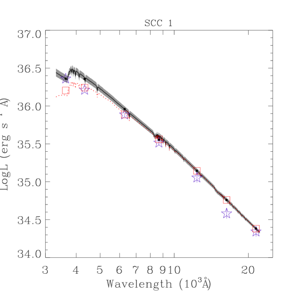
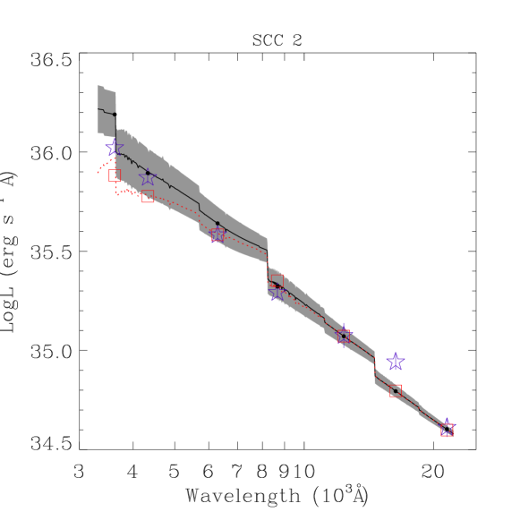
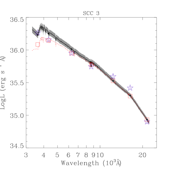
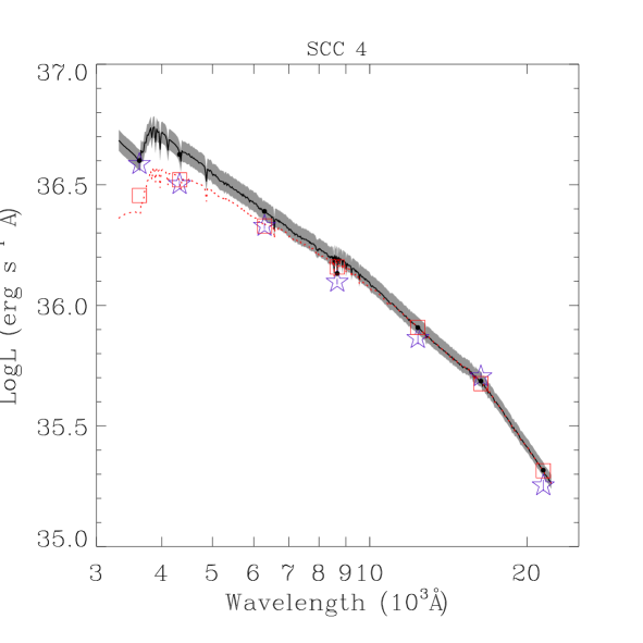
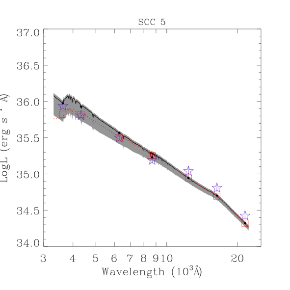
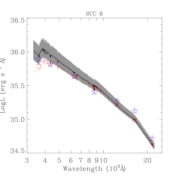

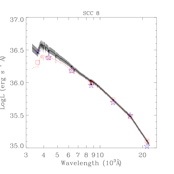
SCC #1 is associated with an age of 6 Myr, extinction and a mass of . SCC #2 is older (10 Myr) but with similar extinction and mass ( and ). These two SCCs coincide with the brightest H II region in the emission line maps H II #5 (Section 4.2.2). Next to these complexes and towards the west is SCC #3. This is the youngest (3 Myr old) and most extinguished ( mag) of them all, and lies in between two H II regions (#5 and #4). The remaining five SCCs are 10 Myr old with masses . Three of them (SCC #5, SCC #6 and SCC #8) are related to a slightly displaced H II region. SCC #8 is the second most massive cluster complex ( ) and its companion H II region is the second brightest in the emission line maps.
For six of the eight SCCs the average change on the adopted age and extinction due to the model uncertainty is lower than 5% and 14% respectively. The adopted age variation was the same independently of the uncertainty definition used. The 5% uncertainty in the models on the other hand, causes a 0.11 mag decrease in the adopted extinction, which is twice the change induced by the uncertainty due to the time variation of the luminosity. For the other two SCCs the uncertainty of the model lead to a 5 Myr increment in both SCCs adopted ages and a 40% and 20% change in the extinction value respectively.
5.2.4 H II regions
The H II regions in this galaxy are being photoionised by star clusters that are 10 Myr old or younger, as shown in Section 3.2 (Figure 6) through the analysis of the cell’s value. All of them present that would be expected if ionisation of the gas was performed by photons, rather than shocks. The and U-B colour of a modelled SSP are used as tools to date the stellar populations that ionise H II regions (Dottori, 1981; Chiosi et al., 1986; Stasińska & Leitherer, 1996; Cid Fernandes et al., 2003; Martín-Manjón et al., 2008; Hancock et al., 2008; Martín-Manjón et al., 2012). This procedure relies on:
-
1.
The stellar extinction is either negligible or fixed and known.
-
2.
The observed H II region encloses its ionising SCC.
-
3.
The colours of the H II region are representative of the stellar ionising source.
-
4.
And the effect of an underlying stellar population is not included in the equivalent width of .
In Section 3.2 we showed that extinction in the star-forming region of this galaxy is nearly uniform and can be considered negligible, therefore the first premise is fulfilled. In order to estimate the ages of the star clusters responsible for the ionisation of the H II regions we followed the commonly used hypothesis that the other two premises are verified as well (Álvarez-Álvarez et al., 2015, ME00). This idea has been previously adopted by ME00, who dated the H II regions by comparing their U-B colour and with those predicted by SSP models from Starburst99 (Leitherer et al., 1999).
The vs U-B diagram is shown in Figure 9. The 6 HII regions with measured U-B colour are shown as blue stars. We can compare their position in the diagram with the trace of the evolution of a PopStar SSP model from 0.1 Myr to 9 Myr old. We can see that the contribution of an older stellar population in both the measured U-B colour and the seems to be negligible. The and the U-B colours of the six H II regions are compatible with a and a old SSP model respectively.
We have compared our results with those obtained by ME00 who also find a 5 Myr old age for the ionising clusters from the . But when the U-B colour of the H II regions is used, then the ionising cluster is matched with a Myr old model SSP, twice the age given by ME00 (). This difference (which can be as high as 0.25 mag) might be explained by the fact that PopStar models predict a slightly redder () U-B colour than Starburst99.
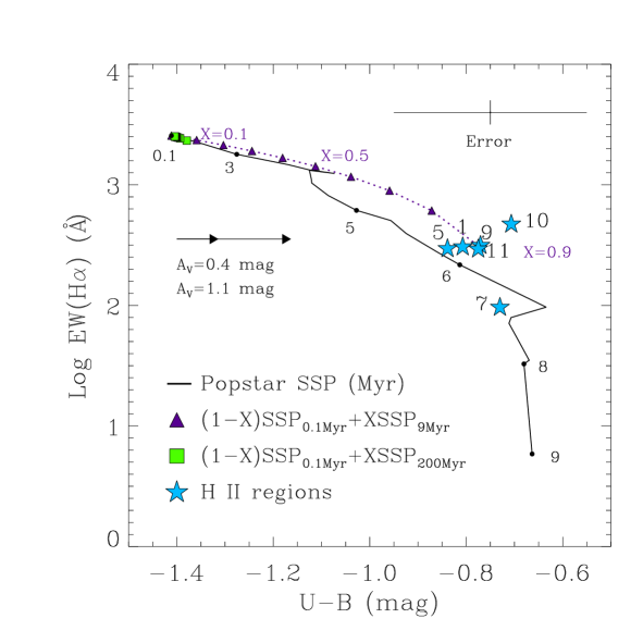
PopStar models consider that for a SSP with Z=0.004 the Wolf-Rayet phase starts at 3 Myr and ends at 5 Myr. If the star clusters that ionise the H II regions are 5 Myr old - as estimated from the - then the presence of Wolf-Rayet stars cannot be ruled out. This idea is supported by the U-B colour of the H II regions (), since the characteristic U-B colour of Wolf-Rayet stars is 0.7 mag according to the sample of Wolf-Rayet stars collected by Paul Crowhter999http://pacrowther.staff.shef.ac.uk/WRcat/. The intense emission from H II regions #5, #8, #10 and #11 (Table 10) implies that they are being photoionised by more than ten massive O7 V stars (Table 12) and therefore, these regions are candidates to host Wolf-Rayet stars. Another clue pointing to these H II regions as probably photoionised by Wolf-Rayet stars is their high excitation, deduced from their values. In Section 3.2, we showed that the ratio is a good excitation indicator in the star-forming activity of this galaxy, and the appearance of Wolf-Rayet stars in star clusters is likely to increase the nebular excitation of the surrounding H II region (Buckalew et al., 2005). This is in agreement with the results obtained by Méndez & Esteban (2000), and consistent with the identification of in the spectrum of the galaxy by Kunth & Joubert (1985); Vacca & Conti (1992) and Schaerer et al. (1999).
6 DISCUSSION AND CONCLUSIONS
6.1 Stellar populations across the galaxy
As shown in Sections 4.1 and 5.1, the galaxy is formed by a disk dominated by the light of a 1.5 Gyr old stellar population, which has a photometric mass of , and is directly observed in the East and West zones of the galaxy. A Myr old star-forming event is located at its centre, formed by eight massive SCCs (, see Table 13) and twelve H II regions (Figures 2 and 7). Since all the objects are younger than 10 Myr old, we can consider the idea of an instantaneous star-formation episode. This result supports the assumption that the star-formation triggering mechanism of isolated H II galaxies is stochastic, as proposed by Telles (2010). So despite the fact that the star clusters appear to be aligned, it seems that the star formation has not propagated along this apparent alignment.
The mass of the SCCs is and their total mass is , which represents only 8% of the estimated mass in the Centre zone (Table 13). SCCs are concentrated at the Centre zone of the galaxy, while the emission and H II regions are distributed in the Centre, North and South zones (Figure 2). H II regions -with the exception of #1- are displaced from the positions of the SCCs, so determining their ionising source is very difficult. H II region #1 is the brightest of them all and encloses two star cluster complexes, SCC #1 and SCC #2. Since SCC #1 is younger and more massive than its companion, it emits more ionising photons, which leads us to believe that SCC #1 dominates the evolution of the H II region. Still, further spectroscopic information is required to accurately determine the age and kinematics of the H II region.
6.2 SCCs red colours
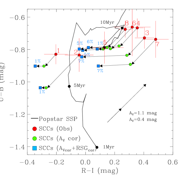
Figure 10 shows the position of the SCCs before (red circles) and after (green circles) correction by its associated SSP fit extinction value in the optical-NIR U-B vs R-I and NIR I-J vs J-H diagrams. The evolutionary track of an extinction-free PopStar SSP model is also overplotted. The SCCs U-B colour corresponds to a SSP younger than 10 Myr even before being corrected by extinction being the bluest SCCs (#1 and #2) the ones coinciding with the brightest H II region (H II #5). On the other hand, the SCCs R-I colour is redder than what the models predict, even after having been corrected by extinction. A similar excess in the R-I colour was observed previously by Díaz et al. (2000) in a sample of nuclear star clusters. They suggested that this red excess could be attributed to Red Supergiant Stars not being properly taken into consideraton in SSP models. This issue will be addressed further in Section (6.2.1).
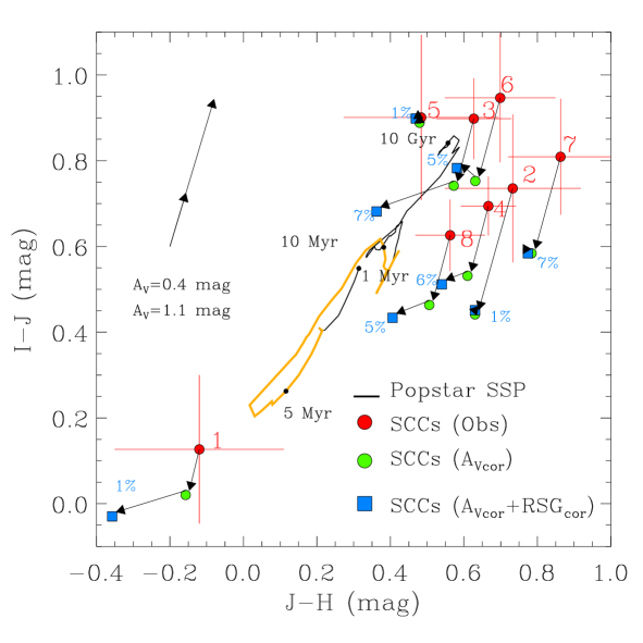
H is the band most affected by the emission lines; J-H turns bluer, thus moving the evolutionary track towards the left. The emission lines contribution decreases with time, becoming negligible for a 10 Myr old SSP. SCC #1 is an outlier at the bottom-left corner of the I-J vs J-H diagram. Its position suggests that its flux is affected by nebular emission lines, which is to be expected for the estimated age of 6 Myr. The rest of the SCCs are found grouped at the top-right red area of the diagram ( mag and mag), closer to the evolutionary track at ages older than 10 Myr. Even after being corrected by extinction, four of the SCCs (#2, #4, #7 and #8) are still apart from the evolutionary track, and the rest (with the exception of SCC #1) are consistent with ages greater than 10 Myr, which contradicts the optical-NIR diagram.
Reddening of SCCs NIR (I, J, H and K) bands has been observed previously in the literature (Origlia et al., 1999; Vázquez & Leitherer, 2005; Reines et al., 2008; Reines et al., 2010; Adamo et al., 2010; Gazak et al., 2013). The mismatch between young stellar populations observed NIR colours and the models was first noticed by Origlia et al. (1999) when studying the integrated colours of BCD galaxies. Subsequent studies on resolved stellar clusters in a variety of star-forming galaxies have come across this problem. Ad hoc mechanisms have been proposed to explain it, such as extended red emission (ERE, Reines et al., 2008; Adamo et al., 2010), nebular continuum and emission lines (Reines et al., 2010), the use of large apertures to compute the photometry (Bastian et al., 2014), and that the number of RSG stars predicted by the models might be underestimated (Origlia et al., 1999; Vázquez & Leitherer, 2005; Gazak et al., 2013), being this last one the most popular explanation.
The 10 Myr estimated age for the SCCs (epoch at which the RSG population has already begun its maximum contribution to the SCC light) supports the idea that the mismatch between the colour of the SCCs and the models is related to the number of RSG predicted by the models. Therefore, motivated by Gazak et al. (2013), who found that the J-H colour of a sample of stellar clusters was better reproduced by SSP models after increasing the number of RSG stars in them, we decided to analyse whether a dearth of RSG stars in PopStar models could be the cause of the mismatch between the models and the photometry of our SCCs.
6.2.1 Dearth of RSG stars in the models?
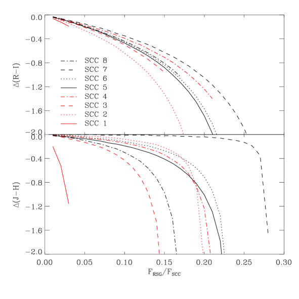
We can test whether the models underestimate the number of RSG stars by removing the contribution of a number of RSG from the luminosity of the SCCs and estimating the resulting NIR colours. Considering that the metallicity of the galaxy might determine the spectral type of its RSGs (Massey & Olsen, 2003), we chose a K5-7 RSG star of the low metallicity Small Magellanic Cloud (Massey & Olsen, 2003) as prototype for the RSG stars in Tol 02 and its characteristics are shown in Table 14. We subtracted up to 20 times the luminosity of the prototype RSG star from the observed luminosity of each SCC. The subtracted R band luminosity contribution represents a fraction of the SCC total luminosity and is used as a measure to compare the colour changes suffered by different SCCs, independently of their masses. These colour changes are described below.
| Star ID (Massey & Olsen, 2003): 059426 | |||
| Star ID (Prevot et al., 1983) : PMMR 158 | |||
| Coords: R.A. 010430.28Dec. -72°04′36.1″ | |||
| Radial velocity: | |||
| Spectral Type and Luminosity class: K5-7 I | |||
| U | B | R | I |
| J | H | K | |
The subtraction of RSG stars turns out to be irrelevant for U-B. The change it produces in the colour is , which is negligible compared to the increase of 0.7 magnitudes in U-B when the SSP ages from 2 to 6 Myr. On the contrary, when the subtracted R luminosity represents 20% of the observed luminosity (), that turns R-I bluer by , larger than the change of the R-I colour of an extinction free SCC during its lifetime (-0.1 mag < R-I < 0.7 mag). This rapid change to the blue by artificially discounting RSG stars is shown in the top panel of Figure 11. The J-H colour is also sensitive to the presence of RSG stars, as shown in the bottom panel of Figure 11. This figure shows that when the RSG stars R luminosity represents of the SCCs R band luminosity, the change suffered by the J and H luminosities moves 0.1 mag to the blue the J-H colours of six clusters.
The change in I-J colour due to the subtraction of the RSG stars is more complex. Only four SCCs become bluer when the RSG stars are subtracted from them, while the remaining three (#1, #2 and #6) become redder. SCCs #1 and #2 are located inside the brightest H II region, and the SCC #6 aperture overlaps with the aperture of H II region #7 in of area. These three complexes can be considered to be affected by the emission lines. Therefore the subtraction of the RSG stellar light enhances the effect of the contamination by the nebular emission lines and produces the curious effect of a redder colour of the SCC.
The significance of the RSG stars to the SCC colours is shown in Figure 10. Each SCC is tagged with its ID number next to the original colour (red circle) and the fraction of the cluster subtracted R band light (as a percent) next to the SCC colour after a number of RSG stars has been subtracted (blue squares). The pointing of the arrows in the figure shows that the subtraction of the light from the RSG stars moves the SCCs away from the models, with the exception of SCC #4 and #8. When the flux of these two SCCs is subtracted from the light of RSG stars their resultant colours are in better agreement with the prediction of the models.
It is clear from the figure that the mismatch between the SSP models and the photometry of the SCCs can be caused by an underestimate of the number of RSG stars in the evolutionary tracks only for SCCs #4 and #8.
In summary:
-
1.
The RSG stars do not contribute to the U-B colour.
-
2.
The increase in the number of RSG stars in a SCC reddens both J-H and R-I, being the latter colour the most affected one.
Therefore, at least for six of the eight SCCs a “simple” change in the number of RSG stars of the models is not capable of reproducing the observations. The problem seems to be more likely the modelling of the SED slope in the NIR range m to 2.5 m, where the luminosity of a SSP model decreases steadily as the wavelength increases. But if the SSP modelled luminosity increased at H, the J-H colour would redden, thus better reproducing the observation.
A NIR continuum spectrum with a luminosity increase that peaks towards the H band and then decreases towards the K band is observed in some metal rich star-forming spiral galaxies (Martins et al., 2013). To assess whether this behaviour could be expected also in low metallicity smaller systems like H II galaxies (in particular Tol 02) high spatial and spectral resolution NIR data on each of the SCCs would be required in order to confirm this hypothesis.
6.3 CONCLUSIONS
A detailed study of the star-forming regions and star cluster complexes in the H II galaxy Tol 02 was performed using a broad (U, B, R, I, J, H, K, and deep ) set of images of the galaxy. The map is presented for the first time for this galaxy. These images, combined with SSP PopStar models, have allowed us to conclude that:
-
•
The galaxy can be represented by a disk whose light is dominated by an extinction-free 1.5 Gyr old stellar population with a total mass of , and a Myr old central starburst whose light spreads towards the North and South of the galaxy, dominating over the red light of the disk component.
-
•
The star-forming region of this galaxy is formed by twelve bright () H II regions, the most luminous of which is a giant H II region (). The U-B colour, and values of the four brightest H II regions suggest that these H II regions might be photoionised by clusters containing Wolf-Rayet stars. This is in agreement with the results obtained by Méndez & Esteban (2000), and consistent with the identification of in the spectrum of the galaxy by Kunth & Joubert (1985); Vacca & Conti (1992) and Schaerer et al. (1999).
-
•
Eight massive () SCC located in the brightest H II regions were identified, however the physical connection between each H II region and the SCCs is not clear. The crowding of the H II regions and SCCs makes it impossible to determine to which H II region a given SCC relates. Fitting SEDs of model SSP using PopStar is consistent with six of the SCC being 10 Myr old, so expected to contain RSG stars, while the other two are 3 and 5 Myr old and therefore are Wolf-Rayet cluster candidates.
-
•
The young ages ascribed to the SCCs and H II regions ( Myr) suggest an instantaneous and stochastic star formation mode that depends on short scale inhomogeneities of the interstellar medium.
An ad-hoc experiment subtracting a combination of typical RSG stars indicates that the R-I excess observed in the SCCs is well explained if the models predict an incorrect number of RSG stars, as previously suggested by Díaz et al. (2000).
-
•
The I-J and J-H colours of SCCs #4 and #8 (most massive clusters identified) can be explained if the models are underestimating the number of RSG stars. However, the NIR colours of the remaining SCCs can not be explained in the same way.
This article presents the first results of a project aimed at characterising the spatially resolved dominant stellar populations in six low metallicity H II galaxies, which helps to understand whether these galaxies with intensive star-formation are prone to form massive star clusters and if their star formation process is stochastic or sequentially induced, therefore providing a better understanding of the star-formation process undergone in low metallicity systems.
Acknowledgements
The authors wish to thank an anonymous referee whose recommendations greatly improved the clarity of the paper. AT-C is thankful to Patricio Lagos, Erique Pérez, Lino Rodríguez-Merino, Abraham Luna, Mercedes Mollá, Polychronis Papaderos, Nate Bastian and Divakara Mayya for fruitful discussions, and to her sister Nora for a careful reading of the manuscript. We also would like to thank the Time Allocation Committee and the very helpful supporting staff at SOAR.
This research has made use of the NASA/IPAC Extragalactic Database (NED) which is operated by the Jet Propulsion Laboratory, California Institute of Technology, under contract with the National Aeronautics and Space Administration.
This work was supported by CONACyT (México) student fellowship grant 46360 and research project numbers CB-2011/167281. Partial financial support from projects: AYA2013-47742-C4-3-P from the Ministerio de Economía y Competitividad (MINECO, Spain) and SELGIFS: FP7-PEOPLE-2013-IRSES-612701 the Research Executive Agency (REA, EU) is acknowledged. Ana Torres-Campos is grateful to the hospitality of the Departamento de Física Teórica in Madrid and the Observatorio Nacional in Rio, during work visits when part of this work was completed.
References
- Adamo et al. (2010) Adamo A., Östlin G., Zackrisson E., Hayes M., Cumming R. J., Micheva G., 2010, MNRAS, 407, 870
- Adamo et al. (2011) Adamo A., Östlin G., Zackrisson E., Papaderos P., Bergvall N., Rich R. M., Micheva G., 2011, MNRAS, 415, 2388
- Álvarez-Álvarez et al. (2015) Álvarez-Álvarez M., Díaz A. I., Terlevich E., Terlevich R., 2015, MNRAS, 451, 3173
- Anders & Fritze-v. Alvensleben (2003) Anders P., Fritze-v. Alvensleben U., 2003, A&A, 401, 1063
- Ashley et al. (2017) Ashley T., Simpson C. E., Elmegreen B. G., Johnson M., Pokhrel N. R., 2017, AJ, 153, 132
- Baldwin & Stone (1984) Baldwin J. A., Stone R. P. S., 1984, MNRAS, 206, 241
- Bastian et al. (2014) Bastian N., et al., 2014, MNRAS, 444, 3829
- Bergvall et al. (1999) Bergvall N., Rönnback J., Masegosa J., Östlin G., 1999, A&A, 341, 697
- Bertin & Arnouts (1996) Bertin E., Arnouts S., 1996, A&AS, 117, 393
- Bessell et al. (1998) Bessell M. S., Castelli F., Plez B., 1998, A&A, 333, 231
- Brennan et al. (2016) Brennan R., et al., 2016, preprint, (arXiv:1607.06075)
- Buckalew et al. (2005) Buckalew B. A., Kobulnicky H. A., Dufour R. J., 2005, ApJS, 157, 30
- Cairós et al. (2001) Cairós L. M., Vílchez J. M., González Pérez J. N., Iglesias-Páramo J., Caon N., 2001, ApJS, 133, 321
- Cairós et al. (2003) Cairós L. M., Caon N., Papaderos P., Noeske K., Vílchez J. M., García Lorenzo B., Muñoz-Tuñón C., 2003, ApJ, 593, 312
- Calzetti et al. (2010) Calzetti D., et al., 2010, ApJ, 714, 1256
- Cardelli et al. (1989) Cardelli J. A., Clayton G. C., Mathis J. S., 1989, ApJ, 345, 245
- Chiosi et al. (1986) Chiosi C., Bertelli G., Bressan A., 1986, Mem. Soc. Astron. Italiana, 57, 507
- Cid Fernandes et al. (2003) Cid Fernandes R., Leão J. R. S., Lacerda R. R., 2003, MNRAS, 340, 29
- Díaz et al. (2000) Díaz A. I., Álvarez M. Á., Terlevich E., Terlevich R., Sánchez Portal M., Aretxaga I., 2000, MNRAS, 311, 120
- Dottori (1981) Dottori H. A., 1981, Ap&SS, 80, 267
- Doublier et al. (1999) Doublier V., Caulet A., Comte G., 1999, A&AS, 138, 213
- Engelbracht et al. (2008) Engelbracht C. W., Rieke G. H., Gordon K. D., Smith J.-D. T., Werner M. W., Moustakas J., Willmer C. N. A., Vanzi L., 2008, ApJ, 678, 804
- Gazak et al. (2013) Gazak J. Z., Bastian N., Kudritzki R.-P., Adamo A., Davies B., Plez B., Urbaneja M. A., 2013, MNRAS, 430, L35
- Gil de Paz et al. (2003) Gil de Paz A., Madore B. F., Pevunova O., 2003, ApJS, 147, 29
- Greis et al. (2016) Greis S. M. L., Stanway E. R., Davies L. J. M., Levan A. J., 2016, MNRAS, 459, 2591
- Hamuy et al. (1992) Hamuy M., Walker A. R., Suntzeff N. B., Gigoux P., Heathcote S. R., Phillips M. M., 1992, PASP, 104, 533
- Hancock et al. (2008) Hancock M., Smith B. J., Giroux M. L., Struck C., 2008, MNRAS, 389, 1470
- Jacoby et al. (1987) Jacoby G. H., Africano J. L., Quigley R. J., 1987, PASP, 99, 672
- Kehrig et al. (2004) Kehrig C., Telles E., Cuisinier F., 2004, AJ, 128, 1141
- Kewley et al. (2001) Kewley L. J., Dopita M. A., Sutherland R. S., Heisler C. A., Trevena J., 2001, ApJ, 556, 121
- Kunth & Joubert (1985) Kunth D., Joubert M., 1985, A&A, 142, 411
- Kunth & Östlin (2000) Kunth D., Östlin G., 2000, A&ARv, 10, 1
- Kunth et al. (1988) Kunth D., Maurogordato S., Vigroux L., 1988, A&A, 204, 10
- Lagos et al. (2007) Lagos P., Telles E., Melnick J., 2007, A&A, 476, 89
- Lagos et al. (2011) Lagos P., Telles E., Nigoche-Netro A., Carrasco E. R., 2011, AJ, 142, 162
- Leitherer et al. (1999) Leitherer C., et al., 1999, ApJS, 123, 3
- Lelli et al. (2014) Lelli F., Verheijen M., Fraternali F., 2014, MNRAS, 445, 1694
- Loh et al. (2011) Loh E. D., Baldwin J. A., Curtis Z. K., Ferland G. J., O’Dell C. R., Fabian A. C., Salomé P., 2011, ApJS, 194, 30
- Martín-Manjón et al. (2008) Martín-Manjón M. L., Mollá M., Díaz A. I., Terlevich R., 2008, MNRAS, 385, 854
- Martín-Manjón et al. (2012) Martín-Manjón M. L., Mollá M., Díaz A. I., Terlevich R., 2012, MNRAS, 420, 1294
- Martins et al. (2013) Martins L. P., Rodríguez-Ardila A., Diniz S., Riffel R., de Souza R., 2013, MNRAS, 435, 2861
- Massey & Olsen (2003) Massey P., Olsen K. A. G., 2003, AJ, 126, 2867
- Mayya (1994) Mayya Y. D., 1994, AJ, 108, 1276
- Mayya et al. (2005) Mayya Y. D., Carrasco L., Luna A., 2005, ApJ, 628, L33
- Melo et al. (2005) Melo V. P., Muñoz-Tuñón C., Maíz-Apellániz J., Tenorio-Tagle G., 2005, ApJ, 619, 270
- Méndez & Esteban (2000) Méndez D. I., Esteban C., 2000, A&A, 359, 493
- Micheva et al. (2013) Micheva G., Östlin G., Bergvall N., Zackrisson E., Masegosa J., Marquez I., Marquart T., Durret F., 2013, MNRAS, 431, 102
- Mollá et al. (2009) Mollá M., García-Vargas M. L., Bressan A., 2009, MNRAS, 398, 451
- Mould et al. (2000) Mould J. R., et al., 2000, ApJ, 529, 786
- Muñoz-Mateos et al. (2009) Muñoz-Mateos J. C., et al., 2009, ApJ, 703, 1569
- Origlia et al. (1999) Origlia L., Goldader J. D., Leitherer C., Schaerer D., Oliva E., 1999, ApJ, 514, 96
- Osterbrock & Ferland (2006) Osterbrock D. E., Ferland G. J., 2006, Astrophysics of gaseous nebulae and active galactic nuclei
- Papaderos et al. (1996) Papaderos P., Loose H.-H., Thuan T. X., Fricke K. J., 1996, A&AS, 120, 207
- Persson et al. (1998) Persson S. E., Murphy D. C., Krzeminski W., Roth M., Rieke M. J., 1998, AJ, 116, 2475
- Pickles (1998) Pickles A. J., 1998, PASP, 110, 863
- Prevot et al. (1983) Prevot L., Martin N., Rebeirot E., Maurice E., Rousseau J., 1983, A&AS, 53, 255
- Raimann et al. (2000) Raimann D., Bica E., Storchi-Bergmann T., Melnick J., Schmitt H., 2000, MNRAS, 314, 295
- Reines et al. (2008) Reines A. E., Johnson K. E., Hunt L. K., 2008, AJ, 136, 1415
- Reines et al. (2010) Reines A. E., Nidever D. L., Whelan D. G., Johnson K. E., 2010, ApJ, 708, 26
- Rich et al. (2012) Rich R. M., Collins M. L. M., Black C. M., Longstaff F. A., Koch A., Benson A., Reitzel D. B., 2012, Nature, 482, 192
- Rodríguez-Merino et al. (2011) Rodríguez-Merino L. H., Rosa-González D., Mayya Y. D., 2011, ApJ, 726, 51
- Sargent & Searle (1970) Sargent W. L. W., Searle L., 1970, ApJ, 162, L155
- Schaerer et al. (1999) Schaerer D., Contini T., Pindao M., 1999, A&AS, 136, 35
- Skrutskie et al. (2006) Skrutskie M. F., et al., 2006, AJ, 131, 1163
- Smith et al. (1976) Smith M. G., Aguirre C., Zemelman M., 1976, ApJS, 32, 217
- Stasińska & Leitherer (1996) Stasińska G., Leitherer C., 1996, ApJS, 107, 661
- Stone & Baldwin (1983) Stone R. P. S., Baldwin J. A., 1983, MNRAS, 204, 347
- Telles (2010) Telles E., 2010, in B. Smith, J. Higdon, S. Higdon, & N. Bastian ed., Astronomical Society of the Pacific Conference Series Vol. 423, Galaxy Wars: Stellar Populations and Star Formation in Interacting Galaxies. p. 65 (arXiv:0908.2966)
- Telles & Terlevich (1995) Telles E., Terlevich R., 1995, MNRAS, 275, 1
- Telles & Terlevich (1997) Telles E., Terlevich R., 1997, MNRAS, 286, 183
- Terlevich et al. (1991) Terlevich R., Melnick J., Masegosa J., Moles M., Copetti M. V. F., 1991, A&AS, 91, 285
- Terlevich et al. (2004) Terlevich R., Silich S., Rosa-González D., Terlevich E., 2004, MNRAS, 348, 1191
- Thuan (1983) Thuan T. X., 1983, ApJ, 268, 667
- Vacca & Conti (1992) Vacca W. D., Conti P. S., 1992, ApJ, 401, 543
- Valdes (1982) Valdes F., 1982, National Optical Astronomy Observatories
- Vázquez & Leitherer (2005) Vázquez G. A., Leitherer C., 2005, ApJ, 621, 695
- Westera et al. (2004) Westera P., Cuisinier F., Telles E., Kehrig C., 2004, A&A, 423, 133
- Whitford (1958) Whitford A. E., 1958, AJ, 63, 201
Appendix A APENDIX A. FLUX CALIBRATION
A.1 Broad band flux calibration
The magnitude of the standard star is related to the star image counts rate:
| (4) |
where is the standard star magnitude, is the number of counts per second received by the detector from the standard star, is the extinction coefficient at wavelength , is the airmass at which the standard star was observed and is the zeropoint, a constant that relates the standard star image counts per second to the published magnitude value. Equation 4 is solved for the standard stars observed and a median value for is obtained as:
| (5) |
The observed magnitude of an object with total counts per second inside an aperture with N pixels is:
| (6) |
where is the sky counts per second, and the object magnitude uncertainty is given by:
| (7) |
where is the counts per second of the object and its uncertainty is given by:
| (8) |
The magnitude to flux conversion is computed using the relation:
| (9) |
where is the flux of Vega (Bessell et al., 1998).
A.2 Narrow band flux calibration
For the narrow band flux calibration we followed Jacoby et al. (1987), where the standard star flux is given by equation (Jacoby et al., 1987):
| (10) |
in units of []. Where is the monochromatic flux above the atmosphere for the standard star in units of [] and is the narrow band filter transmission curve.
The CCD system sensitivity (in units of [erg cm-2 s-1 counts-1]) was computed using the standard stars images:
| (11) | |||
| (12) |
is the count (photon) rate101010The number of counts of the standard stars is determined using the daophot and phot tasks from the noao.digiphot.daophot package., is the airmass and is the extinction coefficient111111The extinction coefficient curve is the Cerro Tololo International Observatory (CTIO) one used in IRAF’s task extinction (Stone & Baldwin, 1983; Baldwin & Stone, 1984). for the narrow band filter image of the standard star, is the standard star counts rate uncertainty () and is the uncertainty of the sky counts per second.
The targe flux is related to the sensitivity of the system by:
| (13) |
where is the target flux observed in the narrow band, is the count rate from the target at any pixel of interest, is the airmass at which the target was observed and is the extinction coefficient for the narrow band filter. The emission line flux emitted by the target (in this case a galaxy) is essentially a delta function over the filter bandpass centre at the wavelength of the emission line, L. Then,
| (14) |
where denotes the filter transmission at the emission line wavelength. So, if we substitute equation 13 in equation 14 we obtain the observed flux of the galaxy:
| (15) |
where is the flux per count in the galaxy image, in units of []. As this equation states, to flux calibrate the flat corrected galaxy image we just have to multiply it by the flux per count coefficient (). The counts to flux transformation equations are:
| (16) |
The counts per second inside an object aperture with N pixels is given by:
| (17) | |||
| (18) |
where is the counts per second in pixel i, sky is the mean sky value, is the standard deviation of the sky measurement and the number of median combined galaxy images. Finally flux of the object () and its uncertainty () in units of erg is calculated as:
| (19) | |||
| (20) |
If you want to present additional material which would interrupt the flow of the main paper, it can be placed in an Appendix which appears after the list of references.