MBL-mobile: Quantum engine based on many-body localization

Abstract

Many-body-localized (MBL) systems do not thermalize under their intrinsic dynamics. The athermality of MBL, we propose, can be harnessed for thermodynamic tasks. We illustrate this ability by formulating an Otto engine cycle for a quantum many-body system. The system is ramped between a strongly localized MBL regime and a thermal (or weakly localized) regime. The difference between the energy-level correlations of MBL systems and of thermal systems enables mesoscale engines to run in parallel in the thermodynamic limit, enhances the engine’s reliability, and suppresses worst-case trials. We estimate analytically and calculate numerically the engine’s efficiency and per-cycle power. The efficiency mirrors the efficiency of the conventional thermodynamic Otto engine. The per-cycle power scales linearly with the system size and inverse-exponentially with a localization length. This work introduces a thermodynamic lens onto MBL, which, having been studied much recently, can now be considered for use in thermodynamic tasks.

Many-body localization (MBL) has emerged as a unique phase in which an isolated interacting quantum system resists internal thermalization for long times. MBL systems are integrable and have local integrals of motion Huse_14_phenomenology , which retain information about initial conditions for long times or even indefinitely KjallIsing . This and other aspects of MBL were recently observed experimentally Schreiber_15_Observation ; Kondov_15_Disorder ; Ovadia_15_Evidence ; Choi_16_Exploring ; Luschen_17_Signatures ; Kucsko_16_Critical ; Smith_16_Many ; Bordia_17_Probing . In contrast, in thermalizing isolated quantum systems, information and energy can diffuse easily. Such systems obey the eigenstate thermalization hypothesis (ETH) Deutsch_91_Quantum ; Srednicki_94_Chaos ; Rigol_07_Relaxation ; rigol-dunjko-olshanii .

A tantalizing question is whether the unique properties of MBL could be utilized. So far, MBL has been proposed to be used as robust quantum memories Nandkishore_15_MBL . We believe, however, that the potential of MBL is much greater. MBL systems behave athermally, and athermality (lack of thermal equilibrium) facilitates thermodynamic tasks Janzing_00_Thermodynamic ; Dahlsten_11_Inadequacy ; Aberg_13_Truly ; Brandao_13_Resource ; Horodecki_13_Fundamental ; Egloff_15_Measure ; Goold_15_review ; Gour_15_Resource ; YungerHalpern_16_Beyond ; Deffner_16_Quantum ; Wilming_17_Third . When a cold bath is put in contact with a hot environment, for instance, work can be extracted from the heat flow. Could MBL’s athermality have thermodynamic applications?

We present one by formulating, analyzing, and numerically simulating an Otto engine cycle for a quantum many-body system that has an MBL phase. The engine contacts a hot bath and a narrow-bandwidth cold bath, as sketched in Fig. 1. This application unites the growing fields of quantum thermal machines Geusic_maser_67 ; del_Campo_14_Super ; Brunner_15_Ent_fridge ; Binder_15_Quantacell ; Woods_15_Maximum ; Gelbwaser_15_Strongly ; Song_16_polariton_engine ; Tercas_16_Casimir ; PerarnauLlobet_16_Work ; Kosloff_17_QHO ; Lekscha_16_Quantum ; Jaramillo_16_Quantum ; Gelbwaser_18_Single and MBL BAA ; Oganesyan_07_Level_stats ; Pal_Huse_10_MBL ; Huse_14_phenomenology ; Nandkishore_15_MBL ; serbynmoore . Our proposal could conceivably be explored in ultracold-atom Schreiber_15_Observation ; Kondov_15_Disorder ; Choi_16_Exploring ; Luschen_17_Signatures ; Bordia_17_Probing , nitrogen-vacancy-center Kucsko_16_Critical , trapped-ion Smith_16_Many , and possibly doped-semiconductor Kramer_93_Localization experiments.

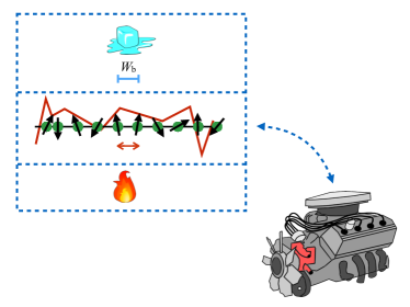
Figure 1: Schematic of MBL engine: We formulate an Otto engine cycle for a many-body quantum system that exhibits an MBL phase. We illustrate the engine with a spin chain (green dots and black arrows). A random disorder potential (jagged red line) localizes the particles. Particles interact and hop between sites (horizontal red arrows). Consider strengthening the interactions and the hopping frequency. The system transitions from strong localization to a thermal phase or to weak localization. The engine thermalizes with a hot bath (flames) and with a cold bath (ice cube). The cold bath has a small bandwidth, $W_{\rm b}$, to take advantage of small energy gaps’ greater prevalence in the highly localized regime.

Our engine relies on two properties that distinguish MBL from thermal systems: its spectral correlations Sivan_87_Energy ; serbynmoore and its localization. The spectral-correlation properties enable us to build a mesoscale level-statistics engine. The localization enables us to link mesoscale engines together, creating a large engine with an extensive work output.

Take an interacting finite spin chain as an example. Consider the statistics of the gaps between consecutive energy eigenvalues far from the energy band’s edges. A gap distribution $P(\delta)$ encodes the probability that any given gap has size $\delta$. The MBL gap distribution enables small (and large) gaps to appear much more often than in ETH spectra D'Alessio_16_From . This difference enables MBL to enhance our quantum many-body Otto cycle.

Let us introduce the MBL and ETH distributions in greater detail. Let $\left\langle\delta\right\rangle_{E}$ denote the average gap at the energy $E$. MBL gaps approximately obey Poisson statistics Oganesyan_07_Level_stats ; D'Alessio_16_From :

$$P_{\rm MBL}^{(E)}(\delta)\approx\frac{1}{\left\langle\delta\right\rangle_{E}}e^{-\delta/\left\langle\delta\right\rangle_{E}}\,.$$ (1)

Any given gap has a decent chance of being small: As $\delta\to 0$, $P_{\rm MBL}^{(E)}(\delta)\to\frac{1}{\left\langle\delta\right\rangle_{E}}>0$. Neighboring energies have finite probabilities of lying close together: MBL systems’ energies do not repel each other, unlike thermal systems’ energies. Thermalizing systems governed by real Hamiltonians obey the level statistics of random matrices drawn from the Gaussian orthogonal ensemble (GOE) Oganesyan_07_Level_stats :

$$P_{\rm GOE}^{(E)}(\delta)\approx\frac{\pi}{2}\frac{\delta}{\left\langle\delta\right\rangle_{E}^{2}}\>e^{-\frac{\pi}{4}\delta^{2}/\left\langle\delta\right\rangle_{E}^{2}}\,.$$ (2)

Unlike in MBL spectra, small gaps rarely appear: As $\delta\to 0$, $P_{\rm GOE}^{(E)}(\delta)\to 0$.

MBL’s athermal gap statistics should be construed as a thermodynamic resource, we find, as athermal quantum states have been Janzing_00_Thermodynamic ; Dahlsten_11_Inadequacy ; Aberg_13_Truly ; Brandao_13_Resource ; Horodecki_13_Fundamental ; Egloff_15_Measure ; Goold_15_review ; Gour_15_Resource ; YungerHalpern_16_Beyond ; Deffner_16_Quantum ; Wilming_17_Third . In particular, MBL’s athermal gap statistics improve our engine’s reliability: The amount $W_{\rm tot}$ of work extracted by our engine fluctuates relatively little from successful trial to successful trial. Athermal statistics also lower the probability of worst-case trials, in which the engine outputs net negative work, $W_{\rm tot}<0$. Furthermore, MBL’s localization enables the engine to scale robustly: Mesoscale “subengines” can run in parallel without disturbing each other much, due to the localization inherent in MBL. Even in the thermodynamic limit, an MBL system behaves like an ensemble of finite, mesoscale quantum systems, due to its local level correlations Sivan_87_Energy ; imryma ; Syzranov_17_OTOCs . Any local operator can probe only a discrete set of sharp energy levels, which emerge from its direct environment.

This paper is organized as follows. Section I contains background about the Otto cycle and about quantum work and heat. In Sec. II, we introduce the mesoscopic MBL engine. In Sec. IIA, we introduce the basic idea with a qubit (two-level quantum system). In Sec. IIB, we scale the engine up to a mesoscopic chain tuned between MBL and ETH regimes. In Sec. IIC, we calculate the engine’s work output and efficiency. In Sec. III, we argue that the mesoscopic segments can be combined into a macroscopic MBL system while operating in parallel. In Sec. IV, we discuss limitations on the speed at which the engine can be run and, consequently, the engine’s power. This leads us to a more careful consideration of diabatic corrections to the work output, communication amongst subengines, and the cold bath’s nature. We test our analytic calculations in Sec. V, with numerical simulations of disordered spin chains. In Sec. VI, we provide order-of-magnitude estimates for a localized semiconductor engine’s power and power density.

I Thermodynamic background

The classical Otto engine consists of a gas that expands, cools, contracts, and heats MIT_Otto . During the two isentropic (constant-entropy) strokes, the gas’s volume is tuned between values $V_{1}$ and $V_{2}<V_{1}$. The compression ratio is defined as $r:=\frac{V_{1}}{V_{2}}$ . The heating and cooling are isochoric (constant-volume). The engine outputs a net amount $W_{\rm tot}$ of work per cycle, absorbing heat $Q_{\rm in}>0$ during the heating isochore.

A general engine’s thermodynamic efficiency is

$$\eta:=\frac{W_{\rm tot}}{Q_{\rm in}}\,.$$ (3)

The Otto engine operates at the efficiency

$$\eta_{\rm Otto}=1-\frac{1}{r^{\gamma-1}}<\eta_{\text{Carnot}}\,.$$ (4)

A ratio of the gas’s constant-pressure and constant-volume specific heats is denoted by $\gamma:=\frac{C_{\rm P}}{C_{\rm v}}$. The Carnot efficiency $\eta_{\text{Carnot}}$ upper-bounds the efficiency of every thermodynamic engine that involves just two heat baths.

An Otto cycle for quantum harmonic oscillators (QHOs) was discussed in Refs. Scully_02_Quantum ; Abah_12_Single ; Deng_13_Boosting ; del_Campo_14_Super ; Zheng_14_Work ; Karimi_16_Otto ; V_Anders_15_review ; Kosloff_17_QHO . The QHO’s gap plays the role of the classical Otto engine’s volume. Let $\omega$ and $\Omega>\omega$ denote the values between which the angular frequency is tuned. The ideal QHO Otto cycle operates at the efficiency

$$\eta_{\rm QHO}=1-\frac{\omega}{\Omega}\,.$$ (5)

This oscillator model resembles the qubit toy model that informs our MBL Otto cycle (Sec. IIA). The energy eigenbasis changes in our model, however, and the engine scales robustly to macroscopically many qubits.

Consider tuning an open system, slowly, between times $t=0$ and $t=\tau$. The heat and work absorbed are defined as

$$W:=\int_{0}^{\tau}dt\;{\rm Tr}\left(\rho\>\frac{dH}{dt}\right)\quad\text{and}$$ (6)

$$Q:=\int_{0}^{\tau}dt\;{\rm Tr}\left(\frac{d\rho}{dt}\>H\right)$$ (7)

in quantum thermodynamics V_Anders_15_review . This $Q$ definition is narrower than the definition prevalent in the MBL literature Lin_16_Ginzburg ; Corboz_16_Variational ; Gopalakrishnan_16_Regimes ; D'Alessio_16_From : Here, all energy exchanged during unitary evolution counts as work.

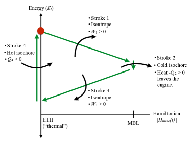
Figure 2: Otto engine cycle for a mesoscale MBL system: Two energies in the many-body spectrum capture the cycle’s basic physics. The engine can be regarded as beginning each trial in an energy eigenstate drawn from a Gibbs distribution. The red dot represents the engine’s starting state in some trial of interest. During stroke 1, $H_{\rm meso}(t)$ is tuned from “thermal” to MBL. During stroke 2, the engine thermalizes with a cold bath. $H_{\rm meso}(t)$ returns from MBL to thermal during stroke 3. Stroke 4 resets the engine, which thermalizes with a hot bath. The tunings (strokes 1 and 3) map onto the thermodynamic Otto cycle’s isentropes. The thermalizations (strokes 2 and 4) map onto isochores. The engine outputs work $W_{1}$ and $W_{3}$ during the tunings and absorbs heat $Q_{2}$ and $Q_{4}$ during thermalizations. MBL gap statistics’ lack of level repulsion enhances the cycle: The engine “slides down” the lines that represent tunings, losing energy outputted as work.

II A mesoscale MBL engine

We aim to formulate an MBL engine cycle for the thermodynamic limit. Our road to that goal runs through a finite-size, or mesoscale, MBL engine. In Sec. IIA, we introduce the intuition behind the mesoscale engine via a qubit toy model. Then, we describe (Sec. IIB) and quantitatively analyze (Sec. IIC) the mesoscale MBL engine. Table 1 offers a spotter’s guide to notation.

IIA Qubit toy model

At the MBL Otto engine’s core lies a qubit Otto engine whose energy eigenbasis transforms during the cycle Kosloff_02_Discrete ; Kieu_04_Second ; Kosloff_10_Optimal ; Cakmak_17_Irreversible . Consider a two-level system evolving under the time-varying Hamiltonian

$$H_{\rm qubit}(t):=(1-\alpha_{t})h\sigma^{x}+\alpha_{t}h^{\prime}\sigma^{z}\,.$$ (8)

$\sigma^{x}$and $\sigma^{z}$ denote the Pauli $x$- and $z$-operators. $\alpha_{t}$ denotes a parameter tuned between 0 and 1.

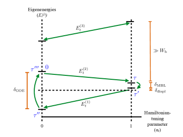
Figure 3: Qubit toy model for the MBL Otto cycle: A qubit models two “working levels” in the MBL Otto engine’s many-body spectrum. The energy eigenstates $\lvert E_{t}^{(1)}\rangle$ and $\lvert E_{t}^{(2)}\rangle$ span the “working subspace.” The gap $E_{t}^{(2)}-E_{t}^{(1)}$ begins at size $\delta_{\rm GOE}$ during a successful trial. The gap shrinks to $\delta_{\rm MBL}$, then returns to $\delta_{\rm GOE}$. In addition to changing the gap, each Hamiltonian tuning changes the eigenstates’ functional forms. The displacement $\delta_{\rm displ}$ is included for generality. The blue text marks the times $t=0,\tau,\ldots,\tau^{\prime\prime\prime}$ at which the strokes begin and end during a work-outputting trial. The spectator level $\lvert E_{t}^{(3)}\rangle$ fails to impact the engine’s efficiency. The cold bath has too narrow a bandwidth $W_{\rm b}$ to couple $\lvert E_{t}^{(3)}\rangle$ to any other level. If the engine begins any trial on the top green line, the engine remains on that line throughout the trial. Zero net work is outputted.

Figure 3 illustrates the cycle. The engine begins in thermal equilibrium at a high temperature $T_{\rm H}$. During stroke 1, the engine is thermally isolated, and $\alpha_{t}$ is tuned from 0 to 1. During stroke 2, the engine thermalizes to a temperature $T_{\rm C}\ll T_{\rm H}$. During stroke 3, the engine is thermally isolated, and $\alpha_{t}$ returns from 1 to 0. During stroke 4, the engine resets by thermalizing with the hot bath.

Let us make two simplifying assumptions (see (NYH_17_MBL, , App. C) for a generalization): First, let $T_{\rm H}=\infty$ and $T_{\rm C}=0$. Second, assume that the engine is tuned slowly enough to satisfy the quantum adiabatic theorem. We also choose

$$h=\frac{\delta_{\rm GOE}}{2}\,,\quad h^{\prime}=\frac{\delta_{\rm MBL}}{2}\,,$$

and $\delta_{\rm GOE}\gg\delta_{\rm MBL}$.

Let us analyze the cycle’s energetics. The system begins with $\left\langle H_{\rm qubit}(t)\right\rangle=0$. Stroke 1 preserves the infinite-temperature state $\mathbbm{1}/2$. The energy drops to $-\delta_{\rm MBL}/2$ during stroke 2 and to $-\delta_{\rm GOE}/2$ during stroke 3. During stroke 4, the engine resets to zero average energy, absorbing heat $\left\langle Q_{4}\right\rangle=\frac{\delta_{\rm GOE}}{2}$, on average.

The energy exchanged during the tunings (strokes 1 and 3) constitutes work [Eq. (6)], while the energy exchanged during the thermalizations (strokes 2 and 4) is heat [Eq. (7)]. The engine outputs the per-cycle power, or average work performed per cycle, $\left\langle W_{\rm tot}\right\rangle=\frac{1}{2}(\delta_{\rm GOE}-\delta_{\rm MBL})$.

The efficiency is $\eta_{\rm qubit}=\frac{\left\langle W_{\rm tot}\right\rangle}{\left\langle Q_{4}\right\rangle}=1-\frac{\delta_{\rm MBL}}{\delta_{\rm GOE}}$. This result is equivalent to the efficiency $\eta_{\rm Otto}$ of a thermodynamic Otto engine [Eq. (4)]. The gap ratio $\frac{\delta_{\rm MBL}}{\delta_{\rm GOE}}$ plays the role of $\frac{1}{r^{\gamma-1}}$. $\eta_{\rm qubit}$ equals also $\eta_{\rm QHO}$ [Eq. (5)] if the frequency ratio $\omega/\Omega$ is chosen to equal $\delta_{\rm MBL}/\delta_{\rm GOE}$. As shown in Sections II-III, however, the qubit engine can scale to a large composite engine of densely packed qubit subengines operating in parallel. The dense packing is possible if the qubits are encoded in the MBL system’s localized degrees of freedom (l-bits, roughly speaking Huse_14_phenomenology ).

IIB Set-up for the mesoscale MBL engine

Symbol	Significance
$N$	Number of sites per mesoscale engine (in Sec. II) or per mesoscale subengine
	(in the macroscopic engine, in Sec. III). Chosen, in the latter case, to equal $\xi_{>}$.
$\mathcal{N}$	Dimensionality of one mesoscale (sub)engine’s Hilbert space.
$\mathcal{E}$	Unit of energy, average energy density per site.
	Hamiltonian parameter tuned from 0 (in the mesoscale engine’s ETH regime,
$\alpha_{t}$	or the macroscopic engine’s shallowly localized regime)
	to 1 (in the engine’s deeply MBL regime).
$\left\langle\delta\right\rangle$	Average gap in the energy spectrum of a length-$N$ MBL system.
$W_{\rm b}$	Bandwidth of the cold bath. Small: $W_{\rm b}\ll\left\langle\delta\right\rangle$.
$\beta_{\rm H}=1/T_{\rm H}$	Inverse temperature of the hot bath.
$\beta_{\rm C}=1/T_{\rm C}$	Inverse temperature of the cold bath.
$\delta_{-}$	Level-repulsion scale of a length-$N$ MBL system. Minimal size reasonably attributable to
	any energy gap. Smallest gap size at which a Poissonian (1) approximates
	the MBL gap distribution well.
$v$	Speed at which the Hamiltonian is tuned: $v:=\mathcal{E}\frac{d\alpha_{t}}{t}$.
	Has dimensions of $1/\text{time}^{2}$, in accordance with part of DeGrandi_10_APT .
$\xi_{>}$	Localization length of macroscopic MBL engine when shallowly localized.
	Length of mesoscale subengine.
$\xi_{<}$	Localization length of macroscopic MBL engine when deeply localized. Satisfies $\xi_{<}<\xi_{>}$.
$X_{\rm macro}$	Characteristic $X$ of the macroscopic MBL engine (e.g., $X=N,\left\langle\delta\right\rangle$).
$g$	Strength of coupling between engine and cold bath.
$\tau_{\rm cycle}$	Time required to implement one cycle.
$\left\langle\delta\right\rangle^{(L)}$	Average energy gap of a length-$L$ MBL system.

Table 1: Parameters of the mesoscopic and macroscopic MBL engines: Introduced in Sections II and III. Boltzmann’s and Planck’s constants are set to one: $k_{\mathrm{B}}=\hbar=1$.

The next step is an interacting finite-size system tuned between MBL and ETH phases. Envision a mesoscale engine as a one-dimensional (1D) system of $N\approx 10$ sites. This engine will ultimately model one region in a thermodynamically large MBL engine. We will analyze the mesoscopic engine’s per-trial power $\left\langle W_{\rm tot}\right\rangle$, the efficiency $\eta_{\rm MBL}$, and work costs $\left\langle W_{\rm diab}\right\rangle$ of undesirable diabatic transitions.

The mesoscopic engine evolves under the Hamiltonian

$$H_{\rm meso}(t):=\frac{\mathcal{E}}{Q(\alpha_{t})}\left[(1-\alpha_{t})H_{\rm GOE}+\alpha_{t}\,H_{\rm MBL}\right]\,.$$ (9)

The unit of energy, or average energy density per site, is denoted by $\mathcal{E}$. The tuning parameter $\alpha_{t}\in[0,1]$. When $\alpha_{t}=0$, the system evolves under a random Hamiltonian $H_{\rm GOE}$ whose gaps $\delta$ are distributed according to $P^{(E)}_{\rm GOE}(\delta)$ [Eq. (2)]. When $\alpha_{t}=1$, $H_{\rm meso}(t)=H_{\rm MBL}$, a Hamiltonian whose gaps are distributed according to $P^{(E)}_{\rm MBL}(\delta)$ [Eq. (1)]. For a concrete example, take a random-field Heisenberg model whose disorder strength is tuned. $H_{\rm GOE}$ and $H_{\rm MBL}$ have the same bond term, but the disorder strength varies in time. We simulate (a rescaled version of) this model in Sec. V.

The mesoscale engine’s cycle is analogous to the qubit cycle, including initialization at $\alpha_{t}=0$, tuning of $\alpha_{t}$ to one, thermalization with a temperature-$T_{\rm C}$ bath, tuning of $\alpha_{t}$ to zero, and thermalization Huse_15_Localized ; DeLuca_15_Dynamic ; Levi_16_Robustness ; Fischer_16_Dynamics with a temperature-$T_{\rm H}$ bath. To highlight the role of level statistics in the cycle, we hold the average energy gap, $\left\langle\delta\right\rangle$, constant. We do so using the renormalization factor $Q(\alpha_{t})$. Section V details how we define $Q(\alpha_{t})$ in numerical simulations.

The key distinction between GOE level statistics (2) and Poisson (MBL) statistics (1) is that small gaps (and large gaps) appear more often in Poisson spectra. A toy model illuminates these level statistics’ physical origin: An MBL system can be modeled as a set of noninteracting quasilocal qubits Huse_14_phenomenology . Let $g_{j}$ denote the $j^{\rm th}$ qubit’s gap. Two qubits, $j$ and $j^{\prime}$, may have nearly equal gaps: $g_{j}\approx g_{j^{\prime}}$. The difference $|g_{j}-g_{j^{\prime}}|$ equals a gap in the many-body energy spectrum. Tuning the Hamiltonian from MBL to ETH couples the qubits together, producing matrix elements between the nearly degenerate states. These matrix elements force energies apart.

To take advantage of the phases’ distinct level statistics, we use a cold bath that has a small bandwidth $W_{\rm b}$. According to Sec. IIA, net positive work is extracted from the qubit engine because $\delta_{\rm MBL}<\delta_{\rm GOE}$. The mesoscale analog of $\delta_{\rm GOE}$ is $\sim\left\langle\delta\right\rangle$, the typical gap ascended during hot thermalization. The engine must not emit energy on this scale during cold thermalization. Limiting $W_{\rm b}$ ensures that cold thermalization relaxes the engine only across gaps $\delta\leq W_{\rm b}\ll\left\langle\delta\right\rangle$. Such anomalously small gaps appear more often in MBL energy spectra than in ETH spectra  Khaetskii_02_Electron ; Gopalakrishnan_14_Mean ; Parameswaran_17_Spin .

This level-statistics argument holds only within superselection sectors. Suppose, for example, that $H_{\rm meso}(t)$ conserves the particle number. The level-statistics arguments apply only if the particle number remains constant throughout the cycle (NYH_17_MBL, , App. F). Our numerical simulations (Sec. V) take place at half-filling, in a subspace of dimensionality $\mathcal{N}$ of the order of magnitude of the whole space’s dimensionality: $\mathcal{N}\sim\frac{2^{N}}{\sqrt{N}}$.

We are now ready to begin analyzing the mesoscopic-engine Otto cycle. The engine begins in the thermal state $\rho(0)=e^{-\beta_{\rm H}H_{\rm GOE}}/Z$, wherein $Z:={\rm Tr}\left(e^{-\beta_{\rm H}H_{\rm GOE}}\right)$. The engine can be regarded as starting each trial in some energy eigenstate $j$ drawn according to the Gibbs distribution (Fig. 2). During stroke 1, $H_{\rm meso}(t)$ is tuned from $H_{\rm GOE}$ to $H_{\rm MBL}$. We approximate the tuning as quantum-adiabatic (diabatic corrections are modeled in Sec. IV). Stroke 2, cold thermalization, depends on the gap $\delta^{\prime}_{j}$ between the $j^{\rm th}$ and $(j-1)^{\rm th}$ MBL levels. $\delta^{\prime}_{j}$ typically exceeds $W_{\rm b}$. If it does, cold thermalization preserves the engine’s energy, and the cycle outputs $W_{\rm tot}=0$. With probability $\sim\frac{W_{\rm b}}{\left\langle\delta\right\rangle}$, the gap is small enough to thermalize: $\delta^{\prime}_{j}<W_{\rm b}$. In this case, cold thermalization drops the engine to level $j-1$. Stroke 3 brings the engine to level $j-1$ of $H_{\rm GOE}$. The gap $\delta_{j}$ between the $(j-1)^{\rm th}$ and $j^{\rm th}$ $H_{\rm GOE}$ levels is $\left\langle\delta\right\rangle\gg W_{\rm b}$, with the high probability $\sim 1-(W_{\rm b}/\left\langle\delta\right\rangle)^{2}$. Hence the engine likely outputs $W_{\rm tot}>0$. Hot thermalization (stroke 4) returns the engine to $\rho(0)$.

IIC Quantitative analysis of the mesoscale engine in the adiabatic limit

How well does the mesoscale Otto engine perform? We calculate average work $\left\langle W_{\rm tot}\right\rangle$ outputted per cycle and the efficiency $\eta_{\rm MBL}$. Details appear in App. A.

We focus on the parameter regime in which the cold bath is very cold, the cold-bath bandwidth $W_{\rm b}$ is very small, and the hot bath is very hot: $T_{\rm C}\ll W_{\rm b}\ll\left\langle\delta\right\rangle$, and $\sqrt{N}\>\beta_{\rm H}\mathcal{E}\ll 1$. The mesoscale engine resembles a qubit engine whose state and gaps are averaged over. The gaps, $\delta_{j}$ and $\delta^{\prime}_{j}$, obey the distributions $P_{\rm GOE}^{(E)}(\delta_{j})$ and $P_{\rm MBL}^{(E)}(\delta^{\prime}_{j})$ [Eqs. (2) and (1)]. Correlations between the $H_{\rm GOE}$ and $H_{\rm MBL}$ spectra can be neglected.

We make three simplifying assumptions, generalizing later: (i) The engine is assumed to be tuned quantum-adiabatically. Diabatic corrections are estimated in Sec. IV. (ii) The hot bath is at $T_{\rm H}=\infty$. We neglect finite-temperature corrections, which scale as $N(\beta_{\rm H}\mathcal{E})^{2}\frac{(W_{\rm b})^{2}}{\left\langle\delta\right\rangle}$ and are calculated numerically in Suppl. Mat. A. (iii) The gap distributions vary negligibly with energy: $P_{\rm GOE}^{(E)}(\delta_{j})\approx P_{\rm GOE}(\delta_{j})$, and $P_{\rm MBL}^{(E)}(\delta^{\prime}_{j})\approx P_{\rm MBL}(\delta^{\prime}_{j})$, wherein $\left\langle\delta\right\rangle_{E}\approx\left\langle\delta\right\rangle$.

Average work $\left\langle W_{\rm tot}\right\rangle$ per cycle: The key is whether the cold bath relaxes the engine downwards across the MBL-side gap $\delta^{\prime}\equiv\delta^{\prime}_{j}$, distributed as $P_{\rm MBL}(\delta^{\prime})$, during a given trial. If $\delta^{\prime}<W_{\rm b}$, the engine has a probability $1/(1+e^{-\beta_{\rm C}\delta})$ of thermalizing. Hence the overall probability of relaxation by the cold bath is

$$p_{\rm cold}\approx\int\limits_{0}^{W_{\rm b}}d\delta^{\prime}\;\frac{1}{\left\langle\delta\right\rangle}\frac{e^{-\delta^{\prime}/\left\langle\delta\right\rangle}}{1+e^{-\beta_{\rm C}\delta^{\prime}}}\approx\frac{1}{\left\langle\delta\right\rangle}\left(W_{\rm b}-T_{C}\ln 2\right),$$ (11)

wherein we neglected $W_{\rm b}/\left\langle\delta\right\rangle$ by setting $e^{-\delta^{\prime}/\left\langle\delta\right\rangle}\approx 1$.

Alternatively, the cold bath could excite the engine to a level a distance $\delta^{\prime}$ above the initial level. Such an upward hop occurs with a probability

$$\bar{p}_{\rm cold}\approx\int\limits_{0}^{W_{\rm b}}d\delta^{\prime}\;\frac{e^{-\delta^{\prime}/\left\langle\delta\right\rangle}}{\left\langle\delta\right\rangle}\frac{e^{-\beta_{\rm C}\delta^{\prime}}}{1+e^{-\beta_{\rm C}\delta^{\prime}}}\approx\frac{T_{C}\ln 2}{\left\langle\delta\right\rangle}\,.$$ (12)

If the engine relaxed downward during stroke 2, then upon thermalizing with the hot bath during stroke 4, the engine gains heat $\left\langle Q\right\rangle_{4}\approx\left\langle\delta\right\rangle$, on average. If the engine thermalized upward during stroke 2, then the engine loses $\left\langle\delta\right\rangle$ during stroke 4, on average. Therefore, the cycle outputs average work

$$\left\langle W_{\rm tot}\right\rangle\approx\left(p_{\rm cold}-\bar{p}_{\rm cold}\right)\left\langle\delta\right\rangle+\left\langle Q_{2}\right\rangle\approx W_{\rm b}-\frac{2\ln 2}{\beta_{\rm C}}\,.$$ (13)

$\left\langle Q_{2}\right\rangle$ denotes the average heat absorbed by the engine during cold thermalization:

$$\left\langle Q_{2}\right\rangle\approx-\int\limits_{0}^{W_{\rm b}}d\delta^{\prime}\;\frac{\delta^{\prime}}{\left\langle\delta\right\rangle}\frac{e^{-\delta^{\prime}/\left\langle\delta\right\rangle}}{1+e^{-\beta_{\rm C}\delta^{\prime}}}\approx-\frac{(W_{\rm b})^{2}}{2\left\langle\delta\right\rangle}\,,$$ (14)

which is $\ll\left\langle Q_{4}\right\rangle$. This per-cycle power scales with the system size $N$ as $W_{\rm b}\ll\left\langle\delta\right\rangle\sim\frac{\text{effective bandwidth}}{\text{\# energy eigenstates}}\sim\frac{\mathcal{E}\sqrt{N}}{\mathcal{N}}$.

Efficiency $\eta_{\rm MBL}$: The efficiency is

$$\eta_{\rm MBL}=\frac{\left\langle W_{\rm tot}\right\rangle}{\left\langle Q_{4}\right\rangle}=\frac{\left\langle Q_{4}\right\rangle+\left\langle Q_{2}\right\rangle}{\left\langle Q_{4}\right\rangle}\approx 1-\frac{W_{\rm b}}{2\left\langle\delta\right\rangle}\,.$$ (15)

The imperfection is small, $\frac{W_{\rm b}}{2\left\langle\delta\right\rangle}\ll 1$, because the cold bath has a small bandwidth. This result mirrors the qubit-engine efficiency $\eta_{\rm qubit}$. But our engine is a many-body system of $N$ interacting sites. MBL will allow us to employ segments of the system as independent qubit-like subengines, despite interactions. In the absence of MBL, each subengine’s effective $\left\langle\delta\right\rangle=0$. With $\left\langle\delta\right\rangle$ vanishes the ability to extract $\left\langle W_{\rm tot}\right\rangle>0$. Whereas the efficiency is nearly perfect, an effective engine requires also a finite power. The MBL engine’s power will depend on dynamics, as discussed below.

III MBL engine in the thermodynamic limit

The MBL engine’s advantage lies in having a simple thermodynamic limit that does not compromise efficiency or power output. A nonlocalized Otto engine would suffer from a suppression of the average level spacing: $\left\langle\delta\right\rangle\sim\frac{\mathcal{E}\sqrt{N}}{2^{N}}$, which suppresses the average output per cycle, $\left\langle W_{\rm tot}\right\rangle\sim W_{\rm b}\ll\left\langle\delta\right\rangle$, exponentially in the system size. Additionally, the tuning speed $v$ must shrink exponentially: $H_{\rm meso}(t)$ is ideally tuned quantum-adiabatically. The time per tuning stroke must far exceed $\left\langle\delta\right\rangle^{-1}$. The mesoscale engine scales poorly, but properties of MBL offer a solution.

A thermodynamically large MBL Otto engine consists of mesoscale subengines that operate mostly independently. This independence hinges on local level correlations of the MBL phase Sivan_87_Energy ; imryma ; Syzranov_17_OTOCs : Subsystems separated by a distance $L$ evolve roughly independently until times exponential in $L$, due to the localization Nandkishore_15_MBL .

Particularly important is the scaling of the typical strength of a local operator in an MBL phase. Let $O$ denote a generic local operator that has support on just a size-$L$ region. $O$ can connect only energy eigenstates $\lvert\psi_{1}\rangle$ and $\lvert\psi_{2}\rangle$ that differ just in their local integrals of motion in that region. Such states are said to be “close together,” or “a distance $L$ apart .” Let $\xi$ denote the system’s localization length. If the eigenfunctions lie far apart ($L\gtrsim\xi$), the matrix-element size scales as

$$|O_{21}|\sim 2^{-L}e^{-L/\xi}\,.$$ (16)

(All lengths appear in units of the lattice spacing, set to one.) This scaling determines the typical level spacing, since such matrix elements give rise to level repulsion:

$$\delta\sim\mathcal{E}2^{-L}e^{-L/\xi}\,$$ (17)

(possibly to within a power-law correction). The localization-induced exponential suppresses long-distance communication (see Anderson_58_Absence ; Sivan_87_Energy ; BAA ; Nandkishore_15_MBL and App. B).

Let us apply this principle to a chain of $N$-site mesoscale engines separated by $N$-site buffers. The engine is cycled between a shallowly localized ($H_{\rm GOE}$-like) Hamiltonian, which has a localization length $\xi_{>}$, and a deeply localized ($H_{\rm MBL}$-like) Hamiltonian, which has $\xi_{<}\ll\xi_{>}$.

The key element in the construction is that the cold bath acts through local operators confined to $<N\sim\xi_{>}$ sites. This defines the subengines of the thermodynamic MBL Otto engine. Localization guarantees that “what happens in a subengine stays in a subengine”: Subengines do not interfere much with each other’s operation.

This subdivision boosts the engine’s power. A length-$N$ mesoscale engine operates at the average per-cycle power $\left\langle W_{\rm tot}\right\rangle_{\rm meso}\sim W_{\rm b}\ll\frac{\mathcal{E}\sqrt{N}}{2^{N}}$ (Sec. IIC). A subdivided length-$N_{\rm macro}$ MBL engine outputs average work $\sim\frac{N_{\rm macro}}{2N}\left\langle W_{\rm tot}\right\rangle_{\rm meso}$. In contrast, if the length-$N_{\rm macro}$ engine were not subdivided, it would output average work $\sim\frac{\mathcal{E}\sqrt{N_{\rm macro}}}{2^{N_{\rm macro}}}$, which vanishes in the thermodynamic limit.

IV Time-scale restrictions on the MBL Otto engine’s operation

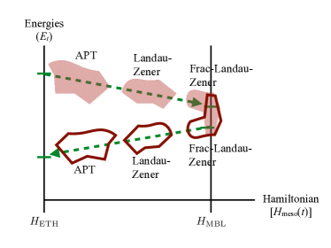
Figure 4: Three (times two) classes of diabatic transitions: Hops to arbitrary energy levels, modeled with general adiabatic perturbation theory (APT), plague the ETH regime. Landau-Zener transitions and fractional-Landau-Zener transitions plague the many-body-localized regime.

We estimate the restrictions on the speed with which the Hamiltonian must be tuned to avoid undesirable diabatic transitions and intersubengine communication. Most importantly, we estimate the time required for cold thermalization (stroke 2).

IVA Diabatic corrections

We have modeled the Hamiltonian tuning as quantum-adiabatic, but realistic tuning speeds $v:=\mathcal{E}\left\lvert\frac{d\alpha_{t}}{dt}\right\rvert$ are finite. To understand diabatic tuning’s effects, we distinguish the time-$t$ density matrix $\rho(t)$ from the corresponding diagonal ensemble,

$$\begin{split}&\rho_{\mathrm{diag}}(t)=\sum_{j}\lvert E_{j}(t)\rangle\varepsilon_{j}(t)\langle E_{j}(t)\rvert\,,\quad\text{wherein}\\ &\varepsilon_{j}(t)=\langle E_{j}(t)\rvert\rho\lvert E_{j}(t)\rangle\end{split}$$ (18)

and $\lvert E_{j}(t)\rangle$ denotes an instantaneous energy eigenbasis of $H_{{\rm meso}}(t)=\sum_{j}\lvert E_{j}(t)\rangle E_{j}(t)\langle E_{j}(t)\rvert$. The average energy depends on $\rho(t)$ only through $\rho_{\mathrm{diag}}(t)$. [More generally, the state’s off-diagonal elements dephase under the dynamics. $\rho_{\rm diag}(t)$ is “slow” and captures most of the relevant physics D'Alessio_16_From .]

In the adiabatic limit, $\varepsilon_{j}(t)=\varepsilon_{j}(0)$. We seek to understand how this statement breaks down when the tuning proceeds at a finite speed $v$. It is useful to think of “infinite-temperature thermalization” in the sense of this diagonal ensemble: Fast tuning may push the diagonal-ensemble weights $\varepsilon_{j}(t)$ towards uniformity—even though the process is unitary and the entropy $S=-\rho(t)\ln\rho(t)$ remains constant—thanks to the off-diagonal elements.

The effects of diabatic tuning appear in three distinct regimes, which we label “fractional-Landau-Zener,” “Landau-Zener,” and “APT” (Fig. 4). We estimate the average per-cycle work costs $\left\langle W_{\rm diab}\right\rangle$ of diabatic jumps, guided by the numerics in Sec. V. We focus on $T_{\rm H}=\infty$ and $T_{\rm C}=0$, for simplicity. Since $T_{\rm H}=\infty$, diabatic hops cannot bring $\rho_{\rm diag}(t)$ closer to $\mathbbm{1}/2^{N}$—cannot change the average energy—during stroke 1. Hence we focus on stroke 3.

IVA1 Fractional-Landau-Zener transitions

At the beginning of stroke 3, nonequilbrium effects could excite the system back across the small gap to energy level $j$. The transition would cost work and would prevent the trial from outputting $W_{\rm tot}>0$. We dub this excitation a fractional-Landau-Zener (frac-LZ) transition. It could be suppressed by a sufficiently slow drive DeGrandi_10_APT . The effects, and the resultant bound on $v$, are simple to derive.

Let the gap start stroke 3 at size $\delta$ and grow to a size $\Delta>\delta$. Because the two energy levels begin close together, one cannot straightforwardly apply the Landau-Zener formula. One must use the fractional-Landau-Zener result of De Grandi and Polkovnikov DeGrandi_10_APT ,

$$p_{\text{frac-LZ}}(\delta)\approx\frac{v^{2}(\delta_{-})^{2}}{16}\left(\frac{1}{\delta^{6}}+\frac{1}{\Delta^{6}}\right)\approx\frac{v^{2}(\delta_{-})^{2}}{16\delta^{6}}\,.$$ (19)

$\delta_{-}$ denotes the MBL level-repulsion scale, the characteristic matrix element introduced by a perturbation between eigenstates of an unperturbed Hamiltonian. We suppose that energy-level pairs with $p_{\text{frac-LZ}}\lesssim 1$ are returned to the infinite-temperature state from which the cold bath disturbed them. These pairs do not contribute to $\left\langle W_{\rm tot}\right\rangle$. Pairs that contribute have $p_{\text{frac-LZ}}<1$, i.e.,

$$\delta>(v\delta_{-})^{1/3}\,.$$ (20)

If the rest of the stroke is adiabatic, the average work performed during the cycle is

$$\left\langle W_{\rm tot}\right\rangle\sim\left\langle Q_{4}\right\rangle-\left\langle Q_{2}\right\rangle-(v\delta_{-})^{1/3}\,,$$ (21)

which results immediately in the correction

$$\left\langle W_{\mathrm{diab},\text{frac-LZ}}\right\rangle\sim(v\delta_{-})^{1/3}\,.$$ (22)

This correction is negligible at speeds low enough that

$$v\ll\frac{(W_{\rm b})^{3}}{\delta_{-}}\,.$$ (23)

IVA2 Landau-Zener transitions

While the system is localized, the disturbances induced by the tuning $\frac{dH(t)}{dt}$ can propagate only a short distance $l_{v}$. The tuning effectively reduces the mesoscale engine to a length-$l_{v}$ subengine. To estimate $l_{v}$, we compare the minimum gap of a length-$l_{v}$ subsystem to the speed $v$:

$$\mathcal{E}2^{-l_{v}}e^{-l_{v}/\xi_{<}}\sim\sqrt{v}\;.$$ (24)

The left-hand side comes from Eq. (17). This minimum gap—the closest that two levels are likely to approach—is given by the smallest level-repulsion scale, $\delta_{-}$. $\delta_{-}$ characterizes the deeply localized system, whose $\xi=\xi_{<}$. Consequently,

$$l_{v}\sim\frac{\ln(\mathcal{E}^{2}/v)}{2\Big{(}\ln 2+\frac{1}{\xi}_{<}\Big{)}}\,.$$ (25)

Suppose that $l_{v}\leq N$, and consider a length-$l_{v}$ effective subengine. In the adiabatic limit, $\left\langle W_{\rm tot}\right\rangle$ does not depend on the engine’s size. ($\left\langle W_{\rm tot}\right\rangle$ depends only on the bath bandwidth $W_{\rm b}\ll\left\langle\delta\right\rangle$.) To estimate how a finite $v$ changes $\left\langle W_{\rm tot}\right\rangle$, we consider the gaps $\delta<W_{\rm b}$ of the size-$l_{v}$ subengine. We divide the gaps into two classes:

1. Gaps connected by flipping l-bits on a region of diameter $l<l_{v}$. The tuning is adiabatic with respect to these gaps, so they result in work output.

2. Gaps connected by flipping l-bits on a region of diameter $l=l_{v}$. The tuning is resonant with these gaps and so thermalizes them, in the sense of the diagonal ensemble [Eq. (18)]: The tuning makes the instantaneous-energy-eigenvector weights $\varepsilon_{j}$ uniform, on average.

Type-1 gaps form a $v$-independent $O(1)$ fraction $\theta$ of the length-$l_{v}$ subengine’s short-length-scale gaps. Type-2 gaps therefore make up a fraction $1-\theta$. Hence Landau-Zener physics leads to a $v$-independent $O(1)$ diabatic correction $(1-\theta)W_{\rm b}$ to $\left\langle W_{\rm tot}\right\rangle$, provided that $v$ is high enough that $l_{v}<N$.

IVA3 Adiabatic-perturbation-theory (APT) transitions

When the system is in the ETH phase (or has correlation length $\xi\sim N$), typical minimum gaps (points of closest approach) are still given by the level-repulsion scale, which is now $\left\langle\delta\right\rangle$. Hence one expects the tuning to be adiabatic if

$$v\ll\left\langle\delta\right\rangle^{2}\,.$$ (26)

This criterion could be as stringent (depending on the system size and localization lengths) as the requirement (23) that fractional Landau-Zener transitions occur rarely. The numerics in Sec. VC indicate that fractional-Landau-Zener transitions limit the power more than APT transitions do.

Both fractional Landau-Zener transitions and APT transitions bound the cycle time $\tau_{\rm cycle}$ less stringently than thermalization with the cold bath; hence a more detailed analysis of APT transitions would be gratuitous. Such an analysis would rely on the general adiabatic perturbation theory of De Grandi and Polkovnikov DeGrandi_10_APT ; hence the moniker “APT transitions.”

IVB Precluding communication between subengines

To maintain the MBL engine’s advantage, we must approximately isolate subengines. The subengines’ (near) independence implies a lower bound on the tuning speed $v$: The price paid for scalability is the impossibility of adiabaticity. Suppose that $H_{\rm macro}(t)$ were tuned infinitely slowly. Information would have time to propagate from one subengine to every other. The slow spread of information through MBL Khemani_15_NPhys_Nonlocal lower-bounds $v$. This consideration, however, does not turn out to be the most restrictive constraint on the cycle time. Therefore, we address it only qualitatively.

As explained in Sec. IVA2, $v$ determines the effective size of an MBL subengine. Ideally, $v$ is large enough to prevent adiabatic transitions between configurations extended beyond the mesoscale $N$. For each stage of the engine’s operation, $v$ should exceed the speed given in Eq. (24) for the localization length $\xi$ of a length-$(N+1)$ chain:

$$v\gg[\delta_{-}(N+1,\xi)]^{2}\sim\mathcal{E}^{2}2^{-2(N+1)}e^{-2(N+1)/\xi}.$$ (27)

(We have made explicit the dependence of the level-repulsion scale $\delta_{-}$ on the mesoscale-engine size $N$ and on the localization length $\xi$.) During stroke 1, $\xi$ drops, so the RHS of (27) decays quickly. Hence the speed should interpolate between $[\delta_{-}(N+1,\xi_{>})]^{2}$ and $\frac{(W_{\rm b})^{3}}{\delta_{-}(N,\xi_{<})}$ [from Ineq. (23)].

IVC Lower bound on the cycle time $\tau_{\rm cycle}$ from cold thermalization:

Thermalization with the cold bath (stroke 2) bounds $\tau_{\rm cycle}$ more stringently than the Hamiltonian tunings do. The reasons are (i) the slowness with which MBL thermalizes and (ii) the restriction $W_{\rm b}\ll\left\langle\delta\right\rangle$ on the cold-bath bandwidth. We elaborate after introducing our cold-thermalization model (see (NYH_17_MBL, , App. I) for details).

We envision the cold bath as a bosonic system that couples to the engine locally, as via the Hamiltonian

$$H_{\rm int} =g\int_{-W_{\rm b}/\xi_{>}}^{W_{\rm b}/\xi_{>}}d\omega\sum_{j\in{\rm subengine}}\left(c_{j}^{\dagger}c_{j+1}+{\rm h.c.}\right)\left(b_{\omega}+b_{\omega}^{\dagger}\right)$$

$$\qquad\times\delta\bm{(}\langle 0|c_{j}H_{\rm macro}(\tau)c_{j+1}^{\dagger}|0\rangle-\omega\bm{)}\,.$$ (28)

The sum runs over the sites in the subengines, excluding the sites in the buffers between subengines. The coupling strength is denoted by $g$. We have switched from spin notation to fermion notation via a Jordan-Wigner transformation. $c_{j}$ and $c_{j}^{\dagger}$ denote the annihilation and creation of a fermion at site $j$. $H_{\rm macro}(t)$ denotes the Hamiltonian that would govern the engine at time $t$ in the bath’s absence. Cold thermalization lasts from $t=\tau$ to $t=\tau^{\prime}$ (Fig. 3). $b_{\omega}$ and $b_{\omega}^{\dagger}$ represent the annihilation and creation of a frequency-$\omega$ boson in the bath. The Dirac delta function is denoted by $\delta(.)$.

The bath couples locally, e.g., to pairs of nearest-neighbor spins. This locality prevents subengines from interacting with each other much through the bath. The bath can, e.g., flip spin $j$ upward while flipping spin $j+1$ downward. These flips likely change a subengine’s energy by an amount $E$. The bath can effectively absorb only energy quanta of size $\leq W_{\rm b}$ from any subengine. The cap is set by the bath’s speed of sound KimPRL13 , which follows from microscopic parameters in the bath’s Hamiltonian Lieb_72_Finite . The rest of the energy emitted during the spin flips, $|E-W_{\rm b}|$, is distributed across the subengine as the intrinsic subengine Hamiltonian flips more spins.

Let $\tau_{\rm th}$ denote the time required for stroke 2. We estimate $\tau_{\rm th}$ from Fermi’s Golden Rule,

$$\Gamma_{fi}=\frac{2\pi}{\hbar}|\langle f|V|i\rangle|^{2}\,\mu_{\rm bath}\,.$$ (29)

Cold thermalization transitions the engine from an energy level $\lvert i\rangle$ to a level $\lvert f\rangle$. The bath has a density of states $\mu_{\rm bath}\sim 1/W_{\rm b}$. $V$ denotes the operator, defined on the engine’s Hilbert space, induced by the coupling to the bath.

We estimate the matrix-element size $|\langle f|V|i\rangle|$ as follows. Cold thermalization transfers energy $E_{if}\sim W_{\rm b}$ from the subengine to the bath. $W_{\rm b}$ is very small. Hence the energy change rearranges particles across a large distance $L\gg\xi=\xi_{<}$, due to local level correlations (17). $V$ nontrivially transforms just a few subengine sites. Such a local operator rearranges particles across a large distance $L$ at a rate that scales as (17), $\mathcal{E}e^{-L/\xi}\;2^{-L}\sim\delta_{-}$. Whereas $\mathcal{E}$ sets the scale of the level repulsion $\delta_{-}$, $g$ sets the scale of $|\langle f|V|i\rangle|$. The correlation length $\xi=\xi_{<}$ during cold thermalization. We approximate $L$ with the subengine length $\xi_{>}$. Hence $|\langle f|V|i\rangle|\sim\frac{g\delta_{-}}{\mathcal{E}}$.

We substitute into Eq. (29). The transition rate $\Gamma_{fi}=\frac{1}{\tau_{\rm th}}$. Inverting yields

$$\tau_{\rm cycle}\sim\tau_{\rm th}\sim W_{\rm b}\left(\frac{\mathcal{E}}{g\delta_{-}}\right)^{2}\,.$$ (30)

To bound $\tau_{\rm cycle}$, we must bound the coupling $g$. The interaction is assumed to be Markovian: Information leaked from the engine dissipates throughout the bath quickly. Bath correlation functions must decay much more quickly than the coupling transfers energy. If $\tau_{\rm bath}$ denotes the correlation-decay time, $\tau_{\rm bath}<\frac{1}{g}$. The small-bandwidth bath’s $\tau_{\rm bath}\sim 1/W_{\rm b}$, so $g<W_{\rm b}$. This inequality, with Ineq. (30), implies

$$\tau_{\rm cycle}=\tau_{\rm th}>\frac{\mathcal{E}^{2}}{W_{\rm b}(\delta_{-})^{2}}\sim\frac{10}{\mathcal{E}}\>e^{2\xi_{>}/\xi_{<}}\>2^{3\xi_{>}}\,.$$ (31)

The final expression follows if $W_{\rm b}\sim\frac{\left\langle\delta\right\rangle}{10}$.

Like Markovianity, higher-order processes bound $\tau_{\rm th}$. Such processes transfer energy $E>W_{\rm b}$ between the engine and the cold bath. These transfers must be suppressed. $g^{a}$, wherein $a>1$, determine the rates at which these processes occur. The resulting bound on $\tau_{\rm th}$ is less stringent than Ineq. (31) (App. C).

V Numerical simulations

We use numerical exact diagonalization to check our analytical results. In Sec. VA, we describe the Hamiltonian used in our numerics. In Sec. VB, we study engine performance in the adiabatic limit (addressed analytically in Sec. IIC). In Sec. VC, we study diabatic corrections (addressed analytically in Sec. IVA). We numerically study the preclusion of communication between mesoscale subengines (addressed analytically in Sec. IVB) only insofar as these results follow from diabatic corrections: Limitations on computational power restricted the system size to 12 sites. Details about the simulation appear in App. D. Our code is available at https://github.com/christopherdavidwhite/MBL-mobile.

VA Hamiltonian

The engine can be implemented with a disordered Heisenberg model. A similar model’s MBL phase has been realized with ultracold atoms Schreiber_15_Observation . We numerically simulated a 1D mesoscale chain governed by a Hamiltonian

$$H_{\rm sim}(t)=\frac{\mathcal{E}}{Q\bm{(}h(\alpha_{t})\bm{)}}\Bigg{[}\sum_{j=1}^{N-1}\bm{\sigma}_{j}\cdot\bm{\sigma}_{j+1}+h(\alpha_{t})\sum_{j=1}^{N}h_{j}\sigma_{j}^{z}\Bigg{]}\,;$$ (32)

this is a special case of the general mesoscopic Hamiltonian (9) described in Sec. IIB. Equation (32) describes spins equivalent to interacting spinless fermions. Energies are expressed in units of $\mathcal{E}$, the average per-site energy density. For $\gamma=x,y,z$, the $\gamma^{\rm th}$ Pauli operator that operates nontrivially on the $j^{\rm th}$ site is denoted by $\sigma_{j}^{\gamma}$. The Heisenberg interaction $\bm{\sigma}_{j}\cdot\bm{\sigma}_{j+1}$ encodes nearest-neighbor hopping and repulsion.

The tuning parameter $\alpha_{t}\in[0,1]$ determines the phase occupied by $H_{\rm sim}(t)$. The site-$j$ disorder potential depends on a random variable $h_{j}$ distributed uniformly across $[-1,1].$ The disorder strength $h(\alpha_{t})$ varies as $h(\alpha_{t})=\alpha_{t}\,h_{\rm GOE}+(1-\alpha_{t})h_{\rm MBL}$. When $\alpha_{t}=0$, the disorder is weak, $h=h_{\rm GOE}$, and the engine occupies the ETH phase. When $\alpha_{t}=1$, the disorder is strong, $h=h_{\rm MBL}\gg h_{\rm GOE}$, and the engine occupies the MBL phase.

The normalization factor $Q\bm{(}h(\alpha_{t})\bm{)}$ preserves the width of the density of states (DOS) and so preserves $\left\langle\delta\right\rangle$. $Q\bm{(}h(\alpha_{t})\bm{)}$ prevents the work extractable via change of bandwidth from polluting the work extracted with help from level statistics (see App. E 1 for a discussion of work extraction from bandwidth change). $Q\bm{(}h(\alpha_{t})\bm{)}$ is defined and calculated in App. D 1.

The ETH-side field had a magnitude $h(0)=2.0$, and the MBL-side field had a magnitude $h(1)=20.0$. These $h(\alpha_{t})$ values fall squarely on opposite sides of the MBL transition at $h\approx 7$.

VB Adiabatic engine

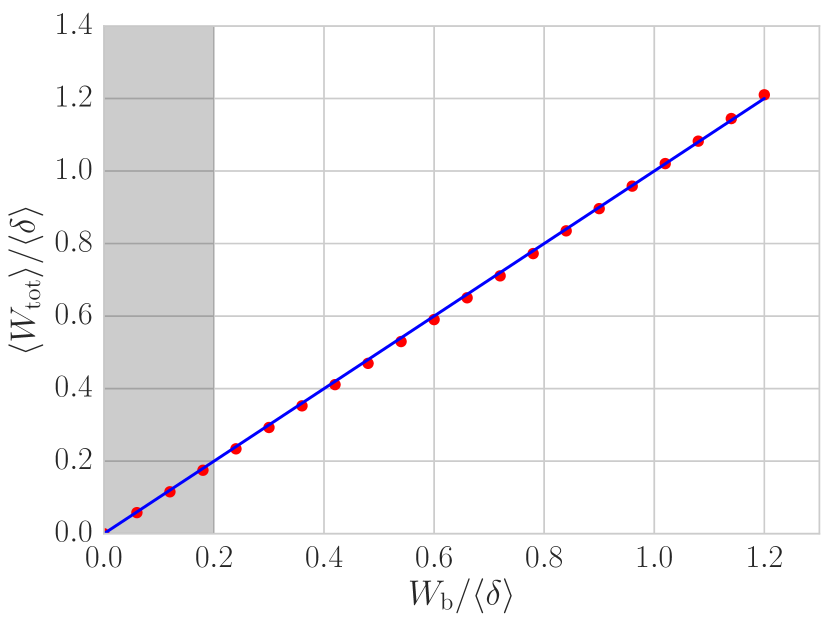
(a)

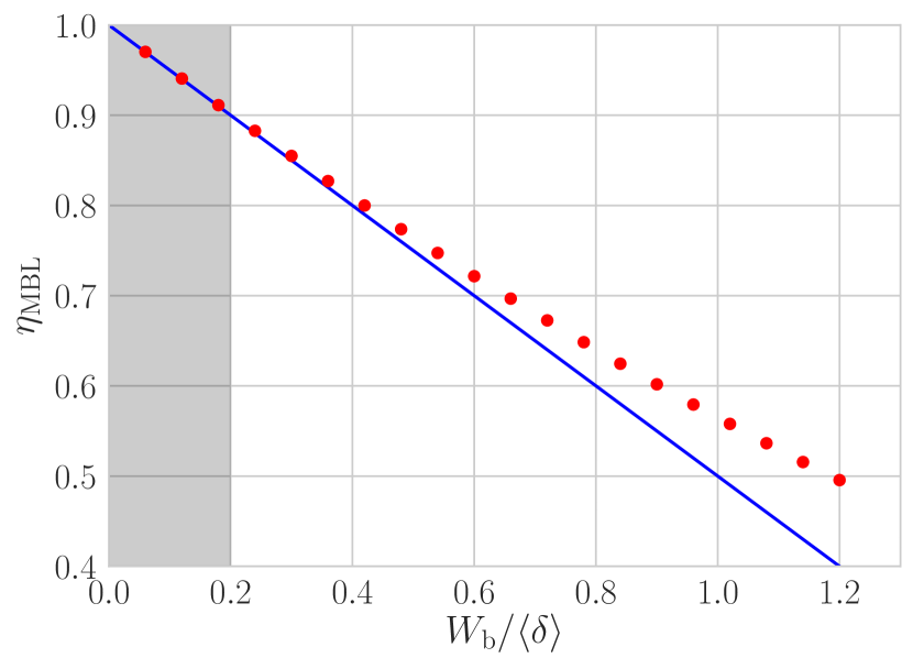
(b)

Figure 5: Average per-cycle power $\left\langle W_{\rm tot}\right\rangle$ (top) and efficiency $\eta_{\rm MBL}$ (bottom) as functions of the cold-bath bandwidth $W_{\rm b}$: Each red dot represents an average over 1,000 disorder realizations of the random-field Heisenberg Hamiltonian (32). The blue lines represent the analytical predictions (13) and (15) of Sec. IIC. When $W_{\rm b}\ll\left\langle\delta\right\rangle$ (in the gray shaded region), the engine operates in the regime of interest. Here, $\left\langle W_{\rm tot}\right\rangle$ and $\eta_{\rm MBL}$ vary linearly with $W_{\rm b}$, as predicted. The error bars are smaller than the numerical-data points.

We compare the analytical predictions of of Sec. IIC and App. A to numerical simulations of a 12-site engine governed by the Hamiltonian (32). During strokes 1 and 3, the state was evolved as though the Hamiltonian were tuned adiabatically. We index the energies $E_{j}(t)$ from least to greatest at each instant: $E_{j}(t)<E_{k}(t)\;\forall j<k$. Let $\rho_{j}$ denote the state’s weight on eigenstate $j$ of the initial Hamiltonian, whose $\alpha_{t}=0$. The engine ends stroke 1 with weight $\rho_{j}$ on eigenstate $j$ of the post-tuning Hamiltonian, whose $\alpha_{t}=1$.

The main results appear in Fig. 5. Figure 5(a) shows the average work extracted per cycle, $\left\langle W_{\rm tot}\right\rangle$. Figure 5(b) shows the efficiency, $\eta_{\rm MBL}$.

In these simulations, the baths had the extreme temperatures $T_{\rm H}=\infty$ and $T_{\rm C}=0$. This limiting case elucidates the $W_{\rm b}$-dependence of $\left\langle W_{\rm tot}\right\rangle$ and of $\eta_{\rm MBL}$: Disregarding finite-temperature corrections, on a first pass, builds intuition. Finite-temperature numerics appear alongside finite-temperature analytical calculations in App. A.

Figure 5 shows how the per-cycle power and the efficiency depend on the cold-bath bandwidth $W_{\rm b}$. As expected, $\left\langle W_{\rm tot}\right\rangle\approx W_{\rm b}$. The dependence’s linearity, and the unit proportionality factor, agree with Eq. (13). Also as expected, the efficiency declines as the cold-bath bandwidth rises: $\eta_{\rm MBL}\approx 1-\frac{W_{\rm b}}{2\left\langle\delta\right\rangle}\,.$ The linear dependence and the proportionality factor agree with Eq. (15).

The gray columns in Fig. 5 highlight the regime in which the analytics were performed, where $\frac{W_{\rm b}}{\left\langle\delta\right\rangle}\ll 1$. If the cold-bath bandwidth is small, $W_{\rm b}<\left\langle\delta\right\rangle$, the analytics-numerics agreement is close. But the numerics agree with the analytics even outside this regime. If $W_{\rm b}\gtrsim\left\langle\delta\right\rangle$, the analytics slightly underestimate $\eta_{\rm MBL}$: The simulated engine operates more efficiently than predicted. To predict the numerics’ overachievement, one would calculate higher-order corrections in App. A: One would Taylor-approximate to higher powers, modeling subleading physical processes. Such processes include the engine’s dropping across a chain of three small gaps, $\delta^{\prime}_{1}\,,\delta^{\prime}_{2}\,,\delta^{\prime}_{3}<W_{\rm b}$, during cold thermalization.

The error bars are smaller than the numerical-data points. Each error bar represents the error in the estimate of a mean (of $\left\langle W_{\rm tot}\right\rangle$ or of $\eta_{\rm MBL}:=1-\frac{\left\langle W_{\rm tot}\right\rangle}{\left\langle Q_{\rm in}\right\rangle}$) over 1,000 disorder realizations. Each error bar extends a distance $(\text{sample standard deviation})/\sqrt{\text{\# realizations}}$ above and below that mean.

VC Diabatic engine

We then simulated strokes 1 and 3 as though $H_{\rm sim}(t)$ were tuned at finite speed $v$. Computational limitations restricted the engine to 8 sites. (That our upper bounds on $v$ scale as powers of $\left\langle\delta\right\rangle\sim 2^{-N}$ implies that these simulations quickly become slow to run.) We simulate a stepwise tuning, taking

$$\alpha_{t}=\frac{\delta t\,\lfloor t/\delta t\rfloor}{T}\,.$$ (33)

$\delta t$ denotes a time-step size, and $T\propto\frac{h_{\rm MBL}-h_{\mathrm{GOE}}}{v}$ denotes the time for which one tuning stroke lasts. This protocol is more violent than the protocols treated analytically: $v$ is assumed to remain finite in the diabatic analytics. In the numerics, we tune by sudden jumps (for reasons of numerical convenience). We work at $T_{\rm H}=\infty$ and $T_{\rm C}=0$—again, to capture the essential physics without the complication of finite-temperature corrections.

Figure 6 shows the average work output, $\left\langle W_{\rm tot}\right\rangle$, as a function of $v$. Despite the simulated protocol’s violence, both a fractional-Landau-Zener correction $W_{\text{frac-LZ}}\sim(v\delta_{-})^{3}$, explained in Sec. IVA1, and a $v$-independent $O(1)$ Landau-Zener correction, explained in Sec. IVA2, are visible. We believe that the adiabatic numerics ($v=0$ red dot) differ from the analytics (blue line) due to finite-size effects: For small systems away from the spectrum’s center, the average gap estimated from the density of states can vary appreciably over one gap. These numerics confirm the analytics and signal the MBL Otto engine’s robustness with respect to changes in the tuning protocol.

Figure 6: Average per-cycle work as a function of tuning speed: We numerically simulated 995 disorder realizations of the random-field Heisenberg Hamiltonian (32) for a system of $N=8$ sites (red dots). The results are compared to the analytical estimate (13) for the adiabatic work output (blue line) and an empirical straight-line fit $W_{\rm tot}=W_{0}-W_{1}(v\delta_{-})^{1/3}/W_{\rm b}$ (black line). Errors in the estimate of the mean, computed as $(\text{sample standard deviation})/\sqrt{(}\#\ \text{realizations})$, lead to error bars smaller than the numerical-data points.

VI Order-of-magnitude estimates

How well does the localized engine perform? We estimate the engine’s power and power density, in addition to comparing the engine with three competitors.

Localized engine: Localization has been achieved in solid-state systems. Consider silicon doped with phosphorus Kramer_93_Localization . A distance of $\sim 10\text{ nm}$ may separate phosphorus impurities. Let our engine cycle’s shallowly localized regime have a localization length of $\xi_{>}\sim 10$ sites, or $100\text{ nm}$. The work-outputting degrees of freedom will be electronic. The localized states will correspond to energies $\mathcal{E}\sim 1\text{ eV}$. Each subengine’s half-filling Hilbert space has dimensionality $\mathcal{N}={10\choose 5}\sim 10^{2}$. Hence each subengine has an effective average gap $\left\langle\delta\right\rangle\sim\frac{\mathcal{E}\sqrt{N}}{\mathcal{N}}\sim\frac{1\text{ eV}}{10^{2}}\sim 10\text{ meV}$. The cold-bath bandwidth must satisfy $\left\langle\delta\right\rangle\gg W_{\rm b}\,.$ We set $W_{\rm b}$ to be an order of magnitude down from $\left\langle\delta\right\rangle$: $W_{\rm b}\sim 1\text{ meV}\sim 10\text{ K}$. The cold-bath bandwidth approximates the work outputted by one subengine per cycle: $\left\langle W_{\rm tot}\right\rangle\sim W_{\rm b}\sim 1\text{ meV}$ [Eq. (13)].

What volume does a localized subengine fill? Suppose that the engine is three-dimensional (3D). A little room should separate the subengines. Classical-control equipment requires more room. Also, the subengine needs space to connect to the baths. We therefore associate each subengine with a volume of $V\approx(100\text{ nm})^{3}$.

The last element needed is the cycle time, $\tau_{\rm cycle}$. We choose for $\delta_{-}$ to be a little smaller than $W_{\rm b}$—of the same order: $\delta_{-}\sim W_{\rm b}\sim 1\text{ meV}$. In the extreme case allowed by Ineq. (31), $\tau_{\rm cycle}\sim\frac{\hbar\mathcal{E}^{2}}{W_{\rm b}(\delta_{-})^{2}}\sim\frac{\hbar\mathcal{E}^{2}}{(W_{\rm b})^{3}}\sim\frac{(10^{-15}\text{ eV s})(1\text{ eV})^{2}}{(1\text{ meV})^{3}}\sim 1\text{ $\mu$s}$.

The localized engine therefore operates with a power $\mathscr{P}\sim\frac{W_{\rm b}}{\tau_{\rm cycle}}\sim\frac{1\text{ meV}}{1\text{ $\mu$s}}\approx 10^{-16}\text{ W}$. Interestingly, this $\mathscr{P}$ is one order of magnitude greater than a flagellar motor’s Brown_13_Bacterial power, according to our estimates.

We can assess the engine by calculating not only its power, but also its power density. The localized engine packs a punch at $\frac{\mathscr{P}}{V}\sim\frac{10^{-16}\text{ W}}{(10^{-7}\text{ m})^{3}}=100\text{ kW}/\text{m}^{3}$.

Car engine: The quintessential Otto engine powers cars. A typical car engine outputs $\mathscr{P}\sim 100\text{ horsepower}\sim 100\text{ kW}\,.$ A car’s power density is $\frac{\mathscr{P}}{V}\sim\frac{100\text{ kW}}{100\text{ L}}=1\text{ MW}/\text{ m}^{3}$ (wherein L represents liters). The car engine’s $\frac{\mathscr{P}}{V}$ exceeds the MBL engine’s by only an order of magnitude, according to these rough estimates.

Array of quantum dots: MBL has been modeled with quasilocal bits Huse_14_phenomenology ; Chandran_15_Constructing . A string of ideally independent bits or qubits, such as quantum dots, forms a natural competitor. Each quantum dot would form a qubit Otto engine whose gap is shrunk, widened, and shrunk Geva_92_Quantum ; Geva_92_On ; Feldmann_96_Heat ; He_02_Quantum ; Alvarado_17_Role .

A realization could consist of double quantum dots Petta_05_Coherent ; Petta_06_Charge . The scales in Petta_05_Coherent ; Petta_06_Charge suggest that a quantum-dot engine could output an amount $W_{\rm tot}\sim 10\text{ meV}$ of work per cycle per dot. We approximate the cycle time $\tau_{\rm cycle}$ with the spin relaxation time: $\tau_{\rm cycle}\sim 1\>\mu\text{s}$. (The energy eigenbasis need not rotate, unlike for the MBL engine. Hence diabatic hops do not lower-bound the ideal-quantum-dot $\tau_{\rm cycle}$.) The power would be $\mathscr{P}\sim\frac{W_{\rm tot}}{\tau_{\rm cycle}}\sim\frac{10\text{ meV}}{1\>\mu\text{s}}\sim 10^{-15}\text{ W}$. The quantum-dot engine’s power exceeds the MBL engine’s by an order of magnitude.

However, the quantum dots must be separated widely. Otherwise, they will interact, as an ETH system. (See Kosloff_10_Optimal for disadvantages of interactions in another quantum thermal machine. Spin-spin couplings cause “quantum friction,” limiting the temperatures to which a refrigerator can cool.) We compensate by attributing a volume $V\sim(1\>\mu\text{m})^{3}$ to each dot. The power density becomes $\frac{\mathscr{P}}{V}\sim 1\text{ kW}/\text{m}^{3}$, two orders of magnitude less than the localized engine’s. Localization naturally implies near independence of the subengines.

In Suppl. Mat. E, we compare the MBL Otto engine to four competitors: a bandwidth engine, a variant of the MBL engine that is tuned between two disorder strengths, an engine of quantum dots (analyzed partially above), and an Anderson-localized engine. We argue that the MBL Otto engine is more robust against perturbations than the bandwidth, Anderson, and quantum-dot engines. We also argue that our MBL engine is more reliable than the equal-disorder-strength engine: Our MBL engine’s $W_{\rm tot}$ varies less from trial to trial and suppresses worst-case trials, in which $W_{\rm tot}<0$. This paper’s arguments go through almost unchanged for an Anderson-localized medium. Such a medium would lack robustness against interactions, though: Even if the interactions do not delocalize the medium—which would destroy the engine—they would turn the Anderson engine into an MBL engine. One can view our MBL engine as an easy generalization of the Anderson engine.

VII Outlook

The realization of thermodynamic cycles with quantum many-body systems was proposed very recently PerarnauLlobet_16_Work ; Lekscha_16_Quantum ; Jaramillo_16_Quantum ; Campisi_16_Power ; Modak_17_Work ; Verstraelen_17_Unitary ; Ferraro_17_High ; Ma_17_Quantum . MBL offers a natural platform, due to its “athermality” and to athermality’s resourcefulness in thermodynamics. We designed an Otto engine that benefits from the discrepancy between many-body-localized and “thermal” level statistics. The engine illustrates how MBL can be used for thermodynamic advantage.

Realizing the engine may provide a near-term challenge for existing experimental set-ups. Possible platforms include ultracold atoms Schreiber_15_Observation ; Kondov_15_Disorder ; Choi_16_Exploring ; Luschen_17_Signatures ; Bordia_17_Probing ; nitrogen-vacancy centers Kucsko_16_Critical ; trapped ions Smith_16_Many ; and doped semiconductors Kramer_93_Localization , for which we provided order-of-magnitude estimates. Realizations will require platform-dependent corrections due to, e.g., variable-range hopping induced by particle-phonon interactions. As another example, semiconductors’ impurities suffer from dipolar interactions. The interactions extend particles’ wave functions from decaying exponentially across space to decaying as power laws.

Reversing the engine should pump heat from the cold bath to the hot, lowering the cold bath’s temperature. Low temperatures facilitate quantum computation and low-temperature experiments. An MBL engine cycle might therefore facilitate state preparation and coherence preservation in quantum many-body experiments: A quantum many-body engine would cool quantum many-body systems.

We have defined as work the energy outputted during Hamiltonian tunings. Some battery must store this energy. We have refrained from specifying the battery’s physical form, using an implicit battery model. An equivalent explicit battery model could depend on the experimental platform. Quantum-thermodynamics batteries have been modeled abstractly with ladder-like Hamiltonians Skrzypczyk_13_Extracting . An oscillator battery for our engine could manifest as the mode of an electromagnetic field in cavity quantum electrodynamics.

MBL is expected to have thermodynamic applications beyond this Otto engine. A localized ratchet, for example, could leverage information to transform heat into work. Additionally, the paucity of transport in MBL may have technological applications beyond thermodynamics. Dielectrics, for example, prevent particles from flowing in undesirable directions. But dielectrics break down in strong fields. To survive, a dielectric must insulate well—as does MBL.

In addition to suggesting applications of MBL, this work identifies an opportunity within quantum thermodynamics. Athermal quantum states (e.g., $\rho\neq e^{-H/T}/Z$) are usually regarded as resources in quantum thermodynamics Janzing_00_Thermodynamic ; Dahlsten_11_Inadequacy ; Brandao_13_Resource ; Horodecki_13_Fundamental ; Goold_15_review ; Gour_15_Resource ; YungerHalpern_16_Beyond ; LostaglioJR14 ; Lostaglio_15_Thermodynamic ; YungerHalpern_16_Microcanonical ; Guryanova_16_Thermodynamics ; Deffner_16_Quantum ; Wilming_17_Third . Not only athermal states, we have argued, but also athermal energy-level statistics, offer thermodynamic advantages. Generalizing the quantum-thermodynamics definition of “resource” may expand the set of goals that thermodynamic agents can achieve.

Optimization offers another theoretical opportunity. We have shown that the engine works, but better protocols could be designed. For example, we prescribe nearly quantum-adiabatic tunings. Shortcuts to adiabaticity (STA) avoid both diabatic transitions and exponentially slow tunings Chen_10_Fast ; Kosloff_10_Optimal ; Torrontegui_13_Shortcuts ; Deng_13_Boosting ; del_Campo_14_Super ; Abah_16_Performance . STA have been used to reduce other quantum engines’ cycle times Deng_13_Boosting ; del_Campo_14_Super ; Abah_16_Performance . STA might be applied to the many-body Otto cycle, after being incorporated into MBL generally.

Appendix A Analysis of the mesoscopic MBL Otto engine

In this appendix, we assess the mesoscopic engine introduced in Sec. II. Section A 1 reviews and introduces notation. Section A 2 introduces small expansion parameters. Section A 3 reviews the partial swap Ziman_01_Quantum ; Scarani_02_Thermalizing , used to model cold thermalization (stroke 2). The average heat $\left\langle Q_{2}\right\rangle$ absorbed during stroke 2 is calculated in Sec. A 4; the average heat $\left\langle Q_{4}\right\rangle$ absorbed during stroke 4, in Sec. A 5; the average per-trial power $\left\langle W_{\rm tot}\right\rangle$, in Sec. A 6; and the efficiency $\eta_{\rm MBL}$, in Sec. A 7. These calculations rely on adiabatic tuning of the Hamiltonian.

A 1 Notation and definitions for the mesoscopic engine

We focus on one mesoscopic engine of $N$ sites. The engine corresponds to a Hilbert space of dimensionality $\mathcal{N}\sim\frac{2^{N}}{\sqrt{N}}$. The Hamiltonian, $H(t)\equiv H_{\rm meso}(t)$, is tuned between $H_{\rm GOE}$, which obeys the ETH, and $H_{\rm MBL}$, which governs an MBL system. Though the energies form a discrete set, they can approximated as continuous. ETH and MBL Hamiltonians have Gaussian DOSs:

$$\mu(E)=\frac{\mathcal{N}}{\sqrt{2\pi N}\;\mathcal{E}}\>e^{-E^{2}/(2N\mathcal{E}^{2})}\,,$$ (A1)

normalized to $\int_{-\infty}^{\infty}dE\;\mu(E)=\mathcal{N}$. The unit of energy, or energy density per site, is $\mathcal{E}$. We often extend energy integrals’ limits to $\pm\infty$, as the Gaussian peaks sharply about $E=0$.

The local average gap is $\left\langle\delta\right\rangle_{E}=\frac{1}{\mu(E)}$, and the average gap is $\left\langle\delta\right\rangle:=\frac{\mathcal{N}}{\int_{-\infty}^{\infty}dE\;\mu^{2}(E)}=\frac{2\sqrt{\pi N}\>\mathcal{E}}{\mathcal{N}}$ (footnote 2). The average $H_{\rm GOE}$ gap, $\left\langle\delta\right\rangle$, equals the average $H_{\rm MBL}$ gap, by construction. $\left\langle\delta\right\rangle$ sets the scale for work and heat quantities. Hence we cast $Q$’s and $W$’s as $(\text{number})(\text{function of small parameters})\left\langle\delta\right\rangle$.

The system begins the cycle in the state $\rho(0)=e^{-\beta_{\rm H}H_{\rm GOE}}/Z$, wherein $Z:={\rm Tr}\left(e^{-\beta_{\rm H}H_{\rm GOE}}\right)$ denotes the partition function. $W_{\rm b}$ denotes the cold bath’s bandwidth. We set $\hbar=k_{\mathrm{B}}=1\,.$

$H(t)$ is tuned at a speed $v:=\mathcal{E}\left\lvert\frac{d\alpha_{t}}{dt}\right\rvert$, wherein $\alpha_{t}$ denotes the dimensionless tuning parameter. $v$ has dimensions of $\text{energy}^{2}$, as in Landau_Zener_Shevchenko_10 . Though our $v$ is not defined identically to the $v$ in Landau_Zener_Shevchenko_10 , ours is expected to behave similarly.

A 2 Small parameters of the mesoscopic engine

We estimate low-order contributions to $\left\langle W_{\rm tot}\right\rangle$ and to $\eta_{\rm MBL}$ in terms of small parameters:

1. The cold bath has a small bandwidth: $\frac{W_{\rm b}}{\left\langle\delta\right\rangle}\ll 1$.

2. The cold bath is cold: $\beta_{\rm C}W_{\rm b}\gg 1$. Therefore, $1\gg e^{-\beta_{\rm C}W_{\rm b}}\approx 0$, and $\beta_{\rm C}\left\langle\delta\right\rangle\gg 1$.

3. The hot bath is hot: $\sqrt{N}\>\beta_{\rm H}\mathcal{E}\ll 1$. This assumption lets us neglect $\beta_{\rm H}$ from leading-order contributions to heat and work quantities. ($\beta_{\rm H}$ dependence manifests in factors of $e^{-N(\beta_{\rm H}\mathcal{E})^{2}/4}\,.$) Since $\beta_{\rm H}\mathcal{E}\ll\frac{1}{\sqrt{N}}$ and $\frac{\left\langle\delta\right\rangle}{\mathcal{E}}\ll 1\,,$ $\beta_{\rm H}\left\langle\delta\right\rangle\ll\frac{1}{\sqrt{N}}\,.$

We focus on the parameter regime in which

$$T_{\rm C}\ll W_{\rm b}\ll\left\langle\delta\right\rangle\qquad\text{and}\qquad\sqrt{N}\>\beta_{\rm H}\mathcal{E}\ll 1\,,$$ (A2)

the regime explored in the numerical simulations of Sec. V.

A 3 Partial-swap model of thermalization

Classical thermalization can be modeled with a probabilistic swap, or partial swap, or $p$-SWAP Ziman_01_Quantum ; Scarani_02_Thermalizing . Let a column vector $\vec{v}$ represent the state. The thermalization is broken into time steps. At each step, a doubly stochastic matrix $M_{p}$ operates on $\vec{v}$. The matrix’s fixed point is a Gibbs state $\vec{g}$.

$M_{p}$ models a probabilistic swapping out of $\vec{v}$ for $\vec{g}$: At each time step, the system’s state has a probability $1-p$ of being preserved and a probability $p\in[0,\>1]$ of being replaced by $\vec{g}$. This algorithm gives $M_{p}$ the form $M_{p}=(1-p)\mathbbm{1}+p\vec{g}(1,1)$.

We illustrate with thermalization across two levels. Let $0$ and $\Delta$ label the levels, such that $\vec{g}=\left(\frac{e^{-\beta\Delta}}{1+e^{-\beta\Delta}}\,,\frac{1}{1+e^{-\beta\Delta}}\right)$:

$$M_{p}=\begin{bmatrix}1-p\;\frac{1}{1+e^{-\beta\Delta}}&p\;\frac{e^{-\beta\Delta}}{1+e^{-\beta\Delta}}\\ p\;\frac{1}{1+e^{-\beta\Delta}}&1-p\;\frac{e^{-\beta\Delta}}{1+e^{-\beta\Delta}}\end{bmatrix}\,.$$ (A3)

The off-diagonal elements, or transition probabilities, obey detailed balance YungerHalpern_15_Introducing ; Crooks_98 : $\frac{P(0\to\Delta)}{P(\Delta\to 0)}=e^{-\beta\Delta}$.

Repeated application of $M_{p}$ maps every state to $\vec{g}$ YungerHalpern_15_Introducing : $\lim_{n\to\infty}\left(M_{p}\right)^{n}\vec{v}=\vec{g}$. The parameter $p$ reflects the system-bath-coupling strength. We choose $p=1$: The system thermalizes completely at each time step. (If $p\neq 1$, a more sophisticated model may be needed for thermalization across $>2$ levels.)

A 4 Average heat $\left\langle Q_{2}\right\rangle$ absorbed during stroke 2

Let $j$ denote the $H_{\rm GOE}$ level in which the engine begins the trial of interest. We denote by $Q_{2}^{(j)}$ the average heat absorbed during stroke 2, from the cold bath. ($Q_{2}^{(j)}$ will be negative and, provided that $j$ is around the energy band’s center, independent of $j$.)

The heat absorbed can be calculated easily from the following observation. Stroke 1 (adiabatic tuning) preserves the occupied level’s index. The level closest to $j$ lies a distance $\delta$ away when stroke 3 begins. $\delta$ can have either sign, can lie above or below $j$. Heat is exchanged only if $|\delta|<W_{b}$. Let us initially neglect the possibility that two nearby consecutive gaps are very small, that $|E_{j\pm 2}-E_{j}|\leq W_{\rm b}$. We can write the average (over trials begun in level $j$) heat absorbed as

$$Q_{2}^{(j)}=\int\limits_{-W_{\rm b}}^{W_{\rm b}}d\delta\;\delta\frac{e^{-\beta_{\rm C}\delta}}{1+e^{-\beta_{\rm C}\delta}}\>P_{\rm MBL}^{(E)}(\delta)+O\left(W_{\rm b}^{3}/\left\langle\delta\right\rangle^{2}\right)\,.$$ (A4)

This equation assumes a Sommerfeld-expansion form, as the Boltzmann factor is $\frac{e^{-\beta_{\rm C}\delta}}{1+e^{-\beta_{\rm C}\delta}}=\Theta(-\delta)+{\rm sgn}(\delta)\>\frac{e^{-\beta_{\rm C}|\delta|}}{1+e^{-\beta_{\rm C}|\delta|}}$. Hence

$$Q_{2}^{(j)}=-\frac{W_{\rm b}^{2}}{2}\mu(E)+\frac{\pi^{2}}{6}\mu(E)(T_{\rm C})^{2}+O\left([W_{\rm b}]^{3}/\left\langle\delta\right\rangle^{2}\right)+O\left(\mu(E)^{2}[T_{\rm C}]^{3}\right)\,.$$ (A5)

The first correction accounts for our not considering two levels within $W_{\rm b}$ of level $j$.

Next, we need to average this result over all initial states $j$, assuming the initial density operator, $\rho(0)=e^{-\beta_{\rm H}H_{\rm GOE}}/Z$:

$$\left\langle Q_{2}\right\rangle :=\left\langle\left\langle\left\langle Q_{2}(E)\right\rangle_{\begin{subarray}{c}\text{cold}\\ \text{therm.}\end{subarray}}\right\rangle_{\text{gaps}}\right\rangle_{\rho(0)}$$ (A6)

$$=\left(-\frac{(W_{\rm b})^{2}}{2}+\frac{\pi^{2}}{6}\>\frac{1}{(\beta_{\rm C})^{2}}\right)\int_{-\infty}^{\infty}dE\;\mu^{2}(E)\;\frac{e^{-\beta_{\rm H}E}}{Z}+\left\langle\delta\right\rangle\Bigg{\{}O\left(\left[\frac{W_{\rm b}}{\left\langle\delta\right\rangle}\right]^{3}\right)+O\left(\frac{W_{\rm b}}{\left\langle\delta\right\rangle}\;e^{-\beta_{\rm C}W_{\rm b}}\right)+O\left(\left[\frac{\mu(E)}{\beta_{\rm C}}\right]^{3}\right)\Bigg{\}}\,.$$ (A7)

We substitute in for the DOS from Eq. (A1):

$$\left\langle Q_{2}\right\rangle =\frac{\mathcal{N}^{2}}{2\pi N\mathcal{E}^{2}}\;\frac{1}{Z}\>\left(-\frac{(W_{\rm b})^{2}}{2}+\frac{\pi^{2}}{6}\>\frac{1}{(\beta_{\rm C})^{2}}\right)\int_{-\infty}^{\infty}dE\;e^{-E^{2}/N\mathcal{E}^{2}}\;e^{-\beta_{\rm H}E}+O(.)\,,$$ (A8)

wherein the correction terms are abbreviated. The integral evaluates to $\sqrt{\pi N}\>\mathcal{E}\,e^{N(\beta_{\rm H}\mathcal{E})^{2}/4}$. The partition function is

$$Z=\int_{-\infty}^{\infty}dE\;\mu(E)e^{-\beta_{\rm H}E}=\mathcal{N}e^{N(\beta_{\rm H}\mathcal{E})^{2}/2}\,.$$ (A9)

Substituting into Eq. (A8) yields

$$\left\langle Q_{2}\right\rangle =\left(-\frac{(W_{\rm b})^{2}}{2\left\langle\delta\right\rangle}+\frac{\pi^{2}}{6}\>\frac{1}{(\beta_{\rm C})^{2}\left\langle\delta\right\rangle}\right)\>e^{-N(\beta_{\rm H}\mathcal{E})^{2}/4}+\left\langle\delta\right\rangle\Bigg{\{}O\left(\left[\frac{W_{\rm b}}{\left\langle\delta\right\rangle}\right]^{3}\right)+O\left([\mu(E)\,W_{\rm b}]\,\frac{\mu(E)}{\beta_{\rm C}}\>e^{-\beta_{\rm C}W_{\rm b}}\right)$$

$$\qquad+O\left(\left[\frac{\mu(E)}{\beta_{\rm C}}\right]^{3}\right)+O\left(\left[\sqrt{N}\>\beta_{\rm H}\mathcal{E}\right]^{4}\right)\Bigg{\}}\,.$$ (A10)

We have replaced the prefactor with $\frac{1}{\left\langle\delta\right\rangle}$, using Eq. (10).

Equation (A 4) is compared with numerical simulations in Fig. 7. In the appropriate regime (wherein $W_{\rm b}\ll\left\langle\delta\right\rangle$ and $T_{\rm C}\ll W_{\rm b}$), the analytics agree well with the numerics, to within finite-size effects.

In terms of small dimensionless parameters,

$$\left\langle Q_{2}\right\rangle =\left\langle\delta\right\rangle\left[-\frac{1}{2}\left(\frac{W_{\rm b}}{\left\langle\delta\right\rangle}\right)^{2}+\frac{\pi^{2}}{6}\>\frac{1}{(\beta_{\rm C}\left\langle\delta\right\rangle)^{2}}\right]\left[1-\frac{N}{4}\left(\beta_{\rm H}\mathcal{E}\right)^{2}\right]+O(.)\,.$$ (A11)

The leading-order term is second-order. So is the $\beta_{\rm C}$ correction; but $\frac{1}{(\beta_{\rm C}\left\langle\delta\right\rangle)^{2}}\ll\left(\frac{W_{\rm b}}{\left\langle\delta\right\rangle}\right)^{2}$, by assumption [Eq. (A2)]. The $\beta_{\rm H}$ correction is fourth-order—too small to include. To lowest order,

$$\boxed{\left\langle Q_{2}\right\rangle\approx-\frac{\left(W_{\rm b}\right)^{2}}{2\left\langle\delta\right\rangle}}\,.$$ (A12)

(a) $|\left\langle Q_{2}\right\rangle|$ vs. $W_{\rm b}$ at $T_{\rm C}=0$ and $T_{\rm H}=\infty$

(b) $|\left\langle Q_{2}\right\rangle|$ vs. $T_{\rm C}$ at $T_{\rm H}=\infty$ and $W_{\rm b}=2^{-4}\left\langle\delta\right\rangle$

(c) $|\left\langle Q_{2}\right\rangle|$ vs. $\beta_{\rm H}$ at $T_{\rm C}=0$ and $W_{\rm b}=2^{-4}\left\langle\delta\right\rangle$

Figure 7: Magnitude $|\left\langle Q_{2}\right\rangle|$ of the average heat absorbed during cold thermalization (stroke 2) as a function of (a) the cold-bath bandwidth $W_{\rm b}$ (7(a)), (b) the cold-bath temperature $T_{\rm C}$ (7(b)), and (c) the hot-bath temperature $T_{\rm H}=1/\beta_{\rm H}$ (7(c)): The blue lines represent the magnitude of the analytical prediction (A 4). See Sec. V for other parameters and definitions. The analytics match the numerics’ shapes, and the agreement is fairly close, in the appropriate limits (where $\frac{W_{\rm b}}{\left\langle\delta\right\rangle}\ll 1$ and $T_{\rm C}/\left\langle\delta\right\rangle\ll 1$, in the gray shaded regions). The analytics systematically underestimate $|\left\langle Q_{2}\right\rangle|$ at fixed $W_{\rm b}$, due to the small level repulsion at finite $N$. The analytical prediction (A 4) substantially underestimates $|\left\langle Q_{2}\right\rangle|$ when the cold-bath bandwidth is large, $W_{\rm b}\gtrsim\left\langle\delta\right\rangle$. Such disagreement is expected: The analytics rely on $\frac{W_{\rm b}}{\left\langle\delta\right\rangle}\ll 1$, neglecting chains of small gaps: $\delta^{\prime}_{j}\,,\delta^{\prime}_{j+1}\,,\dots<W_{\rm b}$. Such chains proliferate as $W_{\rm b}$ grows. A similar reason accounts for the curve’s crossing the origin in Fig. 7(b): We analytically compute $\left\langle Q_{2}\right\rangle$ only to second order in $T_{\rm C}/\left\langle\delta\right\rangle$.

A 5 Average heat $\left\langle Q_{4}\right\rangle$ absorbed during stroke 4

The $\left\langle Q_{4}\right\rangle$ calculation proceeds similarly to the $\left\langle Q_{2}\right\rangle$ calculation. When calculating $\left\langle Q_{2}\right\rangle$, however, we neglected contributions from the engine’s cold-thermalizing down two small gaps. Two successive gaps have a joint probability $\sim\left(\frac{W_{\rm b}}{\left\langle\delta\right\rangle}\right)^{2}$ of being $<W_{\rm b}$ each. Thermalizing across each gap, the engine absorbs heat $\leq W_{\rm b}$. Each such pair therefore contributes negligibly to $\left\langle Q_{2}\right\rangle$, as $\left\langle\delta\right\rangle O\left(\left[\frac{W_{\rm b}}{\left\langle\delta\right\rangle}\right]^{3}\right)$.

We cannot neglect these pairs when calculating $\left\langle Q_{4}\right\rangle$. Each typical small gap widens, during stroke 3, to size $\sim\left\langle\delta\right\rangle\,.$ These larger gaps are thermalized across during stroke 4, contributing at the nonnegligible second order, as $\sim\left\langle\delta\right\rangle O\left(\left[\frac{W_{\rm b}}{\left\langle\delta\right\rangle}\right]^{2}\right)$ to $\left\langle Q_{4}\right\rangle\,.$ Chains of $\geq 3$ small MBL gaps contribute negligibly.

The calculation is tedious, appears in (NYH_17_MBL, , App. G 5), and yields

$$\boxed{\left\langle Q_{4}\right\rangle\;\approx W_{\rm b}-\frac{2\ln 2}{\beta_{\rm C}}+\frac{(W_{\rm b})^{2}}{2\left\langle\delta\right\rangle}+4\ln 2\>\frac{W_{\rm b}}{\beta_{\rm C}\left\langle\delta\right\rangle}}\,.$$ (A13)

The leading-order terms are explained heuristically below Eq. (13) in the main text.

The leading-order $\beta_{\rm C}$ correction, $-\frac{2\ln 2}{\beta_{\rm C}}$, shows that a warm cold bath lowers the heat required to reset the engine. Suppose that the cold bath is maximally cold: $T_{\rm C}=0$. Consider any trial that the engine begins just above a working gap (an ETH gap $\delta>W_{\rm b}$ that narrows to an MBL gap $\delta^{\prime}<W_{\rm b}$). Cold thermalization drops the engine deterministically to the lower level. During stroke 4, the engine must absorb $Q_{4}>0$ to return to its start-of-trial state. Now, suppose that the cold bath is only cool: $T_{\rm C}\gtrsim 0$. Cold thermalization might leave the engine in the upper level. The engine needs less heat, on average, to reset than if $T_{\rm C}=0$. A finite $T_{\rm C}$ therefore detracts from $\left\langle Q_{4}\right\rangle$. The $+4\ln 2\>\frac{W_{\rm b}}{\beta_{\rm C}\left\langle\delta\right\rangle}$ offsets the detracting. However, the positive correction is smaller than the negative correction, as $\frac{W_{\rm b}}{\left\langle\delta\right\rangle}\ll 1\,.$

A similar argument concerns $T_{\rm H}<\infty$. But the $\beta_{\rm H}$ correction is too small to include in Eq. (A13): $\left\langle Q_{4}\right\rangle\approx W_{\rm b}-\frac{2\ln 2}{\beta_{\rm C}}+\frac{(W_{\rm b})^{2}}{2\left\langle\delta\right\rangle}\>e^{-N(\beta_{\rm H}\mathcal{E})^{2}/4}$.

Figure 8 shows Eq. (A13), to lowest order in $T_{\rm C}$, as well as the $\beta_{\rm H}$ dependence of $\left\langle Q_{4}\right\rangle$. The analytical prediction is compared with numerical simulations. The agreement is close, up to finite-size effects, in the appropriate regime ($T_{\rm C}\ll W_{\rm b}\ll\left\langle\delta\right\rangle$).

(a) $\left\langle Q_{4}\right\rangle$ vs. $W_{\rm b}$ at $T_{\rm C}=0$ and $T_{\rm H}=\infty$

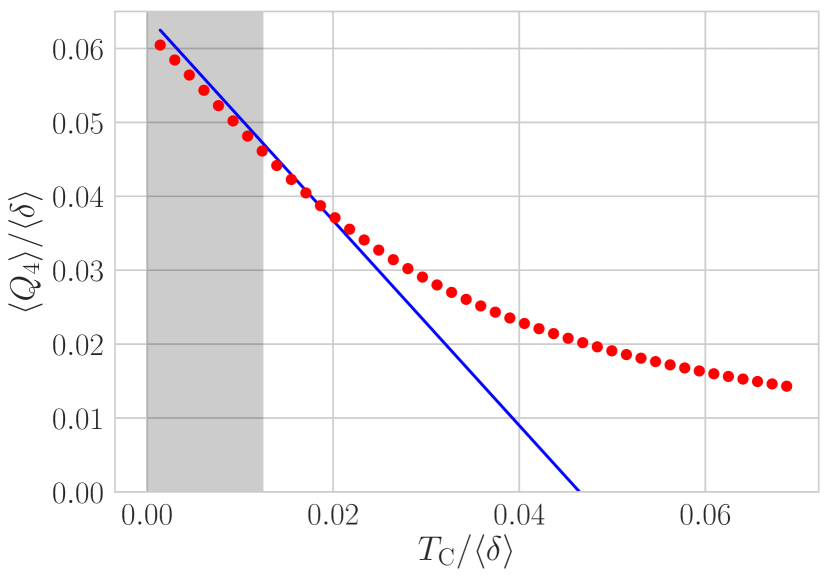
(b) $\left\langle Q_{4}\right\rangle$ vs. $T_{\rm C}$ at $T_{\rm H}=\infty$ and $W_{\rm b}=2^{-4}\left\langle\delta\right\rangle$

(c) $\left\langle Q_{4}\right\rangle$ vs. $\beta_{\rm H}$ at $T_{\rm C}=0$ and $W_{\rm b}=2^{-4}\left\langle\delta\right\rangle$

Figure 8: Average heat $\left\langle Q_{4}\right\rangle$ absorbed during hot thermalization (stroke 4) as a function of (a) the cold-bath bandwidth $W_{\rm b}$, (b) the cold-bath temperature $T_{\rm C}$, and (c) the hot-bath temperature $T_{\rm H}=1/\beta_{\rm H}$: The blue lines represent the analytical prediction (A13), to lowest order in $T_{\rm C}$, with the $\beta_{\rm H}$ dependence of $\left\langle Q_{4}\right\rangle$, too small a correction to include in Eq. (A13): $\left\langle Q_{4}\right\rangle\approx W_{\rm b}-\frac{2\ln 2}{\beta_{\rm C}}+\frac{(W_{\rm b})^{2}}{2\left\langle\delta\right\rangle}\>e^{-N(\beta_{\rm H}\mathcal{E})^{2}/4}$. See Sec. V for other parameters and definitions. The analytics’ shapes agree with the numerics’, and the fit is fairly close, in the appropriate limits (where $e^{-\beta_{\rm C}W_{\rm b}}\ll 1$, $\frac{1}{\beta_{\rm C}\left\langle\delta\right\rangle}\ll 1$, and $\frac{W_{\rm b}}{\left\langle\delta\right\rangle}\ll 1$, in the gray shaded regions). The predictions underestimate $\left\langle Q_{4}\right\rangle$; see the Fig. 7 caption. Figure 8(c) suggests that the numerics deviate significantly from the analytics: The numerics appear to depend on $\beta_{\rm H}$ via a linear term absent from the $\left\langle Q_{4}\right\rangle$ prediction. This seeming mismatch appears symptomatic of finite sample and system sizes.

A 6 Average per-cycle power $\left\langle W_{\rm tot}\right\rangle$

By the first law of thermodynamics, the net work outputted by the engine equals the net heat absorbed. Summing Eqs. (A13) and (A12) yields the per-trial power, or average work outputted per engine cycle:

$$\boxed{\left\langle W_{\rm tot}\right\rangle}=\left\langle Q_{2}\right\rangle+\left\langle Q_{4}\right\rangle\boxed{\approx W_{\rm b}-\frac{2\ln 2}{\beta_{\rm C}}+4\ln 2\>\frac{W_{\rm b}}{\beta_{\rm C}\left\langle\delta\right\rangle}}\,.$$ (A14)

The leading-order $\beta_{\rm H}$ correction is negative and too small to include—of order $\left\langle\delta\right\rangle\left(\frac{W_{\rm b}}{\left\langle\delta\right\rangle}\right)^{2}N\left(\beta_{\rm H}\mathcal{E}\right)^{2}\,.$ Equation (A14) agrees well with the numerics in the appropriate limits ($T_{\rm C}\ll W_{\rm b}\ll\left\langle\delta\right\rangle$) and beyond, as shown in Fig. 9. The main text contains the primary analysis of Eq. (A14). Here, we discuss the $\left\langle Q_{2}\right\rangle$ correction, limiting behaviors, and scaling.

The negative $\left\langle Q_{2}\right\rangle=-\frac{\left(W_{\rm b}\right)^{2}}{\left\langle\delta\right\rangle}$ detracts little from the leading term $W_{\rm b}$ of $\left\langle Q_{4}\right\rangle$: $\frac{(W_{\rm b})^{2}}{\left\langle\delta\right\rangle}\ll W_{\rm b}$, since $\frac{W_{\rm b}}{\left\langle\delta\right\rangle}\ll 1$. The $\left\langle Q_{2}\right\rangle$ cuts down on the per-trial power little.

The limiting behavior of Eq. (A14) makes sense: Consider the limit as $W_{\rm b}\to 0$. The cold bath has too small a bandwidth to thermalize the engine, so the engine should output no work, on averge. Indeed, the first and third terms in Eq. (A14) vanish, being proportional to $W_{\rm b}$. The second term vanishes because $\beta_{\rm C}\to\infty$ more quickly than $W_{\rm b}\to 0\,,$ by Eq. (A2): The cold bath is very cold.

Equation (A14) scales with the system size $N$ no more quickly than $\sqrt{N}/2^{N}$, by the assumption $W_{\rm b}\ll\left\langle\delta\right\rangle\sim\sqrt{N}/2^{N}$. This scaling makes sense: The engine outputs work because the energy eigenvalues meander upward and downward in Fig. 2 as $H(t)$ is tuned. In the thermodynamic limit, levels squeeze together. Energy eigenvalues have little room in which to wander, and the engine outputs little work. Hence our parallelization of fixed-length mesoscopic subengines in the thermodynamic limit (Sec. III).

(a) $\left\langle W_{\rm tot}\right\rangle$ vs. $W_{\rm b}$ at $T_{\rm C}=0$ and $T_{\rm H}=\infty$

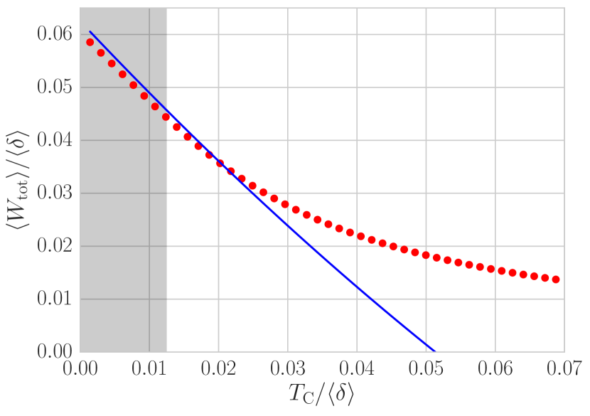
(b) $\left\langle W_{\rm tot}\right\rangle$ vs. $T_{\rm C}$ at $T_{\rm H}=\infty$ and $W_{\rm b}=2^{-4}\left\langle\delta\right\rangle$

(c) $\left\langle W_{\rm tot}\right\rangle$ vs. $\beta_{\rm H}$ at $T_{\rm C}=0$ and $W_{\rm b}=2^{-4}\left\langle\delta\right\rangle$

Figure 9: Per-cycle power $\left\langle W_{\rm tot}\right\rangle$ as a function of (a) the cold-bath bandwidth $W_{\rm b}$, (b) the cold-bath temperature $T_{\rm C}$, and (c) the hot-bath temperature $T_{\rm H}=1/\beta_{\rm H}$: The blue lines represent the analytical prediction $\left\langle W_{\rm tot}\right\rangle\approx W_{\rm b}-\frac{2\ln 2}{\beta_{\rm C}}$: Eq. (A14), to first order in $\frac{W_{\rm b}}{\left\langle\delta\right\rangle}$ and in $\frac{1}{\beta_{\rm C}\left\langle\delta\right\rangle}$. The analytics largely agree with the numerics in the appropriate regime: $\frac{W_{\rm b}}{\left\langle\delta\right\rangle}\ll 1$, and $\frac{T_{\rm C}}{\left\langle\delta\right\rangle}\ll 1$ (in the gray shaded region). Outside that regime, the analytics underestimate $\left\langle W_{\rm tot}\right\rangle$; see Fig. 7 for an analysis. Figure 9(c) suggests that the numerics depend on $\beta_{\rm H}$ via a linear term absent from the analytical prediction; see the caption of Fig. 8(c).

A 7 Efficiency $\eta_{\rm MBL}$ in the adiabatic approximation

The efficiency is defined as

$$\eta_{\rm MBL}:=\frac{\left\langle W_{\rm tot}\right\rangle}{\left\langle Q_{\rm in}\right\rangle}\,.$$ (A15)

The numerator is averaged separately from the denominator because averaging $W_{\rm tot}$ over runs of one mesoscopic engine is roughly equivalent to averaging over simultaneous runs of parallel subengines in one macroscopic engine. $\frac{\left\langle W_{\rm tot}\right\rangle}{\left\langle Q_{\rm in}\right\rangle}$ may therefore be regarded as the $\frac{W_{\rm tot}}{Q_{\rm in}}$ of one macroscopic-engine trial.

The positive-heat-absorbing-stroke is stroke 4, in the average trial:

$$\left\langle Q_{\rm in}\right\rangle=\left\langle Q_{4}\right\rangle=\left\langle W_{\rm tot}\right\rangle-\left\langle Q_{2}\right\rangle=\left\langle W_{\rm tot}\right\rangle\left(1-\frac{\left\langle Q_{2}\right\rangle}{\left\langle W_{\rm tot}\right\rangle}\right)=\left\langle W_{\rm tot}\right\rangle\left(1+\phi\right)\,,$$ (A16)

wherein

$$\phi:=-\frac{\left\langle Q_{2}\right\rangle}{\left\langle W_{\rm tot}\right\rangle}\approx\frac{W_{\rm b}}{2\left\langle\delta\right\rangle}\,.$$ (A17)

Substituting from Eq. (A16) into Eq. (A15) yields

$$\boxed{\eta_{\rm MBL}\approx}\frac{\left\langle W_{\rm tot}\right\rangle}{\left\langle W_{\rm tot}\right\rangle(1+\phi)}\approx 1-\phi=\boxed{1-\frac{W_{\rm b}}{2\left\langle\delta\right\rangle}}\,.$$ (A18)

Using suboptimal baths diminishes the efficiency. Adding $\beta_{\rm C}$-dependent terms from Eq. (A14) to $\left\langle W_{\rm tot}\right\rangle$ yields

$$\phi^{\prime}=\frac{W_{\rm b}}{2\left\langle\delta\right\rangle}+\frac{\ln 2}{\beta_{\rm C}\left\langle\delta\right\rangle}-2\ln 2\>\frac{W_{\rm b}}{\left\langle\delta\right\rangle}\>\frac{1}{\beta_{\rm C}\left\langle\delta\right\rangle}\,.$$ (A19)

The $\beta_{\rm H}$ correction, $1-\frac{W_{\rm b}}{2\left\langle\delta\right\rangle}\>e^{-N(\beta_{\rm H}\mathcal{E})^{2}/4}$, is too small to include. The correction shares the sign of $\beta_{\rm H}$: A lukewarm hot bath lowers the efficiency.

Expressions (A18) and (A19) are compared with results from numerical simulations in Fig. 10. The analytics agree with the numerics in the appropriate regime ($T_{\rm C}\ll W_{\rm b}\ll\left\langle\delta\right\rangle$).

(a) $\eta_{\rm MBL}$ vs. $W_{\rm b}$ at $T_{\rm C}=0$ and $T_{\rm H}=\infty$

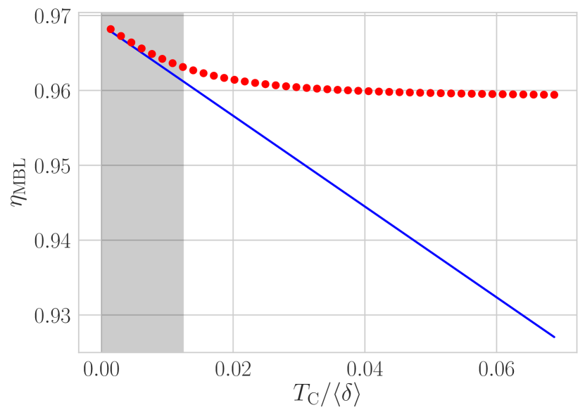
(b) $\eta_{\rm MBL}$ vs. $T_{\rm C}$ at $T_{\rm H}=\infty$ and $W_{\rm b}\approx 10^{-4}\sqrt{N}\mathcal{E}\approx 0.04\left\langle\delta\right\rangle$

(c) $\eta_{\rm MBL}$ vs. $\beta_{\rm H}$ at $T_{\rm C}=0$ and $W_{\rm b}=2^{-4}\left\langle\delta\right\rangle$

Figure 10: Efficiency $\eta_{\rm MBL}$ as a function of (a) the cold-bath bandwidth $W_{\rm b}$, (b) the cold-bath temperature $T_{\rm C}$, and (c) the hot-bath temperature $T_{\rm H}=1/\beta_{\rm H}$: The blue lines represent the analytical predictions (A18) and (A19). Figure (10(c)) shows the leading-order $\beta_{\rm H}$ dependence of $\eta_{\rm MBL}$, a correction too small to include in Eq. (A19): $1-\frac{W_{\rm b}}{2\left\langle\delta\right\rangle}\>e^{-N(\beta_{\rm H}\mathcal{E})^{2}/4}$. See Sec. V for other parameters and definitions. The analytics agree with the numerics fairly well in the appropriate regime ($\frac{W_{\rm b}}{\left\langle\delta\right\rangle}\ll 1$, $\frac{T_{\rm C}}{\left\langle\delta\right\rangle}\ll 1$, and $\sqrt{N}\>T_{\rm H}\mathcal{E}\ll 1$). The analytics underestimate $\eta_{\rm MBL}$; see the Fig. 7 caption.

Appendix B Phenomenological model for the macroscopic MBL Otto engine

The macroscopic MBL Otto engine benefits from properties of MBL (Sec. III), localization and local level repulsion. We understand these properties from Anderson insulators Anderson_58_Absence and perturbation theory. Anderson insulators are reviewed in Sec. B 1. Local level repulsion in Anderson insulators Sivan_87_Energy in the strong-disorder limit is reviewed in Sec. B 2. Section B 3 extends local level repulsion to MBL. Local level repulsion’s application to the MBL engine is discussed in Sec. B 4. Throughout this section, $N$ denotes the whole system’s length.

B 1 Anderson localization

Consider a 1D spin chain or, equivalently, a lattice of spinless fermions. An Anderson-localized Hamiltonian $H_{\rm And}$ has almost the form of Eq. (32), but three elements are removed: the $t$-dependence, $Q\bm{(}h(\alpha_{t})\bm{)}$, and the interaction ($\bm{\sigma}_{j}\cdot\bm{\sigma}_{j+1}$ is replaced with $\sigma_{j}^{+}\,\sigma_{j+1}^{-}+{\rm h.c.}$).

Let $\lvert 0\rangle$ denote some reference state in which all the spins point downward (all the fermionic orbitals are empty). In this section, we focus, for concreteness, on the properties of single-spin excitations relative to $\lvert 0\rangle$ Anderson_58_Absence ; Sivan_87_Energy . The $\ell^{\rm th}$ excitation is represented, in fermionic notation, as $\sum\nolimits_{x}\psi_{\ell}(x)\,\sigma^{+}_{x}|0\rangle$. The single-excitation wave functions $\psi_{\ell}(x)$ are localized: $x_{\ell}$ denotes the point at which the probability density $|\psi_{\ell}(x)|^{2}$ peaks. The wave function decays exponentially with the distance $|x-x_{\ell}|$ from the peak:

$$\psi_{\ell}(x)\approx\sqrt{\frac{2}{\xi_{\rm And}}}\;e^{-|x-x_{\ell}|/\xi_{\rm And}}\,.$$ (B1)

The localization length varies with the Hamiltonian parameters as

$$\xi_{\rm And}\sim\frac{1}{\ln h}$$ (B2)

at large disorder, whose overall strength is $h$.

B 2 Local level repulsion in Anderson insulators

We begin with the infinitely localized limit, $h\rightarrow\infty$. We take $\mathcal{E}\rightarrow 0$ to keep the Hamiltonian’s energy scale finite. The hopping terms can be neglected, and particles on different sites do not repel. Single-particle excitations are localized on single sites. The site-$i$ excitation corresponds to an energy $2\mathcal{E}hh_{i}$. Since the on-site potentials $h\cdot h_{i}$ are uncorrelated, neighboring-site excitations’ energies are uncorrelated.

Let us turn to large but finite $h$. Recall that $h\cdot h_{i}$ is drawn uniformly at random from $[-h,\,h]$. The uniform distribution has a standard deviation of $\frac{h}{\sqrt{3}}\gg 1\,.$ Therefore, $h|h_{i}-h_{i+1}|\gg 1$ for most pairs of neighboring sites. The hopping affects these sites’ wave functions and energies weakly. But with a probability $\sim\frac{1}{h}$, neighboring sites have local fields $h\cdot h_{i}$ and $h\cdot h_{i+1}$ such that $h|h_{i}-h_{i+1}|\lesssim 1$. The hopping hybridizes such sites. The hybridization splits the sites’ eigenvalues by an amount $\sim\sqrt{h^{2}(h_{i}-h_{i+1})^{2}+\mathcal{E}^{2}}\geq\mathcal{E}$.

Consider, more generally, two sites separated by a distance $L\,.$ Suppose that the sites’ disorder-field strengths are separated by $<1/h^{L}$. (The upper bound approximates the probability amplitude associated with a particle’s hopping the $L$ intervening sites). The sites’ excitation energies and energy eigenfunctions are estimated perturbatively. The expansion parameter is $1/h\,.$ To zeroth order, the energies are uncorrelated and (because $h|h_{i}-h_{i+L}|<1/h^{L}$) are split by $<\mathcal{E}/h^{L}\,.$ The eigenfunctions are hybridized at order $L\,.$ The perturbed energies are split by $\geq\mathcal{E}/h^{L}\sim\mathcal{E}e^{-L/\xi_{\rm And}}\,.$ [Recall that $\xi_{\rm And}\sim 1/\ln h$, by Eq. (B2).]

Hence eigenstates localized on nearby sites have correlated energies: The closer together sites lie in real space, the lower the probability that they correspond to similar energies. This conclusion agrees with global Poisson statistics: Consider a large system of $N\gg 1$ sites. Two randomly chosen single-particle excitations are typically localized a distance $\sim N$ apart. The argument above implies only that the energies lie $>\mathcal{E}e^{-N/\xi_{\rm And}}$ apart. This scale is exponentially smaller (in $N$) than the average level spacing $\sim\frac{\mathcal{E}h}{N}$ between single-particle excitations.

We can quantify more formally the influence of hybridization on two energies separated by $\omega$ and associated with eigenfunctions localized a distance $L$ apart. The level correlation function is defined as

$$R(L,\omega):=\frac{1}{N^{2}}\sum_{i,n,n^{\prime}}|\langle 0|\sigma^{-}_{i}|n\rangle|^{2}\,|\langle 0|\sigma^{-}_{i+L}|n^{\prime}\rangle|^{2}\,\delta(E_{n}-E_{n^{\prime}}-\omega)-\tilde{\mu}(\omega)^{2}\,.$$ (B3)

The spatially averaged density of states at frequency $\omega$ is denoted by $\tilde{\mu}(\omega):=\frac{1}{N}\sum_{n}|\langle 0|\sigma^{-}_{i}|n\rangle|^{2}\,\delta(E_{n}-\omega)$. $|n\rangle$ and $|n^{\prime}\rangle$ denote eigenstates, corresponding to single-particle excitations relative to $|0\rangle$, associated with energies $E_{n}$ and $E_{n^{\prime}}$. In the Anderson insulator, $R(L,\omega)\approx 0$ when $\omega\gg\mathcal{E}e^{-L/\xi_{\rm And}}$: Levels are uncorrelated when far apart in space and/or energy. When energies are close ($\omega\lesssim\mathcal{E}e^{-L/\xi_{\rm And}}$), $R(L,\omega)$ is negative. These levels repel (in energy space).

B 3 Generalization to many-body localization

The estimates above can be extended from single-particle Anderson-localized systems to MBL systems initialized in arbitrary energy eigenstates (or in position-basis product states). $R(L,\omega)$ is formulated in terms of matrix elements $\langle 0|\sigma_{i}^{-}|n\rangle$ of local operators $\sigma_{i}^{-}$. The local operators relevant to Anderson insulators have the forms of the local operators relevant to MBL systems. Hence $R(L,\omega)$ is defined for MBL as for Anderson insulators. However, $\lvert 0\rangle$ now denotes a generic many-body state.

Let us estimate the scale $\mathcal{J}_{L}$ of the level repulsion between MBL energies, focusing on exponential behaviors. The MBL energy eigenstates result from perturbative expansions about Anderson energy eigenstates. Consider representing the Hamiltonian as a matrix $\mathcal{M}$ with respect to the true MBL energy eigenbasis. Off-diagonal matrix elements couple together unperturbed states. These couplings hybridize the unperturbed states, forming corrections. The couplings may be envisioned as rearranging particles throughout a distance $L$.

MBL dynamics is unlikely to rearrange particles across considerable distances, due to localization. Such a rearrangement is encoded in an off-diagonal element $\mathcal{M}_{ij}$ of $\mathcal{M}$. This $\mathcal{M}_{ij}$ must be small—suppressed exponentially in $L$. $\mathcal{M}_{ij}$ also forces the eigenstates’ energies apart, contributing to level repulsion (NYH_17_MBL, , App. F). Hence the level-repulsion scale is suppressed exponentially in $L$:

$$\mathcal{J}_{L}\sim\mathcal{E}e^{-L/\zeta}\,,$$ (B4)

for some $\zeta\,.$ At infinite temperature, $\zeta$ must $<\frac{1}{\ln 2}$ for the MBL phase to remain stable mbmott . Substituting into Eq. (B4) yields $\mathcal{J}_{L}<\frac{\mathcal{E}}{2^{L}}$. The level-repulsion scale is smaller than the average gap.

The size and significance of $\mathcal{J}_{L}$ depend on the size of $L$. At the crossover distance $\xi$, the repulsion $\mathcal{J}_{L}$ (between energy eigenfunctions localized a distance $\xi$ apart) becomes comparable to the average gap $\sim\frac{\mathcal{E}}{2^{\xi}}$ between the eigenfunctions in the same length-${\xi}$ interval: $\mathcal{E}e^{-{\xi}/\zeta}\sim\frac{1}{e}\,\frac{\mathcal{E}}{2^{\xi}}\,.$ Solving for the crossover distance yields

$$\xi\sim\frac{1}{\frac{1}{\zeta}-\ln 2}\,.$$ (B5)

Relation (B5) provides a definition of the MBL localization length $\xi\,.$ [This $\xi$ differs from the Anderson localization length $\xi_{\rm And}$, Eq. (B2).] Solving for $\zeta$ yields

$$\zeta\sim\frac{1}{\frac{1}{\xi}+\ln 2}\,.$$ (B6)

The MBL Otto cycle involves two localization lengths in the thermodynamic limit. In the shallowly localized regime, $\xi=\xi_{>}\,.$ Each eigenfunction has significant weight on $\xi_{>}\approx 10$ sites, in an illustrative example. In the highly localized regime, $\xi=\xi_{<}\,.$ Eigenfunctions peak tightly: $\xi_{<}\approx 1\,.$

Suppose that the particles are rearranged across a large distance $L\gg\xi$. The level-repulsion scale

$$\boxed{\mathcal{J}_{L\gg\xi}\sim\mathcal{E}e^{-L/\xi}\;2^{-L}}\,.$$ (B7)

In the MBL engine’s very localized regime, in which $\xi=\xi_{<}$, if $L=\xi_{>}$ equals one subengine’s length, $\mathcal{J}_{L\gg\xi}=\delta_{-}$.

Now, suppose that particles are rearranged across a short distance $L\lesssim\xi$. Random-matrix theory approximates this scenario reasonably (while slightly overestimating the level repulsion). We can approximate the repulsion between nearby-eigenfunction energies with the average gap $\left\langle\delta\right\rangle^{(L)}$ in the energy spectrum of a length-$L$ system:

$$\boxed{\mathcal{J}_{L\leq\xi}\sim\left\langle\delta\right\rangle^{(L)}\sim\frac{\mathcal{E}}{2^{L}}}\,.$$ (B8)

B 4 Application of local level repulsion to the MBL Otto engine in the thermodynamic limit

Consider perturbing an MBL system locally. In the Heisenberg picture, the perturbing operator spreads across a distance $L(t)\sim\zeta\ln(\mathcal{E}t)$ Nandkishore_15_MBL . (See also Khemani_15_NPhys_Nonlocal .) The longer the time $t$ for which the perturbation lasts, the farther the influence spreads.

Consider tuning the Hamiltonian infinitely slowly, to preclude diabatic transitions: $t\to\infty\,.$ Even if the Hamiltonian consists of spatially local terms, the perturbation to each term spreads across the lattice. The global system cannot be subdivided into independent subengines. The global system’s average gap vanishes in the thermodynamic limit: $\left\langle\delta\right\rangle\to 0\,.$ Since $\left\langle W_{\rm tot}\right\rangle\sim W_{\rm b}\ll\left\langle\delta\right\rangle$, the per-cycle power seems to vanish in the thermodynamic limit: $W_{\rm b}\to 0$.

Now, consider tuning the Hamiltonian at a finite speed $v$. Dimensional analysis suggests that the relevant time scale is $t\sim\frac{\mathcal{E}}{v}\,.$ Local perturbations affect a region of length $\sim L(\mathcal{E}/v)\sim\zeta\ln(\mathcal{E}^{2}/v)$. On a length scale $L(\mathcal{E}/v)$, global level correlations govern the engine’s performance less than local level correlations do, i.e., less than $R\bm{(}L(\mathcal{E}/v),\omega\bm{)}$ does. This correlator registers level repulsion at a scale independent of $N$. Finite-speed tuning renders finite the average gap accessible to independent subengines, the $\left\langle\delta\right\rangle$ that would otherwise close in the thermodynamic limit. Each mesoscale subengine therefore outputs $\left\langle W_{\rm tot}\right\rangle>0\,.$

We can explain the gap’s finiteness differently: Suppose that the engine’s state starts some trial with weight on the $j^{\rm th}$ energy level. The eigenenergies wiggle up and down during stroke 1. The $j^{\rm th}$ energy may approach the $(j-1)^{\rm th}$. Such close-together energies likely correspond to far-apart subengines. If the levels narrowly avoided crossing, particles would be rearranged across a large distance. Particles must not be, as subengines must function independently. Hence the engine must undergo a diabatic transition: The engine’s state must retain its configuration. The engine must behave as though the approaching energy level did not exist. Effectively removing the approaching level from the available spectrum effectively creates a gap in the spectrum. One can create such an effective gap (can promote such diabatic transitions) by tuning the Hamiltonian at a finite $v$.

Appendix C Constraint 2 on cold thermalization: Suppression of high-order-in-the-coupling energy exchanges

Section IV introduces the dominant mechanism by which the bath changes a subengine’s energy. The energy changes by an amount $\sim W_{\rm b}$, at a rate $\sim g$. Higher-order processes can change the subengine energy by amounts $>W_{\rm b}$ and operate at rates $O(g^{\ell})$, wherein $\ell\geq 2$. The subengine should thermalize across just small gaps $\delta\leq W_{\rm b}$. Hence the rate-$g^{\ell}$ processes must operate much more slowly than the rate-$g$ processes: $g$ must be small. We describe the higher-order processes, upper-bound $g$, and lower-bound $\tau_{\rm th}$.

The higher-order processes can be understood as follows. Let $H_{\rm tot}=H_{\rm macro}(t)+H_{\rm bath}+H_{\rm int}$ denote the Hamiltonian that governs the engine-and-bath composite. $H_{\rm tot}$ generates the time-evolution operator $U(t):=e^{-iH_{\rm tot}t}$. Consider Taylor-expanding $U(t)$. The $\ell^{\rm th}$ term is suppressed in $g^{\ell}$, contains $2\ell$ fermion operators $c_{j}$ and $c_{j^{\prime}}^{\dagger}$, and contains $\ell$ boson operators $b_{\omega}$ and $b_{\omega^{\prime}}^{\dagger}$. This term encodes the absorption, by the bath, of $\ell$ energy quanta of sizes $\leq W_{\rm b}$. The subengine gives the bath a total amount $\sim\ell W_{\rm b}$ of heat. The subengine should not lose so much heat. Hence higher-order processes should occur much more slowly than the rate-$g$ processes:

$$\tau_{\rm high-ord.}\gg\tau_{\rm th}\,.$$ (C1)

Let us construct an expression for the left-hand side. Which processes most urgently require suppressing? Processes that change the subengine’s energy by $\gtrsim\left\langle\delta\right\rangle$. Figure 2 illustrates why. If the right-hand leg has length $\gtrsim\left\langle\delta\right\rangle$, the right-hand leg could be longer than the left-hand leg. If it were, the trial would yield net negative work, $W_{\rm tot}<0$. The bath would absorb energy $\left\langle\delta\right\rangle$ from a subengine by absorbing $\sim\frac{\left\langle\delta\right\rangle}{W_{\rm b}}$ packets of energy $\sim W_{\rm b}$ each. Hence the bath would appear to need to flip $\sim L=\frac{\left\langle\delta\right\rangle}{W_{\rm b}}$ spins to absorb energy $\sim\left\langle\delta\right\rangle$. (We switch from fermion language to spin language for convenience.) However, the length-$L$ spin subchain has a discrete effective energy spectrum. The spectrum might lack a level associated with the amount $\text{(initial energy)}-\left\langle\delta\right\rangle$ of energy. If so, the bath must flip more than $\frac{\left\langle\delta\right\rangle}{W_{\rm b}}$ spins—local level correlations suggest $\sim\xi_{>}$ spins (App. B). Hence $L=\max\left\{\frac{\left\langle\delta\right\rangle}{W_{\rm b}},\xi_{>}\right\}$. Energy is rearranged across the distance $L$ at a rate $\propto g^{L}$.

Having described the undesirable system-bath interactions, we will bound $g$ via Fermi’s Golden Rule, Eq. (29). Let $\Gamma_{fi}\sim 1/\tau_{\rm high-ord.}$ now denote the rate at which order-$g^{L}$ interactions occur. The bath DOS remains $\mu_{\rm bath}(E_{if})\sim\frac{1}{W_{\rm b}}$. Let us estimate the matrix-element size $|\langle f|V|i\rangle|$. The bath flips each spin at a rate $g$ (modulo a contribution from the bath’s DOS). Flipping one spin costs an amount $\sim\mathcal{E}$ of energy, on average. [$\mathcal{E}$ denotes the per-site energy density, as illustrated in Eq. (32).] Hence $L$ spins are flipped at a rate $\sim\mathcal{E}\left(\frac{g}{\mathcal{E}}\right)^{L}$. The initial $\mathcal{E}$ is included for dimensionality. We substitute into Fermi’s Golden Rule [Eq. (29)], then solve for the time:

$$\tau_{\rm high-ord.}\sim\frac{W_{\rm b}\,\mathcal{E}^{2\left(L-1\right)}}{g^{2L}}\,\quad\text{wherein}\quad L=\max\left\{\frac{\left\langle\delta\right\rangle}{W_{\rm b}},\>\xi_{>}\right\}\,.$$ (C2)

We substitute from Eqs. (C2) and (30) into Ineq. (C1). Solving for the coupling yields

$$g\ll\mathcal{E}\cdot\left(\frac{\delta_{-}}{\mathcal{E}}\right)^{1/(L-1)}\,\quad\text{wherein}\quad L=\max\left\{\frac{\left\langle\delta\right\rangle}{W_{\rm b}},\>\xi_{>}\right\}\,.$$ (C3)

Substituting back into Eq. (30) yields a second bound on $\tau_{\rm th}$:

$$\boxed{\tau_{\rm th}\gg\frac{W_{\rm b}}{\delta_{-}^{2}}\left(\frac{\mathcal{E}}{\delta_{-}}\right)^{1/(L-1)}\,,\quad\text{wherein}\quad L=\max\left\{\frac{\left\langle\delta\right\rangle}{W_{\rm b}},\>\xi_{>}\right\}}\,.$$ (C4)

Let us express the bound in terms of localization lengths. We set $W_{\rm b}\sim\frac{\left\langle\delta\right\rangle}{10}$ and approximate $L\pm 1\sim L\sim\xi_{>}$. We substitute in for $\left\langle\delta\right\rangle$ from Eq. (B8) and for $\delta_{-}$ from Eq. (B7):

$$\boxed{\tau_{\rm th}\gg\frac{1}{10\mathcal{E}}\>e^{2\xi_{>}/\xi_{<}}\>2^{2\xi_{>}}}\,.$$ (C5)

This inequality is looser than Ineq. (31): The no-higher-order-processes condition is less demanding than Markovianity.

Appendix D Numerical simulations of the MBL Otto engine

We simulated one 12-site mesoscale engine at half-filling. (We also studied other system sizes, to gauge finite-size effects.) Our code is available at https://github.com/christopherdavidwhite/MBL-mobile. The random-field Heisenberg Hamiltonian (32) governed the system. We will drop the subscript from $H_{\rm sim}(t)$.

Call the times at which the strokes end $t=\tau,\tau^{\prime},\tau^{\prime\prime},$ and $\tau^{\prime\prime\prime}$ (see Fig. 3). For each of $N_{\rm reals}\approx 1,000$ disorder realizations, we computed the whole density matrix $\rho(t)$ at $t=0,\tau,\tau^{\prime},\tau^{\prime\prime},\tau^{\prime\prime\prime}$. (See App. D 3 i and D 4 for an explanation of how.) The engine’s time-$t$ internal energy is $E(t)={\rm Tr}\bm{(}H(t)\rho(t)\bm{)}\,.$ The quantities of interest are straightforwardly

$$\langle W_{1}\rangle=E(0)-E(\tau)\,,\quad\langle W_{3}\rangle=E(\tau^{\prime\prime\prime})-E(\tau^{\prime\prime})\,,$$ (D1)

$$\langle Q_{2}\rangle=E(\tau^{\prime\prime})-E(\tau^{\prime})\,,\quad\text{and}\quad\langle Q_{4}\rangle=E(0)-E(\tau^{\prime\prime\prime})\,.$$ (D2)

We disorder-averaged these quantities before dividing to compute the efficiency, $\eta_{\rm MBL}=1-\frac{\left\langle W_{1}\right\rangle+\left\langle W_{3}\right\rangle}{\left\langle Q_{4}\right\rangle}\,.$

D 1 Scaling factor

We wish to keep the DOS constant through the cycle. To fix $\mu(E)$, we rescale the Hamiltonian by a factor $Q\bm{(}h(\alpha_{t})\bm{)}$. We define $Q^{2}\bm{(}h(\alpha_{t})\bm{)}$ as the disorder average of the variance of the unrescaled DOS:

$$Q^{2}\bm{(}h(\alpha_{t})\bm{)} :=\Bigg{\langle}\Bigg{(}\frac{1}{\mathcal{N}}\sum_{j=1}^{\mathcal{N}}E_{j}^{2}\Bigg{)}-\Bigg{(}\frac{1}{\mathcal{N}}\sum_{j=1}^{\mathcal{N}}E_{j}\Bigg{)}^{2}\Bigg{\rangle}_{\rm disorder}=\Bigg{\langle}\frac{1}{\mathcal{N}}{\rm Tr}\bm{(}\tilde{H}^{2}(t)\bm{)}-\Bigg{(}\frac{1}{\mathcal{N}}{\rm Tr}\bm{(}\tilde{H}(t)\bm{)}\Bigg{)}^{2}\Bigg{\rangle}_{\rm disorder}\,.$$ (D3)

The $\tilde{H}(t)$ denotes an unrescaled variation on the random-field Heisenberg Hamiltonian $H(t)$ of Eq. (32):

$$\tilde{H}(t):=\mathcal{E}\left[\sum_{j=1}^{N-1}\bm{\sigma}_{j}\cdot\bm{\sigma}_{j+1}+h(\alpha_{t})\sum_{j=1}^{N}h_{j}\sigma_{j}^{z}\right]\,.$$ (D4)

To compute $Q^{2}\bm{(}h(\alpha_{t})\bm{)}$, we rewrite the unrescaled Hamiltonian as

$$\tilde{H}(t)=\mathcal{E}\left[2\sum_{j=1}^{N-1}\left(\sigma^{+}_{j}\sigma^{-}_{j+1}+{\rm h.c.}\right)+\sum_{j=1}^{N-1}\sigma^{z}_{j}\sigma^{z}_{j+1}+h(\alpha_{t})\sum_{j=1}^{N}h_{j}\sigma^{z}_{j}\right]\,.$$ (D5)

We assume that $N$ is even, and we work at half-filling. The $\frac{N}{2}$-particle subspace has dimensionality $\mathcal{N}={N\choose N/2}\,.$

Let us calculate some operator traces that we will invoke later. Let $X:=\prod_{j=1}^{N}\sigma^{x}$ denote the global spin-flip operator. For any operator $A$ such that $X^{\dagger}AX=-A$,

$${\rm Tr}(A)={\rm Tr}\left(X^{\dagger}AX\right)=-{\rm Tr}(A)\,.$$ (D6)

We have used the evenness of $N$, which implies the invariance of the half-filling subspace under $X$. Also, ${\rm Tr}(A)=0$. In particular, $0={\rm Tr}(\sigma^{z}_{j})={\rm Tr}(\sigma^{z}_{j}\sigma^{z}_{j^{\prime}}\sigma^{z}_{j^{\prime\prime}})$, if $j\neq j^{\prime}\neq j^{\prime\prime}$.

Traces of products of even numbers of $\sigma^{z}$ factors require more thought:

$${\rm Tr}(\sigma^{z}_{j}\sigma^{z}_{j+1}) =(\text{\# states $j,j+1=\uparrow\uparrow$})+(\text{\# states $j,j+1=\downarrow\downarrow$})-2(\text{\# states $j,j+1=\uparrow\downarrow$})$$

$$={{N-2}\choose{N/2-2}}+{{N-2}\choose{N/2}}-2{{N-2}\choose{N/2-1}}$$

$$=-\mathcal{N}\frac{1}{N-1}\,.$$ (D7)

Similarly,

$${\rm Tr}\left([\sigma^{+}_{j}\sigma^{-}_{j}][\sigma^{-}_{j+1}\sigma^{+}_{j+1}]\right) ={\rm Tr}\left([\sigma^{-}_{j}\sigma^{+}_{j}][\sigma^{+}_{j+1}\sigma^{-}_{j+1}]\right)=(\text{\# states $j,j+1=\uparrow\downarrow$})={{N-2}\choose{N/2-1}}$$ (D8)

$$=\mathcal{N}\frac{N}{4(L-1)}\,,$$ (D9)

and

$${\rm Tr}\left(\sigma^{z}_{j}\sigma^{z}_{j+1}\sigma^{z}_{j^{\prime}}\sigma^{z}_{j^{\prime}+1}\right) =(\text{\# states $j,j+1,j^{\prime},j^{\prime}+1=\uparrow\uparrow\uparrow\uparrow$})+{4\choose 2}(\text{\# states $j,j+1,j^{\prime},j^{\prime}+1=\uparrow\uparrow\downarrow\downarrow$})$$

$$\quad+(\text{\# states $j,j+1,j^{\prime},j^{\prime}+1=\downarrow\downarrow\downarrow\downarrow$})$$

$$\quad-{4\choose 1}(\text{\# states $j,j+1,j^{\prime},j^{\prime}+1=\uparrow\uparrow\uparrow\downarrow$})-{4\choose 1}(\text{\# states $j,j+1,j^{\prime},j^{\prime}+1=\uparrow\downarrow\downarrow\downarrow$})$$

$$={{N-4}\choose{N/2-4}}+6{{N-4}\choose{N/2-2}}+{{N-4}\choose{N/2}}-6{{N-4}\choose{N/2-3}}-6{{N-4}\choose{N/2-1}}$$

$$=\mathcal{N}\frac{3}{(N-1)(N-3)}\,,$$ (D10)

wherein the first equality’s combinatorial factors come from permutations on sites $j$, $j+1$, $j^{\prime}$, and $j^{\prime}+1$.

Assembling these pieces, we find ${\rm Tr}\bm{(}\tilde{H}(t)\bm{)}=\mathcal{E}\sum_{j=1}^{N-1}{\rm Tr}\left(\sigma^{z}_{j}\sigma^{z}_{j}\right)=-\mathcal{E}\mathcal{N}.$ Next, we compute ${\rm Tr}\bm{(}\tilde{H}^{2}(t)\bm{)}$:

$$\tilde{H}^{2}(t) =\mathcal{E}^{2}\Bigg{[}4\sum_{j}^{N-1}(\sigma^{+}_{j}\sigma^{-}_{j})(\sigma^{-}_{j+1}\sigma^{+}_{j+1})+4\sum_{j}^{N-1}(\sigma^{-}_{j}\sigma^{+}_{j})(\sigma^{+}_{j+1}\sigma^{-}_{j+1})+\sum_{j,j^{\prime}=1}^{N-1}\sigma^{z}_{j}\sigma^{z}_{j+1}\sigma^{z}_{j^{\prime}}\sigma^{z}_{j^{\prime}+1}+h^{2}(\alpha_{t})\sum_{j=1}^{N}h_{j}^{2}$$

$$\qquad\quad+(\text{traceless terms})\Bigg{]}$$ (D11)

$$=\mathcal{E}^{2}\Bigg{[}4\sum_{j}^{N-1}(\sigma^{+}_{j}\sigma^{-}_{j})(\sigma^{-}_{j+1}\sigma^{+}_{j+1})+4\sum_{j}^{N-1}(\sigma^{-}_{j}\sigma^{+}_{j})(\sigma^{+}_{j+1}\sigma^{-}_{j+1})+\sum_{j=1}^{N-1}\mathbbm{1}+\sum_{j=1}^{N-2}\sigma^{z}_{j}\sigma^{z}_{j+2}$$

$$\qquad\quad+\sum_{j=1}^{N-3}\sum_{j^{\prime}=j+2}^{N-1}\sigma^{z}_{j}\sigma^{z}_{j+1}\sigma^{z}_{j^{\prime}}\sigma^{z}_{j^{\prime}+1}+h(\alpha_{t})^{2}(\alpha_{t})\sum_{j=1}^{N}h_{j}^{2}+(\text{traceless terms})\Bigg{]}\,.$$ (D12)

We take the trace, using Eqs. (D 1), (D8), and (D 1):

$${\rm Tr}\bm{(}\tilde{H}^{2}(t)\bm{)}=\mathcal{N}\Bigg{[}3N-1+\frac{N-2}{N-1}+h^{2}\sum_{j=1}^{N}h_{j}^{2}\Bigg{]}\,.$$ (D13)

We disorder-average by taking $h_{j}^{2}\mapsto\int_{0}^{1}dh_{j}h_{j}^{2}=\frac{1}{3}$:

$$\Big{\langle}{\rm Tr}(H^{2}(t))\Big{\rangle}_{\text{disorder}}=\mathcal{N}\Bigg{[}3N-1+\frac{N-2}{N-1}+N\frac{h^{2}}{3}\Bigg{]}\,.$$ (D14)

Substituting into Eq. (D3), we infer the rescaling factor’s square:

$$Q^{2}\bm{(}h(\alpha_{t})\bm{)}=3N-2+\frac{N-2}{N-1}+N\frac{h^{2}}{3}\,.$$ (D15)

Our results are insensitive to the details of $Q$. The width of the DOS in one disorder realization will differ from the disorder average (D15). Moreover, that difference will vary as we tune $h(\alpha_{t})$, because the disorder affects only one term. The agreement between the analytics, in which $\mu(E)$ is assumed to remain constant in $t$, and the numerics is therefore comforting: The engine is robust against small variations in the rescaling.

D 2 Representing states and Hamiltonians

We structured our software to facilitate a possible extension: The cold bath might be modeled more realistically, as coupling to the engine only locally.

We represent the state of one mesoscopic MBL Otto engine with a density matrix $\rho\in\mathbb{C}^{\mathcal{N}\times\mathcal{N}}\,,$ and the Hamiltonian with a matrix $H\in\mathbb{C}^{\mathcal{N}\times\mathcal{N}}\,,$ relative to the basis $\left\{\lvert s_{1}\rangle,\ldots,\lvert s_{\mathcal{N}}\rangle\right\}=\left\{\lvert\uparrow\ldots\uparrow\rangle,\ldots,\lvert\downarrow\ldots\downarrow\rangle\right\}$ of products of $\sigma^{z}$ eigenstates. We track the whole density matrix, rather than just the energy-diagonal elements, with an eye toward the coherent superpositions that diabatic corrections create. For an $N$-site chain at half-filling, $\mathcal{N}={N\choose N/2}\simeq\sqrt{\frac{2}{\pi N}}\>2^{N}\,.$

D 3 Strokes 1 and 3: Tuning

Simulating diabatic evolution requires a different strategy from simulating adiabatic evolution. We describe the latter in Sec. D 3 i and the former in Sec. D 3 ii.

D 3 i Adiabatic evolution

The $(l,m)$ entry of the initial-state density matrix is

$$\rho(0)_{lm}=\langle s_{l}\rvert\frac{1}{Z}e^{-\beta_{\rm H}H(0)}\lvert s_{m}\rangle=\frac{1}{Z}\sum_{j}e^{-\beta_{\rm H}E_{j}(0)}\langle s_{l}\lvert E_{j}(0)\rangle\langle E_{j}(0)\lvert s_{m}\rangle\,.$$ (D16)

The $j^{\rm th}$ eigenstate of $H(0)$, associated with energy $E_{j}(0)$, is denoted by $\lvert E_{j}(0)\rangle$. We approximate the time evolution from $0$ to $\tau$ (during stroke 1) as adiabatic. The evolution therefore does not move weight between levels:

$$\rho(\tau)_{lm}=\frac{1}{Z}\sum_{j}e^{-\beta_{\rm H}E_{j}(0)}\langle s_{l}\lvert E_{j}(\tau)\rangle\langle E_{j}(\tau)\lvert s_{m}\rangle\,.$$ (D17)

If we represented our density matrix relative to an instantaneous energy eigenbasis, simulating the time evolution would be trivial: We would reinterpret the diagonal matrix $\rho$ as being diagonal, with the same elements in a new basis. However, we wish to represent $\rho(t)$ relative to the $\sigma_{j}^{z}$ product basis. This representation enhances the code’s flexibility, facilitating the inclusion of diabatic evolutions and a more detailed model of cold thermalization. To represent $\rho(t)$ relative to the $\sigma_{j}^{z}$ product basis, we note that

$$\rho(\tau)_{lm}=\sum_{j}\langle s_{l}\lvert E_{j}(\tau)\rangle\langle E_{j}(0)\rvert\rho(0)\lvert E_{j}(0)\rangle\langle E_{j}(\tau)\lvert s_{m}\rangle=[U(\tau,0)\rho(0)U(\tau,0)^{\dagger}]_{lm}\,.$$ (D18)

We have defined a time-evolution matrix $U(\tau,0)\in\mathbf{C}^{\mathcal{N}\times\mathcal{N}}$ by $U(\tau,0)_{lm}=\sum_{j}\langle s_{l}\lvert E_{j}(\tau)\rangle\langle E_{j}(0)\lvert s_{m}\rangle\,.$ This matrix is easily computed via exact diagonalization of $H(0)$ and $H(\tau)$.

We can compute the density matrix $\rho(\tau^{\prime\prime})$ at the end of stroke 3 (the tuning from MBL to GOE) from the density matrix $\rho(\tau^{\prime})$ at the end of stroke 2 (the cold-bath thermalization) similarly: $\rho(\tau^{\prime\prime})=U(\tau^{\prime\prime},\tau^{\prime})\rho(\tau^{\prime})U(\tau^{\prime\prime},\tau^{\prime})^{\dagger}\,.$ The time-evolution matrix $U(\tau^{\prime\prime},\tau^{\prime})\in\mathbf{C}^{\mathcal{N}\times\mathcal{N}}$ is given by $U(\tau^{\prime\prime},\tau^{\prime})_{lm}=\sum_{j}\langle s_{l}\lvert E_{j}(0)\rangle\langle E_{j}(\tau)\lvert s_{m}\rangle\,.$ [Recall that $H(\tau^{\prime\prime})=H(0)$ and $H(\tau^{\prime})=H(\tau)$.]

D 3 ii Diabatic (finite-time) evolution

We simulate a stepwise tuning, taking

$$\alpha(t)=\frac{\delta t\,\lfloor t/\delta t\rfloor}{T}\,,$$ (D19)

wherein $\delta t$ denotes a time-step size and $T\propto(h_{\rm MBL}-h_{\mathrm{GOE}})/v$ denotes the total tuning time. To do this, we compute a time-evolution unitary for the whole stroke by chaining together the unitaries for each time step. For stroke 1,

$$U(\tau,0;v,\delta t)=e^{-iH(\tau-\delta t)\delta t}e^{-iH(\tau-2\delta t)\delta t}\dots e^{-iH(0)\delta t}\,,$$ (D20)

with the number of time steps set by the speed. We use the time step $\delta t=0.405\left\langle\delta\right\rangle$, but our results are not sensitive to the time step’s size.

In judging the engine’s effectiveness at a finite $v$, we must estimate the level-repulsion scale $\delta_{-}$. We do this by diagonalizing $10^{6}$ disorder realizations at the relevant disorder width, $h=20$, for $N=8$ sites. A histogram of the gaps is plotted in Fig. 11. We then visually estimate the point at which the distribution turns over. Our results are not sensitive to this value.

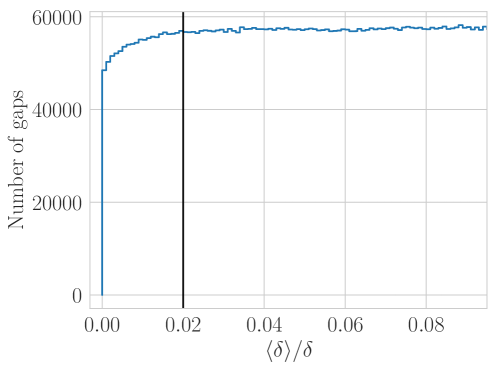
Figure 11: Level-spacing distribution for $10^{6}$ disorder realizations of the random-field Heisenberg model at disorder width $h=20$ and system size $N=8$ (blue line). The vertical black line shows the estimate of the level-repulsion parameter $\delta_{-}$.

D 4 Stroke 2: Thermalization with the cold bath

During stroke 2, the system thermalizes with a bandwidth-$W_{\rm b}$ cold bath. We make three assumptions. First, the bandwidth cutoff is hard: The bath can transfer only amounts $<W_{\rm b}$ of energy at a time. Therefore, the cold bath cannot move probability mass between adjacent levels separated by just one gap $\delta^{\prime}>W_{\rm b}$. Second, the bath is Markovian. Third, the system thermalizes for a long time. The bath has time to move weight across sequences of small gaps $\delta^{\prime}_{j},\delta^{\prime}_{j+1},\ldots<W_{\rm b}$.

We can implement thermalization as follows. First, we identify sequences of levels connected by small gaps. Second, we reapportion weight amongst the levels according to a Gibbs distribution.

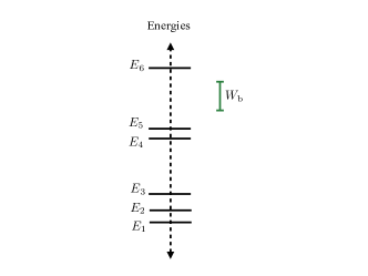
Figure 12: Energies of a cold-thermalized many-body-localized system: We illustrate our implementation of cold thermalization with this example chain of six energies. The cold bath has a bandwidth of size $W_{\rm b}$, depicted in green.

Suppose, for example, that the MBL Hamiltonian $H(\tau)$ contains the following chain of six energies, $E_{1},\dots,E_{6}$, separated from its surrounding levels by large gaps (Fig. 12):

$$(E_{2}-E_{1}),(E_{3}-E_{2})<W_{\rm b}\,,\quad(E_{5}-E_{4})<W_{\rm b}\,,\quad\text{and}\quad(E_{4}-E_{3}),(E_{6}-E_{5})>W_{\rm b}\,.$$ (D21)

We suppress the time arguments to simplify notation. Before thermalization, the density operator is diagonal with respect to the energy basis: $\rho(\tau)=\sum_{j}\rho_{j}\lvert E_{j}\rangle\!\langle E_{j}\rvert\,.$ The weight on level $j$ is denoted by $\rho_{j}$. Thermalization maps

$$\rho(\tau)\mapsto\rho(\tau^{\prime}) =\frac{\rho_{1}+\rho_{2}+\rho_{3}}{e^{-\beta_{\rm C}E_{1}}+e^{-\beta_{\rm C}E_{2}}+e^{-\beta_{\rm C}E_{3}}}\Big{(}e^{-\beta_{\rm C}E_{1}}\lvert E_{1}\rangle\!\langle E_{1}\rvert+e^{-\beta_{\rm C}E_{2}}\lvert E_{2}\rangle\!\langle E_{2}\rvert+e^{-\beta_{\rm C}E_{3}}\lvert E_{3}\rangle\!\langle E_{3}\rvert\Big{)}$$

$$\quad+\frac{\rho_{4}+\rho_{5}}{e^{-\beta_{\rm C}E_{4}}+e^{-\beta_{\rm C}E_{5}}}\Big{(}e^{-\beta_{\rm C}E_{4}}\lvert E_{4}\rangle\!\langle E_{4}\rvert+e^{-\beta_{\rm C}E_{5}}\lvert E_{5}\rangle\!\langle E_{5}\rvert\Big{)}+\rho_{6}\lvert E_{6}\rangle\!\langle E_{6}\rvert\,.$$ (D22)

Appendix E Comparisons with competitor Otto engines

This appendix contains further analysis of the bandwidth engine (Sec. E 1) and introduces an MBL engine tuned between equal-strength disorder realizations (Sec. E 2). Section E 2 compares with an MBL engine thermalized with an ordinary-bandwidth cold bath. The quantum-dot and Anderson-localized engines are elaborated on in Apps. E 3 and E 4.

E 1 Comparison with bandwidth engine

Imagine eliminating the scaling factor $Q\bm{(}h(\alpha_{t})\bm{)}$ from the Hamiltonian (32). The energy band is compressed and expanded as the disorder strength $h(\alpha_{t})$ is ramped down and up. The whole band, rather than a gap, contracts and widens as in Fig. 2, between a size $\sim\mathcal{E}N_{\rm macro}\,h(\alpha_{0})$ and a size $\sim\mathcal{E}N_{\rm macro}\,h(\alpha_{1})\gg\mathcal{E}N_{\rm macro}\,h(\alpha_{0})$. The engine can remain in one phase throughout the cycle. The cycle does not benefit from the “athermality” of local level correlations.

Furthermore, this accordion-like motion requires no change of the energy eigenbasis’s form. Tuning may proceed quantum-adiabatically: $v\approx 0$. The ideal engine suffers no diabatic jumps, losing $\left\langle W_{\rm diab}\right\rangle_{\rm macro}=0$.

But this engine is impractical: Consider any perturbation $V$ that fails to commute with the ideal Hamiltonian $H(t)$: $[V,H(t)]\neq 0$. Stray fields, for example, can taint an environment. As another example, consider cold atoms in an optical lattice. The disorder strength is ideally $\mathcal{E}h(\alpha_{t})$. One can strengthen the disorder by strengthening the lattice potential $U_{\rm lattice}$. Similarly, one can raise the hopping frequency (ideally $\mathcal{E}$) by raising the pressure $p$. Strengthening $U_{\rm lattice}$ and $p$ while achieving the ideal disorder-to-hopping ratio $\frac{\mathcal{E}h(\alpha_{t})}{\mathcal{E}}=h(\alpha_{t})$ requires fine control. If the ratio changes from $h(\alpha_{t})$, the Hamiltonian $H(t)$ acquires a perturbation $V$ that fails to commute with other terms.

This $V$ can cause diabatic jumps that cost work $\left\langle W_{\rm diab}\right\rangle_{\rm macro}$. Can the bandwidth engine not withstand several hops—say, through $0.02\mathcal{N}_{\rm macro}$ levels?

No, because the ground state pulls away from the rest of the spectrum as $N_{\rm macro}$ grows. Suppose, for simplicity, that $T_{\rm C}=0$ and $T_{\rm H}=\infty$. The bandwidth engine starts stroke 1 in $\rho(0)=\mathbbm{1}/\mathcal{N}_{\rm macro}$. Diabatic hops preserve $\rho(t)$ during stroke 1, on average: The engine as likely hops upward as drops. Cold thermalization drops the engine to the ground state (plus an exponentially small dusting of higher-level states). The ground-state energy is generically extensive. Hence the engine absorbs $\left\langle Q_{2}\right\rangle_{\rm macro}\sim-N_{\rm macro}$, on average. Suppose that, during stroke 3, the engine jumps up through 2% of the levels. The engine ends about two standard deviations below the spectrum’s center, with average energy $\sim\sqrt{N_{\rm macro}}$. While returning to $T_{\rm H}=0$ during the average stroke 4, the bandwidth engine absorbs $\left\langle Q_{4}\right\rangle_{\rm macro}\sim\sqrt{N_{\rm macro}}$. The average outputted work $\left\langle W_{\rm tot}\right\rangle_{\rm macro}=\left\langle Q_{4}\right\rangle_{\rm macro}+\left\langle Q_{2}\right\rangle_{\rm macro}\sim\sqrt{N_{\rm macro}}-N_{\rm macro}$. As $N_{\rm macro}$ grows, $\left\langle W_{\rm tot}\right\rangle_{\rm macro}$ dips farther below zero. A few diabatic jumps threaten the bandwidth engine’s ability to output $\left\langle W_{\rm tot}\right\rangle>0$.

The bandwidth engine’s $v$ must decline as $N_{\rm macro}$ grows also because the typical whole-system gap $\left\langle\delta\right\rangle_{\rm macro}\sim\frac{\mathcal{E}}{\mathcal{N}_{\rm macro}}$ shrinks. The smaller the gaps, the greater the likelihood that a given $v$ induces hops. As $\left\langle\delta\right\rangle_{\rm macro}\to 0$, $v$ must $\to 0$. The MBL Otto cycle proceeds more quickly, due to subengines’ parallelization.

E 2 Comparison with MBL engine tuned between same-strength disorder realizations

Take our MBL Otto cycle, and vary not the disorder strength, but the disorder realization during each cycle. The disorder strength $h(\alpha_{t})$ in Eq. (32) would remain $\gg 1$ and constant in $t$, while the random variables $h_{j}$ would change. Let $\tilde{S}$ denote this constant-$h(\alpha_{t})$ engine, and let $S$ denote the MBL engine. $\tilde{S}$ takes less advantage of MBL’s “athermality,” as $\tilde{S}$ is not tuned between level-repelling and level-repulsion-free regimes.

Yet $\tilde{S}$ outputs the amount $\left\langle W_{\rm tot}\right\rangle$ of work outputted by $S$ per cycle, on average. Because $W_{\rm b}$ is small, cold thermalization drops $\tilde{S}$ across only small gaps $\delta^{\prime}\ll\left\langle\delta\right\rangle$. $\tilde{S}$ traverses a trapezoid, as in Fig. 2, in each trial. However, the MBL engine has two advantages: greater reliability and fewer worst-case (negative-work-outputted) trials.

Both the left-hand gap $\delta$ and the right-hand gap $\delta^{\prime}$ traversed by $\tilde{S}$ are Poisson-distributed. Poisson-distributed gaps more likely assume extreme values than GOE-distributed gaps: $P_{\rm MBL}^{(E)}(\delta)>P_{\rm GOE}^{(E)}(\delta)$ if $\delta\sim 0$ or $\delta\gg\left\langle\delta\right\rangle$ D'Alessio_16_From . The left-hand gap $\delta$ traversed by $S$ is GOE-distributed. Hence the $W_{\rm tot}$ outputted by $\tilde{S}$ more likely assumes extreme values than the $W_{\rm tot}$ outputted by $S$. The greater reliability of $S$ may suit $S$ better to “one-shot statistical mechanics” Dahlsten_11_Inadequacy ; delRio_11_Thermo ; Aberg_13_Truly ; Horodecki_13_Fundamental ; Dahlsten_13_Non ; Egloff_15_Measure ; Brandao_15_Second ; Gour_15_Resource ; YungerHalpern_16_Beyond ; Gour_17_Quantum ; Ito_16_Optimal ; vanderMeer_17_Smoothed . In one-shot theory, predictability of the work $W_{\rm tot}$ extractable in any given trial serves as a resource.

Additionally, $S$ suffers fewer worst-case trials than $\tilde{S}$. We define as worst-case a trial in which the engine outputs net negative work, $W_{\rm tot}<0$. Consider again Fig. 2. Consider a similar figure that depicts the trapezoid traversed by $\tilde{S}$ in some trial. The left-hand gap, $\delta$, is distributed as the right-hand gap, $\delta^{\prime}$, is, according to $P_{\rm MBL}^{(E)}(\delta)$. Hence $\delta$ has a decent chance of being smaller than $\delta^{\prime}$: $\delta<\delta^{\prime}$. $\tilde{S}$ would output $W_{\rm tot}<0$ in such a trial.

Suppose, for simplicity, that $T_{\rm H}=\infty$ and $T_{\rm C}=0$. The probability that any given $S$ trial outputs $W_{\rm tot}<0$ is

$$p_{\mathrm{worst}} \approx\text{(Prob. that the left-hand gap $<$ the right-hand gap)}$$ (E1)

$$\quad\times\text{(Prob. that the right-hand gap is small enough to be cold-thermalized)}$$

$$\approx\text{(Prob. that the left-hand gap $<W_{\rm b}$)}\times\frac{W_{\rm b}}{\left\langle\delta\right\rangle}\,.$$ (E2)

The initial factor is modeled by the area of a region under the $P_{\rm GOE}^{(E)}(\delta)$ curve. The region stretches from $\delta=0$ to $\delta=W_{\rm b}$. We approximate the region as a triangle of length $W_{\rm b}$ and height $\frac{\pi}{2}\,\frac{W_{\rm b}}{\left\langle\delta\right\rangle^{2}}\,e^{-\frac{\pi}{4}\,\left(W_{\rm b}\right)^{2}/\left\langle\delta\right\rangle^{2}}\sim\frac{W_{\rm b}}{\left\langle\delta\right\rangle^{2}}$, [$\delta\approx W_{\rm b}$, Eq. (2), and $\frac{W_{\rm b}}{\left\langle\delta\right\rangle}\ll 1$]. The triangle has an area of $\frac{1}{2}\cdot W_{\rm b}\cdot\frac{\pi}{2}\,\frac{W_{\rm b}}{\left\langle\delta\right\rangle^{2}}\sim\left(\frac{W_{\rm b}}{\left\langle\delta\right\rangle}\right)^{2}$. Substituting into Eq. (E2) yields

$$p_{\mathrm{worst}}\sim\left(\frac{W_{\rm b}}{\left\langle\delta\right\rangle}\right)^{3}\,.$$ (E3)

Let $\tilde{p}_{\mathrm{worst}}$ denote the probability that any given $\tilde{S}$ trial outputs $W_{\rm tot}<0$. $\tilde{p}_{\mathrm{worst}}$ shares the form of Eq. (E2). The initial factor approximates to the area of a region under the $P_{\rm MBL}^{(E)}(\delta)$ curve. The region extends from $\delta=0$ to $\delta=W_{\rm b}$. The region resembles a rectangle of height $P_{\rm MBL}^{(E)}(0)\approx\frac{1}{\left\langle\delta\right\rangle}$. Combining the rectangle’s area, $\frac{W_{\rm b}}{\left\langle\delta\right\rangle}$, with Eq. (E2) yields

$$\tilde{p}_{\mathrm{worst}} \sim\left(\frac{W_{\rm b}}{\left\langle\delta\right\rangle}\right)^{2}\,.$$ (E4)

Since $\frac{W_{\rm b}}{\left\langle\delta\right\rangle}\ll 1$, $p_{\mathrm{worst}}\ll\tilde{p}_{\mathrm{worst}}\,.$

E 3 Quantum-dot engine

Section VI introduced the quantum-dot engine, an array of ideally independent bits or qubits. We add to the order-of-magnitude analysis two points about implementations’ practicality. First, the MBL potential’s generic nature offers an advantage. MBL requires a random disorder potential $\{h(\alpha_{t})h_{j}\}$, e.g., a “dirty sample,” a defect-riddled crystal. This “generic” potential contrasts with the pristine background required by quantum dots. Imposing random MBL disorder is expected to be simpler. On the other hand, a quantum-dot engine does not necessarily need a small-bandwidth cold bath, $W_{\rm b}\ll\left\langle\delta\right\rangle$.

E 4 Anderson-localized engine

Anderson localization follows from removing the interactions from MBL (App. B). One could implement our Otto cycle with an Anderson insulator because Anderson Hamiltonians exhibit Poissonian level statistics (1). But strokes 1 and 3 would require the switching off and on of interactions. Tuning the interaction, as well as the disorder-to-interaction ratio, requires more effort than tuning just the latter.

Also, particles typically interact in many-body systems. MBL particles interact; Anderson-localized particles do not. Hence one might eventually expect less difficulty in engineering MBL engines than in engineering Anderson-localized engines.

References

- (1) D. A. Huse, R. Nandkishore, and V. Oganesyan, Phys. Rev. B 90, 174202 (2014).
- (2) J. A. Kjäll, J. H. Bardarson, and F. Pollmann, Phys. Rev. Lett. 113, 107204 (2014).
- (3) M. Schreiber et al., Science 349, 842 (2015).
- (4) S. S. Kondov, W. R. McGehee, W. Xu, and B. DeMarco, Phys. Rev. Lett. 114, 083002 (2015).
- (5) M. Ovadia et al., Scientific Reports 5, 13503 EP (2015), Article.
- (6) J.-y. Choi et al., Science 352, 1547 (2016).
- (7) H. P. Lüschen et al., Phys. Rev. X 7, 011034 (2017).
- (8) G. Kucsko et al., ArXiv e-prints (2016), 1609.08216.
- (9) J. Smith et al., Nat Phys 12, 907 (2016), Letter.
- (10) P. Bordia et al., Phys. Rev. X 7, 041047 (2017).
- (11) J. M. Deutsch, Phys. Rev. A 43, 2046 (1991).
- (12) M. Srednicki, Phys. Rev. E 50, 888 (1994).
- (13) M. Rigol, V. Dunjko, V. Yurovsky, and M. Olshanii, Phys. Rev. Lett. 98, 050405 (2007).
- (14) M. Rigol, V. Dunjko, and M. Olshanii, Nature 452, 854 (2008).
- (15) R. Nandkishore and D. A. Huse, Annual Review of Condensed Matter Physics 6, 15 (2015), 1404.0686.
- (16) D. Janzing, P. Wocjan, R. Zeier, R. Geiss, and T. Beth, Int. J. Theor. Phys. 39, 2717 (2000).
- (17) O. C. O. Dahlsten, R. Renner, E. Rieper, and V. Vedral, New J. Phys. 13, 053015 (2011).
- (18) J. Åberg, Nat. Commun. 4, 1925 (2013).
- (19) F. G. S. L. Brandão, M. Horodecki, J. Oppenheim, J. M. Renes, and R. W. Spekkens, Physical Review Letters 111, 250404 (2013).
- (20) M. Horodecki and J. Oppenheim, Nat. Commun. 4, 1 (2013).
- (21) D. Egloff, O. C. O. Dahlsten, R. Renner, and V. Vedral, New Journal of Physics 17, 073001 (2015).
- (22) J. Goold, M. Huber, A. Riera, L. del Río, and P. Skrzypczyk, Journal of Physics A: Mathematical and Theoretical 49, 143001 (2016).
- (23) G. Gour, M. P. Müller, V. Narasimhachar, R. W. Spekkens, and N. Yunger Halpern, Physics Reports 583, 1 (2015), The resource theory of informational nonequilibrium in thermodynamics.
- (24) N. Yunger Halpern, Journal of Physics A: Mathematical and Theoretical 51, 094001 (2018).
- (25) S. Deffner, J. P. Paz, and W. H. Zurek, Phys. Rev. E 94, 010103 (2016).
- (26) H. Wilming and R. Gallego, ArXiv e-prints (2017), 1701.07478.
- (27) J. E. Geusic, E. O. Schulz-DuBios, and H. E. D. Scovil, Phys. Rev. 156, 343 (1967).
- (28) A. del Campo, J. Goold, and M. Paternostro, Scientific Reports 4 (2014).
- (29) N. Brunner et al., Phys. Rev. E 89, 032115 (2014).
- (30) F. C. Binder, S. Vinjanampathy, K. Modi, and J. Goold, New Journal of Physics 17, 075015 (2015).
- (31) M. P. Woods, N. Ng, and S. Wehner, ArXiv e-prints (2015), 1506.02322.
- (32) D. Gelbwaser-Klimovsky and A. Aspuru-Guzik, The Journal of Physical Chemistry Letters 6, 3477 (2015), http://dx.doi.org/10.1021/acs.jpclett.5b01404, PMID: 26291720.
- (33) Q. Song, S. Singh, K. Zhang, W. Zhang, and P. Meystre, Phys. Rev. A 94, 063852 (2016).
- (34) H. Terças, S. Ribeiro, M. Pezzutto, and Y. Omar, Phys. Rev. E 95, 022135 (2017).
- (35) M. Perarnau-Llobet, A. Riera, R. Gallego, H. Wilming, and J. Eisert, New Journal of Physics 18, 123035 (2016).
- (36) R. Kosloff and Y. Rezek, Entropy 19, 136 (2017).
- (37) J. Lekscha, H. Wilming, J. Eisert, and R. Gallego, ArXiv e-prints (2016), 1612.00029.
- (38) J. Jaramillo, M. Beau, and A. del Campo, New Journal of Physics 18, 075019 (2016).
- (39) D. Gelbwaser-Klimovsky et al., Phys. Rev. Lett. 120, 170601 (2018).
- (40) D. Basko, I. Aleiner, and B. Altshuler, Annals of Physics 321, 1126 (2006).
- (41) V. Oganesyan and D. A. Huse, Phys. Rev. B 75, 155111 (2007).
- (42) A. Pal and D. A. Huse, Phys. Rev. B 82, 174411 (2010).
- (43) M. Serbyn and J. E. Moore, Phys. Rev. B 93, 041424 (2016).
- (44) B. Kramer and A. MacKinnon, Reports on Progress in Physics 56, 1469 (1993).
- (45) U. Sivan and Y. Imry, Phys. Rev. B 35, 6074 (1987).
- (46) L. D’Alessio, Y. Kafri, A. Polkovnikov, and M. Rigol, Advances in Physics 65, 239 (2016), http://dx.doi.org/10.1080/00018732.2016.1198134.
- (47) Y. Imry and S.-k. Ma, Phys. Rev. Lett. 35, 1399 (1975).
- (48) S. V. Syzranov, A. V. Gorshkov, and V. Galitski, ArXiv e-prints (2017), 1704.08442.
- (49) D. Quattrochi, The internal combustion engine (otto cycle), 2006.
- (50) M. O. Scully, Phys. Rev. Lett. 88, 050602 (2002).
- (51) O. Abah et al., Phys. Rev. Lett. 109, 203006 (2012).
- (52) J. Deng, Q.-h. Wang, Z. Liu, P. Hänggi, and J. Gong, Phys. Rev. E 88, 062122 (2013).
- (53) Y. Zheng and D. Poletti, Phys. Rev. E 90, 012145 (2014).
- (54) B. Karimi and J. P. Pekola, Phys. Rev. B94, 184503 (2016), 1610.02776.
- (55) S. Vinjanampathy and J. Anders, Contemporary Physics 0, 1 (0), http://dx.doi.org/10.1080/00107514.2016.1201896.
- (56) S.-Z. Lin and S. Hayami, Phys. Rev. B 93, 064430 (2016).
- (57) P. Corboz, Phys. Rev. B 94, 035133 (2016).
- (58) S. Gopalakrishnan, M. Knap, and E. Demler, Phys. Rev. B 94, 094201 (2016).
- (59) R. Kosloff and T. Feldmann, Phys. Rev. E 65, 055102 (2002).
- (60) T. D. Kieu, Phys. Rev. Lett. 93, 140403 (2004).
- (61) R. Kosloff and T. Feldmann, Phys. Rev. E 82, 011134 (2010).
- (62) S. Çakmak, F. Altintas, A. Gençten, and Ö. E. Müstecaplıoğlu, The European Physical Journal D 71, 75 (2017).
- (63) N. Yunger Halpern, C. D. White, S. Gopalakrishnan, and G. Refael, ArXiv e-prints (2017), 1707.07008v1.
- (64) C. De Grandi and A. Polkovnikov, Adiabatic Perturbation Theory: From Landau-Zener Problem to Quenching Through a Quantum Critical Point, in Lecture Notes in Physics, Berlin Springer Verlag, edited by A. K. K. Chandra, A. Das, and B. K. K. Chakrabarti, , Lecture Notes in Physics, Berlin Springer Verlag Vol. 802, p. 75, 2010, 0910.2236.
- (65) D. A. Huse, R. Nandkishore, F. Pietracaprina, V. Ros, and A. Scardicchio, Phys. Rev. B 92, 014203 (2015).
- (66) A. De Luca and A. Rosso, Phys. Rev. Lett. 115, 080401 (2015).
- (67) E. Levi, M. Heyl, I. Lesanovsky, and J. P. Garrahan, Phys. Rev. Lett. 116, 237203 (2016).
- (68) M. H. Fischer, M. Maksymenko, and E. Altman, Phys. Rev. Lett. 116, 160401 (2016).
- (69) A. V. Khaetskii, D. Loss, and L. Glazman, Phys. Rev. Lett. 88, 186802 (2002).
- (70) S. Gopalakrishnan and R. Nandkishore, Phys. Rev. B 90, 224203 (2014).
- (71) S. A. Parameswaran and S. Gopalakrishnan, Phys. Rev. B 95, 024201 (2017).
- (72) P. W. Anderson, Phys. Rev. 109, 1492 (1958).
- (73) V. Khemani, R. Nandkishore, and S. L. Sondhi, Nature Physics 11, 560 (2015), 1411.2616.
- (74) H. Kim and D. A. Huse, Phys. Rev. Lett. 111, 127205 (2013).
- (75) E. Lieb and D. Robinson, Commun. Math. Phys. 28, 251 (1972).
- (76) M. T. Brown, Bacterial flagellar motor: Biophysical studies, in Encyclopedia of Biophysics, edited by G. C. K. Roberts, pp. 155–155, Springer Berlin Heidelberg, Berlin, Heidelberg, 2013.
- (77) A. Chandran, I. H. Kim, G. Vidal, and D. A. Abanin, Phys. Rev. B 91, 085425 (2015).
- (78) E. Geva and R. Kosloff, The Journal of Chemical Physics 96, 3054 (1992), http://dx.doi.org/10.1063/1.461951.
- (79) E. Geva and R. Kosloff, The Journal of Chemical Physics 97, 4398 (1992), http://dx.doi.org/10.1063/1.463909.
- (80) T. Feldmann, E. Geva, R. Kosloff, and P. Salamon, American Journal of Physics 64, 485 (1996), http://dx.doi.org/10.1119/1.18197.
- (81) J. He, J. Chen, and B. Hua, Phys. Rev. E 65, 036145 (2002).
- (82) G. Alvarado Barrios, F. Albarrán-Arriagada, F. A. Cárdenas-López, G. Romero, and J. C. Retamal, ArXiv e-prints (2017), 1707.05827.
- (83) J. R. Petta et al., Science 309, 2180 (2005), http://science.sciencemag.org/content/309/5744/2180.full.pdf.
- (84) J. Petta et al., Physica E: Low-dimensional Systems and Nanostructures 34, 42 (2006), Proceedings of the 16th International Conference on Electronic Properties of Two-Dimensional Systems (EP2DS-16).
- (85) M. Campisi and R. Fazio, Nature Communications 7, 11895 EP (2016), Article.
- (86) R. Modak and M. Rigol, Phys. Rev. E 95, 062145 (2017).
- (87) W. Verstraelen, D. Sels, and M. Wouters, Phys. Rev. A 96, 023605 (2017).
- (88) D. Ferraro, M. Campisi, G. M. Andolina, V. Pellegrini, and M. Polini, Phys. Rev. Lett. 120, 117702 (2018).
- (89) Y.-H. Ma, S.-H. Su, and C.-P. Sun, Phys. Rev. E 96, 022143 (2017), 1705.08625.
- (90) P. Skrzypczyk, A. J. Short, and S. Popescu, ArXiv e-prints (2013), 1302.2811.
- (91) M. Lostaglio, D. Jennings, and T. Rudolph, Nature Communications 6, 6383 (2015), 1405.2188.
- (92) M. Lostaglio, D. Jennings, and T. Rudolph, New Journal of Physics 19, 043008 (2017).
- (93) N. Yunger Halpern, P. Faist, J. Oppenheim, and A. Winter, Nature Communications 7, 12051 (2016), 1512.01189.
- (94) Y. Guryanova, S. Popescu, A. J. Short, R. Silva, and P. Skrzypczyk, Nature Communications 7, 12049 (2016), 1512.01190.
- (95) X. Chen et al., Phys. Rev. Lett. 104, 063002 (2010).
- (96) E. Torrontegui et al., Advances in Atomic Molecular and Optical Physics 62, 117 (2013), 1212.6343.
- (97) O. Abah and E. Lutz, Phys. Rev. E 98, 032121 (2018).
- (98) M. Ziman et al., eprint arXiv:quant-ph/0110164 (2001), quant-ph/0110164.
- (99) V. Scarani, M. Ziman, P. Štelmachovič, N. Gisin, and V. Bužek, Phys. Rev. Lett. 88, 097905 (2002).
- (100) S. Shevchenko, S. Ashhab, and F. Nori, Physics Reports 492, 1 (2010).
- (101) N. Yunger Halpern, A. J. P. Garner, O. C. O. Dahlsten, and V. Vedral, New Journal of Physics 17, 095003 (2015).
- (102) G. E. Crooks, Journal of Statistical Physics 90, 1481 (1998).
- (103) S. Gopalakrishnan et al., Phys. Rev. B 92, 104202 (2015).
- (104) L. del Río, J. Aberg, R. Renner, O. Dahlsten, and V. Vedral, Nature 474, 61 (2011).
- (105) O. C. O. Dahlsten, Entropy 15, 5346 (2013).
- (106) F. Brandão, M. Horodecki, N. Ng, J. Oppenheim, and S. Wehner, Proceedings of the National Academy of Sciences 112, 3275 (2015), https://www.pnas.org/content/112/11/3275.full.pdf.
- (107) G. Gour, Phys. Rev. A 95, 062314 (2017).
- (108) K. Ito and M. Hayashi, Phys. Rev. E 97, 012129 (2018).
- (109) R. van der Meer, N. H. Y. Ng, and S. Wehner, Phys. Rev. A 96, 062135 (2017).