Eigenvalues of random matrices with isotropic Gaussian noise and the design of Diffusion Tensor Imaging experiments.

Abstract

Tensor-valued and matrix-valued measurements of different physical properties are increasingly available in material sciences and medical imaging applications. The eigenvalues and eigenvectors of such multivariate data provide novel and unique information, but at the cost of requiring a more complex statistical analysis. In this work we derive the distributions of eigenvalues and eigenvectors in the special but important case of $m\times m$ symmetric random matrices, $D$, observed with isotropic matrix-variate Gaussian noise. The properties of these distributions depend strongly on the symmetries of the mean tensor/matrix, $\bar{D}$. When $\bar{D}$ has repeated eigenvalues, the eigenvalues of $D$ are not asymptotically Gaussian, and repulsion is observed between the eigenvalues corresponding to the same $\bar{D}$ eigenspaces. We apply these results to diffusion tensor imaging (DTI), with $m=3$, addressing an important problem of detecting the symmetries of the diffusion tensor, and seeking an experimental design that could potentially yield an isotropic Gaussian distribution. In the 3-dimensional case, when the mean tensor is spherically symmetric and the noise is Gaussian and isotropic, the asymptotic distribution of the first three eigenvalue central moment statistics is simple and can be used to test for isotropy. In order to apply such tests, we use quadrature rules of order $t\geq 4$ with constant weights on the unit sphere to design a DTI-experiment with the property that isotropy of the underlying true tensor implies isotropy of the Fisher information. We also explain the potential implications of the methods using simulated DTI data with a Rician noise model.

60F05, 62K05, 62E20, 68U10

1 INTRODUCTION

Tensors of second and higher order are ubiquitous in the physical sciences. Some examples include the moment of inertia tensor; electrical, hydraulic, and thermal conductivity tensors; stress and strain tensors, etc. One key advance in the field of tensor measurement was the advent of diffusion tensor imaging (DTI), a magnetic resonance based imaging technique that provides an estimate of a second order diffusion tensor in each voxel within an imaging volume[5, 6]. This effectively provides discrete estimates of a continuous or piece-wise continuous tensor field within tissue and organs. With the possibility of measuring tensors in millions of individual voxels within, for example, a live human brain, there is a clear need for a statistical framework to be developed to a) design optimal DTI experiments, b) characterize central tendencies and variability in such data, and c) provide a family of hypothesis tests to assess and compare tensors and the quantities derived from them.

1.1 TENSOR-VARIATE NORMAL DISTRIBUTION

In DTI, a tensor $D$ is represented by a symmetric matrix $D=(D_{i,j}:1\leq i\leq j\leq 3)$ and it has been established that the measured tensor components $D_{ij}$, over multiple independent acquisitions from the same subject in the same voxel, conform to a multivariate normal distribution [34]. We previously proposed a normal distribution for tensor-valued random variables that arise in DTI whose precision and covariance structures could be written as fourth-order tensors[10]:

$$p(D)\propto\exp\biggl{(}-\frac{1}{2}(D-\bar{D}):A:(D-\bar{D})\biggr{)},$$

where $A$ is a fourth-order precision tensor, $\bar{D}$ is the mean tensor, and “$:$” is a tensor contraction.

There are distinct advantages to analyzing tensor or tensor-field data in the laboratory coordinate system in which their components are measured, and using the tensor-valued variates with a fourth-order tensor precision tensor rather than writing the tensor as a vector and using a square covariance matrix. For example, by retaining the tensor form it is easy to establish the conditions that the statistical properties be coordinate independent, yielding a isotropic fourth-order precision tensor

$$A^{iso}_{ijkl}=\lambda\delta_{ij}\delta_{kl}+\mu\left(\delta_{ik}\delta_{jl}+\delta_{il}\delta_{jk}\right),$$

which can be parameterized with only two constants, $\mu$ and $\lambda$. This form, if achieved, can greatly simplify statistical analysis and is the focus of this paper.

In the following sections, we switch from tensor to matrix notation [10], as the correspondence between the Gaussian tensor-variate and standard multivariate normal can be established using appropriate conversion factors[12]. The outline of the paper is as follows. First, in this section we state the properties for the $m$-dimensional isotropic Gaussian matrix. In section 2 we describe a spectral representation and change of variables applicable to general symmetric random matrices. In section 3 we derive distributions for the eigenvalues and eigenvectors for the isotropic Gaussian, while in section 4 we obtain the analytical expressions in the limit of small noise for different symmetries of the mean tensor $\bar{D}$. In the remaining sections, we focus on the application of these results to DTI. In section 5 we develop a sphericity test, testing for the isotropy of the diffusion tensor; in section 6 we study the isotropy of the Fisher information and justify the use of spherical $t$-designs as gradient tables in DTI experimental design; and finally, in section 7 we test many of the mathematical results and predictions using Monte Carlo simulations of DTI experiment. The main theorems are proved in Appendix 9.

1.2 ISOTROPIC GAUSSIAN MATRIX DISTRIBUTION

Given a fixed symmetric matrix $\bar{D}\in\mathbb{R}^{m\times m}$, it is shown in [31],[10], that the probability distribution of a $m\times m$ symmetric Gaussian random matrix $D=(D_{ij}:1\leq i\leq j\leq m)$ is isotropic around $\bar{D}$ if and only if it has density of the form

(1) $$p(D) =C_{m}(\mu,\lambda)\exp\biggl{(}-\mu\mbox{\rm{Tr}}((D-\bar{D})^{2})-\frac{\lambda}{2}\{\mbox{\rm{Tr}}(D-\bar{D})\bigr{\}}^{2}\biggr{)},$$

(2) $$C_{m}(\mu,\lambda) =2^{(m-1)m/4}\pi^{-(m+1)m/4}\mu^{(m+1)m/4}\sqrt{1+\lambda m/(2\mu)},$$

with precision parameter $\mu>0$ and interaction parameter $\lambda$ satisfying the constraint $\lambda m>-2\mu$. To fix the ideas, when $m=3$ this corresponds to a Gaussian distribution for the vectorized matrix

(3) $$\mbox{vec}(D)=(D_{11},D_{22},D_{33},D_{12},D_{13},D_{23}),$$

with mean $\mbox{vec}(\bar{D})$ and precision matrix

(4) $$A(\mu,\lambda)=\left(\begin{matrix}\lambda+2\mu&\lambda&\lambda&0&0&0\\ \lambda&\lambda+2\mu&\lambda&0&0&0\\ \lambda&\lambda&\lambda+2\mu&0&0&0\\ 0&0&0&4\mu&0&0\\ 0&0&0&0&4\mu&0\\ 0&0&0&0&0&4\mu\end{matrix}\right)\;.$$

In particular $(D_{ij}:1\leq i<j\leq m)$ are independent, and $(D_{ii}:1\leq i\leq m)$ are negatively correlated for $\lambda>0$, with covariance $\Sigma(\mu,\lambda)=A(\mu,\lambda)^{-1}$ where

$$\Sigma_{ij,ij}=E\bigl{(}(D_{ij}-\bar{D}_{ij})^{2}\bigr{)}=(4\mu)^{-1},\quad i\neq j,$$

$$\Sigma_{ii,jj}=E\bigl{(}(D_{ii}-\bar{D}_{ii})(D_{jj}-\bar{D}_{jj})\bigr{)}=\biggl{(}\delta_{ij}- \frac{\lambda}{2\mu+\lambda m}\biggr{)}\frac{1}{2\mu}\;.$$

Remark 1.1.

When $\bar{D}={\bf 0}$, $\lambda=0$ and $\mu=1$ or, depending on the scaling convention, $\mu=1/2$, the random matrix distribution (1) is known in the literature as Gaussian Orthogonal Ensemble (GOE). The connection between general isotropic Gaussian matrices and the GOE was first noticed in [37]. The fluctuations of the diagonal elements $\bigl{(}(D_{ii}-\bar{D}_{ii}):1\leq i\leq m\bigr{)}$ are exchangeable and independent from the off-diagonal elements.

2 SPECTRAL REPRESENTATION AND CHANGE OF VARIABLES

We summarize basic facts from the random matrix literature [21],[32],[22],[16],[24]. A symmetric matrix $D\in\mathbb{R}^{m\times m}$ has spectral decomposition $D=OGO^{\top}$, where $G$ is a diagonal matrix containing the $m$ eigenvalues $(\gamma_{1},\gamma_{2},\dots,\gamma_{m})\in\mathbb{R}^{m}$, and $O=\bigl{(}O^{-1})^{\top}$ is an orthogonal matrix with columns corresponding to the normalized eigenvectors. The orthogonal matrices form a compact group ${\mathcal{O}}(m)$ with respect to the matrix multiplication, which contains the special orthogonal group ${\mathcal{S}}{\mathcal{O}}(m)=\{O\in{\mathcal{O}}(m):\det(O)=1\}$ of rotations. The $(m-1)m/2$ independent entries under the diagonal $(O_{ij}:1\leq j<i\leq m)$ determine $O$, and the eigenvalues are distinct for symmetric matrices outside a set of Lebesgue measure zero in $\mathbb{R}^{(m+1)m/2}$. The spectral decomposition is not unique, since $D=OGO^{\top}=ROPGP^{\top}O^{\top}R^{\top}$ for any permutation matrix $P$, and any $R=(R_{ij}=\pm\delta_{ij})_{1\leq i\leq j\leq m}$, which form the subgroup ${\mathcal{R}}(m)$ of reflections with respect to the Cartesian axes, isomorphic to $\{1,-1\}^{m}$. In order to determine uniquely $O$ and $G$, we sort the eigenvalues in descending order $\gamma_{1}>\gamma_{2}>\dots>\gamma_{m}$, and impose, for each column vector $(O_{1j},O_{2j},\dots,O_{mj})^{\top}$, $j=1,\dots,m$, the condition that the first encountered non-zero coordinate is positive, and denoted by ${\mathcal{O}}(m)^{+}$ the set of such matrices. An $O\in{\mathcal{O}}(m)^{+}$ is a representative of the left coset $O{\mathcal{R}}(m)$. The change of variables

(6) $$D\mapsto X=(\gamma_{i},O_{ij}:1\leq j<i\leq m),$$

has differential

$$\prod_{1\leq i\leq j\leq m}dD_{ij}=|J(\gamma,O)|\prod_{1\leq i\leq m}d\gamma_{i}\prod_{j<i}dO_{ij}\;,$$

where $J$ is the Jacobian of the inverse map $X\mapsto D$, which is evaluated by means of differential geometry. We consider a differentiable map $Y:\mathbb{R}^{m\times m}\to\mathbb{R}^{m\times m}$. The matrix differential can then be written using the chain rule

$$dY_{ij}=\sum_{k,h=1}^{m}\frac{\partial Y_{ij}}{\partial X_{hk}}dX_{hk}\;,$$

and the wedge product acting on the transformed differentials is

$$\bigl{(}dY\bigr{)}^{\wedge}:=\bigwedge_{i,j=1}^{m}dY_{ij}=\det\biggl{(}\frac{\partial Y_{ij}}{\partial X_{hk}}\biggr{)}\bigwedge_{h,k=1}^{m}dX_{hk}\;.$$

Note that the wedge product is taken over the independent entries of the matrix, for example if $X$ is symmetric

$$(dX)^{\wedge}=\bigwedge_{1\leq h\leq k\leq m}dX_{hk}\;,$$

and when $X$ is skew-symmetric

$$(dX)^{\wedge}=\bigwedge_{1\leq h<k\leq m}dX_{hk}\;.$$

The wedge product is also anticommutative, meaning that $dx\wedge dy=-dy\wedge dx$. However when we compute volume elements, we always choose an ordering of the wedge product producing a non-negative volume. The Jacobian calculation is based on the following result:

Proposition 2.1.

(Prop.1.2 in [24]) When $A,D$ are $m\times m$ matrices and $D$ is symmetric,

(7) $$(A^{\top}dDA)^{\wedge}=\det(A)^{m+1}(dD)^{\wedge}\;.$$

Since $O^{\top}O=I$, it follows that the matrix differential $O^{\top}dO=-dO^{\top}O$ is skew-symmetric. We also have

$$dD=dO\;GO^{\top}+OdGO^{\top}+OGdO^{\top}$$

and

$$O^{\top}dD\;O=dG+O^{\top}dOG-GO^{\top}dO,$$

where the differential matrix on the right hand side has diagonal entries $d\gamma_{i}$ and off diagonal entries

$$(O^{\top}dO)_{ij}(\gamma_{i}-\gamma_{j})=(\gamma_{i}-\gamma_{j})\sum_{k=1}^{m}O_{ki}dO_{kj}\quad i\neq j\;.$$

By using property (7), we obtain

(8) $$\bigl{(}dD\bigr{)}^{\wedge}=\bigl{(}O^{\top}dDO\bigr{)}^{\wedge}=V(\gamma)\bigwedge_{i=1}^{m}d\gamma_{i}\biggl{(}O^{\top}dO\biggr{)}^{\wedge}\;,\quad\mbox{ where }$$

$$V(\gamma)=\left|\begin{matrix}1&\gamma_{1}&\gamma_{1}^{2}&\dots&\gamma_{1}^{m-1}\\ 1&\gamma_{2}&\gamma_{2}^{2}&\dots&\gamma_{2}^{m-1}\\ &&&\ddots&\\ 1&\gamma_{m}&\gamma_{m}^{2}&\dots&\gamma_{m}^{m-1}\end{matrix}\right|=\prod_{1\leq i<j\leq m}(\gamma_{i}-\gamma_{j})$$

is the Vandermonde determinant. The wedge product $\bigl{(}O^{\top}dO\bigr{)}^{\wedge}$ defines a uniform measure on ${\mathcal{O}}(m)$ which is invariant under the group action, and the Haar probability measure is given by

$$H_{m}(dO)=\frac{1}{\mbox{Vol}({\mathcal{O}}(m))}(O^{\top}dO)^{\wedge}$$

is obtained by normalizing with the volume measure (Corollary 2.1.16 in [33])

$$\mbox{Vol}({\mathcal{O}}(m))=2^{m}\pi^{(m+1)m/4}\prod\limits_{j=1}^{m}\Gamma\bigl{(}j/2\bigr{)}^{-1}=2^{m}\mbox{Vol}({\mathcal{O}}(m)^{+})=2\mbox{Vol}({\mathcal{S}}{\mathcal{O}}(m))\;.$$

We rewrite (8) as

(9) $$\bigwedge_{i\leq j}dD_{ij}=\mbox{Vol}({\mathcal{O}}(m))V(\gamma)d\gamma\;\times\;H_{m}(dO)\;,\quad O\in{\mathcal{O}}(m)^{+},\quad\gamma_{1}>\gamma_{2}>\dots>\gamma_{m}\;.$$

3 EIGENVALUE AND EIGENVECTOR DISTRIBUTION

3.1 Zero-Mean Isotropic Gaussian Matrix

We consider first a zero-mean symmetric random matrix $D$ with isotropic Gaussian distribution (1), where $\bar{D}={\bf 0}$. This is an important special case to consider. While it does not satisfy the physical requirement that the eigenvalues of a diffusion (or other transport) tensor are all non-negative, it illustrates the mathematical machinery necessary to derive a closed-form expression for the resulting distribution of tensor eigenvalues. From the spectral decomposition $D=OGO^{\top}$, it follows by using the change of variables (6) in the density (1), that $O$ is independent from $G$ and represents a random rotation distributed according to the constrained probability

$$2^{m}{\bf 1}\bigl{(}O\in{\mathcal{O}}^{+}(m)\bigr{)}H_{m}(dO),$$

and the ordered $D$-eigenvalues have joint density on $\bigl{\{}\gamma\in\mathbb{R}^{m}:\gamma_{1}>\dots>\gamma_{m}\bigr{\}}$

(10) $$q_{0}(\gamma)=Z_{m}(\mu,\lambda)V(\gamma)\exp\biggl{(}-\biggl{(}\mu+\frac{\lambda}{2}\biggr{)}\sum_{i=1}^{m}\gamma_{i}^{2}-\lambda\sum_{1\leq i<j\leq m}\gamma_{i}\gamma_{j}\biggr{)},$$

with normalizing constant

(11a) $$Z_{m}(\mu,\lambda)=Z_{m}(1,0)\mu^{m(m+1)/4}\sqrt{1+\lambda m/(2\mu)}\;,$$

(11b) $$Z_{m}(1,0)=2^{-m}\mbox{Vol}({\mathcal{O}}(m))C_{m}(1,0)=2^{m(m-1)/4}\prod\limits_{l=1}^{m}\Gamma(l/2)^{-1} \;.$$

Remark 3.1.

The density (10) is not generally Gaussian, since the Vandermonde determinant induces repulsion between the eigenvalues, which are never independent, even in the case with $\lambda=0$ and the diagonal elements $D_{ii}$ are independent. When $\lambda=0$, after rescaling, (10) is the well known GOE eigenvalue density, which plays a special role below (see Theorem 4.1). For $m=3$, $Z_{3}(\mu,\lambda)=4\pi^{-1}\mu^{5/2}\sqrt{2\mu+3\lambda}$.

3.2 General Case

Theorem 3.2.

Let $\bar{D}\in R^{m\times m}$ be a symmetric matrix with a spectral decomposition $\bar{D}=\bar{O}\bar{G}\bar{O}^{\top}$, where $\bar{G}=\mbox{diag}(\bar{\gamma}_{1},\bar{\gamma}_{2},\dots,\bar{\gamma}_{m})$, $\bar{\gamma}_{1}\geq\bar{\gamma}_{2}\geq\dots\geq\bar{\gamma}_{m}$ are the ordered eigenvalues of $\bar{D}$, and $\bar{O}\in{\mathcal{O}}(m)^{+}$ (which is not uniquely determined when there are repeated eigenvalues), and let $D$ be a symmetric $m\times m$ Gaussian matrix with density (1) isotropic around the mean value $\bar{D}$. Then, the ordered $D$-eigenvalues $\gamma_{1}>\gamma_{2}>\dots>\gamma_{m}$ have joint density

(12) $$q_{\bar{\gamma}}(\gamma)=Z_{m}(\mu,\lambda)V(\gamma)\exp\biggl{(}-\sum_{i,j=1}^{m}\biggl{(}\delta_{i,j}\mu+\frac{\lambda}{2}\biggr{)}(\gamma_{i}-\bar{\gamma}_{i})(\gamma_{j}-\bar{\gamma}_{j})\biggr{)}\\ \times\exp\bigl{(}-2\mu\sum_{i=1}^{m}\gamma_{i}\bar{\gamma}_{i}\bigr{)}{\mathcal{I}}_{m}(2\mu\bar{\gamma},\gamma),$$

and ${\mathcal{I}}_{m}$ is the spherical integral below known as the Harish-Chandra-Itzykson-Zuber (HCIZ) integral [41, 26]:

$${\mathcal{I}}_{m}(\bar{\gamma},\gamma)=\int\limits_{{\mathcal{O}}(m)}\exp\biggl{(}\mbox{\rm{Tr}}\bigl{(}OGO^{\top}\bar{G}\bigr{)}\biggr{)}H_{m}(dO)=\int\limits_{{\mathcal{O}}(m)}\exp\biggl{(}\sum_{ij}\{O_{ij}\}^{2}\bar{\gamma}_{i}\gamma_{j}\biggr{)}H_{m}(dO)\;.$$

Conditionally on the eigenvalues $(\gamma_{1},\dots,\gamma_{m})$, the conditional probability of $R=\bar{O}^{\top}O$ has density

(13) $$q_{\bar{\gamma}}(R|\gamma)=2^{m}{\mathcal{I}}_{m}(2\mu\bar{\gamma},\gamma)^{-1}\exp\biggl{(}2\mu\sum_{i,j=1}^{m}\bar{\gamma}_{i}\gamma_{j}R_{ij}^{2}\biggr{)}$$

with respect to the Haar probability measure $H_{m}(dR)$ on $\bar{O}^{\top}{\mathcal{O}}(m)^{+}$.

Proof 3.3.

As in the zero mean case, we start from the isotropic Gaussian matrix density (1) with mean $\bar{D}$, By using the spectral representations $D=OGO^{\top}$ and $\bar{D}=\bar{O}\bar{G}\bar{O}^{\top}$, after the change of variables described in section 2, we find the joint density of $(G,O)$ with respect to the product measure

$$d\gamma_{1}\times\dots\times d\gamma_{m}\times H_{m}(dO)\;\mbox{ on }\{\gamma\in\mathbb{R}^{m}:\gamma_{1}>\gamma_{2}>\dots>\gamma_{m}\bigr{\}}\times{\mathcal{O}}(m)^{+}\;,$$

given as

(14) $$q_{\bar{D}}(G,O)=C_{m}(\mu,\lambda)\mbox{Vol}({\mathcal{O}}(m))V(G)\times\\ \exp\biggl{(}-\mu\mbox{\rm{Tr}}(G-O^{\top}\bar{O}\bar{G}\bar{O}^{\top}O)^{2}-\frac{\lambda}{2}\bigl{\{}\mbox{\rm{Tr}}(G-O^{\top}\bar{O}\bar{G}\bar{O}^{\top}O)\bigr{\}}^{2}\biggr{)}\\ =2^{m}Z_{m}(\mu,\lambda)V(\gamma)\exp\biggl{(}-\mu\mbox{\rm{Tr}}\bigl{(}G^{2}+\bar{G}^{2}\bigr{)}-\frac{\lambda}{2}\bigl{\{}\mbox{\rm{Tr}}\bigl{(}G-\bar{G}\bigr{)}\bigr{\}}^{2}\biggr{)}\times\\ \exp\biggl{(}2\mu\mbox{\rm{Tr}}\bigl{(}\bar{O}^{\top}OGO^{\top}\bar{O}\bar{G}\bigr{)}\biggr{)}\;.$$

We change coordinates with $O\mapsto R=\bar{O}^{\top}O\in{\mathcal{O}}(m)^{+}$ and using the invariance property the Haar measure we see that

$$2^{m}\int\limits_{{\mathcal{O}}(m)^{+}}\exp\biggl{(}2\mu\mbox{\rm{Tr}}\bigl{(}\bar{O}^{\top}OGO^{\top}\bar{O}\bar{G}\bigr{)}\biggr{)}H_{m}(dO)\\ =\int\limits_{{\mathcal{O}}(m)}\exp\biggl{(}2\mu\mbox{\rm{Tr}}\bigl{(}R^{\top}GR\bar{G}\bigr{)}\biggr{)}H_{m}(dR),$$

which proves (12). In the new coordinates

(15) $$q_{\bar{\gamma}}(G,R)=2^{m}Z_{m}(\mu,\lambda)V(G)\exp\biggl{(}-\mu\mbox{\rm{Tr}}\bigl{(}(G-\bar{G})^{2}\bigr{)}-\frac{\lambda}{2}\bigl{\{}\mbox{\rm{Tr}}\bigl{(}G-\bar{G}\bigr{)}\bigr{\}}^{2}\biggr{)}\times\\ \exp\biggl{(}2\mu\mbox{\rm{Tr}}\bigl{(}GR^{\top}\bar{G}R\bigr{)}-2\mu\gamma\cdot\bar{\gamma}\biggr{)}\;$$

with respect to $d\gamma\times H_{m}(dR)$ on $\{\gamma\in\mathbb{R}^{m}:\gamma_{1}>\gamma_{2}>\dots>\gamma_{m}\bigr{\}}\times\bar{O}^{\top}{\mathcal{O}}(m)^{+}$ which proves (13).

Remark 3.4.

When $\bar{G}=\bar{\gamma}Id$ we say that $\bar{D}$ is spherical. In such case $G$ is stochastically independent from $O$, which follows the Haar probability distribution. Equation (12) shows the density of the ordered eigenvalues. Often the random matrix literature deals with the density of the unordered eigenvalues on $\mathbb{R}^{m}$, which depends only on the order statistics and it differs by a $1/m!$ factor. The HCIZ integral admits the series expansion

$${\mathcal{I}}_{m}(\bar{\gamma},\gamma)=\sum_{k=0}^{\infty}\frac{1}{k!}\sum_{\alpha\in\Pi_{m}^{k}}\frac{C_{\alpha}(\bar{\gamma})C_{\alpha}(\gamma)}{ C_{\alpha}({\bf 1})},$$

where the sum is over the set of partitions of $k$ into at most $m$ parts

$$\Pi_{m}^{k}=\bigl{\{}\alpha\in\mathbb{N}^{m}:\alpha_{1}\geq\alpha_{2}\geq\dots\geq\alpha_{m}\geq 0\mbox{ and }\alpha_{1}+\alpha_{2}+\dots+\alpha_{m}=k\bigr{\}},$$

and $C_{\alpha}(z_{1},\dots,z_{m})$ is the homogeneous zonal polynomial corresponding to the partition $\alpha$ [28, 33, 39, 23]. Theorem 4.6 deals with the second order asymptotics of ${\mathcal{I}}_{m}(n\gamma,\bar{\gamma})$ as $n\to\infty$. When $m=3$

$${\mathcal{I}}_{3}(\bar{\gamma},\gamma) =\frac{1}{8\pi}\int_{0}^{2\pi}\int_{0}^{2\pi}\int_{0}^{\pi}\exp\biggl{(}\bar{\gamma}\Omega(\theta,\phi,\psi)\gamma^{\top}\biggr{)}\sin(\theta)d\theta d\phi d\psi,\quad\mbox{with }$$

$$\Omega(\theta,\phi,\psi) =\left[{\footnotesize\begin{matrix}(\cos\phi\cos\psi-\sin\phi\sin\psi\cos\theta)^{2}&(\cos\phi\sin\psi+\sin\phi\cos\psi\cos\theta)^{2}&(\sin\phi\sin\theta)^{2}\\ (\sin\phi\cos\psi-\cos\phi\sin\psi\cos\theta)^{2}&(\sin\phi\sin\psi-\cos\phi\cos\psi\cos\theta)^{2}&(\cos\phi\sin\theta)^{2}\\ (\sin\psi\sin\theta)^{2}&(\cos\psi\cos\theta)^{2}&(\cos\theta)^{2}\end{matrix}}\right]$$

expressed in Euler angular coordinates.

4 SMALL NOISE ASYMPTOTICS

4.1 Spectral grouping

Theorem 4.1.

Let $(D^{(n)},n\in\mathbb{N})$ be a sequence of random $m\times m$ symmetric matrices such that, for some deterministic limit $\bar{D}$ and scaling sequence $a^{(n)}\to\infty$,

(16) $$\sqrt{a^{(n)}}\bigl{(}D^{(n)}-\bar{D}\bigr{)}\stackrel{{\scriptstyle law}}{{\longrightarrow}}X,$$

where $\mbox{vec}(X)$ is Gaussian with zero-mean and covariance $\Sigma(1,\lambda)$ for some $\lambda>-2/m$ as in (4).

Denoting by $(\gamma_{j}^{(n)},1\leq j\leq m)$ and $(\bar{\gamma}_{j}:1\leq j\leq m)$ the ordered eigenvalues of $D^{(n)}$ and $\bar{D}$, respectively, assume that $\bar{D}$ has $k$ distinct eigenvalues, i.e.

$$\bar{\gamma}_{1}=\dots=\bar{\gamma}_{\ell_{1}}>\bar{\gamma}_{\ell_{1}+1}=\dots=\bar{\gamma}_{\ell_{2}}>\dots>\bar{\gamma}_{\ell_{k-1}+1}=\dots=\bar{\gamma}_{\ell_{k}}$$

with $1\leq k\leq m$, $\ell_{0}=0,\ell_{k}=m$, corresponding to eigenspaces of respective dimensions $m_{i}=(\ell_{i}-\ell_{i-1})$. Consider the clusters

$$C_{i}^{(n)}=\{\gamma_{\ell_{i-1}+1}^{(n)}>\gamma_{\ell_{i-1}+2}^{(n)}>\dots>\gamma_{\ell_{i}}^{(n)}\bigr{\}}\quad 1\leq i\leq k$$

formed by the ordered eigenvalues of $D^{(n)}$ corresponding to the eigenspaces of $\bar{D}$ taken in the $\bar{D}$-eigenvalue order, and define the corresponding cluster barycenters as

$$\widetilde{\gamma}_{i}^{(n)}=\frac{\gamma_{\ell_{i-1}+1}^{(n)}+\dots+\gamma_{\ell_{i}}^{(n)}}{m_{i}},\quad 1\leq i\leq k.$$

We also consider the eigenvalue fluctuations

$$\xi_{j}^{(n)}=\sqrt{a^{(n)}}(\gamma_{j}^{(n)}-\bar{\gamma}_{j})\quad 1\leq j\leq m\;,$$

and the cluster barycenter fluctuations

$$\widetilde{\xi}_{i}^{(n)}=\sqrt{a^{(n)}}\bigl{(}\widetilde{\gamma}_{i}^{(n)}-\bar{\gamma}_{\ell_{i}}\bigr{)}=\frac{1}{m_{i}}\sum_{j=\ell_{i-1}+1}^{\ell_{i}}\xi^{(n)}_{j},\quad 1\leq i\leq k\;.$$

As $n\to\infty$, the following limiting distribution appears:

1. For the cluster barycenters, we have

   $$\bigl{(}\widetilde{\xi}^{(n)}_{1},\dots,\widetilde{\xi}^{(n)}_{k}\bigr{)}\stackrel{{\scriptstyle law}}{{\longrightarrow}}(\widetilde{X}_{1},\dots,\widetilde{X}_{k})\;,$$

   where

   (17) $$\widetilde{X}_{i}=\frac{X_{\ell_{i-1}+1,\ell_{i-1}+1}+\dots+X_{\ell_{i},\ell_{i}}}{m_{i}},\quad 1\leq i\leq k$$

   have joint Gaussian density

   (18) $$q(\widetilde{\xi}_{1},\dots\widetilde{\xi}_{k})=\sqrt{1+\lambda m/2}\;\prod_{i=1}^{k}\sqrt{\frac{m_{i}}{\pi}}\exp\biggl{(}-\sum_{i=1}^{k}m_{i}{\widetilde{\xi}_{i}}^{2}-\frac{\lambda}{2}\sum_{i=1}^{k}\sum_{j=1}^{k}m_{i}m_{j}\widetilde{\xi}_{i}\widetilde{\xi}_{j}\biggr{)}\;,$$

   with zero-mean and covariance

   $$E\bigl{(}\widetilde{X}_{i}\widetilde{X}_{j}\bigr{)}=\frac{1}{2}\biggl{(}\frac{ \delta_{ij}}{m_{i}}-\frac{\lambda}{2+\lambda m}\biggr{)},\;1\leq i,j\leq k\;.$$

2. For each cluster, the differences between the eigenvalues and their barycenter

   $$\xi^{(n)}_{j}-\widetilde{\xi}^{(n)}_{i}=\sqrt{a^{(n)}}\bigl{(}\gamma_{j}^{(n)}-\widetilde{\gamma}_{i}^{(n)}\bigr{)}\;:\quad i=1,\dots,k,\quad j=\ell_{i-1}+1,\dots,\ell_{i}$$

   are asymptotically independent from their cluster barycenter and the other clusters, with limiting distribution

   (19) $$\bigl{(}\xi^{(n)}_{\ell_{i-1}+1}-\widetilde{\xi}^{(n)}_{i},\dots,\xi^{(n)}_{\ell_{i}}-\widetilde{\xi}^{(n)}_{i}\bigr{)}\stackrel{{\scriptstyle law}}{{\longrightarrow}}\bigl{(}\gamma_{1}-\widetilde{\gamma}_{m_{i}},\dots,\gamma_{m_{i}}-\widetilde{\gamma}_{m_{i}}\bigr{)}\quad 1\leq i\leq k,$$

   where $(\gamma_{1}>\gamma_{2}>\dots>\gamma_{m_{i}})$ are eigenvalues of the standard $m_{i}$-dimensional GOE of symmetric Gaussian matrices with zero mean and precision $A_{m_{i}}(1,0)$ with barycenter

   $$\widetilde{\gamma}_{m_{i}}=\frac{1}{m_{i}}\sum_{j=1}^{m_{i}}\gamma_{j}\sim{\mathcal{N}}\bigl{(}0,1/(2d_{i})\bigr{)}\;.$$

   Moreover the differences $\bigl{(}\gamma_{1}-\widetilde{\gamma}_{m_{i}},\dots,\gamma_{m_{i}}-\widetilde{\gamma}_{m_{i}}\bigr{)}$ are independent from $\widetilde{\gamma}_{m_{i}}$, with degenerate density

   (20) $$q_{m_{i}}(\zeta_{\ell_{i-1}+1},\dots,\zeta_{\ell})=\\ Z_{m_{i}}(1,0)\sqrt{\pi m_{i}}\exp\biggl{(}-\sum_{j=\ell_{i-1}+1}^{\ell_{i}}\zeta_{j}^{2}\biggr{)}\delta_{0}(\zeta_{\ell_{i-1}+1}+\dots+\zeta_{\ell_{i}}\bigr{)}\prod_{\ell_{i-1}+1\leq j<h\leq\ell_{i}}\big{|}\zeta_{j}-\zeta_{h}\big{|}\;\;,$$

   where $\delta_{0}(z)$ denotes the Dirac distribution, which is also the conditional density of the GOE eigenvalues $(\gamma_{1},\dots,\gamma_{m_{i}})$ conditioned on $\{\gamma_{1}+\dots+\gamma_{m_{i}}=0\}$.

3. In particular for each cluster,

   $$\bigl{(}\sqrt{a^{(n)}}(\gamma_{j}^{(n)}-\gamma_{h}^{(n)}):\ell_{i-1}+1\leq j<h\leq\ell_{i-1}\bigr{)}\stackrel{{\scriptstyle law}}{{\to}}\bigl{(}(\gamma_{j}-\gamma_{h}):1\leq j<h\leq m_{i}\bigr{)}$$

   and these eigenvalue differences are asymptotically independent from the cluster barycenter and the other clusters.

Remark 4.2.

: The weak convergence hypothesis (16) implies

$$D^{(n)}=O^{(n)}\mbox{diag}\bigl{(}\gamma^{(n)}\bigr{)}{O^{(n)}}^{\top}\stackrel{{\scriptstyle P}}{{\longrightarrow}}\bar{D}=\bar{O}\;\mbox{diag}\bigl{(}\bar{\gamma}\bigr{)}{\bar{O}}^{\top}\;,$$

which means that $\gamma^{(n)}\stackrel{{\scriptstyle P}}{{\longrightarrow}}\bar{\gamma}$ and $\bar{O}^{\top}O^{(n)}\stackrel{{\scriptstyle P}}{{\longrightarrow}}\mbox{I}$ in probability. The asymptotic distribution in (19) depends only on $m_{i}$ (the size of the cluster) and not on the interaction parameter $\lambda$. When $\sqrt{a^{(n)}}(D^{(n)}-\bar{D})$ has an isotropic Gaussian distribution with covariance $\Sigma(1,\lambda)$, and the mean $\bar{D}=\bar{\gamma}I$ is spherically symmetric, there is only one cluster and the distributional equalities in Theorem 4.1 hold exactly without going to the limit in distribution. A related result is given in [44] for the joint asymptotic distribution of eigenvalues and eigenvectors. Similar results have been derived in the special case of non-central Wishart random matrices, and sample covariance matrices which are asymptotically Gaussian [2],[33, Theorem. 9.5.5].

Next, we illustrate the implications of Theorem 4.1 in the 3-dimensional situation which is relevant for DTI:

Corollary 4.3.

Let $D$ be $3\times 3$ symmetric matrix with Gaussian density (1). As $\mu\to\infty$ with $\lambda>-2\mu/3$, we have four asymptotic regimes depending on the symmetries of the mean matrix $\bar{D}$.

1. $\bar{\gamma}_{1}>\bar{\gamma}_{2}>\bar{\gamma}_{3}$ (totally asymmetric tensor)

   The joint density of $(\gamma_{1},\gamma_{2},\gamma_{3})$ is approximated by the Gaussian density of $(D_{11},D_{22},D_{33})$, i.e.

   (21) $$q(\gamma_{1},\gamma_{2},\gamma_{3})\simeq\frac{\mu\sqrt{2\mu+3\lambda}}{\pi^{3/2}\sqrt{2}}\exp\biggl{(}-\mu\sum_{i}(\gamma_{i}-\bar{\gamma}_{i})^{2}-\frac{\lambda}{2}\sum_{ij}(\gamma_{i}-\bar{\gamma}_{i})(\gamma_{j}-\bar{\gamma}_{j})\biggr{)}.$$

2. $\bar{\gamma}_{1}>\bar{\gamma}_{2}=\bar{\gamma}_{3}$ (prolate tensor). Let $\widetilde{\gamma}_{23}=(\gamma_{2}+\gamma_{3})/2$. The joint distribution of $(\gamma_{1},\widetilde{\gamma}_{23})$ is approximated by the Gaussian distribution of $\bigl{(}D_{11},(D_{22}+D_{33})/2\bigr{)}$, i.e.

   (22) $$q(\gamma_{1},\widetilde{\gamma}_{23})\simeq\pi^{-1}\sqrt{2\mu^{2}+\lambda^{2}3/4+3\mu\lambda}\;\times$$

   $$\exp\biggl{(}-\biggl{(}\mu+\frac{\lambda}{2}\biggr{)}(\gamma_{1}-\bar{\gamma}_{1})^{2}-2(\mu+\lambda)(\widetilde{\gamma}_{23}-\bar{\gamma}_{2})^{2}-2\lambda(\gamma_{1}-\bar{\gamma}_{1})(\widetilde{\gamma}_{23}-\bar{\gamma}_{2})\biggr{)}$$

   Conditionally on $(\gamma_{1},\widetilde{\gamma}_{23})$, the asymptotic distribution of $(\gamma_{2},\gamma_{3})$ is degenerate, with $\gamma_{3}=(2\widetilde{\gamma}_{23}-\gamma_{2})$ and

   (23) $$q(\gamma_{2}|\widetilde{\gamma}_{23})\simeq(\gamma_{2}-\widetilde{\gamma}_{23})\exp\bigl{(}-2\mu(\gamma_{2}-\widetilde{\gamma}_{23})^{2}\bigr{)}2\mu{\bf 1}(\gamma_{2}>\widetilde{\gamma}_{23}),$$

   that is $(\gamma_{2}-\widetilde{\gamma}_{23})=(\widetilde{\gamma}_{23}-\gamma_{3})\simeq\sqrt{\tau}$, with $\tau$ exponentially distributed with rate $2\mu$ and independent from the barycenter $\widetilde{\gamma}_{23}$.

3. $\bar{\gamma}_{1}=\bar{\gamma}_{2}>\bar{\gamma}_{3}$ (oblate tensor). This is similar to the prolate case. Let $\widetilde{\gamma}_{12}=(\gamma_{1}+\gamma_{2})/2$. Asymptotically the joint distribution of $(\widetilde{\gamma}_{12},\gamma_{3})$ is approximated by the Gaussian distribution

   of $\bigl{(}(D_{11}+D_{22})/2,D_{33}\bigr{)}$, with

   (24) $$q(\widetilde{\gamma}_{12},\gamma_{3})\simeq\pi^{-1}\sqrt{2\mu^{2}+\lambda^{2}3/4+3\mu\lambda}\times\\ \exp\biggl{(}-\biggl{(}\mu+\frac{\lambda}{2}\biggr{)}(\gamma_{3}-\bar{\gamma}_{3})^{2}-2(\mu+\lambda)(\widetilde{\gamma}_{12}-\bar{\gamma}_{1})^{2}-2\lambda(\gamma_{3}-\bar{\gamma}_{3})(\widetilde{\gamma}_{12}-\bar{\gamma}_{1})\biggr{)}$$

   and the asymptotic conditional distribution of $(\gamma_{1},\gamma_{2})$ given $(\widetilde{\gamma}_{12},\gamma_{3})$ is degenerate with $\gamma_{2}=(2\widetilde{\gamma}_{12}-\gamma_{1})$, and

   (25) $$q(\gamma_{1}|\widetilde{\gamma}_{12})\simeq(\gamma_{1}-\widetilde{\gamma}_{12})\exp\bigl{(}-2\mu(\gamma_{1}-\widetilde{\gamma}_{12})^{2}\bigr{)}2\mu{\bf 1}(\gamma_{1}>\widetilde{\gamma}_{12}),$$

   i.e. $(\gamma_{1}-\widetilde{\gamma}_{12})=(\widetilde{\gamma}_{12}-\gamma_{2})\simeq\sqrt{\tau}$, with $\tau$ exponentially distributed with rate $2\mu$, independent from $\widetilde{\gamma}_{12}$.

4. $\bar{\gamma}_{1}=\bar{\gamma}_{2}=\bar{\gamma}_{3}$ (isotropic tensor)

   The barycenter $\widetilde{\gamma}_{123}=(\gamma_{1}+\gamma_{2}+\gamma_{3})/3=\frac{1}{3}\mbox{\rm{Tr}}(D)$ is Gaussian with mean $\bar{\gamma}_{1}$ and variance $1/(6\mu+9\lambda)$.

   Conditionally on $\widetilde{\gamma}_{123}$, $(\gamma_{1},\gamma_{2},\gamma_{3})$ is degenerate, with $\gamma_{2}=(3\widetilde{\gamma}_{123}-\gamma_{1}-\gamma_{3})$, and the conditional density of $(\gamma_{1},\gamma_{3})$ given $\widetilde{\gamma}_{123}$ is approximated as

   (26) $$q(\gamma_{1},\gamma_{3}|\widetilde{\gamma}_{123})\simeq(2\mu)^{5/2}\sqrt{\frac{3}{\pi}}(\gamma_{1}-\gamma_{3})(2\gamma_{1}+\gamma_{3}-3\widetilde{\gamma}_{123})(3\widetilde{\gamma}_{123}-\gamma_{1}-2\gamma_{3})\times\\ \exp\bigl{(}-2\mu\bigl{\{} (\gamma_{1}-\widetilde{\gamma}_{123})^{2}+(\gamma_{3}-\widetilde{\gamma}_{123})^{2}+(\gamma_{1}-\widetilde{\gamma}_{123})(\gamma_{3}-\widetilde{\gamma}_{123})\bigr{\}}\bigr{)}{\bf 1}(\gamma_{1}>\gamma_{123}>\gamma_{3})$$

   Asymptotically, the conditional distribution of the vector

   $$\sqrt{2\mu}(\gamma_{1}-\widetilde{\gamma}_{123},\gamma_{2}-\widetilde{\gamma}_{123},2\widetilde{\gamma}_{123}-\gamma_{1}-\gamma_{2})$$

   coincides with the conditional distribution of the ordered eigenvalues of the 3-dimensional standard GOE, conditioned on having zero barycenter, and are independent from $\widetilde{\gamma}_{123}$.

Remark 4.4.

For a totally anisotropic mean tensor $\bar{D}$, the asymptotic Gaussian density (21) for the rescaled eigenvalue fluctuations around their barycenter coincides with the Gaussian eigenvalue density (18) of [10]. However in [10] it was postulated erroneously that the map $D=\bigl{(}OGO^{\top}\bigr{)}\mapsto G$ was linear with constant Jacobian and (21) would be the eigenvalue density of a random tensor with isotropic Gaussian noise, which is not correct, in the non-asymptotic case the eigenvalue density is given by (12).

4.2 Axial and Radial diffusivity marginals

Two eigenvalue statistics that are particularly relevant in DTI are: Axial Diffusivity (AD), which corresponds to the largest $D$-eigenvalue $\gamma_{1}$ and it is measured along the principal axis of the diffusion tensor and is considered a putative axonal damage marker, and radial diffusivity (RD), which correponds to $\widetilde{\gamma}_{23}=(\gamma_{2}+\gamma_{3})/2$ and is measured perpendicular to the principal axis and thought to be sensitive to the degree of hindrance that diffusing water molecules experience due to the axonal membrane and myelin sheath. In this sub-section we derive the distributions for AD and RD in dimension $m=3$ when $D$ has the density given in (1). When the mean matrix $\bar{D}$ is prolate, we have shown in Corollary 4.3 that in the small noise limit the joint distribution of AD and RD is asymptotically Gaussian, given in Eq. (22).

In the case of $D$ with spherical mean $\bar{D}=\bar{\gamma}\mbox{Id}$, we can also derive the marginal densities of AD and RD. See also [15], which contains a recursive expressions for the distribution of the largest GOE eigenvalue in arbitrary dimension. After changing variables in the joint conditional eigenvalue density (26), we see that $z_{i}=(\gamma_{i}-{\widetilde{\gamma}_{123}})$ are independent from the barycenter ${\widetilde{\gamma}_{123}}$, $z_{1}=(\gamma_{1}-{\widetilde{\gamma}_{123}})$ and $(-z_{3})=({\widetilde{\gamma}_{123}}-\gamma_{3})$ are identically distributed, with marginal density

$$q(z_{1})=(2\mu)^{5/2}\sqrt{\frac{3}{\pi}}\exp(-3\mu z_{1}^{2}/2){\bf 1}(z_{1}>0)\times$$

$$\times\int_{-2z_{1}}^{-z_{1}/2}(z_{3}-z_{1})(2z_{1}+z_{3})(2z_{3}+z_{1})\exp\bigl{(}-(z_{3}+z_{1}/2)^{2}2\mu\bigr{)}dz_{3}$$

$$=\mu^{3/2}\sqrt{\frac{6}{\pi}}\biggl{(}\frac{9z_{1}^{2}}{2}+\frac{\exp(-9\mu z_{1}^{2}/2)-1}{\mu}\biggr{)}\exp(-3\mu z_{1}^{2}/2){\bf 1}(z_{1}>0)$$

and cumulative distribution function

$$P\bigl{(}\gamma_{1}-{\widetilde{\gamma}_{123}}\leq t\bigr{)}=1-P\bigl{(}\gamma_{3}-{\widetilde{\gamma}_{123}}\leq-t\bigr{)}=1-P\bigl{(}\widetilde{\gamma}_{23}-\widetilde{\gamma}_{123}\leq-t/2\bigr{)}$$

$$=\mu^{3/2}\sqrt{\frac{6}{\pi}}\int_{0}^{t}\biggl{(}\frac{9z^{2}}{2}+\frac{\exp(-9\mu z^{2}/2)-1}{\mu}\biggr{)}\exp(-3\mu z^{2}/2)dz$$

$$=\bigl{\{}\Phi(t\sqrt{3\mu})+\Phi(t\sqrt{12\mu})-1\bigr{\}}-3t\sqrt{\frac{3\mu}{2\pi}}\exp(-3\mu t^{2}/2)$$

where

$$\phi(t)=\frac{1}{\sqrt{2\pi}}\exp(-t^{2}/2),\quad\Phi(t)=\int_{-\infty}^{t}\phi(s)ds$$

denote the standard Gaussian density and cumulative distribution function, respectively. The cumulative distribution function of $\gamma_{1}$ is obtained by taking convolution with the barycenter $\widetilde{\gamma}_{123}$ distribution ${\mathcal{N}}\bigl{(}\bar{\gamma},1/(6\mu+9\lambda)\bigr{)}$, obtaining

$$P(\gamma_{1}-\bar{\gamma}\leq t)=1-P(\gamma_{3}-\bar{\gamma}\leq-t)=$$

$$\int_{-\infty }^{t}P(\gamma_{1}-{\widetilde{\gamma}_{123}}\leq t-x)\exp\biggl{(}-(6\mu+9\lambda)x^{2}/2\biggr{)}\sqrt{\frac{6\mu+9\lambda}{2\pi}}dx$$

$$=\int_{-\infty}^{t}\bigl{[}\Phi((t-x)\sqrt{3\mu})+\Phi((t-x)2\sqrt{3\mu})\bigr{]}\exp\biggl{(}-(6\mu+9\lambda)x^{2}/2\biggr{)}\sqrt{\frac{6\mu+9\lambda}{2\pi}}dx$$

$$+\frac{\mu}{(\mu+\lambda)}\biggl{\{}\frac{(2\mu+3\lambda)t}{\sqrt{\mu+\lambda}}\phi\biggl{(}\frac{t\sqrt{2\mu^{2}+3\lambda\mu}}{\sqrt{\mu+\lambda}}\biggr{)}\biggl{[}\Phi\biggl{(}\frac{t(2\mu+3\lambda)}{\sqrt{\mu+\lambda}}\biggr{)}-1\biggr{]}+\frac{\phi(t\sqrt{6\mu+9\lambda})}{\sqrt{2\pi}}\biggr{\}}$$

$$-\Phi\bigl{(}t\sqrt{6\mu+9\lambda}\bigr{)}\;.$$

The joint density of $AD$ and $RD$ is given by

$$q(\gamma_{1},\widetilde{\gamma}_{23})=\frac{4\mu^{3/2}\sqrt{2\mu+3\lambda}}{\pi}\biggl{(}(\gamma_{1}-\widetilde{\gamma}_{23})^{2}+\frac{\exp(-2\mu(\gamma_{1}-\widetilde{\gamma}_{23})^{2})-1}{2\mu}\biggr{)}\times$$

$$\exp\biggl{(}-\bigl{(}\mu+\frac{\lambda}{2}\bigr{)}\bigl{(}\gamma_{1}-\bar{\gamma}\bigr{)}^{2}-(2\mu+2\lambda)\bigl{(}\widetilde{\gamma}_{23}-\bar{\gamma}\bigr{)}^{2}-2\lambda\bigl{(}\gamma_{1}-\bar{\gamma}\bigr{)}\bigl{(}\widetilde{\gamma}_{23}-\bar{\gamma}\bigr{)}\biggr{)}{\bf 1}(\gamma_{1}>\widetilde{\gamma}_{23})\;.$$

4.3 Eigenvector asymptotics

In the settings of Theorem 4.1, where $D^{(n)}$ and $\bar{D}$ have respective spectral decompositions $O^{(n)}G^{(n)}{O^{(n)}}^{\top}$ and $\bar{O}\bar{G}\bar{O}^{\top}$, we study the asymptotics of $R^{(n)}=\bar{O}^{\top}O^{(n)}\in{\mathcal{O}}(m)$. Omitting the $n$ superscript, we use the decomposition $R=\check{R}\hat{R}$, where

(27) $$\check{R}=\begin{pmatrix}\check{R}_{(1,1)}&&&{\text{\large 0}}\\ &\check{R}_{(2,2)}&&&\\ &&\ddots&\\ {\text{\large 0}}&&&\check{R}_{(k,k)}\end{pmatrix}\;,$$

is block diagonal with blocks $\check{R}_{(j,j)}\in{\mathcal{O}}(m_{j})$ corresponding to the $m_{j}$-dimensional eigenspaces of $\bar{D}$.

These matrices form a subgroup ${\mathcal{K}}_{\bar{\gamma}}\simeq{\mathcal{O}}(m_{1})\times{\mathcal{O}}(m_{2})\times\dots\times{\mathcal{O}}(m_{k})$, such that $\check{R}\bar{D}\check{R}^{\top}=\bar{D},\;\forall\check{R}\in{\mathcal{K}}_{\bar{\gamma}}$, and the conditional eigenvector density (13) is invariant under the action of ${\mathcal{K}}_{\bar{\gamma}}$.

$\hat{R}\in{\mathcal{S}}{\mathcal{O}}(m)$ is a rotation with Lie matrix exponential representation

(28) $$\hat{R}=\exp(\hat{S})=\sum_{k=0}^{\infty}\frac{\hat{S}^{k}}{k!},\mbox{ where }\hat{S}={\small\begin{pmatrix}0&\hat{S}_{(1,2)}&\dots&\hat{S}_{(1,k-1)}&\hat{S}_{(1,k)}\\ -\hat{S}_{(1,2)}^{\top}&0&\dots&\hat{S}_{(2,k-1)}&\hat{S}_{(2,k)}\\ &&\ddots&&\\ -\hat{S}_{(1,k-1)}^{\top}&-\hat{S}_{(2,k-1)}^{\top}&\dots&0&\hat{S}_{(k-1,k)}\\ -\hat{S}_{(1,k)}^{\top}&-\hat{S}_{(2,k)}^{\top}&\dots&-\hat{S}_{(k-1,k)}^{\top}&0\end{pmatrix}}$$

is skew-symmetric, with blocks $\hat{S}_{(j,l)}=-\hat{S}_{(l,j)}^{\top}\in\mathbb{R}^{m_{j}\times m_{l}}$ for $1\leq j<l\leq k$, and zero $(m_{j}\times m_{j})$-blocks on the diagonal, with $\bigl{(}m^{2}-\sum_{i=1}^{k}m_{i}^{2}\bigr{)}/2$ free parameters. The subgroup

$${\mathcal{C}}_{\bar{\gamma}}=\bigl{\{}\exp(\hat{S}):\hat{S}\mbox{ has the skew-symmetric structure \eqref{skew:symmetric:class} }\bigr{\}}\;$$

is a complement subgroup of ${\mathcal{K}}_{\bar{\gamma}}$ in ${\mathcal{O}}(m)$.

In dimension $m=3$, $\hat{R}=\exp(\hat{S})$ is a clockwise rotation by an angle $\theta=\sqrt{\hat{S}_{23}^{2}+\hat{S}_{13}^{2}+\hat{S}_{12}^{2}}$ around the unit vector $u=(\hat{S}_{23},-\hat{S}_{13},\hat{S}_{12})/\theta$. The matrix exponential $\exp(d\hat{S})$ of an infinitesimal $3\times 3$ skew symmetric matrix is the composition of three infinitesimal rotations around the Cartesian axes $x,y,z$, by the Euler angles $d\hat{S}_{23}$ (roll), $d\hat{S}_{13}$ (pitch), and $d\hat{S}_{12}$ (yaw), respectively, which commute up to infinitesimals of higher order.

Theorem 4.5.

In the settings of Theorem 4.1, let

$$\bar{O}^{\top}O^{(n)}=R^{(n)}=\check{R}^{(n)}\hat{R}^{(n)}=\check{R}^{(n)}\exp\bigl{(}\hat{S}^{(n)})$$

with $\check{R}^{(n)}\in{\mathcal{K}}_{\bar{\gamma}}$ and $\hat{S}^{(n)}$ skew-symmetric. The blocks $\check{R}^{(n)}_{(i,i)},i=1,\dots,k$ corresponding to the $\bar{D}$ eigenspaces are asymptotically distributed according to the product of the Haar measures on the respective orthogonal groups ${\mathcal{O}}(m_{i})$, with the constraint $\bar{O}\check{R}^{(n)}\in{\mathcal{O}}(m)^{+}$, and asymptotically independent from the eigenvalue fluctuations.

After rescaling, the entries $\bigl{(}\sqrt{a^{(n)}}\hat{S}^{(n)}_{ij}:\bar{\gamma}_{i}>\bar{\gamma}_{j})$ are asymptotically mutually independent and independent from $\check{R}^{(n)}$ and the eigenvalue fluctuations, with limiting Gaussian distribution

$${\mathcal{N}}\biggl{(}0,\frac{1}{4(\bar{\gamma}_{i}-\bar{\gamma}_{j})^{2}}\biggr{)}.$$

Remark: Theorem 4.5 extends Theorem 4.1 in [37] for $\bar{D}$ with non-negative distinct eigenvalues, given also in [35], to the case with repeated eigenvalues.

4.4 Second order approximation of the HCIZ-integral

Theorem 4.6.

Let $\gamma,\bar{\gamma}\in\mathbb{R}^{m}$ ordered vectors, such that the coordinates $(\gamma_{1}>\gamma_{2}>\dots>\gamma_{m})$ are distinct, while the $\bar{\gamma}$ coordinates may coincide, with multiplicities $m_{i}=(\ell_{i}-\ell_{i-1})$ and

$$\bar{\gamma}_{1}=\dots=\bar{\gamma}_{\ell_{1}}>\bar{\gamma}_{\ell_{1}+1}=\dots=\bar{\gamma}_{\ell_{2}}>\dots>\bar{\gamma}_{\ell_{k-1}+1}=\dots=\bar{\gamma}_{\ell_{k}}\;,$$

for $0=\ell_{0}<\ell_{1}<\dots<\ell_{k}=m,\quad 1\leq k\leq m$. Then, as $n\to\infty$,

(29) $$\lim_{n\to\infty}{\mathcal{I}}_{m}(n\gamma,\bar{\gamma})\exp(-n\gamma\cdot\bar{\gamma})n^{\bigl{(}m^{2}-\sum\limits_{i=1}^{k}m_{i}^{2}\bigr{)}/4}=$$

$$\frac{ \prod\limits_{l=1}^{m}\Gamma(l/2)}{ \prod\limits_{i=1}^{k}\prod\limits_{l=1}^{m_{i}}\Gamma(l/2)}\prod\limits_{i=1}^{k-1}\prod\limits_{j=\ell_{i-1}+1}^{\ell_{i}}\prod_{h=\ell_{i}+1}^{m}\bigl{[}(\gamma_{j}-\gamma_{h})(\bar{\gamma}_{j}-\bar{\gamma}_{h})\bigr{]}^{-1/2}\;.$$

Remark 4.7.

Theorem 4.6 was proven by [2](see also [33, Thm. 9.5.2.]) in the case of non-negative eigenvalues without multiplicities.

5 TESTING THE SPHERICITY HYPOTHESIS

In DTI, it is often desirable to establish different symmetries of the underlying tensor field. One of the often used tests is the test of isotropy of the underlying mean diffusion tensor [6]. Here we also develop one such test and we call it a test of sphericity, to avoid confusion with the “isotropy” of the precision tensor. Consider a sequence of random symmetric matrices $D^{(n)}$ such that $\sqrt{ a^{(n)}}\bigl{(}D^{(n)}-\bar{D}\bigr{)}\stackrel{{\scriptstyle law}}{{\to}}X$, where the limit is a zero mean Gaussian symmetric matrix, $\bar{D}$ is deterministic and $a^{(n)}\to\infty$ is a scaling sequence. For example, in Section 6 the scaling sequence is given by the number of gradients in the DTI measurement. In order to test the sphericity hypothesis

$$H_{0}:\quad\bar{D}=\bar{\gamma}\;\mbox{Id}\mbox{ for some unknown $\bar{\gamma}\in\mathbb{R}$, }$$

we introduce the sampled eigenvalue central moments

$$\kappa_{1}(D) =\frac{1}{m}\sum_{i=1}^{m}\gamma_{i}=\frac{1}{m}\mbox{\rm{Tr}}(D),$$

$$\kappa_{r}(D) =\frac{1}{m}\sum_{i=1}^{m}(\gamma_{i}-\kappa_{1}(D))^{r}=\frac{1}{m}\mbox{\rm{Tr}}\biggl{(}\biggr{(}D-\frac{\mbox{\rm{Tr}}(D)}{m}\mbox{Id}\biggr{)}^{r}\biggr{)}$$

$$=\sum_{q=0}^{r}\binom{r}{q}\frac{(-1)^{q}}{m^{q+1}}\mbox{\rm{Tr}}(D^{r-q})\mbox{\rm{Tr}}(D)^{q}\;,2\leq r\in\mathbb{N}.$$

where $\gamma_{i}$ are the eigenvalues of $D$.

Lemma 5.1.

$\kappa_{r}(D)$ is a homogenous polynomial of degree $r$ in the matrix entries, satisfying $\forall c\in\mathbb{R}$

(31) $$\kappa_{1}(D+c\;\mbox{Id})=\kappa_{1}(D)+c,\quad\kappa_{r}(D+c\;\mbox{Id})=\kappa_{r}(D)\quad,\;r\geq 2\;.$$

This implies that the derivatives satisfy $\nabla^{\ell}\kappa_{r}(Id)=0$ $\forall 0\leq\ell<r$,

while $\nabla^{r}\kappa_{r}(D)=\nabla^{r}\kappa_{r}(0)$ are constant tensors such that

$$\kappa_{r}(D)=\frac{1}{r!}\nabla^{r}\kappa_{r}(0)\underbrace{D\otimes\dots\otimes D}_{\mbox{ $r$-times }}\;,\quad\mbox{\rm{Tr}}\bigl{(}\nabla^{\ell}\kappa_{r}(D)\bigr{)}=0,\quad\forall r\geq 2,\;1\leq\ell\leq r\;.$$

Corollary 5.2.

Let $D^{(n)}$ be a sequence of $m\times m$ symmetric random matrices and $X$ a zero mean symmetric Gaussian matrix such that, for some $\bar{\gamma}\in\mathbb{R}$ and scaling sequence $a^{(n)}\to\infty$,

$$\sqrt{a^{(n)}}\bigl{(}D^{(n)}-\bar{\gamma}\;\mbox{Id}\bigr{)}\stackrel{{\scriptstyle law}}{{\longrightarrow}}X\;.$$

Then

$$\bigl{(}\sqrt{a^{(n)}}\bigl{(}D^{(n)}-\bar{\gamma}\mbox{Id}\bigr{)},\bigl{(}a^{(n)}\bigr{)}^{r/2}\kappa_{r}\bigl{(}D^{(n)}\bigr{)}\;:\;2\leq r\leq m\bigr{)}\stackrel{{\scriptstyle law}}{{\longrightarrow}}\bigl{(}\kappa_{r}(X)\;:\;1\leq r\leq m\bigr{)}.$$

When the covariance of $X$ is isotropic, $(\kappa_{r}(X):2\leq r\leq m)$ are stochastically independent from $\kappa_{1}(X)$.

Proof 5.3.

For the first statement we apply the continuous mapping theorem together with (31). If $X$ has zero mean isotropic Gaussian distribution, the conditional distribution of $(X-\kappa_{1}(X)\mbox{Id})$ given $\kappa_{1}(X)$ is also zero-mean isotropic Gaussian and does not depend on the value of $\kappa_{1}(X)$.

To test the sphericity hypothesis with $\bar{\gamma}\neq 0$ it is natural to use statistics of the form

$$\tau^{(n)}=\tau\bigl{(}\kappa_{1}\bigl{(}D^{(n)}\bigr{)},\bigl{(}a^{(n)}\bigr{)}^{r/2}\kappa_{r}(D^{(n)}):2\leq r\leq m\bigr{)}\;,$$

and calibrate the test against the distribution of

(32) $$\tau^{(\infty)}=\tau\bigl{(}c,\kappa_{r}(X):2\leq r\leq m\bigr{)}\;,$$

evaluated at $c=\kappa_{1}\bigl{(}D^{(n)}\bigr{)}$. However, without additional assumptions on the covariance structure of $X$ the probability density functions of $\kappa_{r}(X)$ for $r\geq 2$ do not have closed form expressions and can be only computed numerically, for example by Monte Carlo simulations. Note also that, since $\nabla^{\ell}\kappa_{r}(\mbox{Id})=0$ $\forall r\geq 2,0\leq\ell<r$, we are dealing with a singular hypothesis testing problem [19, 20, 43], where the constraints $\{ \kappa_{r}(\bar{D})=0,r\geq 2\}$ which we are testing for are singular at the true parameter $\bar{D}=\bar{\gamma}\;\mbox{Id}$, consequently any smooth sphericity statistics $\tau^{(n)}$ will follow non-Gaussian higher order asymptotics. We proceed now in dimension $m=3$, assuming that the Gaussian matrix limit $X$ has zero mean and isotropic precision matrix $A(1,\lambda)$ with $\lambda>-2/3$, to compute explicitly the asymptotic density of some commonly used sphericity statistics based on eigenvalues sample mean, variance and skewness.

Lemma 5.4.

In the settings of Theorem 4.1, under the sphericity hypothesis $H_{0}$, the test statistics

(33) $$\tau_{1}^{(n)}=\sqrt{a^{(n)}}\bigl{(}\kappa_{1}(\gamma^{(n)})-\kappa_{1}(\bar{\gamma})\bigr{)},\tau_{2}^{(n)}=6a^{(n)}\kappa_{2}(\gamma^{(n)}),\tau_{3}^{(n)}=\sqrt{2}\kappa_{3}(\gamma^{(n)})\kappa_{2}(\gamma^{(n)})^{-3/2},$$

are asymptotically independent, with limiting distributions

(34) $$\tau_{1}^{(n)}\stackrel{{\scriptstyle law}}{{\longrightarrow}}{\mathcal{N}}\bigl{(}0,1/(6+9\lambda)\bigr{)},\quad\tau_{2}^{(n)}\stackrel{{\scriptstyle law}}{{\longrightarrow}}\chi^{2}_{5},\quad\tau^{(n)}_{3}\stackrel{{\scriptstyle law}}{{\longrightarrow}}\mbox{Uniform}([-1,1])\;.$$

In dimension $m$

$$\biggl{(}(2m+\lambda m^{2})\bigl{\{}\kappa_{1}(\gamma^{(n)})-\kappa_{1}(\bar{\gamma})\bigr{\}}^{2}\;,\;2m\kappa_{2}(\gamma^{(n)})\biggr{)}a^{(n)}\stackrel{{\scriptstyle law}}{{\longrightarrow}}\bigl{(}\chi^{2}_{1}\;,\;\chi^{2}_{(m+1)m/2-1}\bigr{)}$$

with asymptotically independent components.

Proof 5.5.

We start from the asymptotic eigenvalue density (12), which under $H_{0}$ is given by

$$q_{\bar{\gamma}}(\gamma_{1},\gamma_{2},\gamma_{3})=\\ \frac{ 4\mu^{5/2}\sqrt{2\mu+3\lambda}}{\pi}\;V(\gamma_{1},\gamma_{2},\gamma_{3})\exp\biggl{(}-\frac{(6\mu+9\lambda)}{2}\bigl{(}\kappa_{1}(\gamma)-\kappa_{1}(\bar{\gamma})\bigr{)}^{2}-\mu\sum_{i=1}^{3}\bigl{(}\gamma_{i}-\kappa_{1}(\gamma)\bigr{)}^{2}\biggr{)}$$

and apply the Continuous Mapping Theorem [42] to the smooth bijection

$$(\gamma_{1},\gamma_{2},\gamma_{3})\mapsto(\kappa_{1},\kappa_{2},\kappa_{3})\mbox{ with Jacobian }$$

$$\biggl{[}\frac{\partial\kappa_{i}}{\partial\gamma_{j}}\biggr{]}=\left({\small\begin{matrix}1/3&(\gamma_{1}-\kappa_{1})2/3&(\gamma_{1}-\kappa_{1})^{2}-\kappa_{2}\\ 1/3&(\gamma_{2}-\kappa_{1})2/3&(\gamma_{2}-\kappa_{1})^{2}-\kappa_{2}\\ 1/3&(\gamma_{3}-\kappa_{1})2/3&(\gamma_{3}-\kappa_{1})^{2}-\kappa_{2}\end{matrix}}\right)\mbox{ satisfying }\det\biggl{(}\biggl{[}\frac{\partial\kappa_{i}}{\partial\gamma_{j}}\biggr{]}\biggr{)}=V(\gamma)2/9.$$

By changing variables the Vandermonde determinant cancels out, and the resulting joint central moments density is given by

$$q(\kappa_{1},\kappa_{2},\kappa_{3})=\frac{18\mu^{5/2}\sqrt{2\mu+3\lambda}}{\pi}\exp\biggl{(}-\frac{(6\mu+9\lambda)}{2}\bigl{(}\kappa_{1}-\kappa_{1}(\bar{\gamma})\bigr{)}^{2}-3\mu\kappa_{2}\biggr{)}.$$

It follows by an optimization argument that the support of the $\kappa_{3}$ conditional distribution given $\kappa_{2}$ is the interval $[-\kappa_{2}^{3/2}/\sqrt{2},\kappa_{2}^{3/2}/\sqrt{2}]$. We do a further change of variables setting $\kappa^{\prime}=(\kappa_{1},\kappa_{2},\tau_{3})$ with $\tau_{3}=\kappa_{3}\kappa_{2}^{-3/2}\sqrt{2}$, obtaining

(35) $$q(\kappa_{1},\kappa_{2},\tau_{3})=\sqrt{\frac{6\mu+9\lambda}{2\pi}}\exp\biggl{(}-\frac{6\mu+9\lambda}{2}(\kappa_{1}-\kappa_{1}(\bar{\gamma}))^{2}\biggr{)}d\kappa_{1}\times$$

$${\bf 1}(\kappa_{2}\geq 0)\frac{(3\mu)^{5/2}}{\Gamma(5/2)}\exp\bigl{(}-3\mu\kappa_{2}\bigr{)}\kappa_{2}^{3/2}d\kappa_{2}\times{\bf 1}(|\tau_{3}|\leq 1)\frac{d\tau_{3}}{2},$$

which factorizes as the distribution of independent random variables

$\kappa_{1}\sim{\mathcal{N}}\bigl{(}\kappa_{1}(\bar{\gamma}),1/(6\mu+9\lambda)\bigr{)}$, $\kappa_{2}\sim\bigl{(}\chi_{5}^{2}/(6\mu)\bigr{)}$ and $\tau_{3}$ uniformly distributed on $[-1,1]$

Related ellipticity and sphericity measures are Fractional Anisotropy [7]

$$\mbox{FA}=\sqrt{\frac{3\mbox{\rm{Tr}}(D^{2})-\mbox{\rm{Tr}}(D)^{2}}{2\mbox{\rm{Tr}}(D^{2})}}=\sqrt{\frac{ 3\kappa_{2}}{2(\kappa_{1}^{2}+\kappa_{2})}}\;,$$

Relative Anisotropy [10]

$$\mbox{RA}=\sqrt{\frac{3\mbox{\rm{Tr}}(D^{2})-\mbox{\rm{Tr}}(D)^{2}}{\mbox{\rm{Tr}}(D)^{2}}}=\frac{\sqrt{\kappa_{2}}}{|\kappa_{1}| }\;,$$

and Volume Ratio [36]

$$\mbox{VR}=27\;\frac{\det\bigl{(}D\bigr{)}}{\mbox{\rm{Tr}}\bigl{(}D\bigr{)}^{3}}=\frac{\gamma_{1}\gamma_{2}\gamma_{3}}{\kappa_{1}(\gamma)^{3}}\;,\quad\mbox{ where }\gamma_{1}\gamma_{2}\gamma_{3}=\kappa_{3}(\gamma)+\kappa_{1}(\gamma)^{3}-\frac{3}{2}\kappa_{1}(\gamma)\kappa_{2}(\gamma)\;.$$

Corollary 5.6.

In the settings of Theorem 4.1 with dimension $m=3$, under the sphericity hypothesis $H_{0}$, there are two possible asymptotic regimes:

1. when $\bar{D}=0$ the sequence of statistics

   (36) $$\biggl{(}\mbox{FA}(\gamma^{(n)})\;,\;\mbox{RA}(\gamma^{(n)}),\;\bigl{(}1-\mbox{VR}(\gamma^{(n)})\bigr{)},\bigl{(}\tau_{1}^{(n)}\bigr{)}^{2},\tau_{2}^{(n)},\tau_{3}^{(n)}\biggr{)}$$

   converges jointly in distribution to the random vector

   (37) $$\biggl{(}\sqrt{\frac{3\chi_{2}^{5}}{2\chi_{5}^{2}+\chi_{1}^{2}12/(9\lambda+6)}},\sqrt{\frac{(3\lambda+2)}{2}\frac{\chi_{5}^{2}}{\chi_{1}^{2}}},\\ \frac{(9\lambda+6)}{4}\frac{\chi^{2}_{5}}{\chi_{1}^{2}}-\biggl{\{}\biggl{(}{3\lambda}+2\biggr{)}\frac{\chi^{2}_{5}}{\chi_{1}^{2}}\biggr{\}}^{3/2}\frac{U}{4},\frac{\chi_{1}^{2}}{ 9\lambda+6},\chi_{5}^{2},U\biggr{)}$$

   with independent $\chi^{2}_{1},\chi_{5}^{2}$ and $U\sim\mbox{Uniform}[-1,1]$.

2. Otherwise, the rescaled statistics

   (38) $$\tau^{(n)}_{4}= 2\sqrt{a^{(n)}}\;|\kappa_{1}(\gamma^{(n)})|\;\mbox{FA}(\gamma^{(n)})\simeq 2\sqrt{a^{(n)}}\;|\kappa_{1}(\bar{\gamma})|\;\mbox{FA}(\gamma^{(n)})$$

   (39) $$\tau_{5}^{(n)}= 4a^{(n)}k_{1}(\gamma^{(n)})^{2}\bigl{(}1-\mbox{VR}(\gamma^{(n)})\bigr{)}\simeq 4a^{(n)}k_{1}(\bar{\gamma})^{2}\bigl{(}1-\mbox{VR}(\gamma^{(n)})\bigr{)}$$

   (40) $$\tau^{(n)}_{6}= -4a^{(n)}k_{1}(\gamma^{(n)})^{2}\log\big{|}\mbox{VR}(\gamma^{(n)})\big{|}\simeq-4a^{(n)}k_{1}(\bar{\gamma})^{2}\log\big{|}\mbox{VR}(\gamma^{(n)})\big{|}$$

   are asymptotically equivalent with

   $$\big{|}\bigl{(}\tau_{4}^{(n)}\bigr{)}^{2}-\tau_{2}^{(n)}\big{|}\stackrel{{\scriptstyle P}}{{\longrightarrow}}0,\;\big{|}\tau_{5}^{(n)}-\tau_{6}^{(n)}\big{|}\stackrel{{\scriptstyle P}}{{\longrightarrow}}0,\mbox{ and }\big{|}\tau_{5}^{(n)}-\tau_{2}^{(n)}\big{|}\stackrel{{\scriptstyle P}}{{\longrightarrow}}0$$

   in probability, and $\tau_{2}^{(n)}\stackrel{{\scriptstyle law}}{{\to}}\chi^{2}_{5}$.

Remark 5.7.

Corollary 5.6 generalizes Thm.8.3.7 in [33] on VR asymptotics without positivity assumptions. In order to use the VR statistics to test the isotropy of the mean $\bar{D}$, one should first test the hypothesis $\kappa_{1}(\bar{\gamma})=0$, under which

$$(9\lambda+6)a^{(n)}\kappa_{1}(\gamma^{(n)})^{2}\stackrel{{\scriptstyle law}}{{\longrightarrow}}\chi_{1}^{2}\;.$$

If this hypothesis is accepted, we assume that we are in the asymptotic regime (1) and construct a conditional sphericity test by using the conditional distribution of $\mbox{VR}(\gamma^{(n)})$ given $\bigl{\{}a^{(n)}\kappa_{1}(\gamma^{(n)})^{2}=t\bigr{\}}$, which converges in distribution to the law of

$$1+\biggl{(}\frac{\chi_{5}^{2}}{3t}\biggr{)}^{3/2}\frac{U}{4}-\frac{\chi^{2}_{5}}{4t}\;,$$

with $\chi_{5}^{2}$ independent from $U\sim\mbox{Uniform}[-1,1]$. If the hypothesis $\kappa_{1}(\bar{\gamma})=0$ is rejected we use the rescaled volume ratio statistics $\tau_{5}^{(n)}$ in (39).

Eigenvalue central moment statistics have been considered earlier in the DTI literature, the distribution of $\mbox{\rm{Tr}}(D)$ for $D$ isotropic Gaussian is derived in [11], the variance is discussed in [7],[44],[37], and skewness in [8]. Note that under $H_{0}$ the limit laws of $\tau_{2}^{(n)},\tau_{3}^{(n)}$ are parameter free. However evaluating $\tau_{2}^{(n)}$ requires knowledge of the scaling sequence normalization, while $\tau_{3}^{(n)}$ does not. $|\tau_{3}^{(n)}|$ can be used as two-sided test statistics, accepting the sphericity hypothesis with confidence level $\alpha$ when $|\tau_{3}^{(n)}|\in\bigl{(}(1-\alpha)/2,(1+\alpha)/2\bigr{)}$. The left-tail rejection region corresponds to the anomalous situation with $(\gamma_{1}^{(n)}-\gamma_{2}^{(n)})\simeq(\gamma_{2}^{(n)}-\gamma_{3}^{(n)})$, and the right tail corresponds to $\gamma_{1}^{(n)}\simeq\gamma_{2}^{(n)}\gg\gamma_{3}$ or $\gamma_{1}^{(n)}\gg\gamma_{2}^{(n)}\simeq\gamma_{3}^{(n)}$. We can test for symmetries with a sequence of confidence levels $p^{(n)}=\mathbb{P}\bigl{(}\chi^{2}_{5}<c^{(n)}\bigr{)}$, with $c^{(n)}\to\infty$ and $c^{(n)}/a^{(n)}\to 0$, and construct an asymptotically superefficient eigenvalue estimator $\hat{\gamma}^{(n)}$:

1. If $\kappa_{2}\bigl{(}\gamma^{(n)}\bigr{)}<c^{(n)}/\bigl{(}6a^{(n)}\bigr{)}$, accept the isotropy hypothesis and set $\hat{\gamma}_{1}^{(n)}=\hat{\gamma}_{2}^{(n)}=\hat{\gamma}_{3}^{(n)}=\kappa_{1}\bigl{(}\gamma^{(n)}\bigr{)}$

2. else if

   $$\bigl{(}\gamma_{1}^{(n)}-\gamma_{2}^{(n)}\bigr{)}^{2}a^{(n)}<-2\log(1-p^{(n)})\;,$$

   accept the oblate tensor hypothesis and set $\hat{\gamma}_{1}^{(n)}=\hat{\gamma}_{2}^{(n)}=(\gamma_{1}^{(n)}+\gamma_{2}^{(n)})/2>\hat{\gamma}_{3}^{(n)}=\gamma_{3}^{(n)}$,

3. else if

   $$\bigl{(}\gamma_{2}^{(n)}-\gamma_{3}^{(n)}\bigr{)}^{2}a^{(n)}<-2\log(1-p^{(n)})\;,$$

   accept the prolate diffusion tensor hypothesis and set $\hat{\gamma}_{1}^{(n)}=\gamma_{1}^{(n)}<\hat{\gamma}_{2}^{(n)}=\hat{\gamma}_{3}^{(n)}=(\gamma_{2}^{(n)}+\gamma_{3}^{(n)})/2$,

4. otherwise reject the hypothesis that the tensor has symmetries and use the unmodified estimator $\hat{\gamma}^{(n)}=\gamma^{(n)}$.

The situation with mean matrix $\bar{D}=0$ arises in two-sample problems. Consider two $m\times m$ symmetric random matrices $D^{\prime},D^{\prime\prime}$, which are measured with independent and isotropic Gaussian noises, with precision matrices $A(\mu^{\prime},\lambda^{\prime})$ and $A(\mu^{\prime\prime},\lambda^{\prime\prime})$, and means $\bar{D}^{\prime},\bar{D}^{\prime\prime}$, respectively. Their difference $D=(D^{\prime}-D^{\prime\prime})$ is again symmetric Gaussian with mean $\bar{D}=(\bar{D}^{\prime}-\bar{D}^{\prime\prime})$ and isotropic precision matrix $A(\mu,\lambda)$, with parameters

$$\mu=\frac{\mu^{\prime}\mu^{\prime\prime}}{\mu^{\prime}+\mu^{\prime\prime}},\;\lambda=\frac{2\alpha\mu}{\mu^{\prime}+\mu^{\prime\prime}-m\alpha},\;\alpha=\frac{\lambda^{\prime}\mu^{\prime\prime}}{2\mu^{\prime}+m\lambda^{\prime}}+\frac{\lambda^{\prime\prime}\mu^{\prime}}{2\mu^{\prime\prime}+m\lambda^{\prime\prime}}\;.$$

In order to test the hypothesis $\bar{D}^{\prime}=\bar{D}^{\prime\prime}$, one could use the statistics

(41) $$\bigl{\{}2m\mu\kappa_{2}(D)+\bigl{(}2m\mu+\lambda m^{2}\bigr{)}\kappa_{1}(D)^{2}\bigr{\}}\sim\chi^{2}_{(m+1)m/2}.$$

Testing equality in distribution of two sample matrix eigenvalues and eigenvectors separately has been discussed in [37], under the hypothesis of asymptotically Gaussian and isotropic error, generalized in [38] to non-isotropic error covariances.

6 ASYMPTOTIC STATISTICS IN DTI UNDER RICIAN NOISE

We consider an ideal DTI experiment with measurements following the Rician likelihood

(42) $$p_{S,\eta^{2}}(Y)=\frac{Y}{\eta^{2}}\exp\biggl{(}-\frac{Y^{2}+S^{2}}{2\eta^{2}}\biggr{)}I_{0}\bigl{(}YS/\eta^{2}\bigr{)},$$

where $S$ is the signal, $Y$ the observation, $\eta^{2}$ the noise parameter, and $I_{\ell}(z)$ is the modified Bessel function of first kind of order $\ell$. The signal is determined by the 2nd-order tensor model

(43) $$S=S(g,D)=\rho\exp(-gDg^{\top})\;,\rho>0,\;g\in\mathbb{R}^{3},\;D\in\mathbb{R}^{3\times 3}\;,$$

where $D$ is the (symmetric) diffusion tensor, $\rho$ is the unweighted reference signal, and $g$ is the applied magnetic field gradient. The function $g\mapsto S(g,D)/\rho$ is interpreted as the Fourier transform of the displacement distribution of a water molecule undergoing Gaussian diffusion in an unit time interval, and the problem is to estimate the diffusion tensor $D$ from the noisy spectral measurements $Y$. For fixed $\rho$ and $\eta^{2}$ we denote the loglikelihood of $D$ as

$$L(D)=\log\bigl{(}p_{S,\eta^{2}}(Y)\bigr{)}\;.$$

The observed information with respect to the tensor parameter $D$ is given by

$$J_{o}(D)=-\biggl{[}\frac{\partial^{2}L(D)}{\partial D_{ij}\partial D_{lr}}\biggr{]}_{i\leq j,l\leq r}$$

$$=\frac{S^{2}}{ \eta^{2}}\biggl{(}2+\frac{Y^{2}}{\eta^{2}}\biggl{\{}\frac{I_{1}\bigl{(}SY/\eta^{2}\bigr{)}^{2}}{I_{0}\bigl{(}SY/\eta^{2}\bigr{)}^{2}}-1\biggr{\}}\biggr{)}\biggl{[}(2-\delta_{ij})(2-\delta_{lr})g(i)g(j)g(l)g(r) \biggr{]}_{i\leq j,l\leq r}\;.$$

and the Fisher information is obtained by integrating out the data $Y$ with respect to (42) under the signal model (43) with tensor parameter $D$, obtaining

(44) $$J(D) =E_{D}\bigl{(}J_{o}(D)\bigr{)}=E_{D}\biggl{(}\biggl{[} \frac{\partial L(D)}{\partial D_{ij}}\frac{\partial L(D)}{\partial D_{lr}}\biggr{]}\biggr{)}_{i\leq j,l\leq r}$$

$$=w(S/\eta)\biggl{[}(2-\delta_{ij})(2-\delta_{lr})g(i)g(j)g(l)g(m)\biggr{]}_{i\leq j,l\leq r}\;,$$

depending on the signal to noise ratio (SNR) $S/\eta$ of the complex Gaussian error model through the weight function

$$w(z)=\frac{\exp(-z^{2}/2)}{z^{2}}\int_{0}^{\infty}x^{3}\exp\biggl{(}-\frac{x^{2}}{2z^{2}}\biggr{)}\frac{I_{1}(x)^{2}}{I_{0}(x)}dx-z^{4}\geq 0\;,$$

see [27]. Note that necessarily $J_{ij,ij}(D)=4J_{ii,jj}(D)$ $\forall\;1\leq j<i\leq 3$. By replacing the Rician density (42) with another likelihood which is function of the SNR, we always obtain a Fisher information of the form (44), with a different weight function.

We now consider a sequence of DTI-experiments, with measurements $\bigl{(}Y_{k}^{(n)}:k=1,\dots,M^{(n)}\bigr{)}$ from respective signals $\bigl{(}S^{(n)}_{k}:k=1,\dots,M^{(n)}\bigr{)}$, corresponding to the gradients $\bigl{(}g^{(n)}_{k}:k=1,\dots,M^{(n)}\bigr{)}\subset\mathbb{R}^{3}$, and denote the scaled Fisher Information as

(45) $$J^{(n)}(D)=\frac{1}{M^{(n)}}\biggl{[}(2-\delta_{ij})(2-\delta_{lr})\sum_{k=1}^{M^{(n)}}w\bigl{(}S^{(n)}_{k}/\eta\bigr{)}g_{k}^{(n)}(i)g_{k}^{(n)}(j)g_{j}^{(n)}(l)g_{k}^{(n)}(r)\biggr{]}_{i\leq j,l\leq r}.$$

Assume that $M^{(n)}\to\infty$ and the sequence of discrete gradient distributions

$$\pi^{(n)}(dg)=\frac{1}{M^{(n)}}\sum_{k=1}^{M^{(n)}}{\bf 1}\bigl{(}g_{k}^{(n)}\in dg\bigl{)}$$

converges weakly to a probability $\pi$ on $\mathbb{R}^{3}$, which implies

(46) $$\lim_{n\to\infty}J^{(n)}(D)=J^{(\infty)}(D)$$

$$=\biggl{[}(2-\delta_{ij})(2-\delta_{lr})\int_{\mathbb{R}^{3}}w\bigl{(}\exp\bigl{(}-gDg^{\top}\bigr{)}\rho/\eta\bigr{)}g(i)g(j)g(l)g(r)\pi(dg)\biggr{]}_{i\leq j,l\leq r}.$$

Let $D^{(n)}$ be a regular statistical estimator of the tensor parameter, as for example the Maximum Likelihood Estimator (MLE), the penalized MLE, the Bayesian Maximum a Posteriori Estimator (MAP), or the posterior mean, based on the data $(Y_{k}^{(n)}:1\leq k\leq M^{(n)})$ with gradients $(g_{k}^{(n)}:1\leq k\leq M^{(n)})$. When $0<\det(J^{(\infty)})<\infty$, under the tensor model with true parameter $\bar{D}$, all these regular estimators are consistent with asymptotically Gaussian error, such that

(47) $$\sqrt{M^{(n)} }(D^{(n)}-\bar{D})\stackrel{{\scriptstyle law}}{{\to}}X\sim{\mathcal{N}}\bigl{(}0,(J^{(\infty)}(\bar{D}))^{-1}\bigr{)}\;.$$

6.1 Isotropic Gaussian limit error distribution

When $J^{(\infty)}(\bar{D})=A(\bar{\mu},\bar{\mu})$ as in (4) for some $\bar{\mu}>0$, the Gaussian limit distribution (47) is isotropic. In such case Theorem 4.1, Corollary 4.3 and Lemma 5.4 apply with $a^{(n)}=\bar{\mu}M^{(n)}$ and $\lambda=1$. When the true tensor $\bar{D}=\bar{\gamma}\mbox{I}$ is isotropic, and the asymptotic gradient design distribution $\pi(dg)$ is radially symmetric, asymptotic isotropy is achieved with

(48) $$J^{(\infty)}(\bar{D})=$$

$$\biggl{(}\int_{0}^{\infty}w\bigl{(}\exp\bigl{(}-\bar{\gamma}b\bigr{)}\rho/\eta\bigr{)}\nu(db)\biggr{)}\biggl{[}(2-\delta_{ij})(2-\delta_{lr})\int_{{\mathcal{S}}^{2}}u(i)u(j)u(l)u(r)\sigma(du)\biggr{]}_{i\leq j,l\leq r}$$

$$=A(1,1)\bar{\mu},\quad\quad\bar{\mu}=\biggl{(}\int_{0}^{\infty}w\bigl{(}\exp\bigl{(}-\bar{\gamma}b\bigr{)}\rho/\eta\bigr{)}\nu(db)\biggr{)}\bigg{/}15,$$

where $b=\parallel g\parallel^{2}$, referred as $b$-value, is integrated with respect to

$$\nu(db)=\pi(\{g:\parallel g\parallel^{2}\in db\})\;,$$

and $u=g/\parallel g\parallel$ has uniform distribution  $\sigma(du)$ on the surface of the unit sphere ${\mathcal{S}}^{2}=\{u\in\mathbb{R}^{3}:\parallel u\parallel=1\}$. A more general condition implying (48) is the following: the asymptotic gradient design distribution decomposes as

(49) $$\pi(dg)=\nu(db)s(du|b) \;,$$

where for $\nu$-almost all $b$-values, the conditional probability on ${{\mathcal{S}}^{2}}$ is such that

(50) $$\int_{{\mathcal{S}}^{2}}f(u)s(du|b)=\int_{{\mathcal{S}}^{2}}f(u)\sigma(du)$$

for all homogeneous polynomials $f(u_{1},u_{2},u_{3})$ of degree $t=4$.

Proposition 6.1.

When the true diffusion tensor $\bar{D}$ is isotropic, the uniform gradient distribution $\sigma(du)$ maximizes $\det(J)$ among all probability distributions on the unit sphere.

Proof 6.2.

When $J$ is invertible we have [30, Theorem 8.1]

(51) $$d\log\det(J)=\mbox{\rm{Tr}}(J^{-1}dJ),\quad\;d^{2}\log\det(J)=-\mbox{\rm{Tr}}(J^{-1}dJJ^{-1}dJ)\leq 0\;,$$

which implies that the function $J\mapsto\log\det(J)\in\mathbb{R}\cup\{-\infty\}$ is concave, and a local maximum is also a global maximum. Let $\nu(du)$ be probability measure on ${\mathcal{S}}^{2}$, and consider a small perturbation of the uniform measure $\sigma$ in the direction $\nu$. By taking the differential using (51), we obtain

(52) $$\lim_{\varepsilon\to 0+} \frac{\log\det J((1-\varepsilon)\sigma+\varepsilon\nu)-\log\det J(\sigma)}{\varepsilon}$$

$$=\int_{{\mathcal{S}}^{2}}\biggl{(}\sum_{i\leq j,l\leq r}J^{-1}_{ij,lr}(\sigma)(2-\delta_{ij})(2-\delta_{lr})u_{i}u_{j}u_{l}u_{r}\biggr{)}(\nu-\sigma)(du)=0\;,$$

where since $J^{-1}(\sigma)$ is also isotropic, for every $u,v\in{\mathcal{S}}^{2}$

$$\sum_{i\leq j,l\leq r}J^{-1}_{ij,lr}(\sigma)(2-\delta_{ij})(2-\delta_{lr})u_{i}u_{j}u_{l}u_{r}=\sum_{i\leq j,l\leq r}J^{-1}_{ij,lr}(\sigma)(2-\delta_{ij})(2-\delta_{lr})v_{i}v_{j}v_{l}v_{r}$$

and the integrand in $\eqref{det:proof}$ is constant, which means that $\det\bigl{(}J(\sigma)\bigr{)}$ is a global maximum.

This shows that, when the true tensor $\bar{D}$ is isotropic, asymptotically uniform gradient designs are most informative, minimizing the Gaussian entropy of the asymptotic estimation error

$$H(J^{(\infty)})=\mbox{const.}-\log\bigl{(}\det(J^{(\infty)})\bigr{)}/2\;.$$

In the next section we introduce discrete gradient distributions which attain the same bound.

6.2 Spherical $t$-designs in Diffusion Tensor Imaging

A spherical $t$-design $\Upsilon\subset{\mathcal{S}}^{m-1}$ is a finite subset of $m$-dimensional unit vectors with the property

(53) $$\int_{{\mathcal{S}^{m-1}}}f(u)\sigma(du)=\frac{1}{\# \Upsilon}\sum_{ \upsilon\in \Upsilon}f( \upsilon)$$

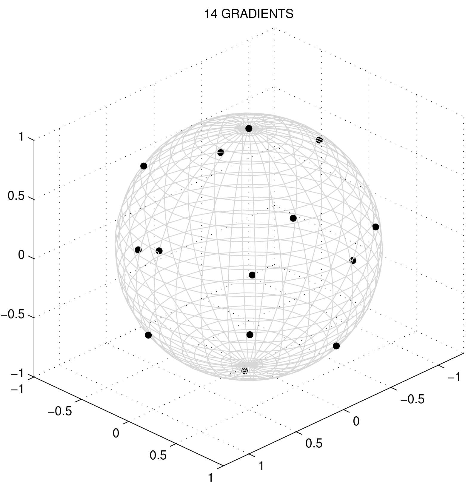
Figure 1: A non-antipodal spherical $t$-design of order 4, with 14 gradients, by Rob Womersley

for all polynomials $f(u_{1},\dots,u_{m})$ of degree $r\leq t$, where $\sigma$ is the uniform probability measure on ${\mathcal{S}}^{m-1}$, and $\#\Upsilon$ is the number of points in $\Upsilon$. In other words, a spherical $t$-design is a quadrature rule on $S^{m-1}$ with constant weights. The algebraic theory behind such designs is deep and beautiful [18], for a recent survey see [4, 1]. In particular, in dimension $m=3$, spherical $t$-designs of order $t\geq 4$ satisfy (50). A database of spherical $t$-designs on ${\mathcal{S}}^{2}$ computed by Rob Womersley is available at his webpage http://web.maths.unsw.edu.au/~rsw/Sphere/EffSphDes/. Table 1 displays the sizes of these designs and Fig. 1 shows a spherical $t$-design of order 4 with 14 gradients from Womersley’s database.

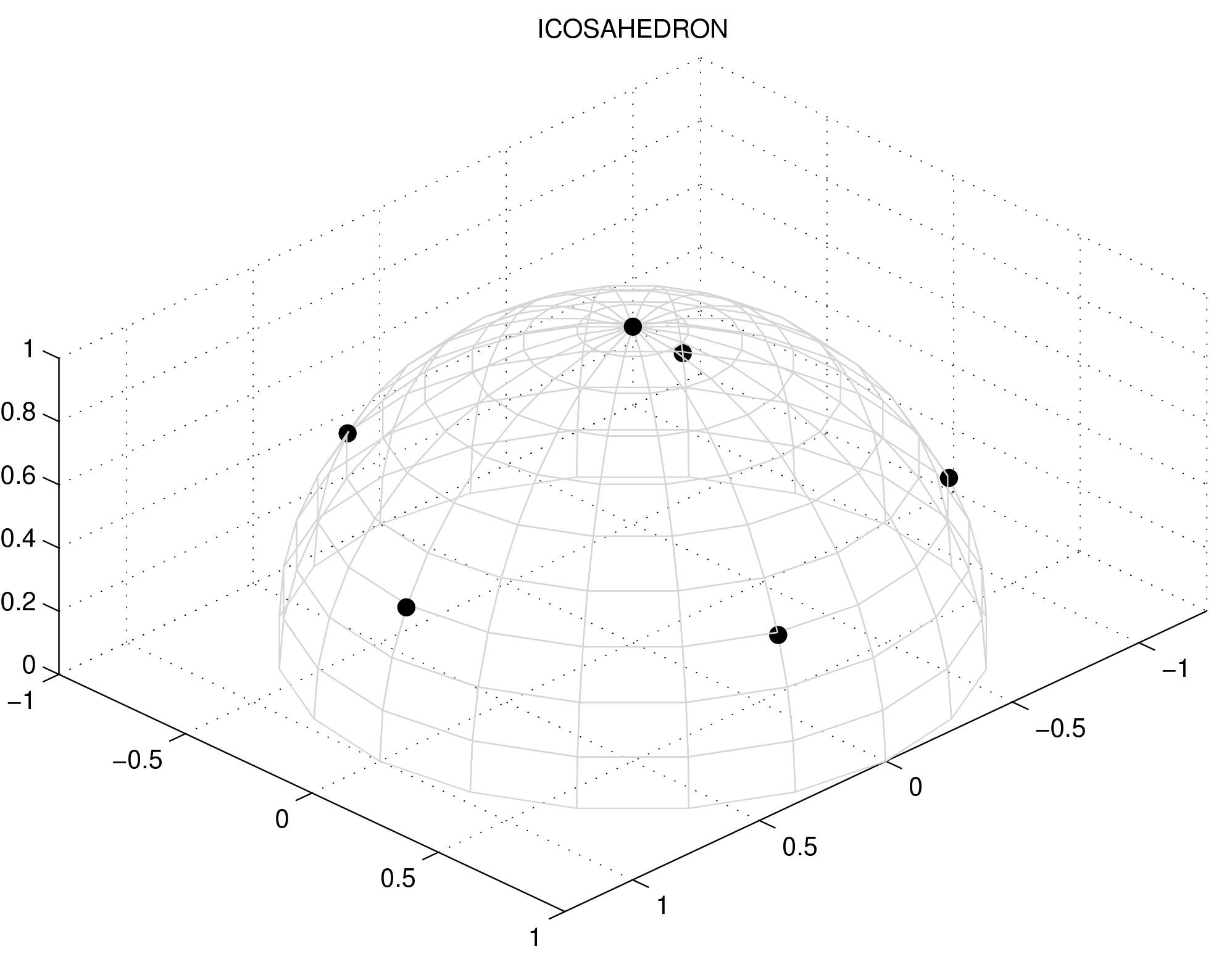
Figure 2: Gradient design based on the icosahedron with 6 gradients on the northern hemisphere.

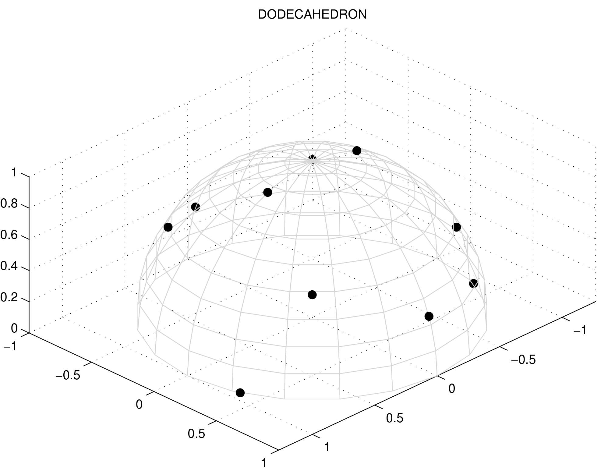
Figure 3: Gradient design based on the dodecahedron with 10 gradients.

When $\Upsilon=-\Upsilon$, we say that the spherical design is antipodal. Two well known examples (see [10],[13]) are the regular icosahedron and its dual, the regular dodecahedron, whose vertices form antipodal spherical $t$-designs of order $5$ with sizes $12$ and $20$, respectively. Note that any two antipodal gradients produce the same DTI-signal. Starting from an antipodal spherical $t$-design $\Upsilon$ and selecting one gradient from each antipodal pair $\{u,-u\}\subset\Upsilon$, we obtain a design $\Upsilon^{\prime}$ of size $\#\Upsilon^{\prime}=\#\Upsilon/2$ which satisfies (53) for all homogeneous polynomials $f$ of even degree $\leq t$. Figures 2-3 show respectively the intersection of the northern hemisphere with the regular icosahedron and dodecahedron, forming gradient designs of size $6$ and $10$ which satisfy (53) for all homogeneous polynomials $f$ of degrees $2$ and $4$.

In the DTI experiment, for a finite subset of $b$-values $0<b_{1}^{(n)}\leq\dots\leq b_{n}^{(n)}$ and respective spherical $t$-designs $\Upsilon_{\ell}^{(n)}$ of order $t^{(n)}_{\ell}\geq 4$, we construct the gradient set as the union of shells

$$G^{(n)}=\bigcup_{\ell=1}^{n}\Upsilon_{\ell}^{(n)}\sqrt{b_{\ell}^{(n)}}\subset\mathbb{R}^{3}\;.$$

The resulting gradient distribution

$$\pi^{(n)}(B)=\frac{\#\bigl{(}G^{(n)}\cap B\bigr{)}}{\#G^{(n)}},\quad B\subseteq\mathbb{R}^{3}\;.$$

satisfies (49), and when the true tensor $\bar{D}=\bar{\gamma}\mbox{I}$ is totally symmetric, we have

$$J^{(n)}(\bar{D})=\bar{\mu}^{(n)}A(1,1)$$

with

$$\bar{\mu}^{(n)}=\frac{1}{15\#G^{(n)}}\sum_{\ell=1}^{n}w\bigl{(}\exp\bigl{(}-\bar{\gamma}b^{(n)}_{\ell}\bigr{)}\rho/\eta\bigr{)}\#\Upsilon^{(n)}_{\ell}\;,$$

i.e. the Fisher information coincides with the precision matrix of an Isotropic Gaussian matrix distribution. When $\Upsilon\subset S^{2}$ is a spherical $t$-design and $O\in SO(3)$ is a rotation matrix, the rotated design $O\Upsilon$ is a spherical $t$-design as well. Since the true tensor $\bar{D}$ is unknown, and possibly it is not isotropic, in practice it is advisable to choose the gradient directions covering ${\mathcal{S}}^{2}$ as uniformly as possible. To achieve that, different $t$-designs can be rotated with respect to each other in order maximize the spread between gradient directions. Namely, starting from a collection of spherical $t$-designs $\Upsilon_{1}^{0},\dots,\Upsilon_{n}^{0}$ of respective orders $t_{k},\;1\leq k\leq n$ we find the optimized design $\Upsilon_{k}^{(n)}=O^{*}_{k}\Upsilon_{k}^{0}$, $1\leq k\leq n$, where $O^{*}_{1},\dots,O^{*}_{n}$ are rotation matrices maximizing

(54) $$\max_{O_{1},\dots,O_{n}\in SO(3)}\min_{1\leq k<l\leq n}\bigl{\{}\mbox{dist}(O_{k}\Upsilon^{0}_{k},O_{l}\Upsilon_{l}^{0})\bigr{\}}\;,$$

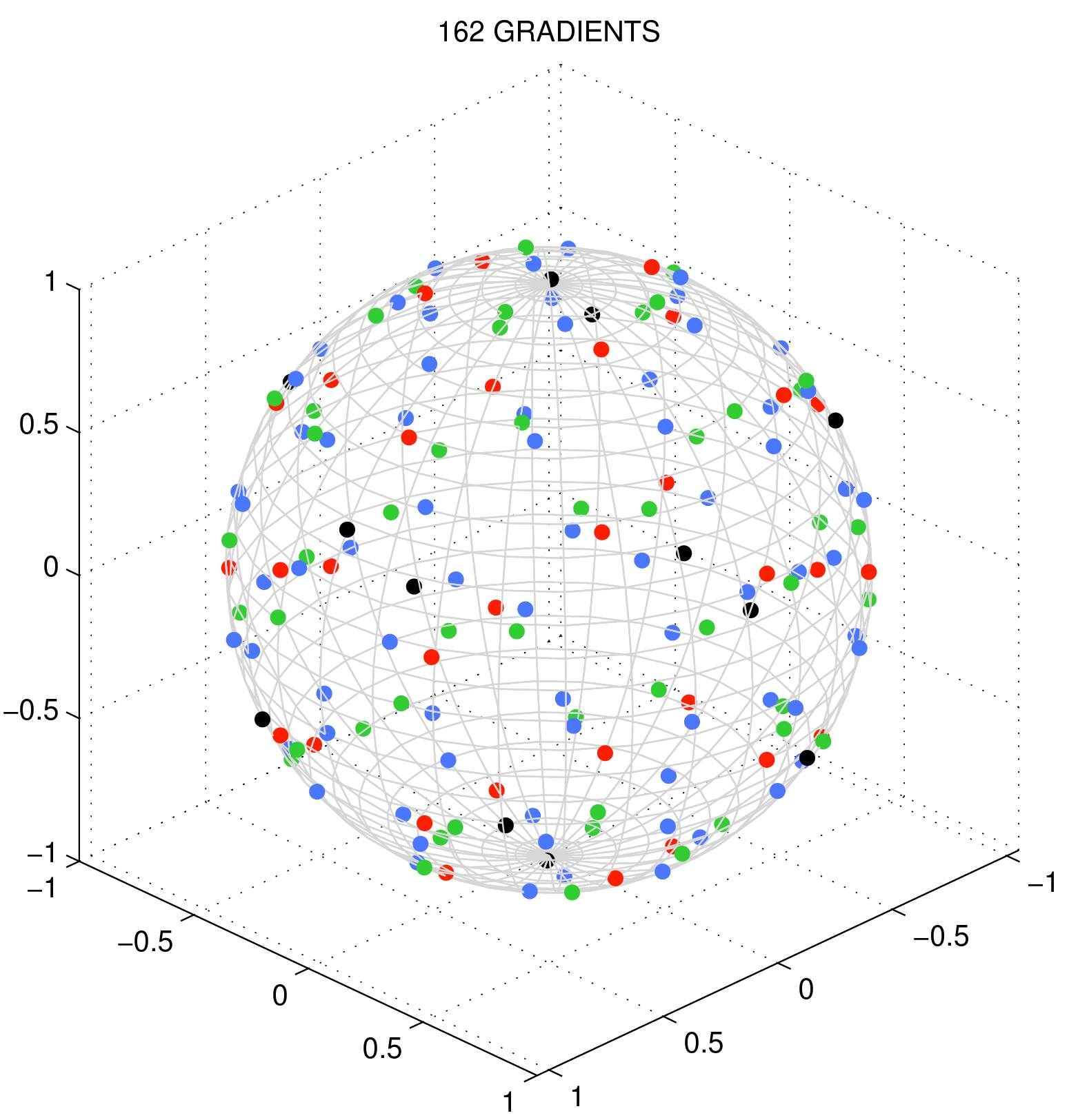
Figure 4: Gradient sequence based on combined antipodal spherical $t$-designs of orders 5 (black),7 (red),9 (green) and 11 (blue), of respective sizes 12,32,48 and 70. The spherical $t$-designs on different shells were rotated in order to maximize the minimal geodesic distance (54) between gradients.

with $\mbox{dist}(U,V)=\sup_{ u\in U,v \in V}\mbox{dist}(u,v)$ and $\mbox{dist}(u,v)$ is the geodesic distance on  ${\mathcal{S}}^{2}$. This can be achieved by a greedy iterative algorithm, where in turn (54) is optimized with respect to each single $O_{k}$ keeping fixed the other rotations until convergence to a fixed point. Fig. 4 shows a gradient sequence obtained in such a way, with colors correponding to spherical $t$-designs on different shells. The benefits of these gradient designs are illustrated in the next paragraph.

7 ILLUSTRATION OF THE METHODS

7.1 Monte Carlo study with isotropic Gaussian noise

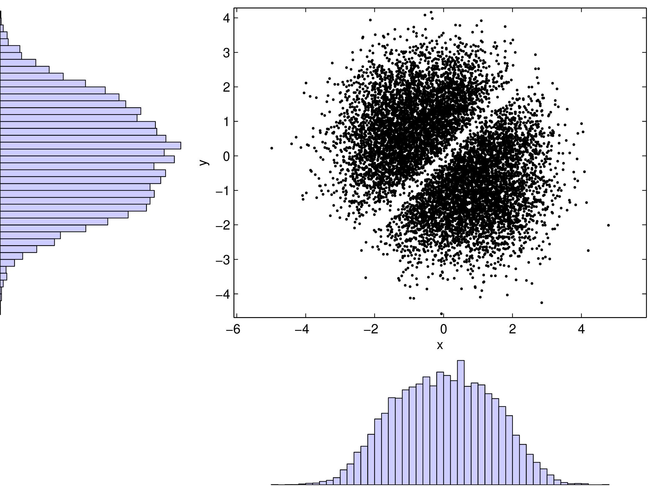
(a) $\{\gamma_{i},\gamma_{j}\},1\leq i\neq j\leq 3$, $\bar{\gamma}_{i}=0$.

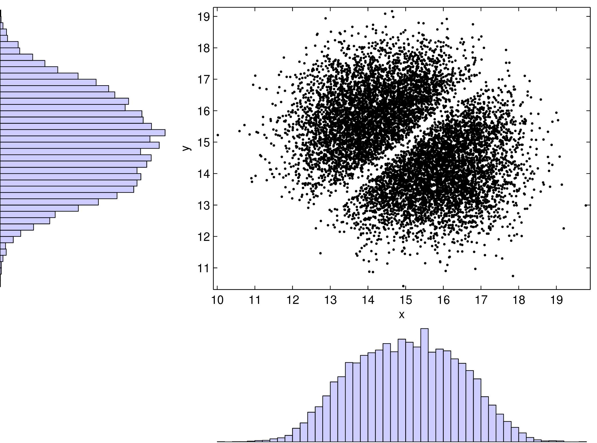
(b) $\{\gamma_{i},\gamma_{j}\},1\leq i\neq j\leq 3$, $\bar{\gamma}_{1}=\bar{\gamma}_{2}=\bar{\gamma}_{3}=15$.

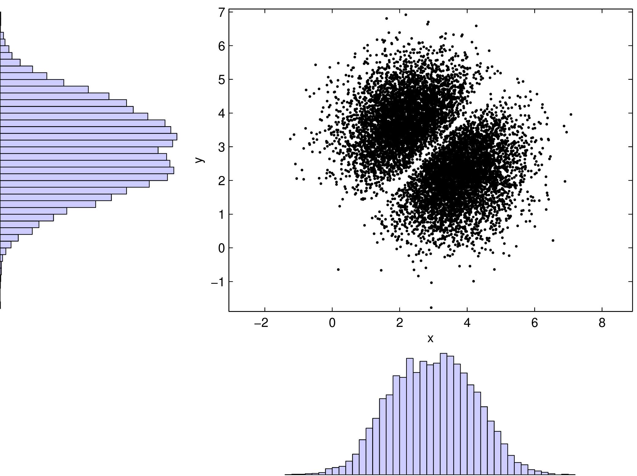
(c) $\{\gamma_{2},\gamma_{3}\}$,$\bar{\gamma}_{1}=15>\bar{\gamma}_{2}=\bar{\gamma}_{3}=3$ .

(d) $\{\gamma_{1},\gamma_{2}\}$, $\bar{\gamma}_{1}=15=\bar{\gamma}_{2}=15>\bar{\gamma}_{3}=3$.

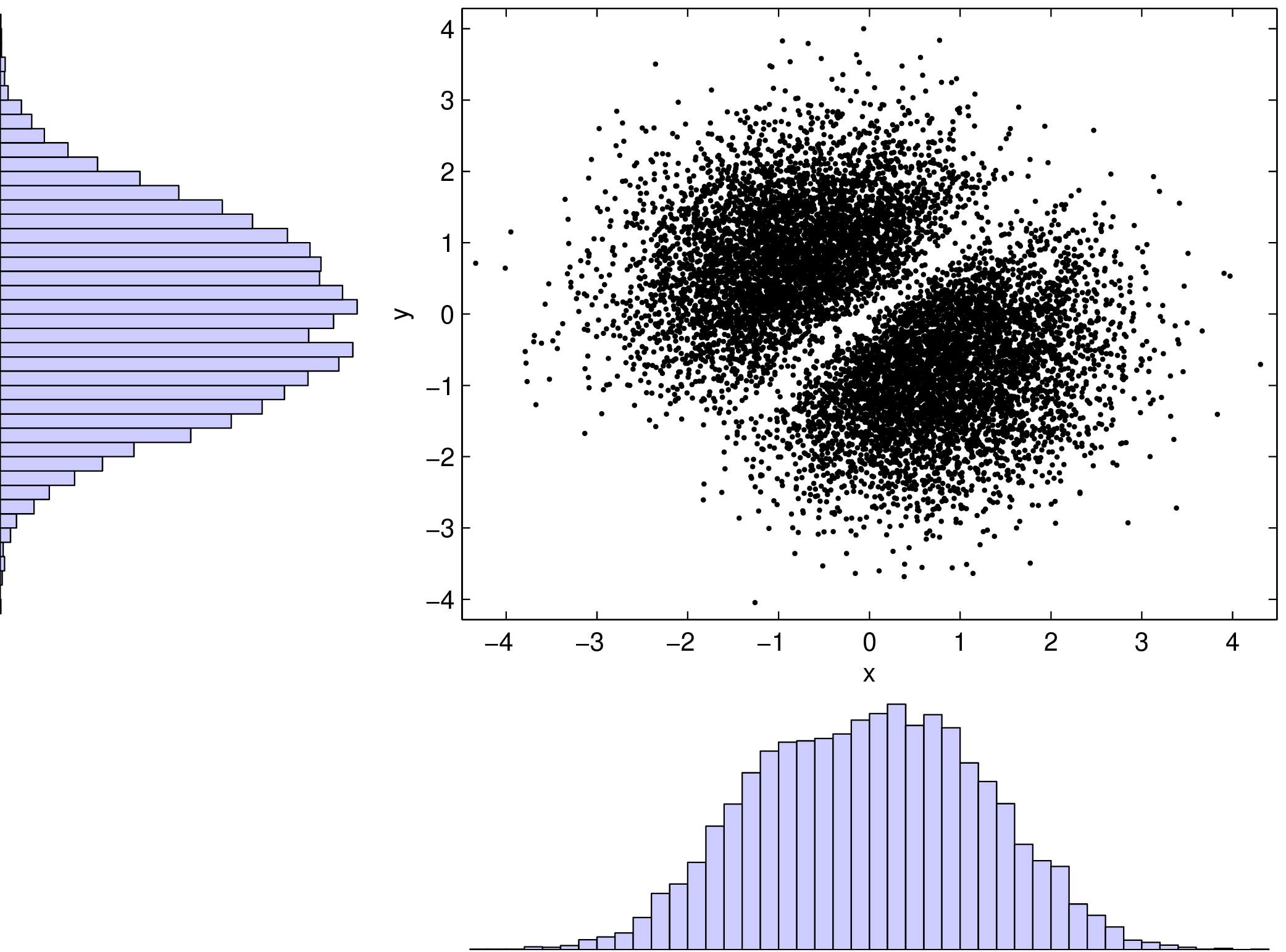
(e) $2\times 2$-GOE eigenvalues

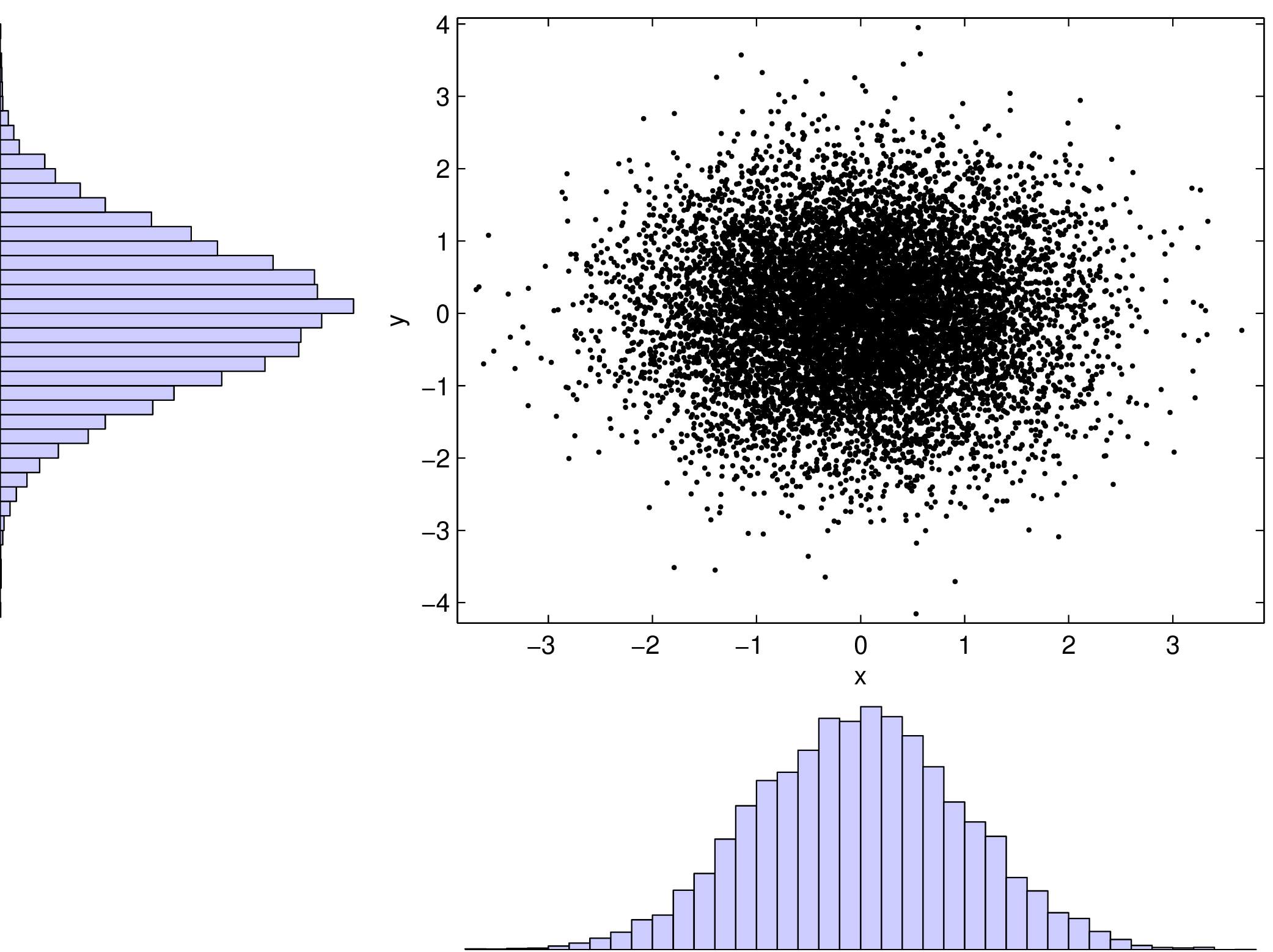
(f) i.i.d. standard Gaussian pairs

Figure 5: $10000$ pairs of distinct eigenvalues of i.i.d. symmetric random matrices with isotropic Gaussian noise ($\mu=1/2$, $\lambda=0$) with various mean: zero, corresponding to the $3\times 3$-GOE (a),isotropic (b), prolate (c), oblate (d). For comparison we show i.i.d. $2\times 2$-GOE eigenvalue pairs (e), and i.i.d. standard Gaussian pairs (f). Within each pair the ordering is randomized, to emphasize the repulsion effect around the diagonal.

Fig. 5 shows the results from a Monte Carlo study with a sample of $N=10000$ i.i.d. $3\times 3$ symmetric random matrices with isotropic Gaussian density (1) with precision parameters $\mu=1/2$, $\lambda=0$, for various choices of the diagonal mean matrix:

1. $\bar{D}=0$, correponding to the $3\times 3$ GOE,

2. $\bar{D}$ isotropic, with $\bar{\gamma}_{1}=\bar{\gamma}_{2}=\bar{\gamma}_{3}=15$,

3. $\bar{D}$ prolate, with $\bar{\gamma}_{1}=15>\bar{\gamma}_{2}=\bar{\gamma}_{3}=3$,

4. $\bar{D}$ oblate, with $\bar{\gamma}_{1}=\bar{\gamma}_{2}=15>\bar{\gamma}_{3}=3$.

For comparison we show in Fig. 5e i.i.d. eigenvalue pairs from the $2\times 2$-Gaussian orthogonal ensemble, and in 5f i.i.d. pairs of independent standard Gaussian random variables. The empirical joint eigenvalue distribution avoids the diagonal, in agreement with (10). We see that the fluctuations of the eigenvalues corresponding to the same $\bar{D}$ eigenspaces around their mean are distributed like the GOE corresponding to the dimension of the eigenspace. One can see also some differences between the GOE eigenvalue distribution in dimension 2 (in Fig. 5e, sampled with precision parameters $\mu=1/2,\lambda=0$, which agrees with 5(c) and 5(d)), and dimension 3 (in Fig. 5(a), which agrees with 5(b)).

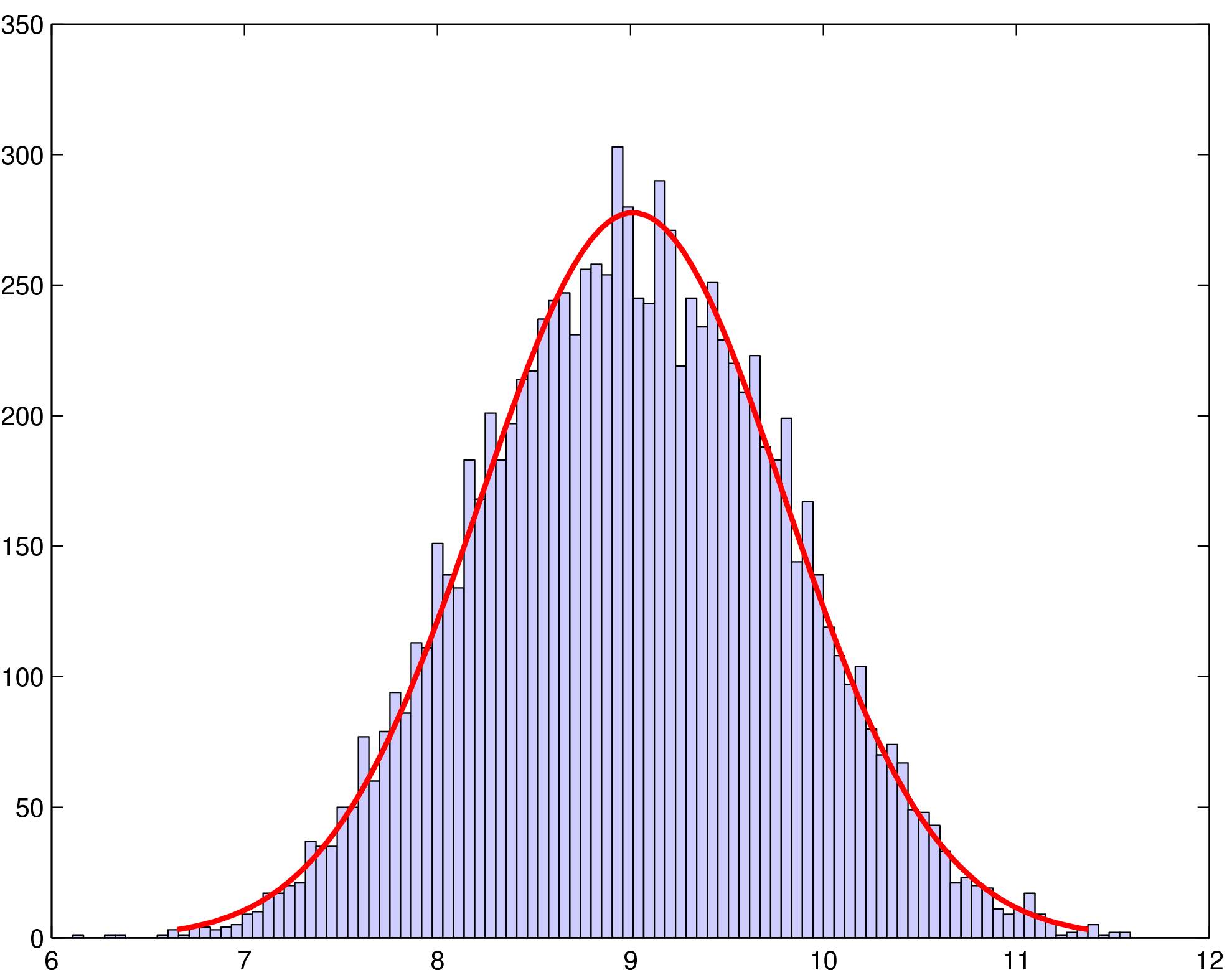
Figure 6: Histogram and fitted Gaussian curve from 10000 i.i.d. realizations of the cluster barycenter $(\gamma_{2}+\gamma_{3})/2$, in the prolate mean tensor case.

Fig. 6 shows that, in the case with prolate mean matrix, the empirical distribution of the cluster barycenter $(\gamma_{2}+\gamma_{3})/2$ fits very well the Gaussian distribution.

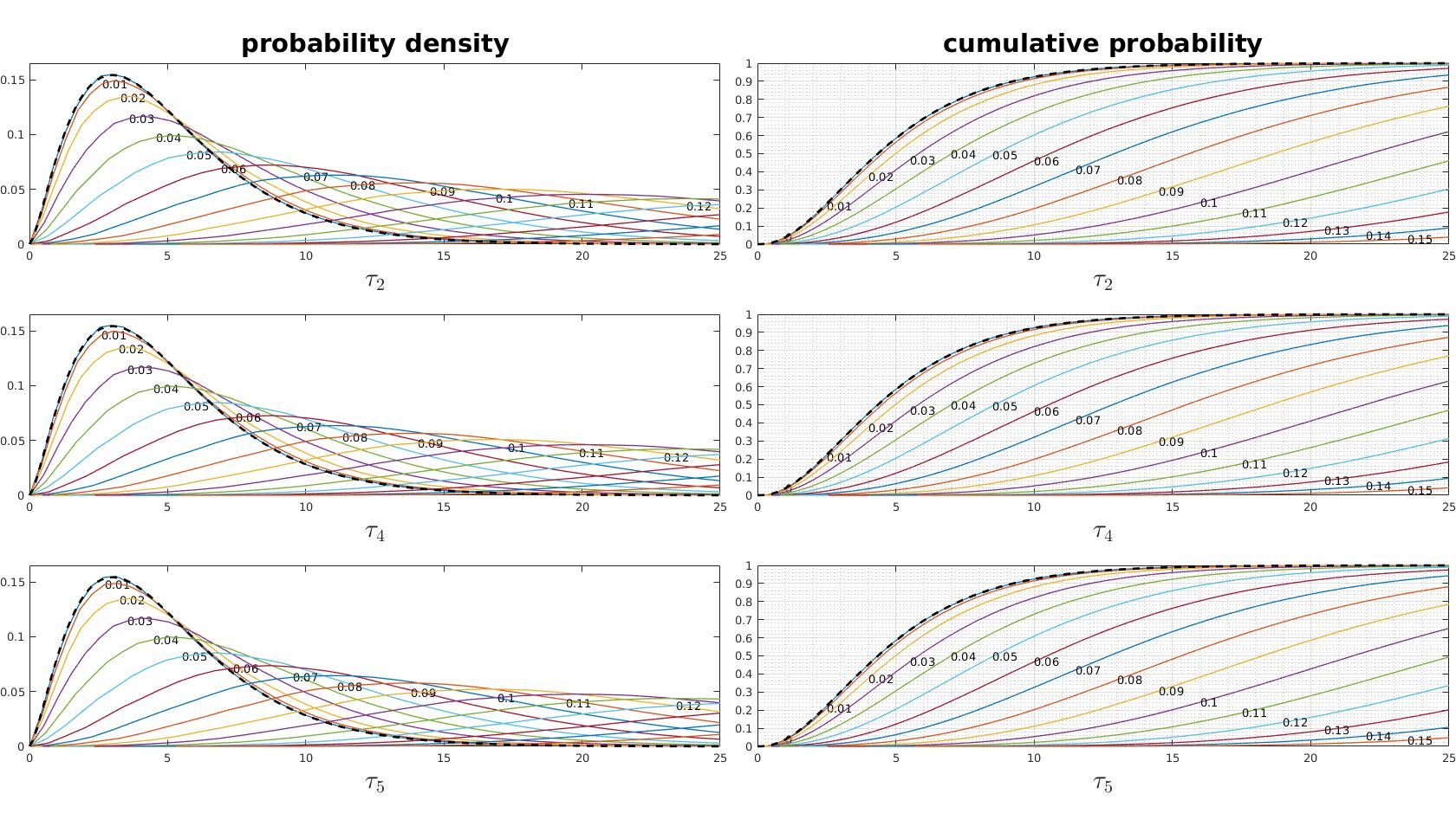
Figure 7: Probability densities (left) and cumulative probabilities (right) of the sphericity test statistics $\tau_{2}(D),\tau_{4}(D),\tau_{5}(D)$, where the $3\times 3$ symmetric random matrix $D$ is Gaussian with isotropic precision $A(2,2)$, and there are $16$ alternative mean tensors $\bar{D}$, with fixed mean diffusivity $\kappa_{1}(\bar{D})=15$. Under the null hypothesis $\bar{D}$ is spherical, while the alternatives correspond to prolate mean tensors with FA in $(0.0,0.15]$. For each test statistics, the probability density and cumulative probability curves are labeled by the FA values of the corresponding mean tensors. The broken curves display the $\chi^{2}_{5}$ limit distribution under the null hypothesis.

Fig. 7 shows the behaviour of the sphericity test statistics $\tau_{2},\tau_{4},\tau_{5}$ under Gaussian matrix distributions with the same isotropic precision matrix $A(2,2)$, and different means: namely a spherical mean tensor, and $15$ prolate mean tensors, all with the same mean diffusivity $\kappa_{1}(\bar{D})=15$, and FA in $(0.01,0.15]$. We can see that at this noise level, under the null hypothesis, the distributions of these three test statistics fit very well the asymptotic $\chi_{5}^{2}$ distribution, while under prolate alternatives the corresponding sphericity tests have approximately the same power at all significance levels.

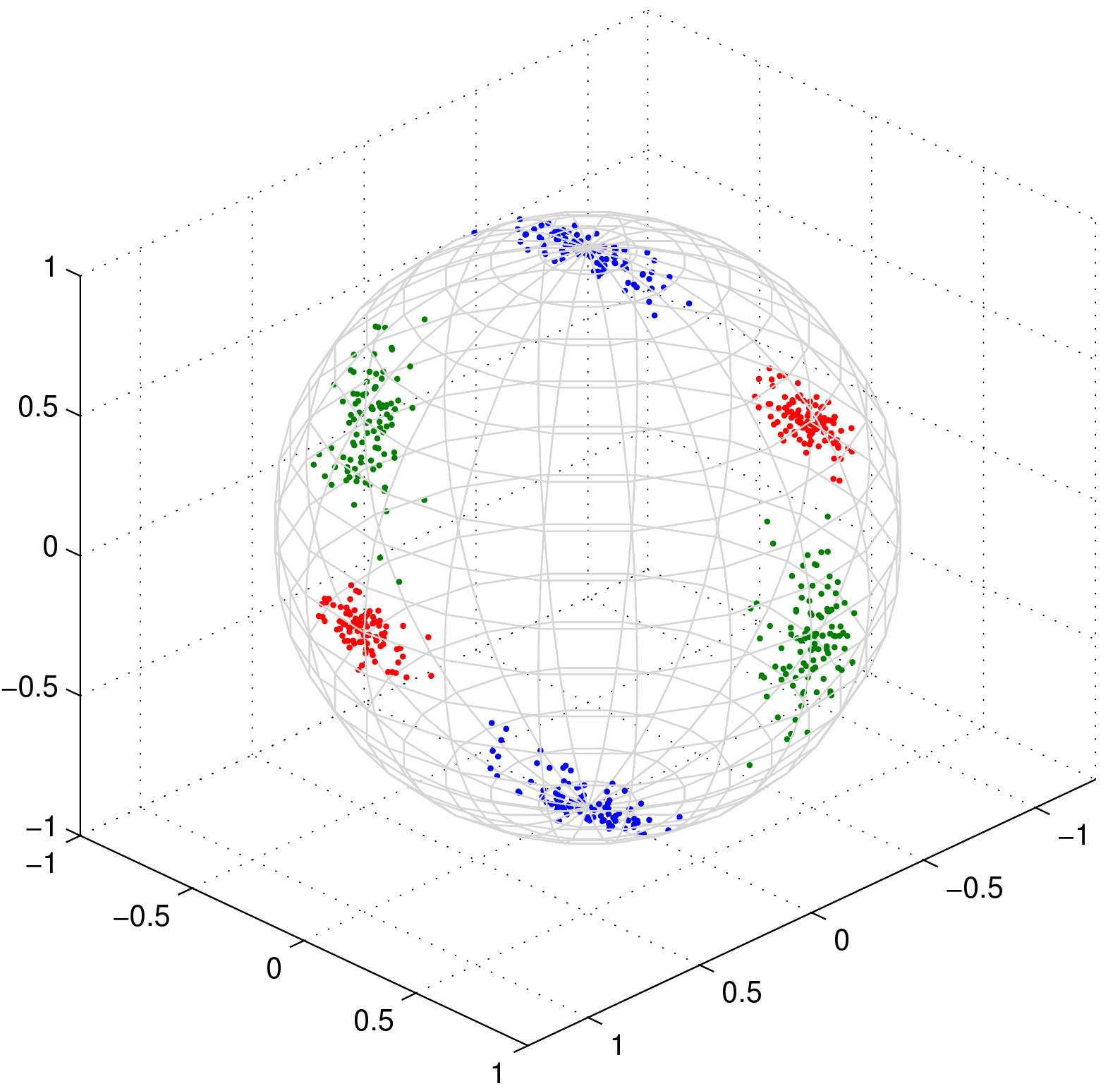
(a) $\bar{\gamma}_{1}=15,\bar{\gamma}_{2}=7.5,\bar{\gamma}_{3}=3$.

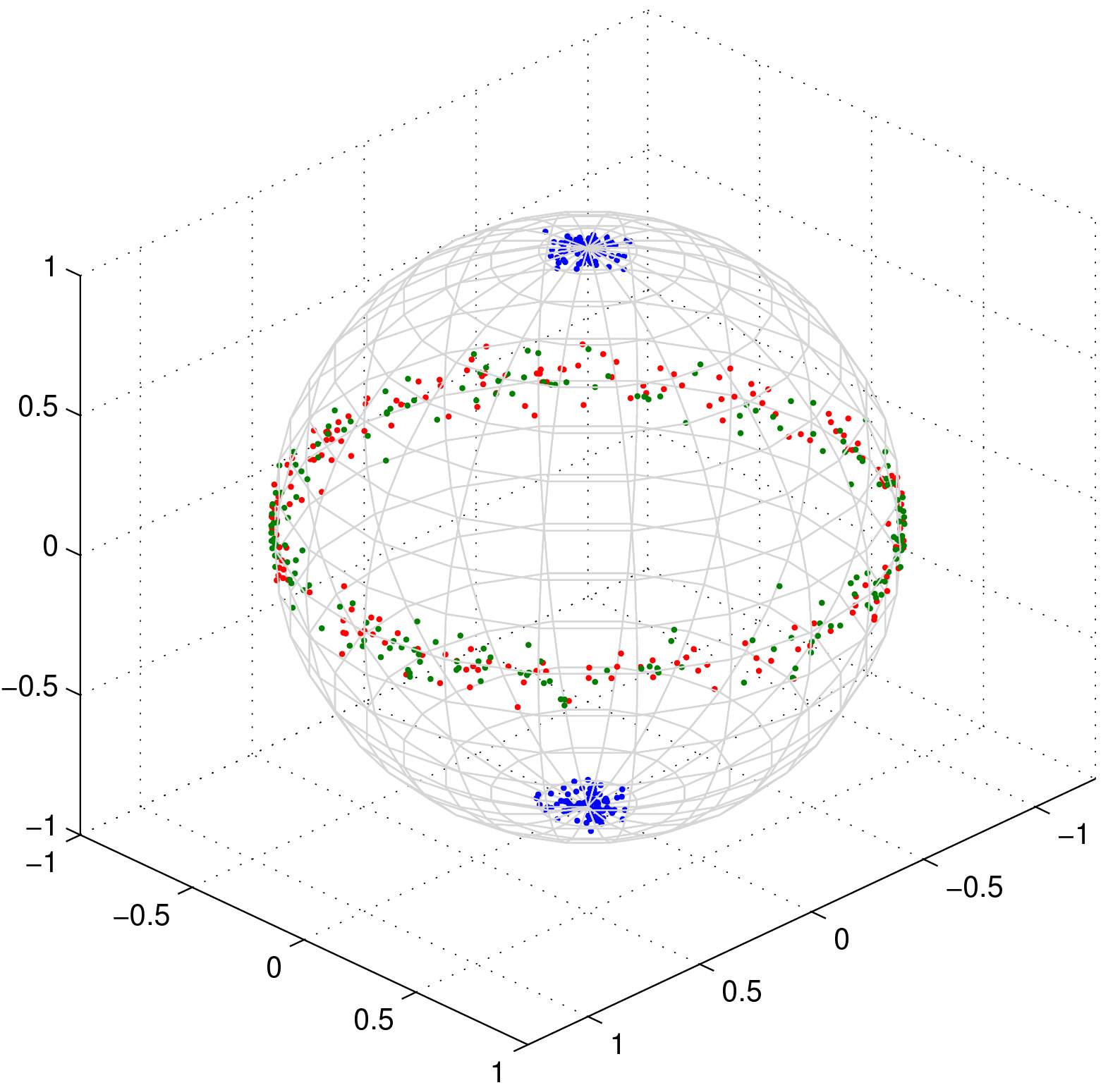
(b) $\bar{\gamma}_{1}=\bar{\gamma}_{2}=15,\bar{\gamma}_{3}=3$.

Figure 8: 200 i.i.d. orthonormal eigenvector triples from the Gaussian model with isotropic noise parameters $\mu=1/2,\lambda=0$, with totally asymmetric (left) and oblate (right) diagonal mean tensor, using a similar graphical construction as the one introduced in [9].

Fig. 8(b) displays on the unit sphere the orthonormal eigenvector triples from the Gaussian model with isotropic noise parameters $\mu=1/2,\lambda=0$, with $N=200$ i.i.d. replications. On the left side figure the mean tensor diagonal and totally anisotropic with $\bar{\gamma}_{1}=15,\bar{\gamma}_{2}=7.5,\bar{\gamma}_{3}=3$. On the right the mean tensor is diagonal and oblate, with $\bar{\gamma}_{1}=\bar{\gamma}_{2}=15,\bar{\gamma}_{3}=3$, and the eigenvectors corresponding to the first two eigenvalues are uniformly distributed around the equator.

7.2 Monte Carlo study of sphericity test statistics based on DTI data with Rician noise

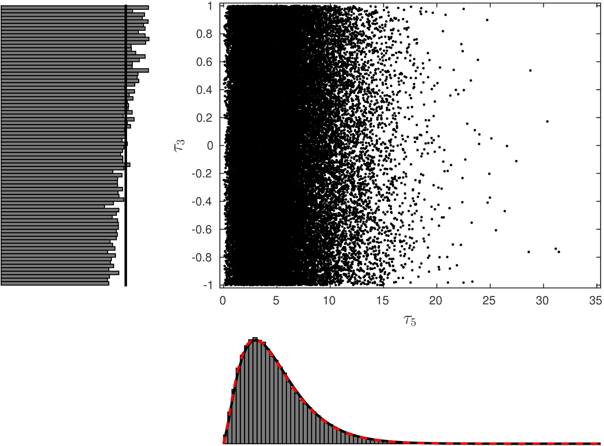
(d)

Figure 9: Scatterplot of the eigenvalue statistics $(\tau_{2}^{(n)},|\tau_{3}^{(n)}|)$ in (a) and $(\tau_{5}^{(n)},\tau_{3}^{(n)})$ in (b), from a Monte Carlo study based on $N=50000$ replications of a dataset generated under Design 1, where the true tensor and the Fisher information are isotropic. The histogram density estimators are compared with theoretical limit densities (black continuous curves), which are uniform on the vertical axes and $\chi^{2}_{5}$ on the horizontal axes. The best fitting gamma densities (red broken curves) are also shown, with shape parameter $2.4238$ and scale parameter $2.0627$ in (a) and with shape parameter $2.4566$ and scale parameter $2.0137$ in (b).

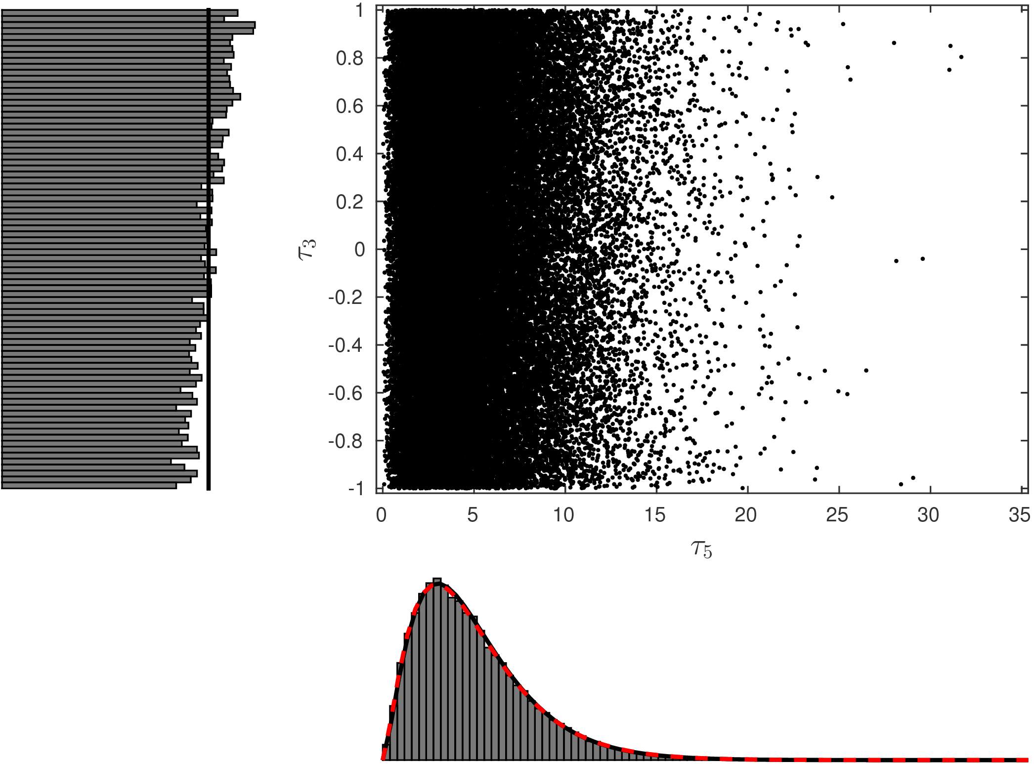
(b)

Figure 10: Scatterplot of the eigenvalue statistics $(\tau_{2}^{(n)},|\tau_{3}^{(n)}|)$ in (a) and $(\tau_{5}^{(n)},\tau_{3}^{(n)})$ in (b), from a Monte Carlo study based on $N=50000$ replications of a dataset generated under Design 2, where the true tensor and the Fisher information are isotropic. The histogram density estimators are compared with theoretical limit densities (black continuous curves), which are uniform on the vertical axes and $\chi^{2}_{5}$ on the horizontal axes. The best fitting gamma densities (red broken curves) are also shown, with shape parameter $2.4103$ and scale parameter $2.0842$ in (a) and with shape parameter $2.4315$ and scale parameter $2.0542$ in (b).

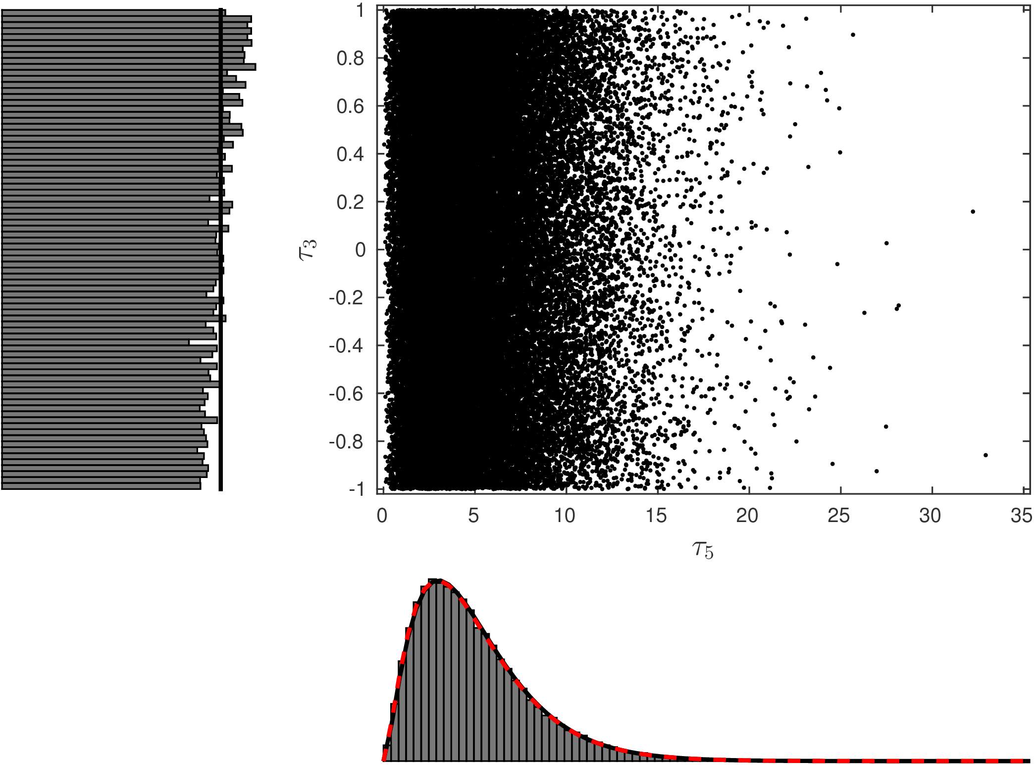
(b)

Figure 11: Scatterplot of the eigenvalue statistics $(\tau_{2}^{(n)},|\tau_{3}^{(n)}|)$ in (a) and $(\tau_{5}^{(n)},\tau_{3}^{(n)})$ in (b), from a Monte Carlo study based on $N=50000$ replications of a dataset generated under Design 3, where the true tensor and the Fisher information are isotropic. The histogram density estimators are compared with theoretical limit densities (black continuous curves), which are uniform on the vertical axes and $\chi^{2}_{5}$ on the horizontal axes. The best fitting gamma densities (red broken curves) are also shown, with shape parameter $2.4405$ and scale parameter $2.0467$ in (a) and with shape parameter $2.4526$ and scale parameter $2.0298$ in (b).

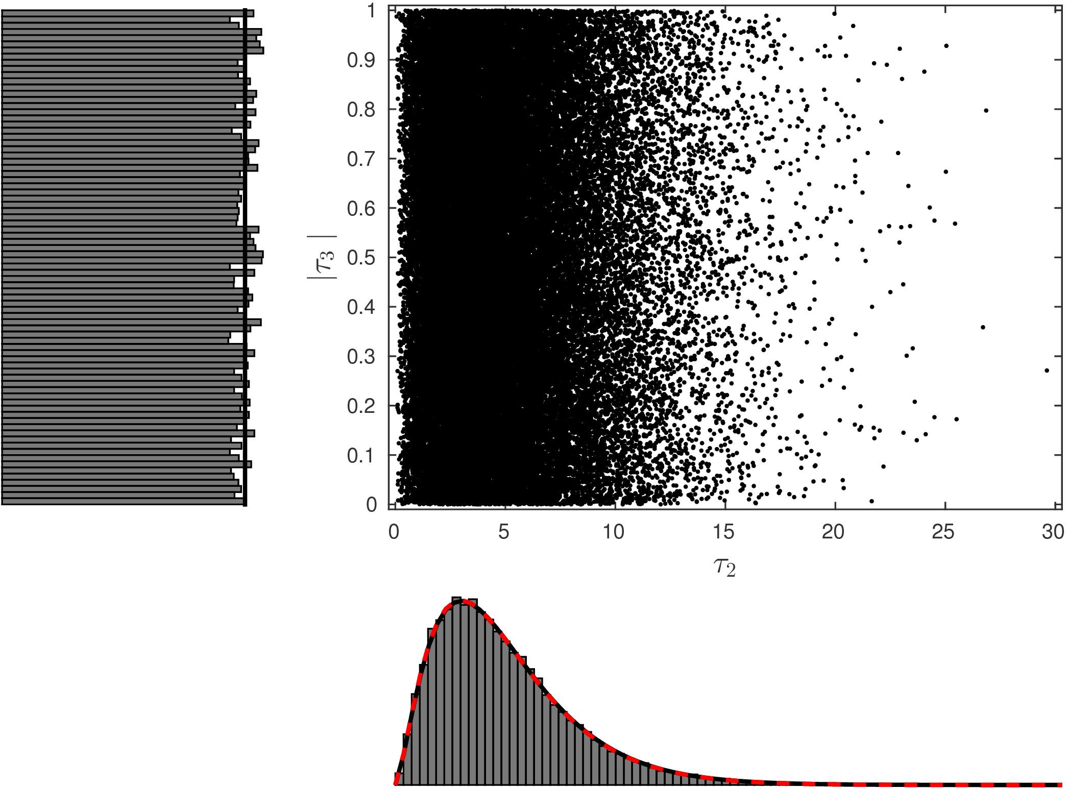
(a)

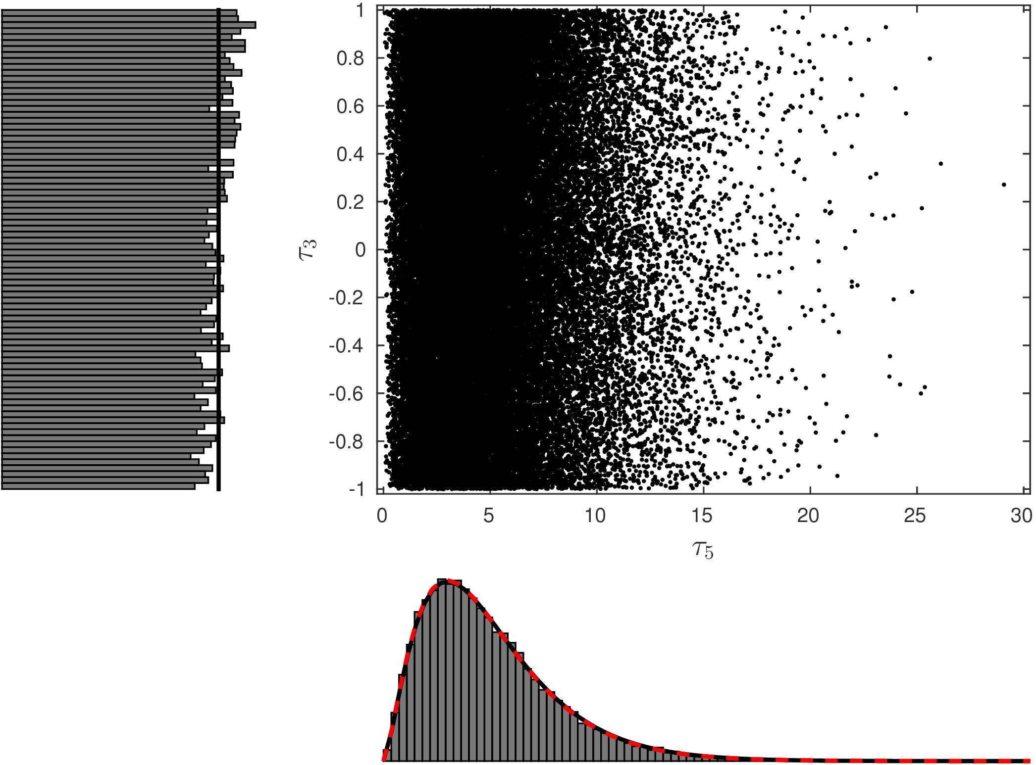
(b)

Figure 12: Scatterplot of the eigenvalue statistics $(\tau_{2}^{(n)},|\tau_{3}^{(n)}|)$ in (a) and $(\tau_{5}^{(n)},\tau_{3}^{(n)})$ in (b), from a Monte Carlo study based on $N=50000$ replications of a dataset generated under Design 4, where the true tensor and the Fisher information are isotropic. The histogram density estimators are compared with theoretical limit densities (black continuous curves), which are uniform on the vertical axes and $\chi^{2}_{5}$ on the horizontal axes. The best fitting gamma densities (red broken curves) are also shown, with shape parameter $2.4924$ and scale parameter $1.9986$ in (a) and with shape parameter $2.4993$ and scale parameter $1.9896$ in (b).

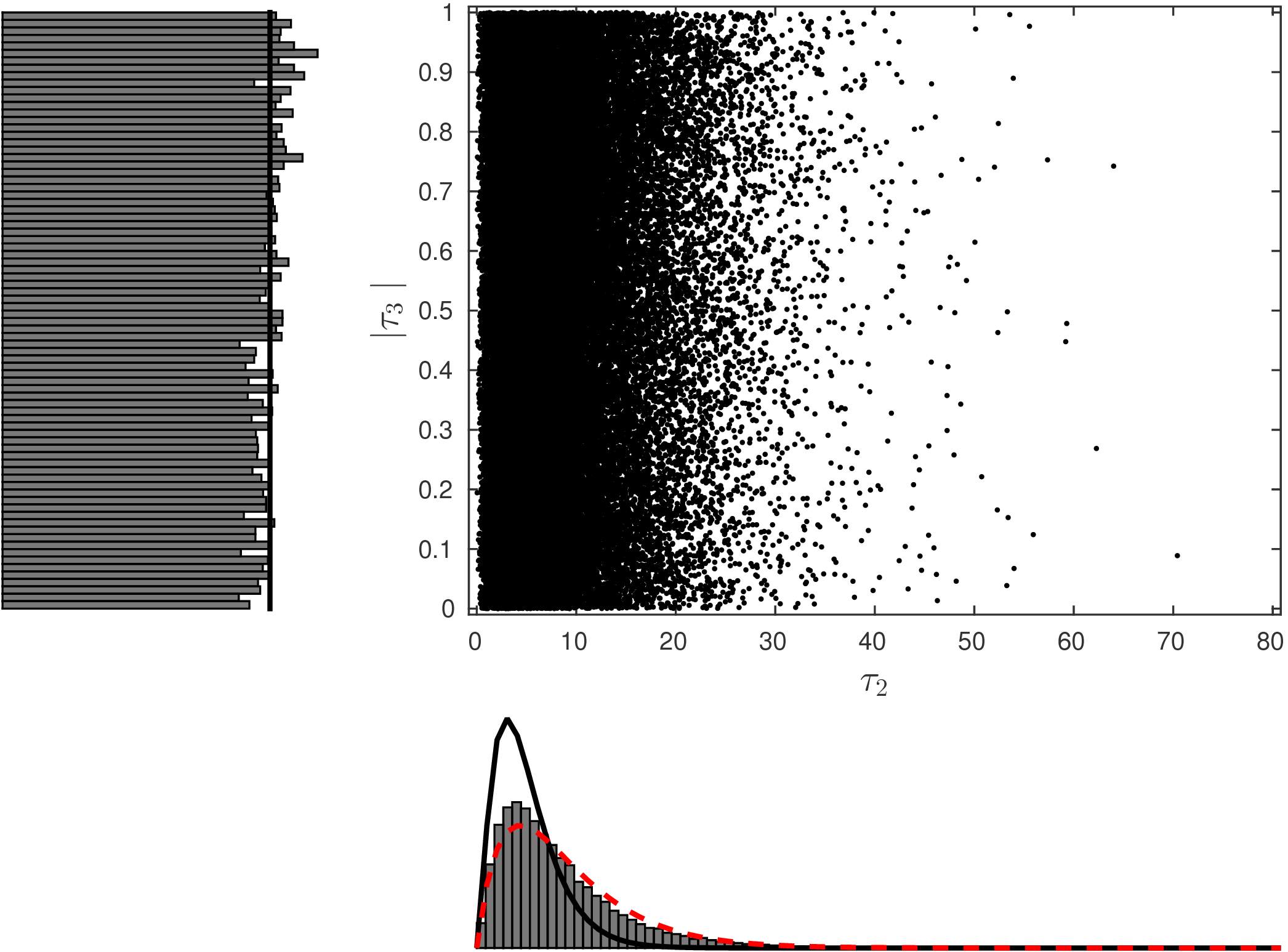
(a)

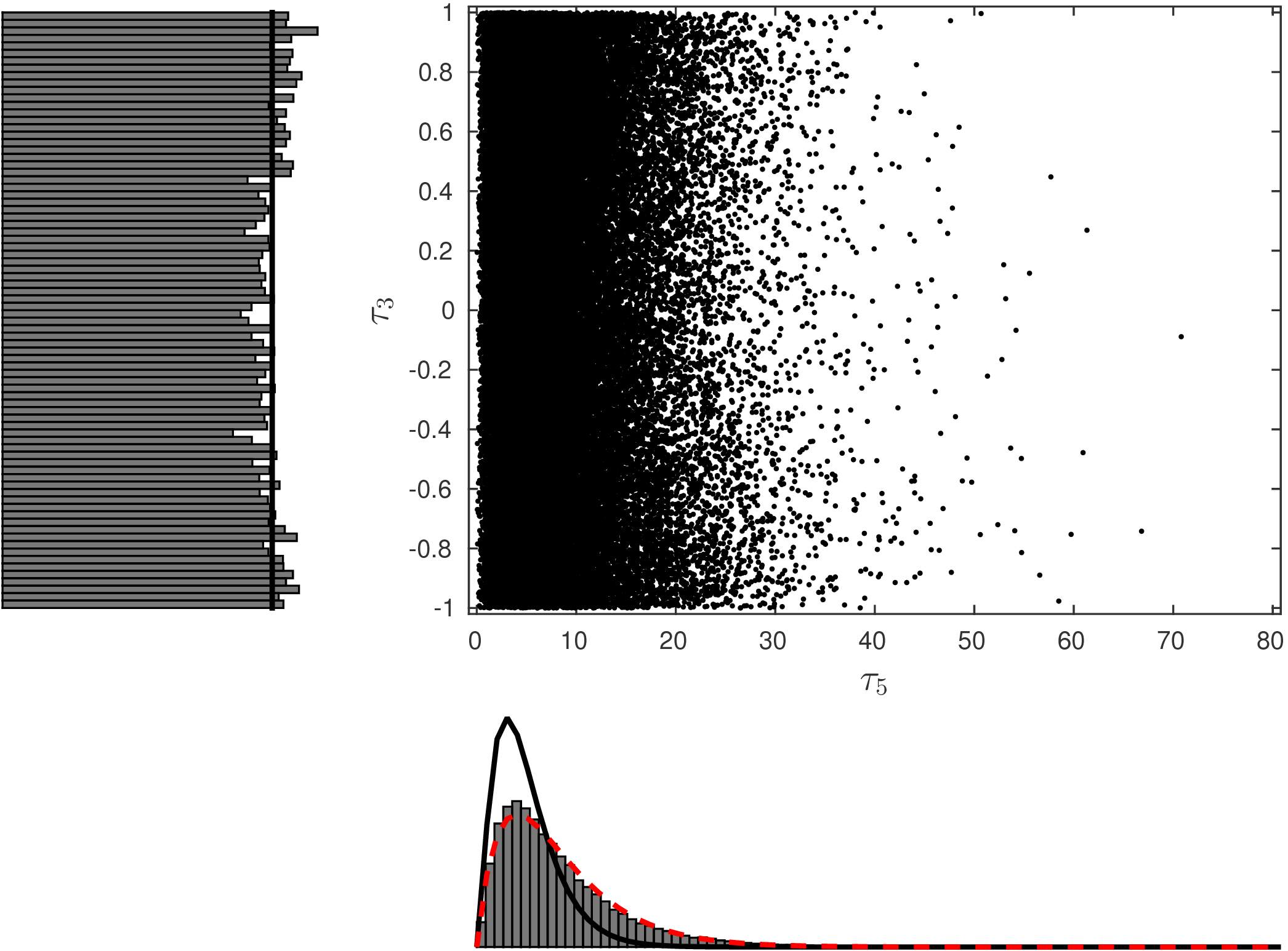
(b)

Figure 13: Scatterplot of the eigenvalue statistics $(\tau_{2}^{(n)},|\tau_{3}^{(n)}|)$ in (a) and $(\tau_{5}^{(n)},\tau_{3}^{(n)})$ in (b), from a Monte Carlo study based on $N=50000$ replications of a dataset generated under Design 5, with isotropic true tensor and anisotropic Fisher information. The histogram density estimators are compared with theoretical limit densities (black continuous curves), which are uniform on the vertical axes and $\chi^{2}_{5}$ on the horizontal axes. The best fitting gamma densities (red broken curves) are also shown, with shape parameter $1.9576$ and scale parameter $4.5494$ in (a) and with shape parameter $1.9565$ and scale parameter $4.2094$ in (b).

In order to validate the asymptotic results of Lemma 5.4 and Corollary 5.6, we conducted another large Monte Carlo study, with DTI data simulated under the Rician noise model with ground truth parameters $\eta^{2}=64.056$, $\rho=110.046$, and isotropic diffusion tensor $\bar{D}=6.622\times 10^{-4}\times\mbox{\rm Id}$ ${\rm mm^{2}/s}$. For each of the experimental designs 1-5 below, which have increasing number of acquisitions, we simulated $N=50000$ replications of the dataset, and for each replication we computed the MLE $D^{(n)}$ based on the simulated data by using the EM-algorithm from [29]. The empirical distribution of the sphericity statistics $\tau_{2}^{(n)},\tau_{3}^{(n)}$ (33) and $\tau_{5}^{(n)}$ (39) with their theoretical limit distributions are displayed correspondingly in Figures 9-13.

1. Spherical $t$-design of order $4$ with $14$ gradients computed by R. Womersley, shown in Fig. 1, with $b$-value $996$ ${\rm s/mm^{2}}$, and one acquisition at zero $b$-value, for a total of $15$ acquisitions. The corresponding Fisher information is given by

   $$J^{(n)}(\bar{D})=\bar{\mu}^{(n)}A_{3}(1,1),\quad\bar{\mu}^{(n)}=4.63\times 10^{7}{\rm s^{2}/{mm^{4}}},$$

   and the ML estimator $\mbox{vec}(D^{(n)})$ has a Gaussian approximation with mean $\mbox{vec}(\bar{D})$ and isotropic covariance

   $$\Sigma^{(n)}=J^{(n)}(\bar{D})^{-1}=10^{-9}\times\left(\begin{matrix}8.64&-2.16&-2.16&0&0&0\\ -2.16&8.64&-2.16&0&0&0\\ -2.16&-2.16&8.64&0&0&0\\ 0&0&0&5.4&0&0\\ 0&0&0&0&5.4&0\\ 0&0&0&0&0&5.4\\ \end{matrix}\right){\rm\frac{mm^{4}}{s^{2}}}\;.$$

2. It is based on the icosahedron with the $6$ gradients shown in Fig. 2 for each $b$-value in the set $\{560,778,996,1276,1556,1898,2240\}$ ${\rm s/mm^{2}}$, and one acquisition at zero $b$-value, for a total of $43$ acquisitions. The corresponding Fisher information is given by

   $$J^{(n)}(\bar{D})=\bar{\mu}^{(n)}A_{3}(1,1),\;\bar{\mu}^{(n)}=1.323\times 10^{8}{\rm s^{2}/{mm^{4}}}$$

   and the ML estimator $\mbox{vec}(D^{(n)})$ has a Gaussian approximation with mean $\mbox{vec}(\bar{D})$ and isotropic covariance

   $$\Sigma^{(n)}=J^{(n)}(\bar{D})^{-1}=10^{-9}\times\left({\small\begin{matrix}3.02&-0.76&-0.76&0&0&0\\ -0.76&3.02&-0.76&0&0&0\\ -0.76&-0.76&3.02&0&0&0\\ 0&0&0&1.89&0&0\\ 0&0&0&0&1.89&0\\ 0&0&0&0&0&1.89\\ \end{matrix}}\right){\rm\frac{mm^{4}}{s^{2}}}\;.$$

3. It is based on the dodecahedron with the $10$ gradients shown in Fig. 3 for each $b$-value in the set

   $$\bigl{\{}560,778,996,1276,1556,1898,2240\bigr{\}}\;{\rm s/mm^{2}},$$

   and one acquisition at zero $b$-value, for a total of $71$ acquisitions. The corresponding Fisher information is given by

   $$J^{(n)}(\bar{D})=\bar{\mu}^{(n)}A_{3}(1,1),\quad\bar{\mu}^{(n)}=2.205\times 10^{8}{\rm s^{2}/{mm^{4}}},$$

   and the ML estimator $\mbox{vec}(D^{(n)})$ has a Gaussian approximation with mean $\mbox{vec}(\bar{D})$ and isotropic covariance

   $$\Sigma^{(n)}=J^{(n)}(\bar{D})^{-1}=10^{-9}\times\left({\small\begin{matrix}1.81&-0.45&-0.45&0&0&0\\ -0.45&1.81&-0.45&0&0&0\\ -0.45&-0.45&1.81&0&0&0\\ 0&0&0&1.13&0&0\\ 0&0&0&0&1.13&0\\ 0&0&0&0&0&1.13\\ \end{matrix}}\right){\rm\frac{mm^{4}}{s^{2}}}\;.$$

4. Combination of spherical $t$-designs of orders 5,7,9,11, shown in Fig. 4 on shells corresponding to the $b$-values $\{560,996,1556,2240\}$, respectively, with one acquisition at zero $b$-value, for a total of $163$ acquisitions.

   The corresponding Fisher information is given by

   $$J(D^{(n)})=\bar{\mu}^{(n)}A_{3}(1,1),\quad\bar{\mu}^{(n)}=5.263\times 10^{8}{\rm s^{2}/{mm^{4}}},$$

   and the ML estimator $\mbox{vec}(D^{(n)})$ has a Gaussian approximation with mean $\mbox{vec}(\bar{D})$ and isotropic covariance

   $$\Sigma^{(n)}=J^{(n)}(\bar{D})^{-1}=10^{-10}\times\left({\small\begin{matrix}7.6&-1.9&-1.9&0&0&0\\ -1.9&7.6&-1.9&0&0&0\\ -1.9&-1.9&7.6&0&0&0\\ 0&0&0&4.75&0&0\\ 0&0&0&0&4.75&0\\ 0&0&0&0&0&4.75\\ \end{matrix}}\right){\rm\frac{mm^{4}}{s^{2}}}\;.$$

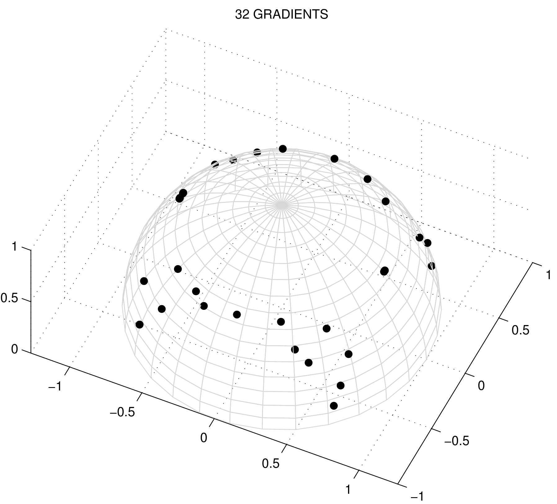
Figure 14: The $32$ gradients table used by default with the commercial 3T Philips Achieva MR-scanner.

5. with $3$ repetitions of the $32$ gradients in Fig. 14 for each $b$-value in

   $$\bigl{\{}\mbox{\footnotesize 62, 249, 560, 996, 1556, 2240, 3049, 3982, 5040 ,6222, 7529, 8960, 10516, 12196, 14000}\bigr{\}}{\rm s/mm^{2}},$$

   and $3$ acquisitions at zero $b$-value, for a total of $1443$ acquisitions. The ML estimator $\mbox{vec}(D^{(n)})$ has a Gaussian approximation with mean $\mbox{vec}(\bar{D})$ and non-isotropic covariance

   (55) $$\Sigma^{(n)}=J^{(n)}(\bar{D})^{-1}=10^{-10}\times\left(\small{\begin{matrix}6.77&-3.24&-2.31&-0.07&-0.08&0.21\\ -3.24&7.04&-2.53&-0.11&0.15&-0.05\\ -2.31&-2.53&6.70&0.10&-0.10&-0.59\\ -0.07&-0.11&0.10&1.17&-0.14&0.01\\ -0.08&0.15&-0.10&-0.14&1.3&-0.01\\ 0.21&-0.05&-0.59&0.01&-0.01&1.33\\ \end{matrix}}\right){\rm\frac{mm^{4}}{s^{2}}}\;.$$

All scatterplots in Figures 9-13 are consistent with the asymptotic independence of the sphericity statistics $\tau_{2}^{(n)}$ and $\tau_{5}^{(n)}$ from $\tau_{3}^{(n)}$. When the experimental design is based on spherical $t$-designs of order $t\geq 4$ (Designs 1-4), with isotropic Fisher information, the empirical distributions of $\tau_{2}^{(n)}$ and $\tau_{5}^{(n)}$ fit well the theoretical limit distribution $\chi^{2}_{5}$ (Figures 9-12). The 5th design has the largest number of acquisitions and it is the most informative of all, however the Fisher information is not isotropic and Fig. 13 shows that the empirical distributions of $\tau^{(n)}_{2}$ and $\tau^{(n)}_{5}$ do not fit the $\chi^{2}_{5}$ distribution, with the consequence of underestimating the Type I error probability of rejecting an isotropic true tensor. We conclude that the distribution of these sphericity statistics is sensitive to anisotropies of the estimation error distribution. As it was shown in section 5, these sphericity test statistics should be calibrated against the law of $\tau(c+\kappa_{1}(X),\kappa_{2}(X),\kappa_{3}(X))$, evaluated at $c=\kappa_{1}(D^{(n)})$, where $X$ is the zero mean symmetric Gaussian matrix with covariance (55).

We also remark that in lower part of Fig. 9-11, compared with the uniform density, the histogram estimator of the $\tau_{3}^{(n)}$ density shows an increasing linear trend. This linear trend is less evident in 12, which is based on a larger number of acquisitions, and the distribution of the MLE $D^{(n)}$ is presumably better approximated by a Gaussian than in the previous cases. By taking absolute value $|\tau_{3}^{(n)}|$ the linear trend cancels out, and the histogram of $|\tau_{3}^{(n)}|$ in the upper part of Figures 9-13 fits robustly the uniform distribution in all the situations we have considered.

8 CONCLUSION

We have considered the problem of estimating the spectrum $\bar{\gamma}_{1}\geq\bar{\gamma}_{2}\geq\dots\geq\bar{\gamma}_{m}$ and the eigenvectors of a real symmetric $m\times m$ matrix $\bar{D}$, possibly non-positive, by the spectrum and the eigenvectors of a consistent and asymptotically Gaussian matrix estimator $D^{(n)}$, assuming that the covariance of the rescaled limit is isotropic. When $\bar{D}$ has repeated eigenvalues, the delta method does not apply and the spectrum of the matrix estimator has a non-Gaussian limit distribution. In the limit, the random eigenvalues $\gamma_{1}^{(n)}>\gamma_{2}^{(n)}>\dots>\gamma_{m}^{(n)}$ of $D^{(n)}$ form clusters corresponding to the $\bar{D}$ eigenspaces, with jointly Gaussian barycenters. Within each cluster, the differences between eigenvalues and barycenter are independent from the barycenter and the other clusters, and follow the conditional law of GOE eigenvalues conditioned on having zero barycenter.

In many applications it is important to detect the symmetries of the true matrix parameter $\bar{D}$, in particular to test whether $\bar{D}$ is spherical, which leads to singular hypothesis testing problems. A statistical test against $\bar{D}$-symmetries needs to be calibrated taking into account the repulsion between the random eigenvalues of $D^{(n)}$ corresponding to the same $\bar{D}$-eigenspace. In dimension $m=3$, we derived the asymptotic joint distribution of some commonly used sphericity statistics as Fractional Anisotropy, Relative Anisotropy and Volume Ratio under isotropy assumptions. We have also discussed the implications of these general results for the design and analysis of DTI measurements, and we showed that gradient designs based on spherical $t$-designs have isotropic Fisher information and are asympotically most informative when the true tensor is spherical. A direct application would be in denoising the FA maps derived from diffusion tensor estimates. Testing for sphericity at each volume element with a fixed confidence level, corresponds to a FA cut-off threshold which is not constant over the voxels but depends locally on the estimated noise and mean diffusivity parameters. We have seen in the Monte Carlo study that the simulated sphericity statistics fit well their theoretical limit distribution when the Fisher information of the experiment was isotropic. However, there was a significant discrepancy under experimental design 5, with non-isotropic Fisher information. We conclude that these findings give a strong theoretical argument in favour of using spherical $t$-designs in DTI, and we plan to conduct similar experiments with real DTI data in the near future. Finally, our work in progress is to generalize this theory to situations in which the covariance of the Gaussian limit matrix has symmetries without being fully isotropic.

Size of Spherical $t$-Designs

$t$	4	5	6	7	8	9	10	11	12	13	14	15	16	17
$n_{a}$	-	12	-	32	-	48	-	70	-	94	-	120	-	156
$n$	14	18	26	32	42	50	62	72	86	98	114	128	146	163

Table 1: Number $n_{a}$ of points in some known antipodal spherical $t$-designs of order $4\leq t\leq 17$ in ${\mathcal{S}}^{2}$, computed by Rob Womersley, while $n$ is for his non-antipodal spherical $t$-designs.

$u_{x}$	$u_{y}$	$u_{z}$
0.0000	0.0000	1.0000
0.9473	0.0000	0.3202
-0.9035	0.1944	-0.3821
0.2693	0.7379	0.6189
0.4465	-0.6627	0.6012
-0.8205	-0.0749	0.5668
-0.1166	0.8072	-0.5787
0.6831	0.6942	-0.2269
0.0897	0.0476	-0.9948
0.7740	-0.2872	-0.5642
0.2389	-0.9284	-0.2846
-0.5595	-0.5216	-0.6441
-0.5094	-0.8054	0.3029
-0.5394	0.7991	0.2655

$u_{x}$	$u_{y}$	$u_{z}$
0.0000	0.0000	1.0000
0.8944	0.0000	0.4472
0.2764	-0.8507	0.4472
-0.7236	0.5257	0.4472
-0.7236	-0.5257	0.4472
0.2764	0.8507	0.4472

$u_{x}$	$u_{y}$	$u_{z}$
-0.9342	0.3568	0.0000
-0.5774	-0.5774	0.5774
-0.5774	0.5774	0.5774
-0.3568	0.0000	0.9342
0.0000	-0.9342	0.3568
0.0000	0.9342	0.3568
0.3568	0.0000	0.9342
0.5774	-0.5774	0.5774
0.5774	0.5774	0.5774
0.9342	0.3568	0.0000

Design 1, sphericity statistics.

(c)

Design 2, sphericity statistics.

(a)

Design 3, sphericity statistics.

(a)

Design 4, sphericity statistics.

Design 5, sphericity statistics.

$u_{x}$	$u_{y}$	$u_{z}$	$u_{x}$	$u_{y}$	$u_{z}$
-0.5000	-0.7071	0.5000	0.7071	-0.5261	0.4725
-0.5000	0.7071	0.5000	-0.7071	-0.0002	0.7071
0.7071	-0.0000	0.7071	-0.7071	0.5261	0.4725
-0.6533	-0.7071	0.2706	0.7071	0.5261	0.4725
-0.2087	-0.7071	0.6756	0.4725	0.5261	0.7071
0.0197	-0.7071	0.7068	-0.7071	0.0078	0.7071
0.4212	-0.7071	0.5679	-0.6364	0.6436	0.4252
0.6899	-0.7071	0.1549	-0.7060	0.0547	0.7060
-0.6535	-0.7069	0.2707	-0.2929	0.6436	0.7071
-0.2929	-0.6436	0.7071	0.2929	0.6436	0.7071
0.2945	-0.6436	0.7064	0.7071	0.0078	0.7071
0.5150	-0.7061	0.4861	0.7071	0.6436	0.2929
0.7071	-0.6436	0.2929	-0.7063	0.0489	0.7063
-0.7071	-0.5261	0.4725	0.0347	0.7071	0.7063
-0.4725	-0.5261	0.7071	0.7071	0.0115	0.7071
0.5555	-0.5261	0.6439	0.7071	0.7071	0.0000

9 APPENDIX

9.1 Proof of Theorems 4.1,4.5,4.6

We follow the line of proof of Theorem 3.1 in [14], (see also [33]), which deals with the eigenvalues of rescaled Wishart random matrices with growing degrees of freedom, and we generalize it to the case of random matrices with asymptotically isotropic Gaussian noise, without the positivity assumption. By Schéffe’s theorem (see [42]), to prove convergence in distribution it is enough to show pointwise almost sure convergence of the densities to a probability density, and we achieve that by using Laplace approximation. Note first that when the mean matrix $\bar{D}$ is isotropic with equal eigenvalues $\bar{\gamma}_{1}=\bar{\gamma}_{2}=\dots=\bar{\gamma}_{m}$,

(56) $${\mathcal{I}}_{m}(\gamma,\bar{\gamma})=\exp(\gamma\cdot\bar{\gamma})\;,$$

and simply because on a probability space the $L^{\mu}$ norm of a random variable converges to the $L^{\infty}$ norm as $\mu\to\infty$, it follows that

$$\lim_{\mu\to\infty}\frac{1}{\mu}\log{\mathcal{I}}_{m}(\mu\bar{\gamma},\gamma)=\sup_{{\mathcal{O}}(m)}\bigl{\{} \mbox{\rm{Tr}}(OGO^{\top}\bar{G})\bigr{\}}=\gamma\cdot\bar{\gamma}\;,$$

where the supremum is attained by every orthogonal matrix $O\in{\mathcal{K}}_{\bar{\gamma}}$ with block-diagonal structure (27) corresponding to the multiplicities of the $\bar{D}$-eigenvalues.

We continue from the joint density (15) of eigenvalues and eigenvectors, using the representation

(57) $$R=\bar{O}^{\top}O=\check{R}\hat{R}=\check{R}\exp(S)\in\bar{O}^{\top}{\mathcal{O}}(m)^{+}\;.$$

In the new coordinates, since $\check{R}^{\top}\bar{G}\check{R}=\bar{G}$, the joint density of $(G,R)$ with respect to $d\gamma\times H_{m}(dR)$ is given by

$$q_{\bar{\gamma}}(G,R)=q_{\bar{\gamma}}(G,\check{R}\hat{R})=q_{\bar{\gamma}}(G,\hat{R})$$

which does not depend on $\check{R}$. Moreover, by using the properties of the wedge product,

$$\bigl{(}R^{\top}dR\bigr{)}^{\wedge}=\bigl{(}\hat{R}^{\top}\check{R}^{\top}(\check{R}\hat{d}R+d\check{R}\hat{R})\bigr{)}^{\wedge}=\bigl{(}\hat{R}\hat{d}R+\hat{R}^{\top}\check{R}^{\top}d\check{R}\hat{R}\bigr{)}^{\wedge}$$

$$=\bigl{(}\hat{R}\hat{d}R\bigr{)}^{\wedge}\bigl{(}\hat{R}^{\top}\check{R}^{\top}d\check{R}\hat{R}\bigr{)}^{\wedge}=\bigl{(}\hat{R}\hat{d}R\bigr{)}^{\wedge}\bigl{(}\check{R}^{\top}d\check{R}\bigr{)}^{\wedge}=\bigl{(}\hat{R}d\hat{R}\bigr{)}^{\wedge}\bigwedge_{i=1}^{k}\bigl{(}\check{R}^{\top}_{(i,i)}d\check{R}_{(i,i)}\bigr{)}^{\wedge}\;.$$

Therefore, the blocks $(\check{R}_{(i,i)},i=1,\dots,k)$ of $\check{R}$ are independent from the eigenvalues $\gamma$ and distributed as the product of Haar probability measures $H_{m_{i}}\bigl{(}d\check{R}_{(i,i)}\bigr{)}$ on the respective orthogonal groups ${\mathcal{O}}(m_{i})$ corresponding to the $\bar{D}$-eigenspaces, with the constraint $\bar{O}\check{R}\hat{R}\in{\mathcal{O}}(m)^{+}$. Since for every fixed $\hat{R}\in{\mathcal{C}}_{\gamma}$, by symmetry

$$\int_{{\mathcal{O}}(m_{1})\times\dots\times{\mathcal{O}}(m_{k})}{\bf 1}\bigl{(}\bar{O}\check{R}\hat{R}\in{\mathcal{O}}(m)^{+}\bigr{)}\bigwedge_{i=1}^{k}\bigl{(}\check{R}^{\top}_{(i,i)}d\check{R}_{(i,i)}\bigr{)}^{\wedge}=2^{-m}\prod_{i=1}^{k}\mbox{Vol}\bigl{(}{\mathcal{O}}(m_{i})\bigr{)}\;,$$

after integrating out $\check{R}$ we see that $q_{\bar{\gamma}}(G,\hat{R})$ in (15) is also the joint density of $(\gamma,\hat{R})$ on $\{\gamma\in\mathbb{R}^{m}:\gamma_{1}>\gamma_{2}>\dots>\gamma_{m}\}\times{\mathcal{C}}_{\bar{\gamma}}$ with respect to the product measure $d\gamma_{1}\times d\gamma_{2}\times\dots\times d\gamma_{m}\times H_{\mathcal{C}_{\bar{\gamma}}}(d\hat{R})$, where

$$H_{\mathcal{C}_{\bar{\gamma}}}(d\hat{R}) =\mbox{Vol}({\mathcal{C}}_{\bar{\gamma}})^{-1}(\hat{R}^{\top}d\hat{R}\bigr{)}^{\wedge},\mbox{ with }$$

$$\mbox{Vol}({\mathcal{C}}_{\bar{\gamma}}) =\int_{{\mathcal{C}}_{\bar{\gamma}}}\bigl{(}\hat{R}^{\top}d\hat{R}\bigr{)}^{\wedge}=\frac{\mbox{ Vol}({\mathcal{O}}(m))}{\prod_{j=1}^{k}\mbox{Vol}\bigl{(}{\mathcal{O}}(m_{j})\bigr{)}}=\frac{Z_{m}(1,0)}{C_{m}(1,0)}\prod_{j=1}^{k}\frac{ C_{m_{j}}(1,0)}{Z_{m_{j}}(1,0)}$$

$$=\pi^{\bigl{(}m^{2}-\sum\limits_{j=1}^{k}m_{j}^{2}\bigr{)}/4}\frac{\prod\limits_{i=1}^{k}\prod\limits_{j=1}^{m_{j}}\Gamma(j/2)}{\prod\limits_{\ell=1}^{m}\Gamma(\ell/2)}\;,$$

is the Haar probability measure of ${\mathcal{C}}_{\bar{\gamma}}$. Since rows and columns of $\hat{R}$ are normalized eigenvectors,$(R_{ij}^{2}:1\leq i,j\leq m)$ is a doubly stochastic matrix, with

$$\sum_{\ell=1}^{m}\hat{R}_{i,\ell}^{2}=\sum_{\ell=1}^{m}\hat{R}_{\ell,j}^{2}=1\quad\mbox{ for }1\leq i,j\leq m,$$

and by substitution

(58) $$\mbox{\rm{Tr}}\bigl{(}G\hat{R}^{\top}\bar{G}\hat{R}\bigr{)} =\sum_{ij}\bar{\gamma}_{i}\gamma_{j}\hat{R}_{ij}^{2}=\sum_{j}\gamma_{j}\biggl{\{}\sum_{i=1}^{\ell_{k-1}}\bar{\gamma}_{i}\hat{R}_{ij}^{2}+\bar{\gamma}_{k}\biggl{(}1-\sum_{i=1}^{\ell_{k-1}}\hat{R}_{ij}^{2}\biggr{)}\biggr{\}}$$

(59) $$=\sum_{j}\gamma_{j}\biggl{\{}\bar{\gamma}_{k}+\sum_{i=1}^{\ell_{k-1}}(\bar{\gamma}_{i}-\bar{\gamma}_{k})\hat{R}_{ij}^{2}\biggr{\}}\;.$$

For any fixed $\gamma_{1}>\gamma_{2}>\dots>\gamma_{m}$, the maximum of (58) over ${\mathcal{C}}_{\bar{\gamma}}$ is attained at $\hat{R}=\mbox{I}$ corresponding to $\hat{S}=0$, and as $\mu\to\infty$ the density of $\hat{R}$ will concentrate around this maximum. We apply the Laplace approximation method and take the second order expansion of the matrix exponential as $\hat{S}\to 0$,

$$\hat{R}=\exp(\hat{S})=\mbox{I}+\hat{S}+\hat{S}^{2}/2+o(\parallel\hat{S}\parallel^{2}),\mbox{ with }$$

(60) $$\hat{R}_{ii}=1-\frac{1}{2}\sum_{j=1}^{m}\hat{S}_{ij}^{2}+o(\parallel\hat{S}\parallel^{2}),\;\hat{R}_{ii}^{2}=1-\sum_{j=1}^{m}\hat{S}_{ij}^{2}+o(\parallel\hat{S}\parallel^{2}),$$

$$\mbox{ and for $i\neq j$ }\hat{R}_{ij}^{2}=\hat{S}_{ij}^{2}+o(\parallel\hat{S}^{2}\parallel).$$

By substituting (60) in (58),

$$\mbox{\rm{Tr}}\bigl{(}G\hat{R}^{\top}\bar{G}\hat{R}\bigr{)}-\gamma\cdot\bar{\gamma}=-\sum_{i,j}(\gamma_{i}-\gamma_{j})(\bar{\gamma}_{i}-\bar{\gamma}_{j})\hat{S}_{ij}^{2}+o(\parallel\hat{S}\parallel^{2})\;,\quad\mbox{ as $\hat{S}\to 0$, }$$

where in the sum the terms indexed by $(i,j)$ corresponding to identical $\bar{D}$-eigenvalues vanish. We now take a sequence of parameters $\mu_{n}=n$, and $\lambda_{n}$ such that $-2/m<\lambda_{n}/n\to\lambda$, as $n\to\infty$. After changing of variables, we approximate the density of $(\gamma,\hat{S})$ with respect to the volume measure $\bigl{(}d\hat{S}\bigr{)}^{\wedge}=\bigl{(}\hat{R}^{\top}d\hat{R}\bigr{)}^{\wedge}$, as

(61) $$q_{\bar{\gamma}}^{(n)}(\gamma,\hat{S})\sim\sqrt{1+\lambda m/2}\prod_{l=1}^{k} Z_{m_{l}}(1,0)V(\gamma)\exp\biggl{(}-n\sum_{i,j=1}^{m}\biggl{(}\delta_{ij}+\frac{\lambda}{2}\biggr{)}(\gamma_{i}-\bar{\gamma}_{i})(\gamma_{j}-\bar{\gamma}_{j})\biggr{)}$$

$$\times n^{m(m+1)/4}\frac{ C_{m}(1,0)}{\prod_{l=1}^{k}C_{m_{l}}(1,0)}\prod_{h=1}^{k-1}\prod_{i=\ell_{h-1}+1}^{\ell_{h}}\prod_{j=\ell_{h}+1}^{m}\exp\biggl{(}-2n(\gamma_{i}-\gamma_{j})(\bar{\gamma}_{i}-\bar{\gamma}_{j})\hat{S}_{ij}^{2}\biggr{)},$$

where $x_{n}\sim y_{n}$ when $\lim\limits_{n\to\infty}x_{n}/y_{n}=1$.

For fixed $\gamma_{1}>\gamma_{2}>\dots>\gamma_{m}$, $(\gamma_{i}-\gamma_{j})(\bar{\gamma}_{i}-\bar{\gamma}_{j})\geq 0$, and by integrating $\hat{S}_{ij}$ over $\mathbb{R}$ for each $i<j$ with $\bar{\gamma}_{i}>\bar{\gamma}_{j}$ we obtain the Laplace approximation

(62) $$q^{(n)}_{\bar{\gamma}}(\gamma)\sim\\ n^{\sum_{i=1}^{k}m_{i}(m_{i}+1)/4}\sqrt{1+\lambda m/2}\prod_{l=1}^{k} Z_{m_{l}}(1,0)V(\gamma)\biggl{(}\frac{\pi}{2}\biggr{)}^{m^{2}/4-\sum_{i=1}^{k}m_{i}^{2}/4}\frac{ C_{m}(1,0)}{\prod_{l=1}^{k}C_{m_{l}}(1,0)}\times\\ \exp\biggl{(}-n\sum_{i,j=1}^{m}\biggl{(}\delta_{ij}+\frac{\lambda}{2}\biggr{)}(\gamma_{i}-\bar{\gamma}_{i})(\gamma_{j}-\bar{\gamma}_{j})\biggr{)}\prod_{h=1}^{k-1}\prod_{i=\ell_{h-1}+1}^{\ell_{h}}\prod_{j=\ell_{h}+1}^{m}\bigl{\{}(\gamma_{i}-\gamma_{j})(\bar{\gamma}_{i}-\bar{\gamma}_{j})\bigr{\}}^{-1/2},$$

and by comparing the right hand side of (62) with the eigenvalue density (12) we obtain (29), proving Theorem 4.6.

By the further rescaling (61) with

$$\quad\xi_{i}=(\gamma_{i}-\bar{\gamma}_{i})\sqrt{n},i=1,\dots,m,\quad\theta_{ij}=\widehat{S}_{ij}\sqrt{n},\;1\leq i<j\leq m\mbox{ with }\;\bar{\gamma}_{i}>\bar{\gamma}_{j},$$

we obtain

$$q_{\bar{\gamma}}^{(n)}(\xi,\theta)\sim q_{\bar{\gamma}}(\xi)\prod_{h=1}^{k}\prod_{i=\ell_{h-1}+1}^{\ell_{h}}\prod_{j=\ell_{h}+1}^{m}q_{\bar{\gamma}}(\theta_{ij})$$

where the asymptotic density of the eigenvalue fluctuations is given by

$$q_{\bar{\gamma}}(\xi)=\\ \sqrt{1+\lambda m/2}\prod_{r=1}^{k}\biggl{\{} Z_{m_{r}}(1,0)\prod_{\ell_{r-1}+1\leq v<w\leq l_{r}}(\xi_{v}-\xi_{w})\exp\biggl{(}-\sum_{i,j=1}^{m}\biggl{(}\delta_{ij}+\frac{\lambda}{2}\biggr{)}\xi_{i}\xi_{j}\biggr{)}\biggr{\}}$$

and for $i<j$ with $\bar{\gamma}_{i}>\bar{\gamma}_{j}$ the fluctuations $\theta_{ij}$ are asymptotically independent with respective Gaussian densities

(63) $$q_{\bar{\gamma}}(\theta_{ij})=\sqrt{\frac{2}{\pi}}(\bar{\gamma}_{i}-\bar{\gamma}_{j})\exp\biggl{(}-2(\bar{\gamma}_{i}-\bar{\gamma}_{j})^{2}\theta_{ij}^{2}\biggr{)}\;,$$

which completes the proof of Theorem 4.5.

In order to study the fluctuations of the cluster barycenters and eigenvalue distribution within clusters, we change variables again by using the linear maps

$$T_{i}\bigr{(}\xi_{\ell_{i-1}+1},\dots\xi_{\ell_{i}-1},\xi_{\ell_{i}}\bigr{)}=\bigl{(}\zeta_{\ell_{i-1}+1},\dots,\zeta_{\ell_{i}-1},\widetilde{\xi}_{i}\bigr{)},\quad 1\leq i\leq k$$

with Jacobian determinants $\det(\nabla T_{i})=1/m_{i}$, where, we have denoted the cluster barycenters as

$$\widetilde{\xi}_{i}=\frac{1}{m_{i}}\sum_{j=\ell_{i-1}+1}^{\ell_{i}}\xi_{j},\quad 1\leq i\leq k\;.$$

and

$$\zeta_{j}=\xi_{j}-\widetilde{\xi}_{i},\quad 1\leq i\leq k,\quad\ell_{i-1}<j\leq\ell_{i}$$

are the differences between the eigenvalue and their cluster barycenters. In these new random variables the asymptotic eigenvalue fluctuation density factorizes as as

$$q_{\bar{\gamma}}(\xi)=q(\widetilde{\xi}_{1},\dots\widetilde{\xi}_{k})\prod_{i=1}^{k}q_{m_{i}}(\zeta_{\ell_{i-1}+1},\dots,\zeta_{\ell})\;,$$

where the cluster barycenters have Gaussian density (18), which is also the density of $\widetilde{X}$ in (17), and the differences $(\zeta_{\ell_{i-1}+1},\dots,\zeta_{\ell})$ between the $m_{i}\times m_{i}$-GOE eigenvalues and their barycenter have degenerate densities (20).

References

- [1] An C., Chen X., Sloan I.H. and Womersley R.S. (2010). Well conditioned spherical designs for integration and interpolation on the two-sphere. SIAM J. Numer. Anal. 48 (6) 2315-2157.
- [2] Anderson G.A.(1965). An asymptotic expansion for the distribution of the latent roots of the estimated covariance matrix. Ann. Math. Statist. 36 1153-1173.
- [3] Anderson G.W., Alice Guionnet A., Ofer Zeitouni (2010). An Introduction to Random Matrices. Cambridge University Press.
- [4] Bannai E., Bannai E. (2009). A survey on spherical designs and algebraic combinatorics on spheres. European Journal of Combinatorics 30 1392-1425.
- [5] Basser, P.J., Mattiello, J., LeBihan, D. (1994). MR diffusion tensor spectroscopy and imaging. Biophysical journal, 66(1), 259.
- [6] Basser, P.J., Mattiello, J., LeBihan, D. (1994). Estimation of the effective self-diffusion tensor from the NMR spin echo. Journal of Magnetic Resonance, Series B, 103(3), 247-254.
- [7] Basser P. J. (1995) Inferring Microstructural Features and the Physiological State of Tissues from Diffusion Weighted Images. NMR in Biomedicine 8 333-344.
- [8] Basser P. J. (1997) New Histological and Physiological Stains Derived from Diffusion-Tensor MR-Images. Imaging Brain Structure and Function, Annals of the New York Academy of Sciences Vol. 820 123-138.
- [9] Basser P.J. Pajevic S. (2000). Statistical Artifacts in Diffusion Tensor MRI (DT-MRI) Caused by Background Noise. Magnetic Resonance in Medicine 44:41-50.
- [10] Basser P.J., Pajevic S. (2003). A normal distribution for tensor-valued random variables: applications to diffusion tensor MRI. IEEE Trans. Med. Imag. 22 (7) 785-794.
- [11] Basser P.J., Pajevic S. (2003). Dealing with uncertainity in Diffusion Tensor MR Data. Israel Journal of Chemistry 43 129-144.
- [12] Basser, P. J., Pajevic, S. (2007). Spectral decomposition of a 4th-order covariance tensor: Applications to diffusion tensor MRI. Signal Processing, 87(2), 220-236.
- [13] Batchelor P.G., Atkinson D.,Hill D.L.G.,Calamante F.,Connelly A. (2003). Anisotropic Noise Propagation in Diffusion Tensor MRI Sampling Schemes. Magnetic Resonance in Medicine 49:1143-1151.
- [14] Chattopadhyay A.K., Pillai K.C. (1973). Asymptotic expansions for the distributions of characteristic roots when the parameter matrix has several multiple roots. Multivariate analysis, III (Proc. Third Internat. Sympos., Wright State Univ., Dayton, Ohio, 1972), 117-127. Academic Press, New York.
- [15] Chiani M. (2014). Distribution of the largest eigenvalue for real Wishart and Gaussian random matrices and a simple approximation for the Tracy–Widom distribution Journal of Multivariate Analysis 129 69-81.
- [16] Chikuse Y. (2003). Statistics on Special Manifolds. Springer Lecture Notes in Statistics 174.
- [17] Clement-Spychala M.E., Couper D., Zhu H., Muller K.E. (2010). Approximating the Geisser-Greenhouse sphericity estimator and its applications to diffusion tensor imaging. Stat Interface 3 (1) 81-90.
- [18] Delsarte P., Goethals J.M., and Seidel J.J. (1977). Spherical Codes and Designs. Geometriae Dedicata 6 363-388.
- [19] Drton M. (2009). Likelihood ratio tests and singularities. Annals of Statistics 37 (2) 979-1012.
- [20] Drton M, Xiao H. (2016). Wald tests of singular hypothesis. Bernoulli 22 (1) 38-59.
- [21] Dyson F.J. (1962). A Brownian-motion model for the eigenvalues of a random matrix. J. Mathematical Phys. 3 1191-1198.
- [22] Edelman A. (1989) Eigenvalue and Condition Numbers of Random Matrices. Ph.D. Thesis, MIT.
- [23] Farrell R.H. (1985). Multivariate Calculation Use of the Continuous Groups. Springer.
- [24] Forrester P.J. (2010). Log-Gases and Random Matrices. London Mathematical Society Monographs, Princeton University Press.
- [25] Guionnet A. (2012). Large Random Matrices: Lectures on Macroscopic Asymptotics. In Noncommutative Probability and Random Matrices at Saint-Flour, Biane, Philippe, Guionnet, Alice, Voiculescu, Dan-Virgil (auth.), 170-466.
- [26] Hikami S, Brézin E (2006). WKB-Expansion of the Harish-Chandra-Itzykson-Zuber Integral for Arbitrary . Progress of Theoretical Physics 116 (3) 441-502
- [27] Idier J.,Collewet G. (2014).Properties of Fisher information for Rician distributions and consequences in MRI. Preprint hal-01072813.
- [28] James A.T. (1964). Distributions of matrix variates and latent roots derived from normal samples. Ann. Math. Statist. 35 475-501.
- [29] Liu J., Gasbarra D., Railavo J. (2016). Fast Estimation of Diffusion Tensors under Rician noise by the EM algorithm. Journal of Neuroscience Methods 257 147-158.
- [30] Magnus J.R. & Neudecker H. (1999). Matrix Differential Calculus with applications in Statistics and Econometrics, Wiley.
- [31] Mallows, C.L. (1961). Latent vectors of random symmetric matrices. Biometrika 48 133-149.
- [32] Mehta M.L. (2004). Random Matrices, 3rd Edition. Elsevier.
- [33] Muirhead R.J. (1984). Aspects of Multivariate Statistics. Wiley.
- [34] Pajevic, S., Basser, P. J. (2003). Parametric and non-parametric statistical analysis of DT-MRI data. Journal of magnetic resonance, 161(1), 1-14.
- [35] Pajevic S., Basser P.J. (2010). A joint PDF for the Eigenvalues and Eigenvectors of a Diffusion Tensor. Proc. Intl. Soc. Mag. Reson. Med. 18 303.
- [36] Pierpaoli C., Infante I., Mattiello J., Di Chiro G., Le Bihan D., Basser P.J. (1994). Diffusion Tensor Imaging of Brain White Matter Anisotropy. Proceedings of the Society of Magnetic Resonance, Vol. 2 1038.
- [37] Schwartzman A., Mascarenhas W.F., Taylor J.E. (2008). Inference for eigenvalues and eigenvectors of Gaussian symmetric matrices. Annals of Statistics 36 (6) 2886-2919.
- [38] Schwartzman A., Dougherty R.F., Taylor J.E. (2010). Group Comparison of Eigenvalues and Eigenvectors of Diffusion Tensors, Journal of the American Statistical Association 105:490 588-598.
- [39] Takemura A.(1984) Zonal Polynomials. Institute of Mathematical Statistics Lecture notes, Vol. 4.
- [40] Tao T. (2012). Topics in Random Matrix Theory. American Mathematical Society.
- [41] Tao T. (2013). The Harish-Chandra-Itzykson-Zuber integral formula. What’s new (blog) https://terrytao.wordpress.com/2013/02/08/the-harish-chandra-itzykson-zuber-integral-formula/.
- [42] Van Der Vaart A.W. (2000). Asymptotic Statistics, Cambridge University Press.
- [43] Watanabe S.(2009). Algebraic geometry and statistical learning theory.
- [44] Zhu H., Zhang H., Ibrahim J.G., Peterson B.S., (2007). Statistical analysis of diffusion tensors in diffusion-weighted magnetic resonance imaging data. JASA 102 (480) 1085-1102.