A Statistical Perspective on Inverse and Inverse Regression Problems
Abstract
Inverse problems, where in broad sense the task is to learn from the noisy response about some unknown function, usually represented as the argument of some known functional form, has received wide attention in the general scientific disciplines. However, in mainstream statistics such inverse problem paradigm does not seem to be as popular. In this article we provide a brief overview of such problems from a statistical, particularly Bayesian, perspective.
We also compare and contrast the above class of problems with the perhaps more statistically familiar inverse regression problems, arguing that this class of problems contains the traditional class of inverse problems. In course of our review we point out that the statistical literature is very scarce with respect to both the inverse paradigms, and substantial research work is still necessary to develop the fields.
keywords:
Bayesian analysis, Inverse problems, Inverse regression problems, Regularization, Reproducing Kernel Hilbert Space (RKHS), Palaeoclimate reconstruction1 Introduction
The similarities and dissimilarities between inverse problems and the more traditional forward problems are usually not clearly explained in the literature, and often “ill-posed” is the term used to loosely characterize inverse problems. We point out that these two problems may have the same goal or different goal, while both consider the same model given the data. We first elucidate using the traditional case of deterministic differential equations, that the goals of the two problems may be the same. Consider a dynamical system
| (1.1) |
where is a known function and is a parameter. In the forward problem the goal is to obtain the solution , given and the initial conditions, whereas, in the inverse problem, the aim is to obtain given the solution process . Realistically, the differential equation would be perturbed by noise, and so, one observes the data , where
| (1.2) |
for noise variables having some suitable independent and identical () error distribution , which we assume to be known for simplicity of illustration. A typical method of estimating , employed by the scientific community, is the method of calibration, where the solution of (1.1) would be obtained for each -value on a proposed grid of plausible values, and a set is generated from the model (1.2) for every such after simulating, for , ; then forming , and finally reporting that value in the grid as an estimate of the true values for which is minimized, given some distance measure ; maximization of the correlation between and is also considered. In other words, the calibration method makes use of the forward technique to estimate the desired quantities of the model. On the other hand, the inverse problem paradigm attempts to directly estimate from the observed data usually by minimizing some discrepancy measure between and , where . Hence, from this perspective the goals of both forward and inverse approaches are the same, that is, estimation of . However, the forward approach is well-posed, whereas, the inverse approach is often ill-posed. To clarify, note that within a grid, there always exists some that minimizes among all the grid-values. In this sense the forward problem may be thought of as well-posed. However, direct minimization of the discrepancy between and with respect to is usually difficult and for high-dimensional , the solution to the minimization problem is usually not unique, and small perturbations of the data causes large changes in the possible set of solutions, so that the inverse approach is usually ill-posed. Of course, if the minimization is sought over a set of grid values of only, then the inverse problem becomes well-posed.
From the statistical perspective, the unknown parameter of the model needs to be learned, in either classical or Bayesian way, and hence, in this sense there is no real distinction between forward and inverse problems. Indeed, statistically, since the data are modeled conditionally on the parameters, all problems where learning the model parameter given the data is the goal, are inverse problems. We remark that the literature usually considers learning unknown functions from the data in the realm of inverse problems, but a function is nothing but an infinite-dimensional parameter, which is a very common learning problem in statistics.
We now explain when forward and inverse problems can differ in their aims, and are significantly different even from the statistical perspective. To give an example, consider the palaeoclimate reconstruction problem discussed in Haslett et al. [19] where the reconstruction of prehistoric climate at Glendalough in Ireland from fossil pollen is of interest. The model is built on the realistic assumption that pollen abundance depends upon climate, not the other way around. The compositional pollen data with the modern climates are available at many modern sites but the climate values associated with the fossil pollen data are missing. The inverse nature of the problem is associated with the fact that it is of interest to predict the fossil climate values, given the pollen assemblages. The forward problem would result, if given the fossil climate values (if known), the fossil pollen abundances (if unknown), were to be predicted.
Technically, given a data set that depends upon covariates , with a probability distribution where is the model parameter, we call the problem ‘inverse’ if it is of interest to predict the corresponding unknown given a new observed (see Bhattacharya and Haslett [10]), after eliminating . On the other hand, the more conventional forward problem considers the prediction of for given with the same probability distribution, again, after eliminating the unknown parameter . This perspective clearly distinguishes the forward and inverse problems, as opposed to the other parameter-learning perspective discussed above, which is much more widely considered in the literature. In fact, with respect to predicting unknown covariates from the responses, mostly inverse linear regression, particularly in the classical set-up, has been considered in the literature. To distinguish the traditional inverse problems from the covariate-prediction perspective, we use the phrase ‘inverse regression’ to refer to the latter. Other examples of inverse regression are given in Section 7.
Our discussion shows that statistically, there is nothing special about the existing literature on inverse problems that considers estimation of unknown (perhaps, infinite-dimensional) parameters, and the only class of problems that can be truly regarded as inverse problems as distinguished from forward problems are those which consider prediction of unknown covariates from the dependent response data. However, for the sake of completeness, the traditional inverse problems related to learning of unknown functions shall occupy a significant portion of our review.
The rest of the paper is structured as follows. In Section 2 we discuss the general inverse model, providing several examples. In Section 3 we focus on linear inverse problems, which constitute the most popular class of inverse problems, and review the links between the Bayesian approach based on simple finite difference priors and the deterministic Tikhonov regularization. Connections between Gaussian process based Bayesian inverse problems and deterministic regularizations are reviewed in Section 4. In Section 5 we provide an overview of the connections between the Gaussian process based Bayesian approach and regularization using differential operators, which generalizes the discussion of Section 3 on the connection between finite difference priors and the Tikhonov regularization. The Bayesian approach to inverse problems in Hilbert spaces is discussed in Section 6. We then turn attention to inverse regression problems, providing an overview of such problems and discussing the links with traditional inverse problems in Section 7. Finally, we make concluding remarks in Section 8.
2 Traditional inverse problem
Suppose that one is interested in learning about the function given the noisy observed responses , where the relationship between and is governed by following equation (2.1) :
| (2.1) |
for , where are known covariates or design points, are errors associated with the -th observation and is a forward operator defined appropriately, which is usually allowed to be non-injective.
Note that since is unknown, the noisy observation vector itself may not be in the image set of . If is a -dimensional parameter, then there will often be situations when the number of equations is smaller than the number of unknowns, in the sense that (see, for example, Dashti and Stuart [15]). Modern statistical research is increasingly coming across such inverse problems termed as “ill-posed” which are not in the exact domain of statistical estimation procedures (O’Sullivan [28]) where the maximum likelihood solution or classical least squares may not be uniquely defined and with very bad perturbation sensitivity of the classical solution. However, although such problematic issues are said to characterize inverse problems, the problems in fact fall in the so-called “large small ” paradigm and has received wide attention in statistics; see, for example, Bühlmann and van de Geer [11], Giraud [18]. A key concept involved in handling such problems is inclusion of some appropriate penalty term in the discrepancy to be minimized with respect to . Such regularization methods are initiated by Tikhonov [35] and Tikhonov and Arsenin [36]. Under this method, usually a criterion of the following form is chosen for the minimization purpose:
| (2.2) |
The functional is chosen such that highly implausible or irregular values of has large values (O’Sullivan [28]). Thus, depending on the problem at hand, can be used to induce “sparsity” in an appropriate sense so that the minimization problem may be well-defined. We next present several examples of classical inverse problems based on Aster et al. [4].
2.1 Examples of inverse problems
2.1.1 Vertical seismic profiling
In this scientific field, one wishes to learn about the vertical seismic velocity of the material surrounding a borehole. A source generates downward-propagating seismic wavefront at the surface, and in the borehole, a string of seismometers sense these seismic waves. The arrival times of the seismic wavefront at each instrument are measured from the recorded seismograms. These times provide information on the seismic velocity for vertically traveling waves as a function of depth. The problem is nonlinear if it is expressed in terms of seismic velocities. However, we can linearize this problem via a simple change of variables, as follows. Letting denote the depth, it is possible to parameterize the seismic structure in terms of slowness, , which is the reciprocal of the velocity . The observed travel time at depth can then be expressed as:
| (2.3) |
where is the Heaviside step function. The interest is to learn about given observed . Theoretically, , but in practice, simply differentiating the observations need not lead to useful solutions because noise is generally present in the observed times , and naive differentiation may lead to unrealistic features of the solution.
2.1.2 Estimation of buried line mass density from vertical gravity anomaly
Here the problem is to estimate an unknown buried line mass density from data on vertical gravity anomaly, , observed at some height, . The mathematical relationship between and is given by
As before, noise in the data renders the above linear inverse problem difficult. Variations of the above example has been considered in Aster et al. [4].
2.1.3 Estimation of incident light intensity from diffracted light intensity
Consider an experiment in which an angular distribution of illumination passes through a thin slit and produces a diffraction pattern, for which the intensity is observed. The data, , are measurements of diffracted light intensity as a function of the outgoing angle . The goal here is to obtain the intensity of incident light on the slit, , as a function of the incoming angle , using the following mathematical relationship:
2.1.4 Groundwater pollution source history reconstruction problem
Consider the problem of recovering the history of groundwater pollution at a source site from later measurements of the contamination at downstream wells to which the contaminant plume has been transported by advection and diffusion. The mathematical model for contamination transport is given by the following advection-diffusion equation with respect to and transported site :
In the above, is the diffusion coefficient, is the velocity of the groundwater flow, and is the time history of contaminant injection at . The solution to the above advection-diffusion equation is given by
where
It is of interest to learn about from data observed on .
2.1.5 Transmission tomography
The most basic physical model for tomography assumes that wave energy traveling between a source and receiver can be considered to be propagating along infinitesimally narrow ray paths. In seismic tomography, if the slowness at a point is , and the ray path is known, then the travel time for seismic energy transiting along that ray path is given by the line integral along :
| (2.4) |
Learning of from is required. Note that (2.4) is a high-dimensional generalization of (2.3). In reality, seismic ray paths will be bent due to refraction and/or reflection, resulting in nonlinear inverse problem.
The above examples demonstrate the ubiquity of linear inverse problems. As a result, in the next section we take up the case of linear inverse problems and illustrate the Bayesian approach in details, also investigating connections with the deterministic approach employed by the general scientific community.
3 Linear inverse problem
The motivating examples and discussions in this section are based on Bui-Thanh [12].
Let us consider the following one-dimensional integral equation on a finite interval as in equation (3.1):
| (3.1) |
where is some appropriate, known, real-valued function given Now, let the dataset be . Then for a known system response for the dataset, the equation can be written as follows:
| (3.2) |
As a particular example, let , where is the Gaussian kernel and is to be learned given the data and . We first illustrate the Bayesian approach and draw connections with the traditional approach of Tikhonov’s regularization when the integral in is discretized. In this regard, let , for . Letting and be the matrix with the -th element , and , the discretized version of (3.2) can be represented as
| (3.3) |
We assume that , that is, an -variate normal with mean , an -dimensional vector with all components zero, and covariance , where is the -th order identity matrix.
3.1 Smooth prior on
To reflect the belief that the function is smooth, one may presume that
| (3.4) |
where, for , . Thus, a priori, is assumed to be an average of its nearest neighbors to quantify smoothness, with an additive random perturbation term. Letting
| (3.5) |
and , it follows from (3.4) that
| (3.6) |
Now, noting that the Laplacian of a twice-differentiable real-valued function with independent arguments is given by , we have
| (3.7) |
where is the -th element of .
However, the rank of is , and boundary conditions on the Laplacian operator is necessary to ensure positive definiteness of the operator. In our case, we assume that outside , so that we now assume and , where and are . With this modification, the prior on is given by
| (3.8) |
where is the Euclidean norm and
| (3.9) |
Rather than assuming zero boundary conditions, more generally one may assume that and are distributed as and , respectively. The resulting modified matrix is then given by
| (3.10) |
To choose and , one may assume that
where is the largest integer not exceeding , and is the -th canonical basis vector in . It follows that
Since this requires solving a non-linear equation (since contains and ), for avoiding computational complexity one may simply employ the approximation
where is given by (3.9).
3.2 Non-smooth prior on
To begin with, let us assume that has several points of discontinuities on the grid of points . To reflect this information in the prior, one may assume that and for , , where, as before, are . Then, with
| (3.11) |
the prior is given by
| (3.12) |
One may also flexibly account for any particular big jump. For instance, if for some , the jump is particularly large compared to the other jumps, then it can be assumed that , with , where . Letting be the diagonal matrix with being the -th diagonal element and being the other diagonal elements, the prior is then given by
| (3.13) |
A more general prior can be envisaged where the number and location of the jump discontinuities are unknown. Then we may consider a diagonal matrix , so that conditionally on the hyperparameters , the prior on is given by
| (3.14) |
Prior on may be considered to complete the specification. These may also be estimated by maximizing the marginal likelihood obtained by integrating out , which is known as the ML-II method; see Berger [7]. Calvetti and Somersalo [13] also advocate likelihood based methods.
3.3 Posterior distribution
For convenience, let us generically denote the matrices , , , , , , by . Then it can be easily verified that the posterior of admits the following generic form:
| (3.15) |
Note that the exponent of the posterior is of the form of the Tikhonov functional, which we denote by . The maximizer of the posterior, commonly known as the maximum a posteriori (MAP) estimator, is given by
| (3.16) |
In other words, the deterministic solution to the inverse problem obtained by Tikhonov’s regularization is nothing but the Bayesian MAP estimator in our context.
Writing , which is the Hessian of the Tikhonov functional (regularized misfit), and writing , it is clear that (3.15) can be simplified to the Gaussian form, given by
| (3.17) |
It follows from (3.17) that the inverse of the Hessian of the regularized misfit is the posterior covariance itself. From the above posterior it also trivially follows that
| (3.18) |
which coincides with the Tikhonov solution for linear inverse problems. The connection between the traditional deterministic Tikhonov regularization approach with Bayesian analysis continues to hold even if the likelihood is non-Gaussian.
3.4 Exploration of the smoothness conditions
For deeper investigation of the smoothness conditions, let us write
| (3.19) |
where , and . Now, from (3.7) it follows that for the smooth priors with the zero boundary conditions, our Tikhonov functional discretizes
| (3.20) |
where .
On the other hand, for the non-smooth prior (3.12), rather than discretizing , , that is, the gradient of , is discretized. In other words, for non-smooth priors, our Tikhonov functional discretizes
| (3.21) |
Hence, realizations of prior (3.12) is less smooth compared to those of our smooth priors. However, the realizations (3.12) must be continuous. The priors given by (3.13) and (3.14) also support continuous functions as long as the hyperparameters are bounded away from zero. These facts, although clear, can be rigorously justified by functional analysis arguments, in particular, using the Sobolev imbedding theorem (see, for example, Arbogast and Bona [2]).
4 Links between Bayesian inverse problems based on Gaussian process prior and deterministic regularizations
In this section, based on Rasmussen and Williams [32], we illustrate the connections between deterministic regularizations such as those obtained from differential operators as above, and Bayesian inverse problems based on the very popular Gaussian process prior on the unknown function. A key tool for investigating such relationship is the reproducing kernel Hilbert space (RKHS).
4.1 RKHS
We adopt the following definition of RKHS provided in Rasmussen and Williams [32]:
Definition 4.1 (RKHS).
Let be a Hilbert space of real functions defined on an index set . Then is called an RKHS endowed with an inner product (and norm ) if there exists a function with the following properties:
-
(a)
for every , , and
-
(b)
has the reproducing property .
Observe that since , it follows that . The Moore-Aronszajn theorem asserts that the RKHS uniquely determines , and vice versa. Formally,
Theorem 1 (Aronszajn [3]).
. Let be an index set. Then for every positive definite function on there exists a unique RKHS, and vice versa.
Here, by positive definite function on , we mean for all non-zero functions , where denotes the space of functions square-integrable on with respect to the measure .
Indeed, the subspace of spanned by the functions is dense in in the sense that every function in is a pointwise limit of a Cauchy sequence from .
To proceed, we require the concepts of eigenvalues and eigenfunctions associated with kernels. In the following section we provide a briefing on these.
4.2 Eigenvalues and eigenfunctions of kernels
We borrow the statements of the following definition of eigenvalue and eigenfunction, and the subsequent statement of Mercer’s theorem from Rasmussen and Williams [32].
Definition 4.2.
A function that obeys the integral equation
| (4.1) |
is called an eigenfunction of the kernel with eigenvalue with respect to the measure .
We assume that the ordering is chosen such that . The eigenfunctions are orthogonal with respect to and can be chosen to be normalized so that , where if and otherwise.
The following well-known theorem (see, for example, König [22]) expresses the positive definite kernel in terms of its eigenvalues and eigenfunctions.
Theorem 2 (Mercer’s theorem).
Let be a finite measure space and be a positive definite kernel. By we mean the set of all measurable functions which are essentially bounded, that is, bounded up to a set of -measure zero. For any function in this set, its essential supremum, given by serves as the norm .
Let be the normalized eigenfunctions of associated with the eigenvalues . Then
-
(a)
the eigenvalues are absolutely summable.
-
(b)
holds -almost everywhere, where the series converges absolutely and uniformly -almost everywhere. In the above, denotes the complex conjugate of .
It is important to note the difference between the eigenvalue associated with the kernel and where denotes the Gram matrix with -th element . Observe that (see Rasmussen and Williams [32]):
| (4.2) |
where, for , , assuming that is a probability measure. Now substituting ; in (4.2) yields the following approximate eigen system for the matrix :
| (4.3) |
where the -th component of is given by
| (4.4) |
Since are normalized to have unit norm, it holds that
| (4.5) |
From (4.5) it follows that
| (4.6) |
Indeed, Theorem 3.4 of Baker [6] shows that , as .
For our purposes the main usefulness of the RKHS framework is that can be perceived as a generalization of , where and , is the matrix with -th element .
4.3 Inner product
Consider a real positive semidefinite kernel with an eigenfunction expansion relative to a measure . Mercer’s theorem ensures that the eigenfunctions are orthonormal with respect to , that is, we have . Consider a Hilbert space of linear combinations of the eigenfunctions, that is, with . Then the inner product between , and is of the form
| (4.7) |
This induces the norm , where . A smoothness condition on the space is immediately imposed by requiring the norm to be finite – the eigenvalues must decay sufficiently fast.
The Hilbert space defined above is a unique RKHS with respect to , in that it satisfies the following reproducing property:
| (4.8) |
Further, the kernel satisfies the following:
| (4.9) |
Now, with reference to (4.6), observe that the square norm and the quadratic form have the same form if the latter is expressed in terms of the eigenvectors of , albeit the latter has terms, while the square norm has terms.
4.4 Regularization
The ill-posed-ness of inverse problems can be understood from the fact that for any given data set , all functions that pass through the data set minimize any given measure of discrepancy between the data and . To combat this, one considers minimization of the following regularized functional:
| (4.10) |
where the second term, which is the regularizer, controls smoothness of the function and is the appropriate Lagrange multiplier.
4.5 Gaussian process modeling of the unknown function
For simplicity, let us consider the model
| (4.11) |
for , where , where we assume to be known for simplicity of illustration. Let be modeled by a Gaussian process with mean function and covariance kernel associated with the RKHS. In other words, for any , and for any , .
Assuming for convenience that for all , it follows that the posterior distribution of for any is given by
| (4.12) |
where, for any ,
| (4.13) | ||||
| (4.14) |
with .
Observe that the posterior mean admits the following representation:
| (4.15) |
where is the -th element of .
In other words, the posterior mean of the Gaussian process based model is consistent with the representer theorem.
5 Regularization using differential operators and connection with Gaussian process
For , let
| (5.1) |
and
| (5.2) |
for some , where the co-efficients . In particular, we assume for our purpose that . It is clear that is translation and rotation invariant. This norm penalizes in terms of its derivatives up to order .
5.1 Relation to RKHS
It can be shown, using the fact that the complex exponentials are eigen functions of the differential operator, that
| (5.3) |
where is the Fourier transform of . Comparison of (5.3) with (4.7) yields the power spectrum of the form which yields the following kernel by Fourier inversion:
| (5.4) |
Calculus of variations can also be used to minimize with respect to , which yields (using the Euler-Lagrange equation)
| (5.5) |
with
| (5.6) |
where is known as the Green’s function. Using Fourier transform on (5.6) it can be shown that the Green’s function is nothing but the kernel given by (5.4). Moreover, it follows from (5.6) that and are inverses of each other.
Examples of kernels derived from differential operators are as follows. For , setting , and for , one obtains , which is the covariance of the Ornstein-Uhlenbeck process. For general dimension, setting , yields .
Considering a grid , note that
| (5.7) |
where is a suitable finite-difference approximation of the differential operator. Note that such finite-difference approximation has been explored in Section 3, which we now investigate in a rigorous setting. Also, since (5.7) is quadratic in , assuming a prior for , the logarithm of which has this form, and further assuming that is a log-likelihood quadratic in , a Gaussian posterior results.
5.2 Spline models and connection with Gaussian process
Let us consider the penalty function to be . Then polynomials up to degree are not penalized and so, are in the null space of the regularization operator. In this case, it can be shown that a minimizer of is of the form
| (5.8) |
where are polynomials that span the null space and the Green’s function is given by (see Duchon [16], Meinguet [24])
| (5.9) |
where are constants (see Wahba [39] for the explicit form).
We now specialize the above arguments to the spline set-up. As before, let us consider the model , where, for , . For simplicity, we consider the one-dimensional set-up, and consider the cubic spline smoothing problem that minimizes
| (5.10) |
where . The solution to this minimization problem is given by
| (5.11) |
where, for any , if and zero otherwise.
Following Wahba [38], let us consider
| (5.12) |
where , and is a zero mean Gaussian process with covariance
| (5.13) |
where .
Taking makes the prior of vague, so that penalty on the polynomial terms in the null space is effectively washed out. It follows that
| (5.14) |
where, for any , , , is the covariance matrix corresponding to , and .
Since the elements of are piecewise cubic polynomials, it is easy to see that the posterior mean (5.14) is also a piecewise cubic polynomial. It is also clear that (5.14) is a first order polynomial on and .
5.2.1 Connection with the -fold integrated Wiener process
Shepp [34] considered the -fold integrated Wiener process, for , as follows:
| (5.15) |
where is a Gaussian white noise process with covariance . As a special case, note that is the standard Wiener process. In our case, note that
| (5.16) |
The above ideas can be easily extended to the case of the regularizer , for by replacing with and letting .
6 The Bayesian approach to inverse problems in Hilbert spaces
We assume the following model
| (6.1) |
where , and are in Banach or Hilbert spaces.
6.1 Bayes theorem for general inverse problems
We will consider the model stated by equation (6.1). Let and denote the sample spaces for and , respectively. Let us first assume that both are separable Banach spaces. Assume to be the prior measure for . Assuming well-defined joint distribution for , let us denote the posterior of given as . Let where such that and are independent. Let be the distribution of . Let us denote the conditional distribution of given by , obtained from a translation of by . Assume that . Thus, for some potential ,
| (6.2) |
Thus, for fixed , is measurable and . Note that is nothing but the log-likelihood.
Let denote the product measure
| (6.3) |
and let us assume that is -measurable. Then is distributed according to the measure . It then also follows that , with
| (6.4) |
Then we have the following statement of Bayes’ theorem for general inverse problems:
Theorem 3 (Bayes theorem for general inverse problems).
Assume that is -measurable and
| (6.5) |
for -almost surely all . Then the posterior of given , which we denote by , exists under . Also, and for all -almost surely,
| (6.6) |
Now assume that and are Hilbert spaces. Suppose . Then the following theorem holds:
Theorem 4 (Vollmer [37]).
| (6.7) |
where , and is the norm induced by .
For the model for , with , the posterior is of the form
| (6.8) |
6.2 Connection with regularization methods
It is not immediately clear if the Bayesian approach in the Hilbert space setting has connection with the deterministic regularization methods, but Vollmer [37] prove consistency of the posterior assuming certain stability results which are used to prove convergence of regularization methods; see Engl et al. [17].
We next turn to inverse regression.
7 Inverse regression
We first provide some examples of inverse regression, mostly based on Avenhaus et al. [5].
7.1 Examples of inverse regression
7.1.1 Example 1: Measurement of nuclear materials
Measurement of the amount of nuclear materials such as plutonium by direct chemical means is an extremely difficult exercise. This motivates model-based methods. For instance, there are physical laws relating heat production or the number of neutrons emitted (the dependent response variable ) to the amount of material present, the latter being the independent variable . But any measurement instrument based on the physical laws first needs to be calibrated. In other words, the unknown parameters of the model needs to be learned, using known inputs and outputs. However, the independent variables are usually subject to measurement errors, motivating a statistical model. Thus, conditionally on and parameter(s) , , where denotes some appropriate probability model. Given and , and some specific , the corresponding needs to be predicted.
7.1.2 Example 2: Estimation of family incomes
Suppose that it is of interest to estimate the family incomes in a certain city through public opinion poll. Most of the population, however, will be unwilling to provide reliable answers to the questionnaires. One way to extract relatively reliable figures is to consider some dependent variable, say, housing expenses (), which is supposed to strongly depend on family income (); see Muth [27], and such that the population is less reluctant to divulge the correct figures related to . From past survey data on and , and using current data from families who may provide reliable answers related to both and , a statistical model may be built, using which the unknown family incomes may be predicted, given their household incomes.
7.1.3 Example 3: Missing variables
In regression problems where some of the covariate values are missing, they may be estimated from the remaining data and the model. In this context, Press and Scott [30] considered a simple linear regression problem in a Bayesian framework. Under special assumptions about the error and prior distributions, they showed that an optimal procedure for estimating the linear parameters is to first estimate the missing from an inverse regression based only on the complete data pairs.
7.1.4 Example 4: Bioassay
It is usual to investigate the effects of substances () given in several dosages on organisms () using bioassay methods. In this context it may be of interest to determine the dosage necessary to obtain some interesting effect, making inverse regression relevant (see, for example, Rasch et al. [31]).
7.1.5 Example 5: Learning the Milky Way
The modelling of the Milky Way galaxy is an integral step in the study of galactic dynamics; this is because knowledge of model parameters that define the Milky Way directly influences our understanding of the evolution of our galaxy. Since the nature of the Galaxy’s phase space, in the neighbourhood of the Sun, is affected by distinct Milky Way features, measurements of phase space coordinates of individual stars that live in this neighbourhood of the Sun, will bear information about the influence of such features. Then, inversion of such measurements can help us learn the parameters that describe such Milky Way features. In this regard, learning about the location of the Sun with respect to the center of the galaxy, given the two-component velocities of the stars in the vicinity of the Sun, is an important problem. For such stars, Chakrabarty et al. [14] model the -dimensional velocity matrix as a function of the galactocentric location () of the Sun, denoted by . For a given observed value of , it is then of interest to obtain the corresponding . Since is unknown, Chakrabarty et al. [14] model as a matrix-variate Gaussian process, and consider the Bayesian approach to learning about , given data simulated from established astrophysical models, and the observed velocity matrix .
7.2 Inverse linear regression
Let us consider the following simple linear regression model: for ,
| (7.1) |
where .
For simplicity, let us consider a single unknown , associated with a further set of responses , related by
| (7.2) |
for , where and are independent of the ’s associated with (7.1).
The interest in the above problem is inference regarding the unknown . Based on (7.1), first least squares estimates of and are obtained as
| (7.3) | ||||
| (7.4) |
where and . Then, letting , a ‘classical’ estimator of is given by
| (7.5) |
which is also the maximum likelihood estimator for the likelihood associated with (7.1) and (7.2), assuming known and . However,
| (7.6) |
which prompted Krutchkoff [23] to propose the following ‘inverse’ estimator:
| (7.7) |
where
| (7.8) | ||||
| (7.9) |
are the least squares estimators of the slope and intercept when the are regressed on the . It can be shown that the mean square error of this inverse estimator is finite. However, Williams [40] showed that if and if the sign of is known, then the unique unbiased estimator of has infinite variance. Williams advocated the use of confidence limits instead of point estimators.
Hoadley [20] derive confidence limits setting and assuming without loss of generality that . Under these assumptions, the maximum likelihood estimators of with and only, only, and with the entire available data set are, respectively,
| (7.10) | ||||
| (7.11) | ||||
| (7.12) |
Now consider the -statistic for testing the hypothesis . Note that under the null hypothesis this statistic has the distribution with and degrees of freedom. For ,
has a distribution with degrees of freedom. Letting denote the upper point of the distribution with and degrees of freedom, a confidence set can be derived as follows:
| (7.13) |
where and are given by
Hence, if , then the associated confidence interval is , which is of course useless.
Hoadley [20] present a Bayesian analysis of this problem, presented below in the form of the following two theorems.
Theorem 5 (Hoadley [20]).
Assume that , and let be independent of a priori. With any prior on and the prior
on , the posterior density of given by
where
where
For , Hoadley [20] present the following result characterizing the inverse estimator :
Theorem 6 (Hoadley [20]).
Consider the following informative prior on :
where denotes the distribution with degrees of freedom. Then the posterior distribution of given , and has the same distribution as
In particular, it follows from Theorem 6 that the posterior mean of is when . In other words, the inverse estimator is Bayes with respect to the squared error loss and a particular informative prior distribution for .
Since the goal of Hoadley [20] was to provide a theoretical justification of the inverse estimator, he had to choose a somewhat unusual prior so that it leads to as the posterior mean. In general it is not necessary to confine ourselves to any specific prior for Bayesian analysis of inverse regression. It is also clear that the Bayesian framework is appropriate for any inverse regression problem, not just linear inverse regression; indeed, the palaeoclimate reconstruction problem (Haslett et al. [19]) and the Milky Way problem (Chakrabarty et al. [14]) are examples of very highly non-linear inverse regression problems.
7.3 Connection between inverse regression problems and traditional inverse problems
Note that the class of inverse regression problems includes the class of traditional inverse problems. The Milky Way problem is an example where learning the unknown, matrix-variate function (inverse problem) was required, even though learning about , the galactocentric location of the sun (inverse regression problem) was the primary goal. The Bayesian approach allowed learning both and simultaneously and coherently.
In the palaeoclimate models proposed in Haslett et al. [19], Bhattacharya [8] and Mukhopadhyay and Bhattacharya [26], although species assemblages are modeled conditionally on climate variables, the functional relationship between species and climate are not even approximately known. In all these works, it is of interest to learn about the functional relationship as well as to predict the unobserved climate values, the latter being the main aim. Again, the Bayesian approach facilitated appropriate learning of both the unknown quantities.
7.4 Consistency of inverse regression problems
In the above linear inverse regression, notice that if , then the variance of the estimator of can not tend to zero, even as the data size tends to infinity. This shows that no estimator of can be consistent. The same argument applies even to Bayesian approaches; for any sensible prior on that does not give point mass to the true value of , the posterior of will not converge to the point mass at the true value of as the data size increases indefinitely. The arguments remain valid for any inverse regression problem where the response variable probabilistically depends upon the independent variable . Not only in inverse regression problems, even in forward regression problems where the interest is in prediction of given , any estimate of or any posterior predictive distribution will be inconsistent.
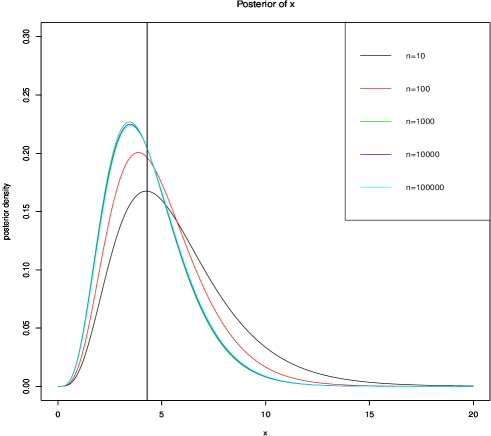
To give an example of inconsistency in non-linear and non-normal inverse problem, consider the following set-up: , for , where and for each . Let us consider the prior for all . For some let us assume the leave-one-out cross-validation set-up in that we wish to learn assuming it is unknown, from the rest of the data. Putting the prior for , the posterior of is given by (see Bhattacharya and Haslett [10], Bhattacharya [9])
| (7.14) |
Figure 7.1 displays the posterior of when , for increasing sample size. Observe that the variance of the posterior does not decrease even with sample size as large as , clearly demonstrating inconsistency. Hence, special, innovative priors are necessary for consistency in such cases.
8 Conclusion
In this review article, we have clarified the similarities and dissimilarities between the traditional inverse problems and the inverse regression problems. In particular, we have argued that only the latter class of problems qualify as authentic inverse problems in they have significantly different goals compared to the corresponding forward problems. Moreover, they include the traditional inverse problems on learning unknown functions as a special case, as exemplified by our palaeoclimate and Milky Way examples. We advocate the Bayesian paradigm for both classes of problems, not only because of its inherent flexibility, coherency and posterior uncertainty quantification, but also because the prior acts as a natural penalty which is very important to regularize the so-called ill-posed inverse problems. The well-known Tikhonov regularizer is just a special case from this perspective.
It is important to remark that the literature on inverse function learning problems and inverse regression problems is still very young and a lot of research is necessary to develop the fields. Specifically, there is hardly any well-developed, consistent model adequacy test or model comparison methodology in either of the two fields, although Mohammad-Djafari [25] deal with some specific inverse problems in this context, and Bhattacharya [9] propose a test for model adequacy in the case of inverse regression problems. Moreover, as we have demonstrated, inverse regression problems are inconsistent in general. The general development in these respects will be provided in the PhD thesis of the first author.
References
References
- [1]
- Arbogast and Bona [2008] Arbogast, T., and Bona, J. L. [2008], “Methods of Applied Mathematics,”. University of Texas at Austin.
- Aronszajn [1950] Aronszajn, N. [1950], “Theory of Reproducing Kernels,” Transactions of the American Mathematical Society, 68, 337–404.
- Aster et al. [2013] Aster, R. C., Borchers, B., and Thurber, C. H. [2013], Parameter Estimation and Inverse Problems, Oxford, UK: Academic Press.
- Avenhaus et al. [1980] Avenhaus, R., Höpfinger, E., and Jewell, W. S. [1980], “Approaches to Inverse Linear Regression,”. Technical Report. Available at https://publikationen.bibliothek.kit.edu/270015256/3812158.
- Baker [1977] Baker, C. T. H. [1977], The Numerical Treatment of Integral Equations, Oxford: Clarendon Press.
- Berger [1985] Berger, J. O. [1985], Statistical Decision Theory and Bayesian Analysis, New York: Springer-Verlag.
- Bhattacharya [2006] Bhattacharya, S. [2006], “A Bayesian Semiparametric Model for Organism Based Environmental Reconstruction,” Environmetrics, 17(7), 763–776.
- Bhattacharya [2013] Bhattacharya, S. [2013], “A Fully Bayesian Approach to Assessment of Model Adequacy in Inverse Problems,” Statistical Methodology, 12, 71–83.
- Bhattacharya and Haslett [2007] Bhattacharya, S., and Haslett, J. [2007], “Importance Resampling MCMC for Cross-Validation in Inverse Problems,” Bayesian Analysis, 2, 385–408.
- Bühlmann and van de Geer [2011] Bühlmann, P., and van de Geer, S. [2011], Statistics for High-Dimensional Data, New York: Springer.
- Bui-Thanh [2012] Bui-Thanh, T. [2012], “A Gentle Tutorial on Statistical Inversion Using the Bayesian Paradigm,”. ICES Report 12-18. Available at http://users.ices.utexas.edu/ tanbui/PublishedPapers/BayesianTutorial.pdf.
- Calvetti and Somersalo [2007] Calvetti, D., and Somersalo, E. [2007], Introduction to Bayesian Scientific Computing: Ten Lectures on Subjective Computing, New York: Springer.
- Chakrabarty et al. [2015] Chakrabarty, D., Biswas, M., and Bhattacharya, S. [2015], “Bayesian Nonparametric Estimation of Milky Way Parameters Using Matrix-Variate Data, in a New Gaussian Process Based Method,” Electronic Journal of Statistics, 9, 1378–1403.
- Dashti and Stuart [2015] Dashti, M., and Stuart, A. M. [2015], “The Bayesian Approach to Inverse Problems,”. eprint: arXiv:1302.6989.
- Duchon [1977] Duchon, J. [1977], Splines Minimizing Rotation-Invariant Semi-norms in Sobolev Spaces,, in Constructive Theory of Functions of Several Variables, eds. W. Schempp, and K. Zellner, Springer-Verlag, New York, pp. 85–100.
- Engl et al. [1996] Engl, H. W., Hanke, M., and Neubauer, A. [1996], Regularization of Inverse Problems, Dordrecht: Kluwer Academic Publishers Group. Volume 375 of Mathematics and its Applications.
- Giraud [2015] Giraud, C. [2015], Introduction to High-Dimensional Statistics, New York: Chapman and Hall.
- Haslett et al. [2006] Haslett, J., Whiley, M., Bhattacharya, S., Salter-Townshend, M., Wilson, S. P., Allen, J. R. M., Huntley, B., and Mitchell, F. J. G. [2006], “Bayesian Palaeoclimate Reconstruction (with discussion),” Journal of the Royal Statistical Society: Series A (Statistics in Society), 169, 395–438.
- Hoadley [1970] Hoadley, B. [1970], “A Bayesian Look at Inverse Linear Regression,” Journal of the American Statistical Association, 65, 356–369.
- Kimeldorf and Wahba [1971] Kimeldorf, G., and Wahba, G. [1971], “Some Results on Tchebycheffian Spline Functions,” Journal of Mathematical Analysis and Applications, 33, 82–95.
- König [1986] König, H. [1986], Eigenvalue Distribution of Compact Operators, : Birkhäuser.
- Krutchkoff [1967] Krutchkoff, R. G. [1967], “Classical and Inverse Regression Methods of Calibration,” Technometrics, 9, 425–435.
- Meinguet [1979] Meinguet, J. [1979], “Multivariate Interpolation at Arbitrary Points Made Simple,” Journal of the Applied Mathematics and Physics, 30, 292–304.
- Mohammad-Djafari [2000] Mohammad-Djafari, A. [2000], “Model Selection for Inverse Problems: Best Choice of Basis Function and Model Order Selection,”. Available at https://arxiv.org/abs/math-ph/0008026.
- Mukhopadhyay and Bhattacharya [2013] Mukhopadhyay, S., and Bhattacharya, S. [2013], “Cross-Validation Based Assessment of a New Bayesian Palaeoclimate Model,” Environmetrics, 24, 550–568.
- Muth [1960] Muth, R. F. [1960], The Demand for Non-Farm Housing,, in The Demand for Durable Goods, ed. A. C. Harberger. The University of Chicago.
- O’Sullivan [1986] O’Sullivan, F. [1986], “A Statistical Perspective on Ill-Posed Inverse Problems,” Statistical Science, 1, 502–512.
- O’Sullivan et al. [1986] O’Sullivan, F., Yandell, B. S., and Raynor, W. J. [1986], “Automatic Smoothing of Regression Functions in Generalized Linear Models,” Journal of the American Statistical Association, 81, 96–103.
- Press and Scott [1975] Press, S. J., and Scott, A. [1975], Missing Variables in Bayesian Regression,, in Studies in Bayesian Econometrics and Statistics, eds. S. E. Fienberg, and A. Zellner, North-Holland, Amsterdam.
- Rasch et al. [1973] Rasch, D., Enderlein, G., and Herrendörfer, G. [1973], “Biometrie,”. Deutscher Landwirtschaftsverlag, Berlin.
- Rasmussen and Williams [2006] Rasmussen, C. E., and Williams, C. K. I. [2006], Gaussian Processes for Machine Learning, Cambridge, Massachusetts: The MIT Press.
- Schölkopf and Smola [2002] Schölkopf, B., and Smola, A. J. [2002], Learning with Kernels, USA: MIT Press.
- Shepp [1966] Shepp, L. A. [1966], “Radon-Nikodym Derivatives of Gaussian Measures,” Annals of Mathematical Statistics, 37, 321–354.
- Tikhonov [1963] Tikhonov, A. [1963], “Solution of Incorrectly Formulated Problems and the Reguarization Method,” Soviet Math. Dokl., 5, 1035–1038.
- Tikhonov and Arsenin [1977] Tikhonov, A., and Arsenin, V. [1977], Solution of Ill-Posed Problems, New York: Wiley.
- Vollmer [2013] Vollmer, S. [2013], “Posterior Consistency for Bayesian Inverse Problems Through Stability and Regression Results,” Inverse Problems, 29. Article number 125011.
- Wahba [1978] Wahba, G. [1978], “Improper Priors, Spline Smoothing and the Problem of Guarding Against Model Errors in Regression,” Journal of the Royal Statistical Society B, 40, 364–372.
- Wahba [1990] Wahba, G. [1990], “Spline Functions for Observational Data,”. CBMS-NSF Regional Conference series, SIAM. Philadelphia.
- Williams [1969] Williams, E. J. [1969], “A Note on Regression Methods in Calibration,” Technometrics, 11, 189–192.