Stochastic efficiency of an isothermal work-to-work converter engine

Abstract

We investigate the efficiency of an isothermal Brownian work-to-work converter engine, composed of a Brownian particle coupled to a heat bath at a constant temperature. The system is maintained out of equilibrium by using two external time-dependent stochastic Gaussian forces, where one is called load force and the other is called drive force. Work done by these two forces are stochastic quantities. The efficiency of this small engine is defined as the ratio of stochastic work done against load force to stochastic work done by the drive force. The probability density function as well as large deviation function of the stochastic efficiency are studied analytically and verified by numerical simulations.

I Introduction

Heat engine Callen (1985); Zemansky (1968) is a machine that operates between two temperatures in a cyclic process. It converts a part of the heat $Q_{H}$ taken from the hot reservoir at a temperature $T_{H}$ to useful work $W,$ and the remaining part of the heat $Q_{C}$ is dumped into the cold reservoir at a temperature $T_{C}<T_{H}$. At the end of the cyclic process, the engine returns to its initial state. The efficiency of an engine is given by the ratio of work done by it to the heat consumed from the hot reservoir: $\eta=W/Q_{H}$. When such engines work in the quasi-static limit as well as in a reversible fashion, its efficiency is given by the Carnot efficiency $\eta_{C}=1-T_{C}/T_{H}$. The efficiency of any engine is bounded above by the Carnot efficiency: $\eta\leq\eta_{C}$. This bound is universal, and does not depend upon the nature of the composition of the engine. In the quasi-static regime, the power delivered by the engine is identically zero: $W/t\ \to 0$ in the limit $t\to\infty$. Therefore, the Carnot engine is not useful for doing work in a reasonable time in practice.

Modern technology helps in engineering machines on a microscopic scale. These small nanosized devices can be seen in many areas of biological science Alberts et al. (2014); Sugawa et al. (2016); Lau et al. (2007); Gelles and Landick (1998); Kinosita et al. (2000); Bustamante et al. (2001). The fluctuations present in the surrounding environment can disturb the deterministic nature of such small-scale devices. Nevertheless, the state of the system can be described in the probabilistic manner, whose evolution is governed by the master equation or Fokker-Planck equation. Interestingly, nowadays various properties of these small systems can be understood by realizing them in controlled experiments Blickle and Bechinger (2012); Martinez et al. (2016); Krishnamurthy et al. (2016); Saira et al. (2012); Toyabe et al. (2010); Ciliberto et al. (2013); Collin et al. (2005); Ciliberto et al. (2010); Gomez-Solano et al. (2011).

When such small-scale machines are driven by external forces, like temperature or concentration gradient, shear flow, time-dependent external field, etc., observables such as work done, heat flow, power injection, entropy production, etc., become stochastic quantities Sabhapandit (2012, 2011); Pal and Sabhapandit (2013, 2014); Verley et al. (2014a); van Zon and Cohen (2003a, b, 2004); Wang et al. (2002); Visco (2006); Kundu et al. (2011); Farago (2002); Gupta and Sabhapandit (2016). The probability distributions of these quantities have richer information than their ensemble average values.

Over the past two decades, a lot of research has been devoted to refining the thermodynamic principle in the mesoscopic scale. While the first law of thermodynamics is also valid at the trajectory level, the second law of thermodynamics is replaced by the symmetry property of the probability distribution of total entropy production Sekimoto (1997); Seifert (2005, 2008). This symmetry property is referred to as the fluctuation theorem (FT) Evans et al. (1993); Evans and Searles (1994); Searles and Evans (2000, 2001); Gallavotti and Cohen (1995); Kurchan (1998); Lebowitz and Spohn (1999); Crooks (1998, 1999, 2000), which accounts for the measure of the likelihood of trajectories violating the second law of thermodynamics.

For a small-scale heat engine connected to two heat reservoirs, the efficiency becomes a fluctuating quantity, whose value changes from one measurement to the other. Hence, it is described by a probability distribution $P(\eta,t)$. In particular, one is interested in its large deviation form Touchette (2009) $P(\eta,t)\sim e^{tJ(\eta)}$, where $J(\eta)$ is the large deviation function defined as $J(\eta)=\lim_{t\to\infty}\frac{1}{t}\ln P(\eta)$. It captures the large time statistics of the efficiency of the stochastic engine. In a recent study, Verley et al. Verley et al. (2014b) computed the large deviation function $J(\eta)$ using FT for microscopic heat engine using two set of examples: work to work converter engine and a photoelectric device. They have shown that the Carnot efficiency is least likely in the long time limit, which is a remarkable result. Moreover, the large deviation function has two extrema: a maximum corresponds to the most probable efficiency, and the minimum occurs at Carnot efficiency. In a similar context, Verley et al. Verley et al. (2014c), found an efficient way to compute the large deviation function of stochastic efficiency using the cumulant generating function of entropy productions for a small engine with finite state space. This method was verified by considering an example of a stochastic engine made up of a system of two states where each of these states is coupled to a heat reservoir at a distinct temperature. To drive this system in the nonequilibrium state, a time-dependent periodic field is applied. They have computed the large deviation function for stochastic efficiency which supported the prediction given in Ref. Verley et al. (2014b). Gingrich et al. Gingrich et al. (2014) computed the finite time probability density function for stochastic efficiency of a two-level heat engine using time-asymmetric driving in a cyclic process. Polettini et al. Polettini et al. (2015) derived the probability density function for stochastic efficiency where thermodynamic fluxes are distributed by a multivariate Gaussian distribution. Using FT for entropy production, it is shown that the probability of efficiency larger than the Carnot one, called super-Carnot efficiency, is favored by trajectories violating the second law of thermodynamics. Moreover, the distribution function has two maxima and one minimum: one maximum corresponds to the most probable efficiency, while the other is at efficiency larger than the Carnot efficiency. The location of the minimum is at the Carnot efficiency. It is observed that the other maximum does not appear in the large deviation function because in the long time limit that maximum occurs at infinity. Proesmans et al. Proesmans et al. (2015) considered an effusion process using two compartments at different temperatures and chemical potentials, where particles flow from a compartment at a higher temperature and low chemical potential to the compartment at a low temperature and high chemical potential. In the finite and long time limit, the distribution for the stochastic efficiency is computed for this effusion engine. Some of these models are briefly discussed in Ref. Proesmans and den Broeck (2015). In the case of isothermal energy transformation Proesmans et al. (2016a), authors considered a Brownian particle in a harmonic potential driven by a duo of time-periodic forces. This setup is used as an engine which converted the Gaussian stochastic input work to Gaussian stochastic output work. They have reproduced the latest discovered connection between different operational regimes (maximum power, maximum efficiency, minimum dissipation) Benenti et al. (2011); Shiraishi et al. (2016); Proesmans et al. (2016b). Moreover, the probability density function for stochastic efficiency is also computed, and all of these results were verified experimentally by them. Park et al. Park et al. (2016) modeled an engine which is driven by time-independent (time-symmetric) driving. In contrast to Refs. Verley et al. (2014b, c), the phase space is found to be continuous with infinite microstates, and it has been shown that the large deviation function does not follow the universal nature as mentioned in Refs. Verley et al. (2014b, c).

In this paper, we mainly focus on an isothermal energy converter where a system consists of a Brownian particle coupled to a heat bath at a constant temperature. In the absence of external forces, total entropy production is identically zero as the system, described by the velocity variable, enjoys equilibrium. The given system is maintained in nonequilibrium steady state using two time-dependent stochastic Gaussian external forces. This system functions as an engine which converts one form of the work (input work) into another form (output work). Note that this engine is different from the usual heat engines where the working substance undergoes the cyclic transformation between two temperatures. Such an isothermal engine can be seen in biological systems, for example, adenosine triphosphate functions as an energy converter in the cell Alberts et al. (2014); Sugawa et al. (2016). The work done by these forces is stochastic random variables. The efficiency of these isothermal engines is defined by the ratio of the work done against the load force to the work done by the drive force, which is also a stochastic quantity. We compute the distribution of stochastic efficiency from the joint distribution of work done against the load force (output work) and work done by the drive force (input work). There are three important features of this paper: (1) We have applied stochastic forces to drive the system out of equilibrium, (2) FT for the joint probability distribution of input and output work does not remain valid for all strength of stochastic forces, and (3) the phase space is continuous with infinite microstates. While the first two features were not introduced in this context earlier as reported in Refs. Proesmans et al. (2016a); Park et al. (2016), the third feature is similar to as mentioned in Ref. Park et al. (2016).

The remainder of the paper is organized as follows. In Sec. II, we give a model system of an engine which converts the input work to the output work. Section III contains the calculation of the joint characteristic function of the input and output work, $Z(\lambda_{1},\lambda_{2})\sim g(\lambda_{1},\lambda_{2})e^{(t/t_{\gamma})\mu(\lambda_{1},\lambda_{2})}$ at large $t$. In Sec. IV, we discuss the method to invert the characteristic function $Z(\lambda_{1},\lambda_{2})$ to get the probability density function $P_{t}(W_{1},W_{2})$. In Sec. IV.1, we analyze the singularity present in $g(\lambda_{1},\lambda_{2})$. In Sec. IV.2, we write the asymptotic expression for the joint probability density $P_{t}(W_{1},W_{2})$ using a saddle point approximation in the absence of a singularity in the prefector $g(\lambda_{1},\lambda_{2})$, and in Sec. IV.3, we discuss the joint probability density function $P_{t}(W_{1},W_{2})$ in the presence of a singularity in $g(\lambda_{1},\lambda_{2})$. FT for $P_{t}(W_{1},W_{2})$ is discussed in Sec. IV.4. In Sec. V.1, we give the expression for the probability density function for stochastic efficiency $P(\eta,t)$ when $g(\lambda_{1},\lambda_{2})$ does not have singularities, and the result for this case is shown in Sec. V.2. In the case, when $g(\lambda_{1},\lambda_{2})$ has singularities, we discuss the methodology to get the asymptotic expression for $P(\eta,t)$ in Sec. V.3, and results in this case are shown in Secs. V.5 and  V.6. We summarized our paper in Sec. VI. Some of the results are given in the Appendix.

II Isothermal work-to-work converter engine

Consider a Brownian particle of mass $m$ immersed in a heat bath of a constant temperature $T$. In the absence of the external driving to the particle, this system reaches an equilibrium state as given by the Gibbs-Boltzmann measure. To model this Brownian particle as an engine, we apply two different time-dependent forces on it. These forces are called load force and drive force. The function of drive force is to drive Brownian particle against the load force. For simplicity, we assume these forces are uncorrelated. The dynamics of the engine is governed by the Langevin equation,

$$m\dot{v}=-\gamma v+\xi(t)+f_{1}(t)+f_{2}(t),$$ (1)

where $v$ is the velocity of the Brownian particle, $\gamma$ is the dissipation constant, and $\xi(t)$ is the Gaussian white noise from the bath, with mean zero and variance $\langle\xi(t)\xi(t^{\prime})\rangle=2T\gamma\delta(t-t^{\prime})$, according to the fluctuation-dissipation theorem. We set Boltzmann’s constant to unity throughout the calculation. The load force $f_{1}(t)$ and the drive force $f_{2}(t)$ are external stochastic Gaussian forces with mean zero and variances $\langle f_{i}(t)f_{j}(t^{\prime})\rangle=\delta_{i,j}\bar{f}_{i}^{2}\delta(t-t^{\prime})$. They are uncorrelated with the thermal noise $\langle f_{i}(t)\xi(t^{\prime})\rangle=0$ for all $t,t^{\prime}$. It turns out that only the relative strengths amongst the external forces and the thermal noise are important, not their absolute values. Therefore, we set $\bar{f}_{1}^{2}=2T\gamma\theta$ and $\bar{f}_{2}^{2}=2T\gamma\theta\alpha^{2}$, where $\theta$ and $\alpha$ are positive parameters.

Multiplying both sides of Eq. (1) by $v$, and integrating with respect to time from $0$ to $t$, yields the conservation of energy relation (first law of thermodynamics)

$$\Delta E=Q+W_{1}+W_{2},$$ (2)

where

$$\Delta E =\frac{m}{2T}[v^{2}(t)-v^{2}(0)],$$ (3)

$$Q =\dfrac{1}{T}\int_{0}^{t}dt^{\prime}\ [\xi(t^{\prime})-\gamma v(t^{\prime})]v(t^{\prime}),$$ (4)

$$W_{1} =\dfrac{1}{T}\int_{0}^{t}dt^{\prime}\ f_{1}(t^{\prime})v(t^{\prime}),$$ (5)

$$W_{2} =\dfrac{1}{T}\int_{0}^{t}dt^{\prime}\ f_{2}(t^{\prime})v(t^{\prime})..$$ (6)

Here, we measure change in the internal energy $\Delta E$, heat absorbed from the surrounding bath $Q$, and work done by load and drive forces $W_{1}$ and $W_{2}$, respectively, in the scale of temperature of the heat bath. The integrals given in Eqs. (4)–(6) follow the Stratonovich rule of integration.

It is clear from Eq. (1) that the velocity $v$ depends linearly on both thermal noise $\xi(t)$ and external Gaussian forces $f_{1}(t)$ and $f_{2}(t)$. Therefore, the distribution of $v(t)$ is Gaussian, where the mean and the variance can easily be computed from Eq. (1). In the limit $t\to\infty$, the mean velocity becomes zero, and the variance is given by

$$\left[\langle v^{2}(t)\rangle-\langle v(t)\rangle^{2}\right]_{t\to\infty}=\dfrac{T(1+\theta+\theta\alpha^{2})}{m}.$$ (7)

On the other hand, $W_{1}$ and $W_{2}$ given in Eqs. (5) and (6), respectively, depend on thermal noise $\xi(t)$ and external Gaussian forces $f_{1}(t)$ and $f_{2}(t)$ quadratically. Thus, the joint distribution $P_{t}(W_{1},W_{2})$ is not expected to be Gaussian.

The quantity of interest is the the efficiency of a stochastic engine $\eta$ which converts the input work $W_{2}$ to the output work $-W_{1}$:

$$\eta=-\dfrac{W_{1}}{W_{2}}.$$ (8)

The distribution of this stochastic efficiency $P(\eta,t)$ is computed from the joint distribution of input and output work $P_{t}(W_{1},W_{2})$ by integrating over $W_{1}$ while using the Dirac delta function $\delta(\eta+W_{1}/W_{2})$. Therefore,

$$P(\eta,t) =\int_{-\infty}^{\infty}dW_{2}\ |W_{2}|\ P_{t}(-\eta W_{2},W_{2}),$$ (9)

where $|W_{2}|$ is the Jacobian.

Note that, when the joint distribution $P_{t}(W_{1},W_{2})$ is Gaussian (that is not the case here),

$$P_{t}(W_{1}=w_{1}t,W_{2}=w_{2}t)=\dfrac{1}{t\sqrt{(2\pi)^{2}\det{C}}}e^{-\frac{t}{2}\bar{w}^{T}C^{-1}\bar{w}},$$ (10)

using Eq. (9), the distribution of the stochastic efficiency $P(\eta,t)$ can easily be shown to be Verley et al. (2014b)

$$P(\eta,t)=\dfrac{e^{j(\eta)t}}{\sqrt{(2\pi)^{2}\det C}}$$

$$\times\dfrac{[2e^{-\frac{t}{2}a(\eta)b(\eta)^{2}}+b(\eta)\sqrt{2\pi t\ a(\eta)}\operatorname{\mathrm{erf}}\big{(}b(\eta)\sqrt{a(\eta)\ t/2}\big{)}]}{a(\eta)},$$ (11)

where $\bar{w}^{T}=(w_{1}-\mu_{1},w_{2}-\mu_{2})$, $C_{ij}=(\langle W_{i}W_{j}\rangle-\langle W_{i}\rangle\langle W_{j}\rangle)/t$, $\mu_{i}=\langle W_{i}\rangle/t$, and

$$j(\eta) =-\dfrac{1}{2}\dfrac{(\eta\mu_{2}+\mu_{1})^{2}}{C_{22}\eta^{2}+2C_{12}\eta+C_{11}}$$ (12)

$$a(\eta) =\dfrac{(\eta C_{22}+C_{12})^{2}+\det{C}}{C_{22}\det{C}}$$ (13)

$$b(\eta) =\dfrac{(C_{11}+C_{12}\eta)\mu_{2}-(C_{12}+C_{22}\eta)\mu_{1}}{C_{22}\eta^{2}+2C_{12}\eta+C_{11}}.$$ (14)

In Eq. (11), $\operatorname{\mathrm{erf}}(u)$ is the error function given by

$$\operatorname{\mathrm{erf}}(u)=\dfrac{2}{\sqrt{\pi}}\int_{0}^{u}e^{-x^{2}}\ dx.$$ (15)

The goal of this paper is to understand the statistics of the efficiency fluctuation when $P_{t}(W_{1},W_{2})$ is non-Gaussian.

III Fokker-Planck equation

To compute $P_{t}(W_{1},W_{2})$, it is convenient to first compute the characteristic function $Z(\lambda_{1},\lambda_{2})=\langle\exp(-\lambda_{1}W_{1}-\lambda_{2}W_{2})\rangle$. The conditional characteristic function $Z(\lambda_{1},\lambda_{2},v,t|v_{0})$ for fixed initial and final conditions, $v(0)=v_{0}$ and $v(t)=v$, satisfies

$$\dfrac{\partial Z(\lambda_{1},\lambda_{2},v,t|v_{0})}{\partial t}=\mathcal{L}_{\lambda_{1},\lambda_{2}}Z(\lambda_{1},\lambda_{2},v,t|v_{0}),$$ (16)

where the differential operator $\mathcal{L}_{\lambda_{1},\lambda_{2}}$ is given by

$$\mathcal{L}_{\lambda_{1},\lambda_{2}}= \bigg{[}\dfrac{T\gamma(1+\theta+\theta\alpha^{2})}{m^{2}}\dfrac{\partial^{2}}{\partial v^{2}}+\dfrac{\gamma[1+2\theta(\lambda_{1}+\alpha^{2}\lambda_{2})]}{m}v\dfrac{\partial}{\partial v}$$

$$+\bigg{\{}\dfrac{\gamma[1+\theta(\lambda_{1}+\alpha^{2}\lambda_{2})]}{m}+\dfrac{\lambda_{1}^{2}+\alpha^{2}\lambda_{2}^{2}}{T}\gamma\theta v^{2}\bigg{\}}\bigg{]}.$$ (17)

The differential equation given in Eq. (16) is subject to initial condition $Z(\lambda_{1},\lambda_{2},v,0|v_{0})=\delta(v-v_{0})$. Note that, putting $\lambda_{1}=\lambda_{2}=0$ in $Z(\lambda_{1},\lambda_{2},v,t|v_{0})$, gives the distribution of velocity $v$ at time $t$ for given initial velocity $v_{0}$, $P(v,t|v_{0})=Z(0,0,v,t|v_{0})$. Consequently, the steady-state velocity distribution is given by $P_{ss}(v)=Z(0,0,v,t\to\infty|v_{0})$, independent of $v_{0}$.

The characteristic function $Z(\lambda_{1},\lambda_{2})$ is obtained from $Z(\lambda_{1},\lambda_{2},v,t|v_{0})$ by averaging over the initial velocity with respect to the steady-state distribution $P_{ss}(v_{0})$ and integrating over the final velocity $v$:

$$Z(\lambda_{1},\lambda_{2})=\int_{-\infty}^{+\infty}dv\ \int_{-\infty}^{+\infty}dv_{0}\ P_{ss}(v_{0})\ Z(\lambda_{1},\lambda_{2},v,t|v_{0}).$$ (18)

To solve differential equation given in Eq. (16), we write

$$Z(\lambda_{1},\lambda_{2},v,t|v_{0})=e^{-\frac{1}{2T}[U(v)-U(v_{0})]}\ \psi_{\lambda_{1},\lambda_{2}}(v,t|v_{0}).$$ (19)

It follows that, for the particular choice

$$U(v)=\dfrac{m[1+2\theta(\lambda_{1}+\alpha^{2}\lambda_{2})]}{2(1+\theta+\theta\alpha^{2})}v^{2},$$ (20)

$\Psi_{\lambda_{1},\lambda_{2}}(v,t|v_{0})$ satisfies the Schrödinger equation in the imaginary time $-i\hbar t$ (and identifying $[T\gamma(1+\theta+\theta\alpha^{2})/m^{2}]$ with $[\hbar^{2}/(2m_{q})]$ in the quantum problem),

$$\dfrac{\partial\psi_{\lambda_{1},\lambda_{2}}(v,t|v_{0})}{\partial t}=\bigg{[}\dfrac{T\gamma(1+\theta+\theta\alpha^{2})}{m^{2}}\dfrac{\partial^{2}}{\partial v^{2}}-V(v)\bigg{]}\psi_{\lambda_{1},\lambda_{2}}(v,t|v_{0}),$$

for a quantum harmonic oscillator (QHO), where

$$V(v)=\frac{1}{2}m_{q}w_{q}^{2}v^{2}-\dfrac{\gamma}{2m},$$ (22)

with the identification

$$m_{q}w_{q}^{2}=\dfrac{\gamma}{T}\bigg{[}\dfrac{[1+2\theta(\lambda_{1}+\alpha^{2}\lambda_{2})]^{2}}{2(1+\theta+\theta\alpha^{2})}-2\theta(\lambda_{1}^{2}+\alpha^{2}\lambda_{2}^{2})\bigg{]}.$$ (23)

Thus, $\psi_{\lambda_{1},\lambda_{2}}(v,t|v_{0})=\langle v|e^{-\hat{H}t}|v_{0}\rangle$ is recognized as the propagator of the QHO, which is known exactly. For our purpose, it is convenient to expand $\psi_{\lambda_{1},\lambda_{2}}(v,t|v_{0})$ in the eigenbasis $\{\psi_{n}(v)\}$ of $\hat{H}$ as

$$\psi_{\lambda_{1},\lambda_{2}}(v,t|v_{0})=\sum_{n=0}^{\infty}e^{-tE_{n}(\lambda_{1},\lambda_{2})}\psi_{n}(v)\psi_{n}^{*}(v_{0}),$$ (24)

where the eigenvalues are given by

$$E_{n}=\left(n+\frac{1}{2}\right)\hbar w_{q}-\dfrac{\gamma}{2m},\quad n=0,1,2,\dotsc.$$ (25)

From the above identification between the quantum and the stochastic problem, we have

$$\hbar w_{q}=(\gamma/m)\nu(\lambda_{1},\lambda_{2})$$ (26)

with

$$\nu(\lambda_{1},\lambda_{2})=\big{[}1+4\theta\{\lambda_{1}(1-\lambda_{1})+\alpha^{2}\lambda_{2}(1-\lambda_{2})$$

$$-\alpha^{2}\theta(\lambda_{1}-\lambda_{2})^{2}\}\big{]}^{1/2}.$$ (27)

In the long time limit, Eq. (24) is dominated by the $n=0$ (ground state) term. Thus, for large $t$, Eq. (19) becomes

$$Z(\lambda_{1},\lambda_{2},v,t|v_{0})=e^{(t/t_{\gamma})\ \mu(\lambda_{1},\lambda_{2})}\Psi(v,\lambda_{1},\lambda_{2})\chi(v_{0},\lambda_{1},\lambda_{2})+\dotsb$$ (28)

where $t_{\gamma}=m/\gamma$ is the viscous relaxation time, and

$$\mu(\lambda_{1},\lambda_{2}) =\frac{1}{2}[1-\nu(\lambda_{1},\lambda_{2})],$$ (29)

$$\Psi(v,\lambda_{1},\lambda_{2}) =A_{0}\,e^{-\frac{\beta}{2}U(v)}\psi_{0}(v),$$ (30)

$$\chi(v_{0},\lambda_{1},\lambda_{2}) =A_{0}^{-1}\,e^{\frac{\beta}{2}U(v_{0})}\psi_{0}^{*}(v_{0}),$$ (31)

where $A_{0}$ is an arbitrary function of $\lambda_{1}$ and $\lambda_{2}$. Note that $\chi(v_{0},\lambda_{1},\lambda_{2})$ and $\Psi(v,\lambda_{1},\lambda_{2})$, respectively are also the left and right eigenfunctions of the differential operator $\mathcal{L}_{\lambda_{1},\lambda_{2}}$ corresponding to the largest eigenvalue $\mu(\lambda_{1},\lambda_{2})$. Using the ground state eigenfunction of the QHO, with a particular choice of $A_{0}$, it can easily be found that

$$\Psi(v,\lambda_{1},\lambda_{2}) =\sqrt{\dfrac{m\gamma\ \nu(\lambda_{1},\lambda_{2})}{2\pi\ \Theta}}$$

$$\times\exp\bigg{(}-\frac{m\gamma}{4\Theta}[\nu(\lambda_{1},\lambda_{2})+1+2\theta(\lambda_{1}+\alpha^{2}\lambda_{2})]v^{2}\bigg{)},$$ (32)

$$\chi(v_{0},\lambda_{1},\lambda_{2}) =\exp\bigg{(}-\frac{m\gamma}{4\Theta}[\nu(\lambda_{1},\lambda_{2})-1-2\theta(\lambda_{1}+\alpha^{2}\lambda_{2})]v_{0}^{2}\bigg{)},$$ (33)

with $\Theta=T\gamma(1+\theta+\theta\alpha^{2})$. The left and right eigenfunctions satisfy the normalization condition

$$\int_{-\infty}^{+\infty}\chi(v,\lambda_{1},\lambda_{2})\Psi(v,\lambda_{1},\lambda_{2})\ dv=1.$$ (34)

From the above expressions, we find that $\mu(0,0)=0$ and $\chi(v_{0},0,0)=1$. Therefore, the steady state distribution $P_{ss}(v)=Z(0,0,v,t\to\infty|v_{0})$ of the velocity is given by

$$P_{ss}(v)=\Psi(v,0,0)=\sqrt{\dfrac{m\gamma}{2\pi\Theta}}\exp\bigg{[}-\dfrac{m\gamma v^{2}}{2\Theta}\bigg{]}.$$ (35)

The characteristic function $Z(\lambda_{1},\lambda_{2})$ is obtained after carrying out integrals given in Eq. (18),

$$Z(\lambda_{1},\lambda_{2})=g(\lambda_{1},\lambda_{2})\exp[(t/t_{\gamma})\mu(\lambda_{1},\lambda_{2})]+\dotsb.$$ (36)

Here, the prefactor

$$g(\lambda_{1},\lambda_{2})=\dfrac{2\sqrt{\nu(\lambda_{1},\lambda_{2})}}{\sqrt{f^{+}(\lambda_{1},\lambda_{2})}\sqrt{f^{-}(\lambda_{1},\lambda_{2})}},$$ (37)

in which $f^{\pm}(\lambda_{1},\lambda_{2})=1\pm 2\theta(\lambda_{1}+\alpha^{2}\lambda_{2})+\nu(\lambda_{1},\lambda_{2})$. The first factor in the denominator of $g(\lambda_{1},\lambda_{2})$ is due to the integration over the final velocity $v$, and the second factor in the denominator of $g(\lambda_{1},\lambda_{2})$ comes from averaging over the initial velocity $v_{0}$ with respect to steady-state distribution $P_{ss}(v_{0})$.

Note from Eqs. (29) and (37) that largest eigenvalue $\mu(\lambda_{1},\lambda_{2})$ satisfies the Gallavotti-Cohen symmetry whereas the prefactor $g(\lambda_{1},\lambda_{2})$ does not, i.e., $\mu(\lambda_{1},\lambda_{2})=\mu(1-\lambda_{1},1-\lambda_{2})$ and $g(\lambda_{1},\lambda_{2})\neq g(1-\lambda_{1},1-\lambda_{2})$.

IV Joint Probability density function $P_{t}(W_{1},W_{2})$

The joint distribution of input and output work $P_{t}(W_{1},W_{2})$ can be obtained by inverting the characteristic function $Z(\lambda_{1},\lambda_{2})$ given in Eq. (36):

$$P_{t}(W_{1},W_{2})=\int_{-i\infty}^{i\infty}\dfrac{d\lambda_{1}}{2\pi i}\int_{-i\infty}^{i\infty}\dfrac{d\lambda_{2}}{2\pi i}\ Z(\lambda_{1},\lambda_{2})\ e^{\lambda_{1}W_{1}+\lambda_{2}W_{2}}.$$ (38)

Thus, for large $t$,

$$P_{t}(W_{1},W_{2}) =\int_{-i\infty}^{i\infty}\dfrac{d\lambda_{1}}{2\pi i}\int_{-i\infty}^{i\infty}\dfrac{d\lambda_{2}}{2\pi i}\ g(\lambda_{1},\lambda_{2})\ e^{(t/t_{\gamma})\ I_{w_{1},w_{2}}(\lambda_{1},\lambda_{2})}$$

$$+\dotsb,$$ (39)

where $w_{1}=W_{1}t_{\gamma}/t$ and $w_{2}=W_{2}t_{\gamma}/t$ are scaled variables. Here, the contours of integration are taken along $\mathrm{Im}(\lambda_{1})$ and $\mathrm{Im}(\lambda_{2})$ axes passing through the origin of the complex $(\lambda_{1},\lambda_{2})$ plane. The function $I_{w_{1},w_{2}}(\lambda_{1},\lambda_{2})$ is given as

$$I_{w_{1},w_{2}}(\lambda_{1},\lambda_{2})=\mu(\lambda_{1},\lambda_{2})+\lambda_{1}w_{1}+\lambda_{2}w_{2}.$$ (40)

It can be seen $\nu(\lambda_{1},\lambda_{2})$ is a real and positive quantity when $(\lambda_{1},\lambda_{2})\in\mathbb{R}_{1}$ where $\mathbb{R}_{1}$ is the region shown in Fig. 1, bounded by $(\lambda_{1}(\phi),\lambda_{2}(\phi))$ in which

$$\lambda_{1}(\phi)=\dfrac{1}{2}\bigg{[}1+\sqrt{\dfrac{\alpha^{2}\theta}{1+\alpha^{2}\theta}}\sin\phi+\sqrt{\dfrac{1+\theta+\theta\alpha^{2}}{\theta(1+\alpha^{2}\theta)}}\cos\phi\bigg{]},$$ (41)

$$\lambda_{2}(\phi)=\dfrac{1}{2}\bigg{[}1+\sqrt{\dfrac{1+\alpha^{2}\theta}{\alpha^{2}\theta}}\sin\phi\bigg{]},\quad\text{with}\quad\phi\in[-\pi,\pi].$$

Here, $(\lambda_{1}(\phi)$, $\lambda_{2}(\phi))$ is the parametric representation of equation of ellipse [see Eq. (27)]

$$1+4\theta[\lambda_{1}(1-\lambda_{1})+\alpha^{2}\lambda_{2}(1-\lambda_{2})-\alpha^{2}\theta(\lambda_{1}-\lambda_{2})^{2}]=0.$$ (43)

The maximum and minimum values of $\lambda_{1}(\phi)$ and $\lambda_{2}(\phi)$ (see black dashed lines in Fig. 1) are

$$\lambda_{10}^{\pm} =\dfrac{1}{2}\bigg{[}1\pm\sqrt{1+\dfrac{1}{\theta}}\bigg{]},$$ (44)

$$\lambda_{20}^{\pm} =\dfrac{1}{2}\bigg{[}1\pm\sqrt{1+\dfrac{1}{\alpha^{2}\theta}}\bigg{]},$$ (45)

where $+$ and $-$ signs correspond to maximum and minimum value, respectively. Consequently, $I_{w_{1},w_{2}}(\lambda_{1},\lambda_{2})$ is also a real quantity when $(\lambda_{1},\lambda_{2})\in\mathbb{R}_{1}$.

The long-time result of the integral given in Eq. (39) can be approximated using the saddle-point method. The saddle point ($\lambda_{1}^{*},\lambda_{2}^{*}$) can be obtained by solving the following equations simultaneously:

$$\dfrac{\partial I_{w_{1},w_{2}}(\lambda_{1},\lambda_{2})}{\partial\lambda_{1}}\bigg{|}_{\lambda_{1,2}=\lambda_{1,2}^{*}} =0,$$ (46)

$$\dfrac{\partial I_{w_{1},w_{2}}(\lambda_{1},\lambda_{2})}{\partial\lambda_{2}}\bigg{|}_{\lambda_{1,2}=\lambda_{1,2}^{*}} =0.$$ (47)

This gives

$$\lambda_{1}^{*}(w_{1},w_{2}) =\dfrac{1}{2}\bigg{[}1-\dfrac{\alpha[w_{1}+(w_{1}+w_{2})\theta]}{\Lambda}\bigg{]},$$ (48)

$$\lambda_{2}^{*}(w_{1},w_{2}) =\dfrac{-w_{2}-(w_{1}+w_{2})\alpha^{2}\theta+\alpha\Lambda}{2\alpha\Lambda},$$ (49)

where
$\Lambda=\sqrt{\theta[w_{1}^{2}\alpha^{2}+w_{2}^{2}+(w_{1}+w_{2})^{2}\alpha^{2}\theta+\alpha^{2}\theta(1+\theta+\theta\alpha^{2})]}$. Clearly, one can see that $(\lambda_{1}^{*},\lambda_{2}^{*})\in\mathbb{R}_{1}$. Moreover, at the saddle point, the function $I(w_{1},w_{2}):=I_{w_{1},w_{2}}(\lambda_{1}^{*},\lambda_{2}^{*})$ reads as

$$I(w_{1},w_{2})=\dfrac{1}{2}\bigg{[}1+w_{1}+w_{2}-\dfrac{\Lambda}{\alpha\theta}\bigg{]}.$$ (50)

Now, to solve the integral given in Eq. (39), we have to analyze whether $g(\lambda_{1},\lambda_{2})$ is analytic when $(\lambda_{1},\lambda_{2})\in\mathbb{R}_{1}$. If there is no singularity present in $g(\lambda_{1},\lambda_{2})$ between the origin of the $(\lambda_{1},\lambda_{2})$ plane and saddle point ($\lambda_{1}^{*},\lambda_{2}^{*}$), one can deform the contours of integration through the saddle point ($\lambda_{1}^{*},\lambda_{2}^{*}$) and carry out saddle-point integration to approximate the integral given in Eq. (39) Pal and Sabhapandit (2013, 2014); Touchette (2009). However, if $g(\lambda_{1},\lambda_{2})$ contains a singularity between the saddle point and the origin of $(\lambda_{1},\lambda_{2})$ plane, then the saddle-point approximation will not be valid. In the following subsections, we consider both cases.

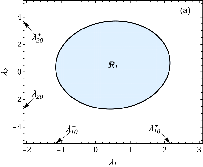
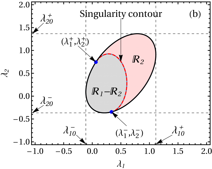
Figure 1: Two scenarios are shown here. (a) $g(\lambda_{1},\lambda_{2})$ is analytic for all $(\lambda_{1},\lambda_{2})\in\mathbb{R}_{1}$. (b) The light red region $\mathbb{R}_{2}$ represents the area where $g(\lambda_{1},\lambda_{2})$ is imaginary, whereas it is real in $\mathbb{R}_{1}-\mathbb{R}_{2}$. The red contour (thick dashed) is the singularity line and corresponds to Eq. (51). End points $(\lambda_{1,2}^{\pm})$ are given in the Appendix. In both cases, the black solid contour represents the region $\mathbb{R}_{1}$ bounded by $(\lambda_{1}(\phi),\lambda_{2}(\phi))$, $\phi\in[-\pi,\pi]$. Black dashed lines show the maximum and minimum values of $\lambda_{1}(\phi)$ and $\lambda_{2}(\phi)$ as given by Eqs. (44) and (45).

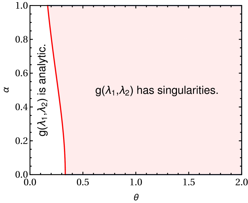
Figure 2: Contour (red solid line) separates two regions depending upon if $g(\lambda_{1},\lambda_{2})$ has singularities or not.

IV.1 Analytic behavior of the correction term $g(\lambda_{1},\lambda_{2})$

In $g(\lambda_{1},\lambda_{2})$, $f^{+}(\lambda_{1},\lambda_{2})>0$ for all $\theta\in(0,\infty)$ and $\alpha\in(0,\infty)$ whereas the function $f^{-}(\lambda_{1},\lambda_{2})$ can attain any sign depending on the values of $\theta$ and $\alpha$. It turns out that there can be two scenarios, which are shown in Fig. 1. In both scenarios, $\mathbb{R}_{1}$ is the region bounded by contour $(\lambda_{1}(\phi),\lambda_{2}(\phi))$ where $\phi\in[-\pi,\pi]$ (see black solid contour in Fig. 1). In Fig. 1(a), $f^{-}(\lambda_{1},\lambda_{2})>0$ for all $(\lambda_{1},\lambda_{2})\in\mathbb{R}_{1}$, and hence $g(\lambda_{1},\lambda_{2})$ does not have any singularity in the whole region $\mathbb{R}_{1}$. On the other hand, in Fig. 1(b), $f^{-}(\lambda_{1},\lambda_{2})\leq 0$ in the region $(\lambda_{1},\lambda_{2})\in\mathbb{R}_{2}$ and positive in $(\lambda_{1},\lambda_{2})\in\mathbb{R}_{1}-\mathbb{R}_{2}$. Hence $g(\lambda_{1},\lambda_{2})$ has singularities given by the curve

$$f^{-}(\lambda_{1},\lambda_{2})=0.$$ (51)

We see two regions in the phase diagram in $(\alpha,\theta)$ plane shown in Fig. 2, which distinguish these two scenarios, and the equation of contour which separates these two regions is given by (see the Appendix)

$$(1+\alpha^{2})\theta=1/3.$$ (52)

In the next subsections, we will discuss both cases one by one.

IV.2 Case 1: Singularity contour is absent

When there is no singularity contour present in the domain $\mathbb{R}_{1}$ [see Fig. 1(a)], we can approximate the integral given in Eq. (39) by the saddle-point method. Therefore, we get

$$P_{t}(W_{1},W_{2})\approx\dfrac{\tilde{g}(w_{1},w_{2})\ e^{(t/t_{\gamma})\ I(w_{1},w_{2})}}{2\pi\ t/t_{\gamma}\sqrt{|\tilde{H}(w_{1},w_{2})|}},$$ (53)

where $\tilde{g}(w_{1},w_{2}):=g(\lambda_{1}^{*},\lambda_{2}^{*})$, and $\tilde{H}(w_{1},w_{2}):=H(\lambda_{1}^{*},\lambda_{2}^{*})$ is the determinant of the Hessian matrix,

$$H(\lambda_{1}^{*},\lambda_{2}^{*}) =\bigg{[}\dfrac{\partial^{2}I(\lambda_{1},\lambda_{2})}{\partial\lambda_{1}^{2}}\dfrac{\partial^{2}I(\lambda_{1},\lambda_{2})}{\partial\lambda_{2}^{2}}$$

$$\quad\quad\quad\quad\quad\quad-\bigg{(}\dfrac{\partial^{2}I(\lambda_{1},\lambda_{2})}{\partial\lambda_{1}\partial\lambda_{2}}\bigg{)}^{2}\bigg{]}\bigg{|}_{\lambda_{1,2}=\lambda_{1,2}^{*}}$$

$$=\dfrac{4\Lambda^{4}}{\alpha^{2}\theta^{2}(1+\theta+\theta\alpha^{2})^{2}}.$$ (54)

The function $I(w_{1},w_{2})$ is given by Eq. (50). Here, $\tilde{H}(w_{1},w_{2})>0$ for all $\theta,\ \alpha,\ w_{1}$, and $w_{2}$ which implies that along axes $\mathrm{Re}(\lambda_{1})$ and $\mathrm{Re}(\lambda_{2})$, function $I_{w_{1},w_{2}}(\lambda_{1},\lambda_{2})$ given in Eq. (40), is minimum at the saddle point $(\lambda_{1}^{*},\lambda_{2}^{*})$ . Therefore, contours of integration are taken along the direction perpendicular to both $\mathrm{Re}(\lambda_{1})$ and $\mathrm{Re}(\lambda_{2})$ axes of the complex $(\lambda_{1},\lambda_{2})$ plane Pal and Sabhapandit (2013, 2014).

IV.3 Case 2: Singularity contour is present

When a singularity contour is present in the region $(\lambda_{1},\lambda_{2})\in\mathbb{R}_{1}$ [see red contour (thick dashed) in Fig. 1(b)], we have to compute the integral given in Eq. (39) carefully. In such a case, there will be two types of contributions, namely, saddle and branch point contributions. When the saddle point $(\lambda_{1}^{*},\lambda_{2}^{*})$ does not cross the branch point contour given by Eq. (51) [see red contour (thick dashed) in Fig. 1(b)] i.e., the saddle point does not enter the light red region $\mathbb{R}_{2}$ of Fig. 1(b), the contribution is the same as given in Eq. (53). As the saddle point crosses the branch point contour given by Eq. (51), then, the integral can not approximated with the usual saddle-point solution, and one has to evaluate Eq. (39) carefully by taking into account of the singularities Pal and Sabhapandit (2013, 2014); Lee et al. (2013); Noh (2014).

Since the equation of the singularity contour is given by Eq. (51), in the $(w_{1},w_{2})$ plane, the contour separating these two regions (saddle and branch points) becomes $h(w_{1},w_{2}):=f^{-}(\lambda_{1}^{*},\lambda_{2}^{*})=0$. The joint probability distribution of $W_{1}$ and $W_{2}$ is given as

$$P_{t}(W_{1},W_{2})=\begin{cases}P_{S}(W_{1},W_{2},t)\quad\quad\quad\quad h(w_{1},w_{2})\gg 0,\\ P_{B}(W_{1},W_{2},t)\quad\quad\quad\quad h(w_{1},w_{2})\ll 0,\\ \end{cases}$$ (55)

where $P_{S}(W_{1},W_{2},t)$ and $P_{B}(W_{1},W_{2},t)$ are saddle and branch point contributions, respectively. Signs $\ll$ and $\gg$ show that both saddle and branch point contributions are valid away from the singularity contour [see the red contour (thick dashed) in Fig. 1(b)] Pal and Sabhapandit (2013, 2014).

IV.4 Large deviation function and FT for joint distribution $P_{t}(W_{1},W_{2})$

The large deviation function is defined as

$$I(w_{1},w_{2})=\lim_{t/t_{\gamma}\ \to\ \infty}\frac{t_{\gamma}}{t}\ln{P_{t}(W_{1},W_{2})},$$ (56)

and the large deviation form of joint distribution is usually written as

$$P_{t}(W_{1},W_{2})\sim e^{(t/t_{\gamma})I(w_{1},w_{2})}.$$ (57)

For the distribution satisfying FT, it is seen that

$$\lim_{t/t_{\gamma}\ \to\ \infty}\dfrac{t_{\gamma}}{t}\ln{\bigg{[}\dfrac{P(W_{1}=+w_{1}t/t_{\gamma},W_{2}=+w_{2}t/t_{\gamma})}{P(W_{1}=-w_{1}t/t_{\gamma},W_{2}=-w_{2}t/t_{\gamma})}\bigg{]}}=w_{1}+w_{2}.$$ (58)

When the above relation holds, the large deviation function satisfies a symmetry property given as

$$I(w_{1},w_{2})-I(-w_{1},-w_{2})=w_{1}+w_{2}\quad\text{for all}\quad(w_{1},w_{2}).$$ (59)

The phase diagram given in Fig. 2 characterizes regions of analyticity for the prefactor $g(\lambda_{1},\lambda_{2})$. If $g(\lambda_{1},\lambda_{2})$ does not have any singularity in the region $(\lambda_{1},\lambda_{2})\in\mathbb{R}_{1}$, the dominant contribution to the joint distribution $P_{t}(W_{1},W_{2})$ comes from the saddle-point approximation as given by Eq. (53). However, when the saddle point $(\lambda_{1}^{*},\lambda_{2}^{*})$ crosses the branch point contour shown in Fig. 1(b) [see light red region $\mathbb{R}_{2}$ of Fig. 1(b)], the contribution to $P_{t}(W_{1},W_{2})$ comes from both saddle and branch points as given by Eq. (55). Thus, for the region where $g(\lambda_{1},\lambda_{2})$ does not have any singularity (see Fig. 2), the large deviation function $I(w_{1},w_{2})$ is given by Eq. (50) and satisfies the relation given in Eq. (59), and hence, the fluctuation theorem is satisfied. On the other hand, when $g(\lambda_{1},\lambda_{2})$ has singularities, the fluctuation theorem would not be satisfied for large $(w_{1},w_{2})$.

V Probability density function of Stochastic efficiency $P(\eta,t)$

After computing the asymptotic form of $P_{t}(W_{1},W_{2})$, we have to carry out one more integral given in Eq. (9) to get the probability density function of stochastic efficiency. There are two cases, which we will discuss in the next subsections.

V.1 Case 1: $g(\lambda_{1},\lambda_{2})$ does not have singularities

When the asymptotic form of $P_{t}(W_{1},W_{2})$ is given by only the saddle-point contribution [see Eq. (53)], then the integral given in Eq. (9) can also be computed using the saddle-point method. In that case, by solving the saddle-point equation

$$\dfrac{\partial I(-\eta w_{2},w_{2})}{\partial w_{2}}\bigg{|}_{w_{2}=w_{2}^{*}}=0,$$ (60)

we find the saddle point $w_{2}^{*}(\eta)$ as

$$w_{2}^{*}(\eta)=\dfrac{(1-\eta)\alpha^{2}\theta\sqrt{1+\theta+\theta\alpha^{2}}}{\sqrt{(1+\eta^{2}\alpha^{2})[1+\eta^{2}\alpha^{2}+\alpha^{2}\theta(1-\eta)^{2}]}}.$$ (61)

Finally, the probability density function for stochastic efficiency is given by

$$P(\eta,t)\approx\dfrac{t\tilde{g}(-\eta w_{2}^{*},w_{2}^{*})\zeta(\eta,t)}{2\pi t_{\gamma}\sqrt{\tilde{H}(-\eta w_{2}^{*},w_{2}^{*})}}\exp[(t/t_{\gamma})\ I(-\eta w_{2}^{*},w_{2}^{*})],$$ (62)

where

$$\zeta(\eta,t)=\dfrac{e^{-KY^{2}}+\sqrt{\pi K}Y\operatorname{\mathrm{erf}}(\sqrt{K}Y)}{K},$$ (63)

with $Y=w_{2}^{*}(\eta)$, $K=t/(2t_{\gamma})\big{|}\partial^{2}I(-\eta w_{2},w_{2})/\partial w_{2}^{2}\big{|}_{w_{2}^{*}}$, and $\operatorname{\mathrm{erf}}(u)$ is given by Eq. (15).

The large deviation function $J(\eta):=I(-\eta w_{2}^{*},w_{2}^{*})$ is given by

$$J(\eta)=\dfrac{1}{2}\bigg{[}1-\sqrt{\dfrac{(1+\alpha^{2}\eta^{2})(1+\theta+\theta\alpha^{2})}{1+\alpha^{2}[\eta^{2}+(1-\eta)^{2}\theta]}}\bigg{]}$$ (64)

The large deviation function $J(\eta)$ for stochastic efficiency has two extrema. The minimum occurs at $\eta^{*}=1$ while the maximum is at $\bar{\eta}=-\alpha^{-2}$. The efficiency at which the large deviation function is minimum is called an analog of the Carnot efficiency Polettini et al. (2015) as this is essentially the maximum value that the efficiency of a reversible engine can achieve in macroscopic systems. At the efficiency $\bar{\eta}$, $J(\bar{\eta})=J^{\prime}(\eta=\bar{\eta})=0$, which are the properties of a large deviation function.

V.2 Numerical simulation

We compare the analytical form given in Eq. (62) with the numerical simulation. We take parameter $\theta=0.1$ and $\alpha=0.5$ at three different times: $t/t_{\gamma}=20$, $t/t_{\gamma}=50$, and $t/t_{\gamma}=100$. Figure 3 shows a very good agreement with simulation and theoretical prediction.

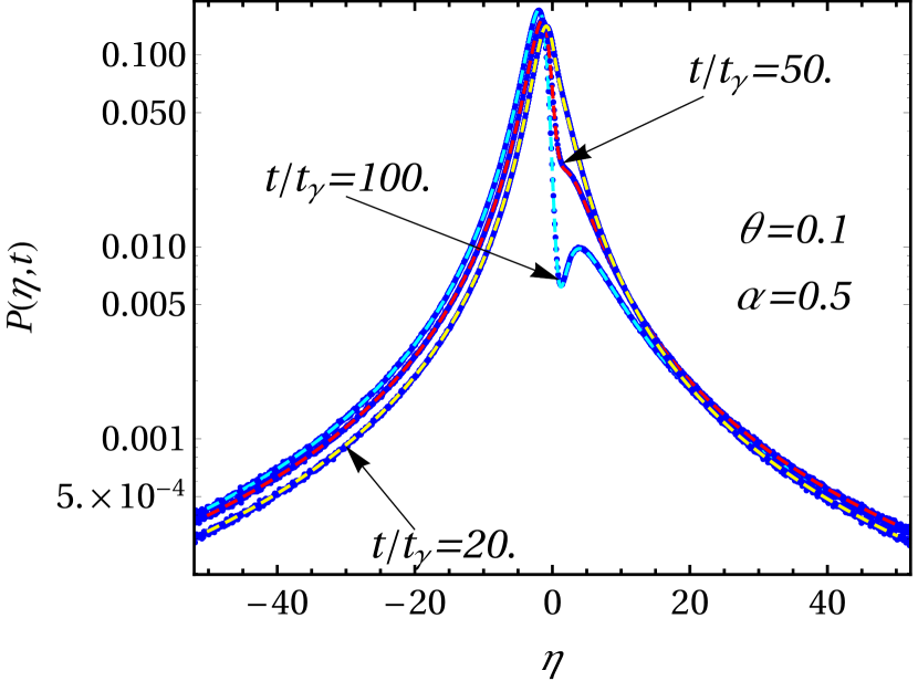
Figure 3: Distribution of stochastic efficiency $P(\eta,t)$ is plotted against the stochastic efficiency $\eta$ for $\theta=0.1$ and $\alpha=0.5$ at three different times: $t/t_{\gamma}=20,50,100$. Yellow $(t/t_{\gamma}=20)$, red $(t/t_{\gamma}=50)$, and cyan $(t/t_{\gamma}=100)$ dashed lines are plotted for analytical expression given in Eq. (62) while the blue dots are for the numerical simulations at the corresponding times $t/t_{\gamma}$.

V.3 Case 2: $g(\lambda_{1},\lambda_{2})$ has singularities

When $g(\lambda_{1},\lambda_{2})$ has singularities in the region $(\lambda_{1},\lambda_{2})\in\mathbb{R}_{1}$ [see Fig. 1(b)], we need to be careful while computing the asymptotic form of $P_{t}(W_{1},W_{2})$, as given by Eq. (55).

It turns out that the saddle point $w_{2}^{*}(\eta)$ given in Eq. (61), from the saddle-point contribution of $P_{t}(-\eta W_{2},W_{2})$ stays either in saddle point region (possibility I) or in both saddle- and branch-point regions (possibility II) of $P_{t}(-\eta w_{2},w_{2})$ depending upon parameters $\theta$ and $\alpha$ as shown in Fig. 4. In Fig. 4 light blue (S.P. region) and light red (B.P. region) regions correspond to the saddle- and branch-point contributions of joint distribution $P_{t}(-\eta W_{2},W_{2})$, respectively.

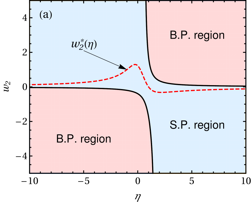
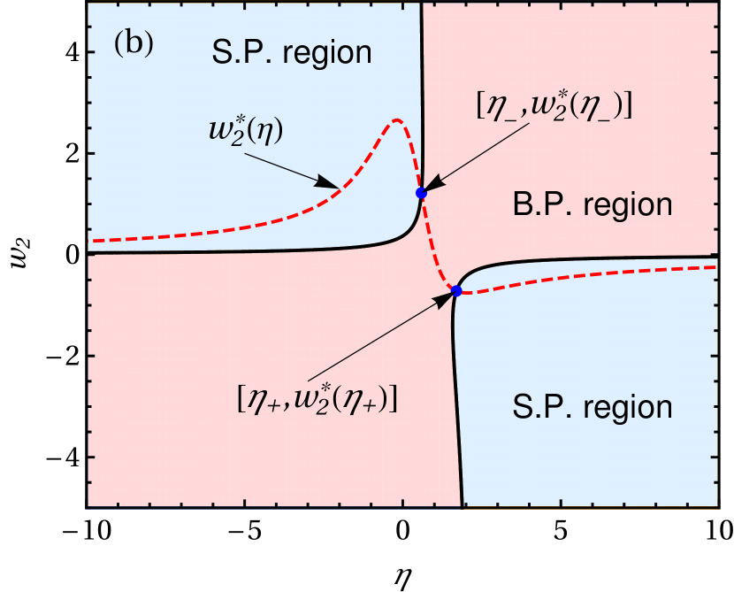
Figure 4: Two possibilities are shown. (a) Saddle point $w_{2}^{*}(\eta)$ stays in the saddle-point region of $P_{t}(-\eta W_{2},W_{2})$. (b) Saddle point $w_{2}^{*}(\eta)$ stays in both the saddle- and branch-point regions of $P_{t}(-\eta W_{2},W_{2})$. Light blue (S.P. region) [$h(-\eta w_{2},w_{2})>0$] and light red (B.P. region) [$h(-\eta w_{2},w_{2})<0$] shaded areas are for saddle- and branch-point contributions of $P_{t}(-\eta W_{2},W_{2})$, respectively. Black solid line corresponds to $h(-\eta w_{2},w_{2})=0$. Blue points are given by $(\eta_{-},w_{2}^{*}(\eta_{-}))$ and $(\eta_{+},w_{2}^{*}(\eta_{+}))$.

As saddle point $w_{2}^{*}(\eta)$ intersects the contour $h(-\eta w_{2},w_{2})=0$, it satisfies

$$h\big{(}-\eta_{\pm}w_{2}^{*}(\eta_{\pm}),w_{2}^{*}(\eta_{\pm})\big{)}=0,$$ (65)

in which

$$\eta_{\pm}=\dfrac{4\alpha\theta\pm\sqrt{3(1+\theta+\theta\alpha^{2})}\sqrt{-3+\theta+\theta\alpha^{2}}}{\alpha[3(1+\theta)-\alpha^{2}\theta]}.$$ (66)

Therefore, points where saddle point $w^{*}(\eta)$ intersects the contour $h(-\eta w_{2},w_{2})=0$ are given by $(\eta_{-},w_{2}^{*}(\eta_{-}))$ and $(\eta_{+},w_{2}^{*}(\eta_{+}))$. The contour, which separates possibility I from possibility II in the $(\theta,\alpha)$ space, is given by the condition $\eta_{+}=\eta_{-}$, which results in

$$-3+\theta+\theta\alpha^{2}=0.$$ (67)

It also follows from the fact that the efficiency is a real quantity, and therefore, $\eta_{\pm}$ must be real, which implies $(-3+\theta+\theta\alpha^{2})\geq 0$.

Using the above equation, we can draw a phase diagram in the $(\theta,\alpha)$ plane as shown in Fig. 5.

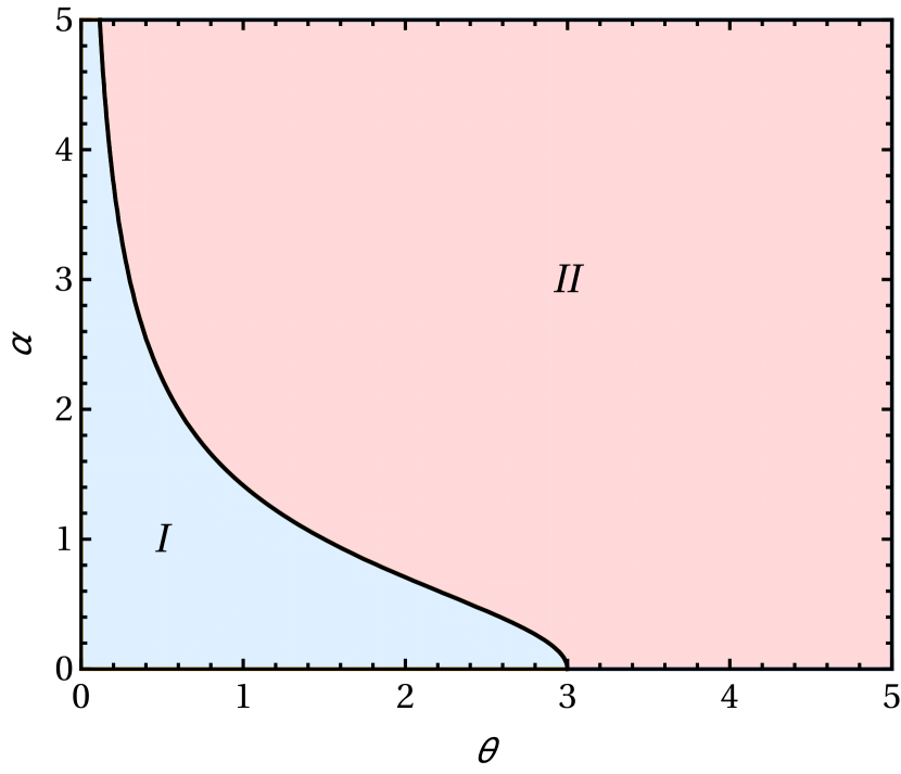
Figure 5: Possibility I: The distribution of efficiency $P(\eta,t)$ can be computed by only saddle point solution given by Eq. (53). Possibility II: The distribution of efficiency $P(\eta,t)$ requires the branch point contribution of $P_{t}(-\eta W_{2},W_{2})$.

In possibility I, saddle point $w^{*}(\eta)$ does not intersect the contour given by $h(-\eta w_{2},,w_{2})=0$, and stays in the saddle point region of joint distribution $P_{t}(-\eta W_{2},W_{2})$. Therefore, only the saddle-point contribution of $P(-\eta W_{2},W_{2})$ is required to compute the asymptotic expression of $P(\eta,t)$. But, for possibility II, we actually need to compute the branch-point contribution to calculate the asymptotic expression for $P(\eta,t)$. Therefore, the distribution of efficiency $P(\eta,t)$ is given as

$$P(\eta,t)\begin{cases}=\text{Eq.~{}(\ref{eqn2})}\quad\quad h(-\eta w_{2},w_{2})>0\\ \neq\text{Eq.~{}(\ref{eqn2})}\quad\quad h(-\eta w_{2},w_{2})<0.\\ \end{cases}$$ (68)

The analytical computation of the joint distribution for possibility II is not very illuminating. Nevertheless, we can perform numerical saddle-point integration to calculate $P(\eta,t)$. This method is described in the following subsection.

V.4 Numerical saddle-point integration

We write the integral given in Eq. (39) as

$$P_{t}(-\eta W_{2},W_{2})=\int_{-i\infty}^{i\infty}\dfrac{d\lambda_{1}}{2\pi i}\int_{-i\infty}^{i\infty}\dfrac{d\lambda_{2}}{2\pi i}\ g_{0}(\lambda_{1},\lambda_{2})$$

$$\times e^{(t/t_{\gamma})\ f(\lambda_{1},\lambda_{2},\eta,w_{2},t)},$$ (69)

with

$$f(\lambda_{1},\lambda_{2},\eta,w_{2},t)=I_{-\eta w_{2},w_{2}}(\lambda_{1},\lambda_{2})-\dfrac{t_{\gamma}}{2t}\ln{f^{-}(\lambda_{1},\lambda_{2})}.$$ (70)

Here $g_{0}(\lambda_{1},\lambda_{2})$ is the analytic part of $g(\lambda_{1},\lambda_{2})$, given as

$$g_{0}(\lambda_{1},\lambda_{2})=\dfrac{2\sqrt{\nu(\lambda_{1},\lambda_{2})}}{\sqrt{f^{+}(\lambda_{1},\lambda_{2})}}.$$ (71)

Therefore, the saddle point ($\lambda_{1}^{*}(\eta,w_{2},t),\lambda_{2}^{*}(\eta,w_{2},t)$) is the solution of following equations simultaneously:

$$\dfrac{\partial f(\lambda_{1},\lambda_{2},\eta,w_{2},t)}{\partial\lambda_{1}}\bigg{|}_{\lambda_{1,2}=\lambda_{1,2}^{*}(\eta,w_{2},t)}=0,$$ (72)

$$\dfrac{\partial f(\lambda_{1},\lambda_{2},\eta,w_{2},t)}{\partial\lambda_{2}}\bigg{|}_{\lambda_{1,2}=\lambda_{1,2}^{*}(\eta,w_{2},t)}=0.$$ (73)

For a given value of $\eta$, we compute the saddle point ($\lambda_{1}^{*}(\eta,w_{2},t),\lambda_{2}^{*}(\eta,w_{2},t))\in\mathbb{R}_{1}-\mathbb{R}_{2}$ where $g(\lambda_{1},\lambda_{2})$ is analytic, at fixed $\theta,\ \alpha$, and $t$ as a function of $w_{2}$. Further, we compute the integral given in Eq. (69), numerically. Finally, the numerical expression for $P_{t}(-\eta W_{2},W_{2})$ is utilized to compute the distribution of efficiency for a given efficiency $\eta$.

V.5 Numerical simulation: Possibility I

We compare the analytical results given by Eq. (62) with the numerical simulation for parameters $\theta=2.0$ and $\alpha=0.5$ at time $t/t_{\gamma}=10$.

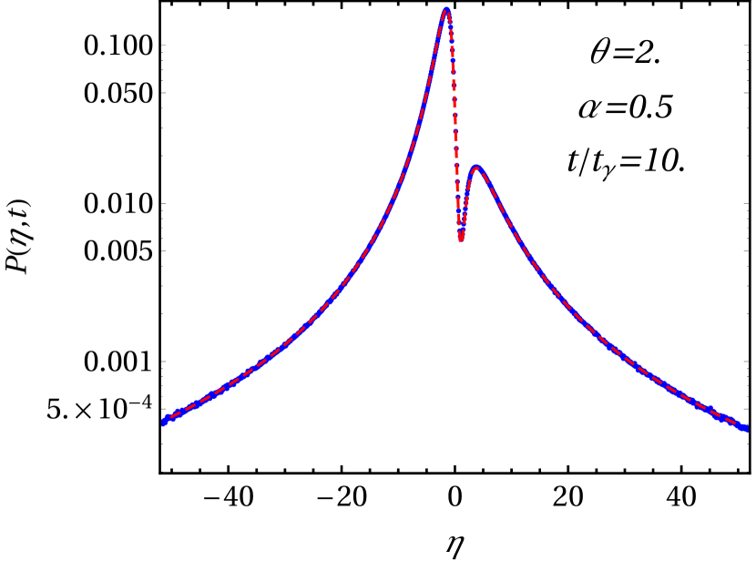
Figure 6: Distribution of stochastic efficiency $P(\eta,t)$ is plotted against the stochastic efficiency $\eta$ for $\theta=2$ and $\alpha=0.5$ at time $t/t_{\gamma}=10$. Red dashed lines plotted for analytical expression given in Eq. (62) while the blue dots are for the numerical simulation.

Note that the point $(\theta,\alpha)$ we have chosen lies in the region (see Figs. 2 and 5) where $g(\lambda_{1},\lambda_{2})$ has singularities. Figure 6 shows very good agreement between numerical simulation and theoretical prediction.

V.6 Numerical simulation: Possibility II

We compare the numerical simulation for the distribution of stochastic efficiency with the result obtained by the numerical saddle-point integration explained in Sec. V.4, for $\theta=3.0$ and $\alpha=0.5$ at time $t/t_{\gamma}=50$.

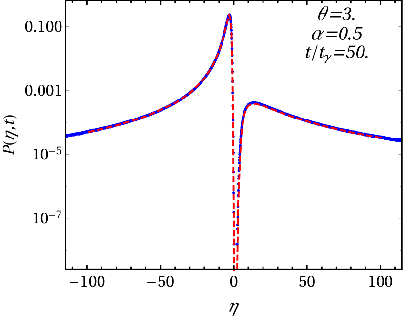
Figure 7: Distribution of stochastic efficiency $P(\eta,t)$ is plotted against the stochastic efficiency $\eta$ for $\theta=3$ and $\alpha=0.5$ at time $t/t_{\gamma}=50$. The red dashed line is plotted for the distribution $P(\eta,t)$ evaluated numerically as explained in Sec. V.4 while the blue dots correspond to the numerical simulation.

Figure 7 shows that there is nice agreement between numerical simulation and theoretical prediction.

VI Summary

We have considered a microscopic engine in which a Brownian particle is coupled to a heat bath at a constant temperature, and two external time-dependent forces, called load force and drive force, are applied to the particle. Both forces are assumed to be uncorrelated and stochastic Gaussian noises. The function of the drive force is to drive the Brownian particle against the load force. Work done by the load force and the drive force, $W_{1}$ and $W_{2}$, respectively, is stochastic quantities. Hence, the efficiency of the engine, which is the ratio of output work to the input work, $\eta=-W_{1}/W_{2}$, is also a stochastic quantity. In this paper, we have computed the distribution of stochastic efficiency $P(\eta,t)$ for large $t$.

To compute $P(\eta,t)$, we have first computed the characteristic function $\langle e^{-\lambda_{1}W_{1}-\lambda_{2}W_{2}}\rangle\sim g(\lambda_{1},\lambda_{2})\ e^{(t/t_{\gamma})\mu(\lambda_{1},\lambda_{2})}$. The asymptotic form of the joint distribution $P_{t}(W_{1},W_{2})$ for large $t$ is usually obtained by inverting the characteristic function using a saddle-point approximation. We have found that $g(\lambda_{1},\lambda_{2})$ can have singularities within the domain where the saddle point lies, and in that case we have computed the asymptotic distribution $P_{t}(W_{1},W_{2})$ by taking the singularities into account. Whether $g(\lambda_{1},\lambda_{2})$ has singularities or not depends on the choice of the parameters $\theta$ and $\alpha$ (see Fig. 2), which describe the strengths of the external forces relative to each other as well as to the strength of the thermal noise.

Using $P_{t}(W_{1},W_{2})$, we have finally computed $P(\eta,t)$, which have the large deviation form $P(\eta,t)\sim\exp[(t/t_{\gamma})\,J(\eta)]$. The large deviation function $J(\eta)$ shows two extrema: a minimum $\eta^{*}$ corresponds to an analog of Carnot efficiency while the maximum $\bar{\eta}$ is at the most probable efficiency.

As a final remark, since the random external forcing can be realized in an experimental setup Gomez-Solano et al. (2010), it would be interesting to compare the theoretical results obtained here with experiments.

Appendix A Singularity contour

The singularity contour given in Eq. (51), can be written in parametric representation as

$$\lambda_{1}(\Phi) = \dfrac{1}{1+\theta+\theta\alpha^{2}}\bigg{(}1+\sqrt{1+\alpha^{2}}\cos\Phi\bigg{)}$$

$$\lambda_{2}(\Phi) = \dfrac{1}{1+\theta+\theta\alpha^{2}}\bigg{(}1+\dfrac{\sqrt{1+\alpha^{2}}}{\alpha}\sin\Phi\bigg{)}$$ (74)

where $\Phi\in(\Phi_{-},\Phi_{+})$.

When singularity contour given by Eq. (51), intersects the boundary of domain $\mathbb{R}_{1}$, we get,

$$f^{-}(\lambda_{1}(\phi_{\pm}),\lambda_{2}(\phi_{\pm})) =0,$$ (75)

$$\cos\phi_{\pm}+A\sin\phi_{\pm}-B =0,$$ (76)

where

$$A =\alpha\sqrt{1+\theta+\theta\alpha^{2}},$$ (77)

$$B =\sqrt{(1+\alpha^{2}\theta)/[\theta(1+\theta+\theta\alpha^{2})]}(1-\theta-\theta\alpha^{2}).$$ (78)

In Eq. (76), we have used $\nu\big{(}\lambda_{1}(\phi_{\pm}),\lambda_{2}(\phi_{\pm})\big{)}=0$.

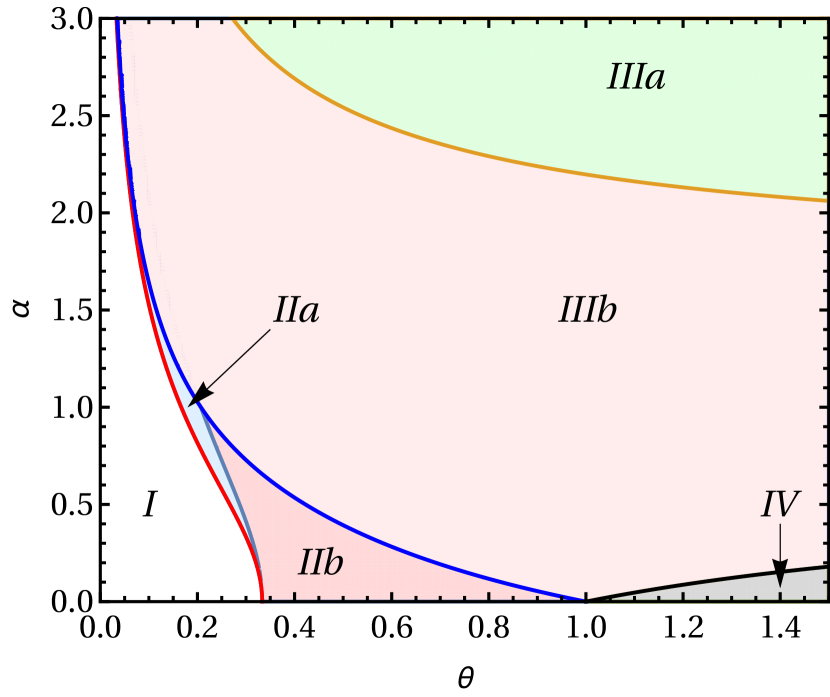
Figure 8: Phase diagram indicates the sign of $C_{1,2}^{\pm}$. Region I: $g(\lambda_{1},\lambda_{2})$ is analytic. In subregions IIa: $C_{1,2}^{\pm}>0$. In subregion IIb: $C_{1,2}^{+}>0$, $C_{1}^{-}<0$ and $C_{2}^{-}>0$. In subregion IIIa: $C_{1,2}^{+}<0$, $C_{1}^{-}<0$ and $C_{2}^{-}>0$. In subregion IIIb: $C_{1}^{+}>0$, $C_{2}^{+}<0$ , $C_{1}^{-}<0$ and $C_{2}^{-}>0$. In region IV: $C_{1}^{+}>0$, $C_{2}^{+}<0$ and $C_{1,2}^{-}<0$.

Consider $\sin\phi_{\pm}=x$; therefore Eq. (76) becomes

$$\pm\sqrt{1-x^{2}}=-Ax+B.$$ (79)

The solution of Eq. (79) is given by

$$x_{\pm}=\dfrac{AB\pm\sqrt{1+A^{2}-B^{2}}}{A^{2}+1}.$$ (80)

Since $x_{\pm}$ is a real number, therefore, $1+A^{2}-B^{2}=-1+3(1+\alpha^{2})\theta\geq 0$. Thus,

$$-1+3(1+\alpha^{2})\theta\geq 0$$ (81)

gives us the restriction on $\alpha$ and $\theta$ for which the singularity contours appears in the scenario as shown in Fig. 1(b). Using above inequality, we have plotted the phase diagram shown in Fig. 2. $x_{\pm}$ is the solution of equation $+\sqrt{1-x^{2}}=-Ax+B$ when

$$(1)\quad\quad B\geq+A\sqrt{1+A^{2}-B^{2}}\quad\quad\quad\text{for}\quad\quad\quad x_{+},$$ (82)

$$(2)\quad\quad B\geq-A\sqrt{1+A^{2}-B^{2}}\quad\quad\quad\text{for}\quad\quad\quad x_{-}.$$ (83)

Similarly, $x_{\pm}$ is the solution of equation $-\sqrt{1-x^{2}}=-Ax+B$ when

$$(3)\quad\quad B \leq+A\sqrt{1+A^{2}-B^{2}}\quad\quad\quad\text{for}\quad\quad\quad x_{+},$$ (84)

$$(4)\quad\quad B \leq-A\sqrt{1+A^{2}-B^{2}}\quad\quad\quad\text{for}\quad\quad\quad x_{-}.$$ (85)

Therefore, using $x_{\pm}$ and conditions $(1)-(4)$, one can find the end points of the contour $\lambda_{1,2}(\phi_{\pm})$.

A.1 Range of $\Phi$

Comparing $\lambda_{1,2}(\Phi_{\pm})=\lambda_{1,2}(\phi_{\pm})$, we get

$$\sin\Phi_{\pm}=C_{1}^{\pm}\quad\quad\text{and}\quad\quad\cos\Phi_{\pm}=C_{2}^{\pm},$$ (86)

where

$$C_{1}^{\pm} =\dfrac{\alpha}{\sqrt{1+\alpha^{2}}}[(1+\theta+\theta\alpha^{2})\lambda_{2}(\phi_{\pm})-1],$$ (87)

$$\quad C_{2}^{\pm} =\dfrac{1}{\sqrt{1+\alpha^{2}}}[(1+\theta+\theta\alpha^{2})\lambda_{1}(\phi_{\pm})-1],$$ (88)

with $(C_{1}^{\pm})^{2}+(C_{2}^{\pm})^{2}=1$. Using Eq. (86), one can find the restriction on $\Phi$, which is given as

$$\Phi_{\pm}=-i\ln[C_{2}^{\pm}+iC_{1}^{\pm}].$$ (89)

The sign of $C_{1,2}^{\pm}$ can be anything. Based on the sign, it is decided in which quadrant $\Phi_{\pm}$ are. Depending upon the sign, we modified the phase diagram Fig. 2 as shown in Fig. 8.

Given $\Phi_{\pm}$, one can use Eq. (74) to plot the singularity contour in $(\lambda_{1},\lambda_{2})$ plane. It is important to note that the sense of direction is always taken as $\Phi_{-}$ to $\Phi_{+}$ (anti-clockwise). Therefore, the end points of the singularity contour are given by $\lambda_{1,2}^{\pm}=\lambda_{1,2}(\Phi_{\pm})$.

References

- Callen (1985) H. B. Callen, Thermodynamics and an Introduction to Thermostatistics (Wiley, 1985), 2nd ed.
- Zemansky (1968) M. W. Zemansky, Heat and Thermodynamics (McGraw-Hill, 1968), 5th ed.
- Alberts et al. (2014) B. Alberts, A. Johnson, J. Lewis, D. Morgan, M. Raff, K. Roberts, and P. Walter, Molecular Biology of the Cell (Garland Science, 2014), 6th ed.
- Sugawa et al. (2016) M. Sugawa, K. Okazaki, M. Kobayashi, T. Matsui, G. Hummer, T. Masaike, and T. Nishizaka, Proc. Natl. Acad. Sci. 113, E2916 (2016).
- Lau et al. (2007) A. W. C. Lau, D. Lacoste, and K. Mallick, Phys. Rev. Lett. 99, 158102 (2007).
- Gelles and Landick (1998) J. Gelles and R. Landick, Cell 93, 13 (1998), ISSN 0092-8674.
- Kinosita et al. (2000) K. Kinosita, R. Yasuda, H. Noji, and K. Adachi, Phil. Trans. R. Soc. 355, 473 (2000), ISSN 0962-8436.
- Bustamante et al. (2001) C. Bustamante, D. Keller, and G. Oster, Acc. Chem. Res. 34, 412 (2001).
- Blickle and Bechinger (2012) V. Blickle and C. Bechinger, Nat. Phys. 8, 143 (2012).
- Martinez et al. (2016) I. Martinez, E. Roldan, L. Dinis, D. Petrov, J. M. R. Parrondo, and R. A. Rica, Nat. Phys. 12, 67 (2016).
- Krishnamurthy et al. (2016) S. Krishnamurthy, S. Ghosh, D. Chatterji, R. Ganapathy, and A. K. Sood, Nat. Phys. 12, 1134 (2016).
- Saira et al. (2012) O.-P. Saira, Y. Yoon, T. Tanttu, M. Möttönen, D. V. Averin, and J. P. Pekola, Phys. Rev. Lett. 109, 180601 (2012).
- Toyabe et al. (2010) S. Toyabe, T. Sagawa, M. Ueda, E. Muneyuki, and M. Sano, Nat. Phys. 6, 988 (2010).
- Ciliberto et al. (2013) S. Ciliberto, A. Imparato, A. Naert, and M. Tanase, Phys. Rev. Lett. 110, 180601 (2013).
- Collin et al. (2005) D. Collin, F. Ritort, C. Jarzynski, S. B. Smith, I. J. Tinoco, and C. Bustamante, Nat. Phys. 437, 231 (2005).
- Ciliberto et al. (2010) S. Ciliberto, S. Joubaud, and A. Petrosyan, Journal of Statistical Mechanics: Theory and Experiment 2010, P12003 (2010).
- Gomez-Solano et al. (2011) J. R. Gomez-Solano, A. Petrosyan, and S. Ciliberto, Phys. Rev. Lett. 106, 200602 (2011).
- Sabhapandit (2012) S. Sabhapandit, Phys. Rev. E 85, 021108 (2012).
- Sabhapandit (2011) S. Sabhapandit, EPL (Europhysics Letters) 96, 20005 (2011).
- Pal and Sabhapandit (2013) A. Pal and S. Sabhapandit, Phys. Rev. E 87, 022138 (2013).
- Pal and Sabhapandit (2014) A. Pal and S. Sabhapandit, Phys. Rev. E 90, 052116 (2014).
- Verley et al. (2014a) G. Verley, C. V. den Broeck, and M. Esposito, New Journal of Physics 16, 095001 (2014a).
- van Zon and Cohen (2003a) R. van Zon and E. G. D. Cohen, Phys. Rev. Lett. 91, 110601 (2003a).
- van Zon and Cohen (2003b) R. van Zon and E. G. D. Cohen, Phys. Rev. E 67, 046102 (2003b).
- van Zon and Cohen (2004) R. van Zon and E. G. D. Cohen, Phys. Rev. E 69, 056121 (2004).
- Wang et al. (2002) G. M. Wang, E. M. Sevick, E. Mittag, D. J. Searles, and D. J. Evans, Phys. Rev. Lett. 89, 050601 (2002).
- Visco (2006) P. Visco, Journal of Statistical Mechanics: Theory and Experiment 2006, P06006 (2006).
- Kundu et al. (2011) A. Kundu, S. Sabhapandit, and A. Dhar, Journal of Statistical Mechanics: Theory and Experiment 2011, P03007 (2011).
- Farago (2002) J. Farago, Journal of Statistical Physics 107, 781 (2002), ISSN 1572-9613.
- Gupta and Sabhapandit (2016) D. Gupta and S. Sabhapandit, EPL 115, 60003 (2016).
- Sekimoto (1997) K. Sekimoto, Journal of the Physical Society of Japan 66, 1234 (1997).
- Seifert (2005) U. Seifert, Phys. Rev. Lett. 95, 040602 (2005).
- Seifert (2008) U. Seifert, The European Physical Journal B 64, 423 (2008), ISSN 1434-6036.
- Evans et al. (1993) D. J. Evans, E. G. D. Cohen, and G. P. Morriss, Phys. Rev. Lett. 71, 2401 (1993).
- Evans and Searles (1994) D. J. Evans and D. J. Searles, Phys. Rev. E 50, 1645 (1994).
- Searles and Evans (2000) D. J. Searles and D. J. Evans, The Journal of Chemical Physics 113, 3503 (2000).
- Searles and Evans (2001) D. J. Searles and D. J. Evans, International Journal of Thermophysics 22, 123 (2001), ISSN 1572-9567.
- Gallavotti and Cohen (1995) G. Gallavotti and E. G. D. Cohen, Phys. Rev. Lett. 74, 2694 (1995).
- Kurchan (1998) J. Kurchan, Journal of Physics A: Mathematical and General 31, 3719 (1998).
- Lebowitz and Spohn (1999) J. L. Lebowitz and H. Spohn, Journal of Statistical Physics 95, 333 (1999), ISSN 1572-9613.
- Crooks (1998) G. E. Crooks, Journal of Statistical Physics 90, 1481 (1998), ISSN 1572-9613.
- Crooks (1999) G. E. Crooks, Phys. Rev. E 60, 2721 (1999).
- Crooks (2000) G. E. Crooks, Phys. Rev. E 61, 2361 (2000).
- Touchette (2009) H. Touchette, Physics Reports 478, 1 (2009), ISSN 0370-1573.
- Verley et al. (2014b) G. Verley, M. Esposito, T. Willaert, and C. Van den Broeck, Nat. Commun. 5, 4721 (2014b).
- Verley et al. (2014c) G. Verley, T. Willaert, C. Van den Broeck, and M. Esposito, Phys. Rev. E 90, 052145 (2014c).
- Gingrich et al. (2014) T. R. Gingrich, G. M. Rotskoff, S. Vaikuntanathan, and P. L. Geissler, New Journal of Physics 16, 102003 (2014).
- Polettini et al. (2015) M. Polettini, G. Verley, and M. Esposito, Phys. Rev. Lett. 114, 050601 (2015).
- Proesmans et al. (2015) K. Proesmans, B. Cleuren, and C. V. den Broeck, EPL (Europhysics Letters) 109, 20004 (2015).
- Proesmans and den Broeck (2015) K. Proesmans and C. V. den Broeck, New Journal of Physics 17, 065004 (2015).
- Proesmans et al. (2016a) K. Proesmans, Y. Dreher, M. c. v. Gavrilov, J. Bechhoefer, and C. Van den Broeck, Phys. Rev. X 6, 041010 (2016a).
- Benenti et al. (2011) G. Benenti, K. Saito, and G. Casati, Phys. Rev. Lett. 106, 230602 (2011).
- Shiraishi et al. (2016) N. Shiraishi, K. Saito, and H. Tasaki, Phys. Rev. Lett. 117, 190601 (2016).
- Proesmans et al. (2016b) K. Proesmans, B. Cleuren, and C. Van den Broeck, Phys. Rev. Lett. 116, 220601 (2016b).
- Park et al. (2016) J.-M. Park, H.-M. Chun, and J. D. Noh, Phys. Rev. E 94, 012127 (2016).
- Lee et al. (2013) J. S. Lee, C. Kwon, and H. Park, Phys. Rev. E 87, 020104 (2013).
- Noh (2014) J. D. Noh, Journal of Statistical Mechanics: Theory and Experiment 2014, P01013 (2014).
- Gomez-Solano et al. (2010) J. R. Gomez-Solano, L. Bellon, A. Petrosyan, and S. Ciliberto, EPL (Europhysics Letters) 89, 60003 (2010).