The Complexity Landscape of
Fixed-Parameter Directed Steiner Network Problems

Abstract

Given a directed graph $G$ and a list $(s_{1},t_{1})$, $\dots$, $(s_{d},t_{d})$ of terminal pairs, the Directed Steiner Network problem asks for a minimum-cost subgraph of $G$ that contains a directed $s_{i}\to t_{i}$ path for every $1\leq i\leq d$. The special case Directed Steiner Tree (when we ask for paths from a root $r$ to terminals $t_{1}$, $\dots$, $t_{d}$) is known to be fixed-parameter tractable parameterized by the number of terminals, while the special case Strongly Connected Steiner Subgraph (when we ask for a path from every $t_{i}$ to every other $t_{j}$) is known to be W[1]-hard parameterized by the number of terminals. We systematically explore the complexity landscape of directed Steiner problems to fully understand which other special cases are FPT or W[1]-hard. Formally, if ${\mathcal{H}}$ is a class of directed graphs, then we look at the special case of Directed Steiner Network where the list $(s_{1},t_{1})$, $\dots$, $(s_{d},t_{d})$ of demands form a directed graph that is a member of ${\mathcal{H}}$. Our main result is a complete characterization of the classes ${\mathcal{H}}$ resulting in fixed-parameter tractable special cases: we show that if every pattern in ${\mathcal{H}}$ has the combinatorial property of being “transitively equivalent to a bounded-length caterpillar with a bounded number of extra edges,” then the problem is FPT, and it is W[1]-hard for every recursively enumerable ${\mathcal{H}}$ not having this property. This complete dichotomy unifies and generalizes the known results showing that Directed Steiner Tree is FPT [Dreyfus and Wagner, Networks 1971], $q$-Root Steiner Tree is FPT for constant $q$ [Suchý, WG 2016], Strongly Connected Steiner Subgraph is W[1]-hard [Guo et al., SIAM J. Discrete Math. 2011], and Directed Steiner Network is solvable in polynomial-time for constant number of terminals [Feldman and Ruhl, SIAM J. Comput. 2006], and moreover reveals a large continent of tractable cases that were not known before.

1 Introduction

Steiner Tree is a basic and well-studied problem of combinatorial optimization: given an edge-weighted undirected graph $G$ and a set $R\subseteq V(G)$ of terminals, it asks for a minimum-cost tree connecting the terminals. The problem is well known to be NP-hard, in fact, it was one of the 21 NP-hard problems identified by Karp’s seminal paper [29]. There is a large literature on approximation algorithms for Steiner Tree and its variants, resulting for example in constant-factor approximation algorithms for general graphs and approximation schemes for planar graphs [7, 17, 9, 5, 4, 3, 2, 8, 33, 32, 30, 1, 20, see]. From the viewpoint of parameterized algorithms, the first result is the classic dynamic-programming algorithm of Dreyfus and Wagner [20] from 1971, which solves the problem with $k=|R|$ terminals in time $3^{k}\cdot n^{O(1)}$. This shows that the problem is fixed-parameter tractable [16, 19] (FPT) parameterized by the number of terminals, i.e., there is an algorithm to solve the problem in time $f(k)\cdot n^{O(1)}$ for some computable function $f$. In this paper we will only be concerned with this well-studied parameter $k=|R|$. A more recent algorithm by Fuchs et al. [26] obtains runtime $(2+\delta)^{k}\cdot n^{O(1)}$ for any constant $\delta>0$. For graphs with polynomial edge weights the running time was improved to $2^{k}\cdot n^{O(1)}$ by Nederlof [31] using the technique of fast subset convolution. Steiner Forest is the generalization where the input contains an edge-weighted graph $G$ and a list $(s_{1},t_{1}),\dots,(s_{d},t_{d})$ of pairs of terminals and the task is to find a minimum-cost subgraph containing an $s_{i}$–$t_{i}$ path for every $1\leq i\leq d$. The observation that the connected components of the solution to Steiner Forest induces a partition on the set $R=\{s_{1},\dots,s_{d},t_{1},\dots,t_{d}\}$ of terminals such that each class of the partition forms a tree, implies the fixed-parameter tractability of Steiner Forest parameterized by $k=|R|$: we can solve the problem by for example trying every partition of $R$ and invoking a Steiner Tree algorithm for each class of the partition.

On directed graphs, Steiner problems can become significantly harder, and while there is a richer landscape of variants, only few results are known [28, 11, 22, 10, 35, 15, 14, 13, 21]. A natural and well-studied generalization of Steiner Tree to directed graphs is Directed Steiner Tree (DST), where an arc-weighted directed graph $G$ and terminals $r,t_{1},\dots,t_{d}$ are given and the task is to find a minimum-cost subgraph containing an $r\to t_{i}$ path for every $1\leq i\leq d$. Using essentially the same techniques as in the undirected case [31, 26, 20], one can show that this problem is also FPT parameterized by the number of terminals $k=d+1$. An equally natural generalization of Steiner Tree to directed graphs is the Strongly Connected Steiner Subgraph (SCSS) problem, where an arc-weighted directed graph $G$ with terminals $t_{1},\dots,t_{k}$ is given, and the task is to find a minimum-cost subgraph containing a $t_{i}\to t_{j}$ path for any $1\leq i,j\leq k$ with $i\neq j$. Guo et al. [28] showed that, unlike DST, the SCSS problem is W[1]-hard parameterized by $k$ (see also [15]), and is thus unlikely to be FPT for this parameter (for more background on parameterized complexity theory see [25]). A common generalization of DST and SCSS is the Directed Steiner Network (DSN) problem (also called Directed Steiner Forest or Point-to-Point Connection), where an arc-weighted directed graph $G$ and a list $(s_{1},t_{1}),\dots,(s_{d},t_{d})$ of terminal pairs are given and the task is to find a minimum-cost subgraph containing an $s_{i}\to t_{i}$ path for every $1\leq i\leq d$. Being a generalization of SCSS, the Directed Steiner Network problem is also W[1]-hard for the number of terminals $k$ in the set $R=\{s_{1},\dots,s_{d},t_{1},\dots,t_{d}\}$, but Feldman and Ruhl [22] showed that the problem is solvable in time $n^{O(d)}$, that is, in polynomial time for every constant $d=O(k^{2})$.

Besides Directed Steiner Tree, what other special cases of Directed Steiner Network are fixed-parameter tractable? Our main result gives a complete map of the complexity landscape of directed Steiner problems on general input graphs, precisely describing all the FPT/W[1]-hard variants and revealing highly non-trivial generalizations of Directed Steiner Tree that are still tractable. Our results are expressed in the following formal framework. The pairs $(s_{1},t_{1}),\dots,(s_{d},t_{d})$ in the input of DSN can be interpreted as a directed (unweighted) pattern graph on a set $R$ of terminals. If this pattern graph is an out-star, then the problem is precisely DST; if it is a bidirected clique, then the problem is precisely SCSS. More generally, if ${\mathcal{H}}$ is any class of graphs, then we define the Directed Steiner ${\mathcal{H}}$-Network (${\mathcal{H}}$-DSN) problem as the restriction of DSN where the pattern graph is a member of ${\mathcal{H}}$. That is, the input of ${\mathcal{H}}$-DSN is an arc-weighted directed graph $G$, a set $R\subseteq V(G)$ of terminals, and an unweighted directed graph $H\in{\mathcal{H}}$ on $R$; the task is to find a minimum-cost subgraph $N\subseteq G$ (“network”) such that $N$ contains an $s\to t$ path for every $st\in E(H)$.

We give a complete characterization of the classes ${\mathcal{H}}$ for which ${\mathcal{H}}$-DSN is FPT or W[1]-hard. We need the following definition of “almost-caterpillar graphs” to describe the borderline between the easy and hard cases (see Figure 1).

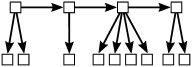
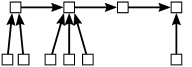
Figure 1: Two $4$-caterpillars: an out-caterpillar (on the left) and an in-caterpillar (on the right).

Definition .

A $\lambda_{0}$-caterpillar graph is constructed as follows. Take a directed path $(v_{1},\ldots,v_{\lambda_{0}})$ from $v_{1}$ to $v_{\lambda_{0}}$, and let $W_{1},\ldots,W_{\lambda_{0}}$ be pairwise disjoint vertex sets such that $v_{i}\in W_{i}$ for each $i\in\{1,\ldots,\lambda_{0}\}$. Now add edges such that either every $W_{i}$ forms an out-star with root $v_{i}$, or every $W_{i}$ forms an in-star with root $v_{i}$. In the former case we also refer to the resulting $\lambda_{0}$-caterpillar as an out-caterpillar, and in the latter as an in-caterpillar. A $0$-caterpillar is the empty graph. The class ${\mathcal{C}}_{\lambda,\delta}$ contains all directed graphs $H$ such that there is a set of edges $F\subseteq E(H)$ of size at most $\delta$ for which the remaining edges $E(H)\setminus F$ span a $\lambda_{0}$-caterpillar for some $\lambda_{0}\leq\lambda$.

If there is an $s\to t$ path in the pattern graph $H$ for two terminals $s,t\in R$, then adding the edge $st$ to $H$ does not change the problem: connectivity from $s$ to $t$ is already implied by $H$, hence adding this edge does not change the feasible solutions. That is, adding a transitive edge does not change the solution space and hence it is really only the transitive closure of the pattern $H$ that matters. We say that two pattern graphs are transitively equivalent if their transitive closures are isomorphic. We denote the class of patterns that are transitively equivalent to some pattern of ${\mathcal{C}}_{\lambda,\delta}$ by ${\mathcal{C}}^{*}_{\lambda,\delta}$. Our main result is a sharp dichotomy saying that ${\mathcal{H}}$-DSN is FPT if every pattern of ${\mathcal{H}}$ is transitively equivalent to an almost-caterpillar graph and it is W[1]-hard otherwise. In order to provide reductions for the hardness results we need the technical condition that the class of patterns is recursively enumerable, i.e., there is some algorithm, which enumerates all members of the class. In the FPT cases, we make the algorithmic result more precise by stating a running time that is expressed as a function of $\lambda$, $\delta$, and the vertex cover number $\tau$ of the input pattern $H$, i.e., $\tau$ is the size of the smallest vertex subset $W$ of $H$ such that every edge of $H$ is incident to a vertex of $W$.

Theorem 1.1.

Let ${\mathcal{H}}$ be a recursively enumerable class of patterns.

1. If there are constants $\lambda$ and $\delta$ such that ${\mathcal{H}}\subseteq{\mathcal{C}}^{*}_{\lambda,\delta}$, then ${\mathcal{H}}$-DSN with parameter $k=|R|$ is FPT and can be solved in $2^{O(k+\tau\omega\log\omega)}n^{O(\omega)}$ time, where $\omega=(1+\lambda)(\lambda+\delta)$ and $\tau$ is the vertex cover number of the given input pattern $H\in{\mathcal{H}}$.

2. Otherwise, if there are no such constants $\lambda$ and $\delta$, then the problem is W[1]-hard for parameter $k$.

In Theorem 1.1(1), the reason for the slightly complicated runtime is that the algorithm was optimized to match the runtime of some previous algorithms in special cases. In particular, invoking Theorem 1.1 with specific classes ${\mathcal{H}}$, we can obtain algorithmic or hardness results for specific problems. For example, we may easily recover the following facts:

• If ${\mathcal{H}}_{\textup{DST}}$ is the class of all out-stars, then ${\mathcal{H}}_{\textup{DST}}$-DSN is precisely the DST problem. As ${\mathcal{H}}_{\textup{DST}}\subseteq{\mathcal{C}}^{*}_{1,0}$ holds, Theorem 1.1(1) recovers the fact that DST can be solved in time $2^{O(k)}n^{O(1)}$ and is hence FPT parameterized by the number $k$ of terminals [31, 26, 20].

• If ${\mathcal{H}}_{\textup{SCSS}}$ is the class of all bidirected cliques (or equivalently the class of all directed cycles), then ${\mathcal{H}}_{\textup{SCSS}}$-DSN is precisely the SCSS problem. One can observe that ${\mathcal{H}}_{\textup{SCSS}}$ is not contained in ${\mathcal{C}}^{*}_{\lambda,\delta}$ for any constants $\lambda,\delta$ (for example, because every graph in ${\mathcal{C}}_{\lambda,\delta}$ has at most $\lambda+2\delta$ vertices with both positive in-degree and positive out-degree, and this remains true also for the graphs in ${\mathcal{C}}^{*}_{\lambda,\delta}$). Hence Theorem 1.1(2) recovers the fact that SCSS is W[1]-hard [28]. Note that any pattern of ${\mathcal{H}}_{\textup{SCSS}}$ is transitively equivalent to a bidirected star with less than $2k$ edges, so that ${\mathcal{H}}_{\textup{SCSS}}\subseteq{\mathcal{C}}^{*}_{0,2k}$. Since a star has vertex cover number $\tau=1$, for SCSS our algorithm in Theorem 1.1(1) recovers the running time of $2^{O(k\log k)}n^{O(k)}=n^{O(k)}$ given by Feldman and Ruhl [22]. We note however, that the constants in the degree of the polynomial are larger in our case compared to [22].

• Let ${\mathcal{H}}_{d}$ be the class of directed graphs with at most $d$ edges. As ${\mathcal{H}}_{d}\subseteq{\mathcal{C}}^{*}_{0,d}$ holds, Theorem 1.1(1) recovers the fact that Directed Steiner Network with at most $d$ demands is polynomial-time solvable for every constant $d$ [22].

• Recently, Suchý [34] studied the following generalization of DST and SCSS: in the $q$-Root Steiner Tree ($q$-RST) problem, a set of $q$ roots and a set of leaves are given, and the task is to find a minimum-cost network where the roots are in the same strongly connected component and every leaf can be reached from every root. Building on the work of Feldman and Ruhl [22], Suchý [34] presented an algorithm with running time $2^{O(k)}\cdot n^{O(q)}$ for this problem, which shows that it is FPT for every constant $q$. Let ${\mathcal{H}}_{\textup{$q$-RST}}$ be the class of directed graphs that are obtained from an out-star by making $q-1$ of the edges bidirected. Observe that ${\mathcal{H}}_{\textup{$q$-RST}}$ is a subset of ${\mathcal{C}}_{1,q-1}$, that $q$-RST can be expressed by an instance of ${\mathcal{H}}_{\textup{$q$-RST}}$-DSN, and that any pattern of ${\mathcal{H}}_{\textup{$q$-RST}}$ has vertex cover number $\tau=1$. Thus Theorem 1.1(1) implies that $q$-RST can be solved in time $2^{O(k+q\log q)}\cdot n^{O(q)}=2^{O(k)}\cdot n^{O(q)}$, recovering the fact that it is FPT for every constant $q$.

Thus the algorithmic side of Theorem 1.1 unifies and generalizes three algorithmic results: the fixed-parameter tractability of DST (which is based on dynamic programming on the tree structure of the solution), $q$-RST (which is based on simulating a “pebble game”), but also the polynomial-time solvability of DSN with constant number of demands (which also is based on simulating a “pebble game”). Let us point out that our algorithmic results are significantly more general than just the unification of these three results: the generalization from stars to bounded-length caterpillars is already a significant extension and very different from earlier results. We consider it a major success of the systematic investigation that, besides finding the unifying algorithmic ideas generalizing all previous results, we were able to find tractable special cases in an unexpected new direction.

There is a surprising non-monotonicity in the classification result of Theorem 1.1. As DST is FPT and SCSS is W[1]-hard, one could perhaps expect that ${\mathcal{H}}$-DSN becomes harder as the pattern become denser. However, it is possible that the addition of further demands makes the problem easier. For example, if ${\mathcal{H}}$ contains every graph that is the vertex-disjoint union of two out-stars, then ${\mathcal{H}}$-DSN is classified to be W[1]-hard by Theorem 1.1(2). However, if we consider those graphs where there is also a directed edge from the center of one star to the other star, then these graphs are 2-caterpillars (i.e., contained in ${\mathcal{C}}_{2,0}$) and hence ${\mathcal{H}}$-DSN becomes FPT by Theorem 1.1(1). This unexpected non-monotonicity further underlines the importance of completely mapping the complexity landscape of the problem area: without complete classification, it would be very hard to predict what other tractable/intractable special cases exist.

We mention that one can also study the vertex-weighted version of the problem, where the input graph has weights on the vertices and the goal is to minimize the total vertex-weight of the solution. In general, vertex-weighted problems can be more challenging than edge-weighted variants [17, 5, 30, 12]. However, for general directed graphs, there are easy transformations between the two variants. Thus the results of this paper can be interpreted for the vertex-weighted version as well.

1.1 Our techniques

We prove Theorem 1.1 the following way. In Section 2, we first establish the combinatorial bound that there is a solution whose cutwidth, and hence also (undirected) treewidth, is bounded by the number of demands.

Theorem 1.2.

A minimal solution $M$ to a pattern $H$ has cutwidth at most $7d$ if $d=|E(H)|$.

This serves as the first step, which we exploit in Section 3 to prove that if the pattern is an almost-caterpillar in ${\mathcal{C}}^{*}_{\lambda,\delta}$, then the (undirected) treewidth of the optimum solution can be bounded by a function of $\lambda$ and $\delta$.

Theorem 1.3.

The treewidth of a minimal solution to any pattern graph in ${\mathcal{C}}^{*}_{\lambda,\delta}$ is at most $7(1+\lambda)(\lambda+\delta)$.

To prove the above two theorems we thoroughly analyze the combinatorial structure of minimal solutions, by untangling the intricate interplay between the $s\to t$ paths in a given solution for demands $st$ of a pattern graph $H$. The resulting bounds can then be exploited in an algorithm that restricts the search for a bounded-treewidth solution (Section 4). To obtain this algorithm we generalize dynamic programming techniques for other settings to the DSN case, by introducing novel tools to tackle the intricacies of this problem.

Theorem 1.4.

Let an instance of ${\mathcal{H}}$-DSN be given by a graph $G$ with $n$ vertices, and a pattern $H$ on $k$ terminals with vertex cover number $\tau$. If the optimum solution to $H$ in $G$ has treewidth $\omega$, then the optimum can be computed in $2^{O(k+\tau\omega\log\omega)}n^{O(\omega)}$ time.

Combining Theorem 1.3 and Theorem 1.4 proves the algorithmic side of Theorem 1.1. We remark that the proof is completely self-contained (with the exception of some basic facts on treewidth) and in particular we do not build on the algorithms of Feldman and Ruhl [22]. As combining Theorem 1.2 and Theorem 1.4 already proves that DSN with a constant number of demands can be solved in polynomial time, as a by-product this gives an independent proof for the result of Feldman and Ruhl [22]. One can argue which algorithm is simpler, but perhaps our proof (with a clean split of a combinatorial and an algorithmic statement) is more methodological and better reveals the underlying reason why the problem is tractable.

Finally, in Section 5 we show that whenever the patterns in ${\mathcal{H}}$ are not transitively equivalent to almost-caterpillars, the problem is W[1]-hard. Our proof follows a novel, non-standard route. We first show that there is only a small number of obstacles for not being transitively equivalent to almost-caterpillars: the graph class contains (possibly after identification of vertices) arbitrarily large strongly connected graphs, pure diamonds, or flawed diamonds (see Section 5.2 for the precise statement). Showing the existence of these obstacles needs a non-trivial combinatorial argument. We then provide a separate W[1]-hardness proof for each of these obstacles, completing the proof of the hardness side of Theorem 1.1.

1.2 Subsequent related work

Since the publication of the conference version [23] of this paper several results have appeared that build on our work. Especially the algorithm of Theorem 1.4 has been used as a subroutine to solve several special cases of DSN. We survey some of these results here.

Parameterizing by the number $k$ of terminals.

As mentioned above, the algorithm for DSN based on simulating a “pebble game” by Feldman and Ruhl [22] has a faster runtime of $n^{O(d)}$ than implied by Theorem 1.4, where $d$ is the number of demands. Measured in the stronger parameter $k$ (which can be smaller than $d$ up to a quadratic factor) the Feldman and Ruhl [22] algorithm runs in $n^{O(k^{2})}$ time. Interestingly, Eiben et al. [21] show that this is essentially best possible, as no $f(k)n^{o(k^{2}/\log k)}$ time algorithm exists for DSN for any computable function $f$, under the Exponential Time Hypothesis (ETH). However, as summarized below, in special cases it is possible to beat this lower bound.

Planar and bounded genus graphs.

A directed graph is considered planar if its underlying undirected graph is. For such inputs Chitnis et al. [15] show that under ETH no $f(k)n^{o(k)}$ time algorithm can solve DSN. Eiben et al. [21] show that an optimum solution of genus $g$ has treewidth $2^{O(g)}k$ and thus Theorem 1.4 implies an algorithm with runtime $2^{O(k^{2}\log k)}n^{O(k)}$ for graphs of constant genus, matching the previous runtime lower bound for planar graphs. However, for the special case of the SCSS problem, Chitnis et al. [15] prove that in planar graphs there exists a faster algorithm with runtime $2^{O(k)}n^{O(\sqrt{k})}$. To obtain such an algorithm, in the conference version of [15] the authors devise a generalization of the “pebble games” of Feldman and Ruhl [22] for SCSS in planar graphs. However, in the journal version [15] the authors use Theorem 1.4 to get a much cleaner and simpler proof, by showing that any optimum solution has treewidth $O(\sqrt{k})$. They also obtain a matching runtime lower bound of $f(k)n^{o(\sqrt{k})}$ for SCSS on planar graphs.

Bidirected graphs.

An interesting application of Theorem 1.4 is the SCSS problem on bidirected graphs, i.e., directed graphs for which an edge $uv$ exists if and only if its reverse edge $vu$ also exists and has the same weight. While this problem remains NP-hard, Chitnis et al. [13] show that it is FPT parameterized by $k$, which is in contrast to general input graphs where the problem is W[1]-hard (as also implied by Theorem 1.1). To show this result, it is not enough to bound the treewidth of a solution and then apply Theorem 1.4 directly, as is done for the above mentioned problems on planar graphs. In fact, there are examples [13] in which the optimum solution to SCSS on bidirected graphs has treewidth $\Theta(k)$. Nevertheless, as shown in [13] it is possible to decompose the optimum solution to this problem into poly-trees, i.e., directed graphs of (undirected) treewidth $1$. As a consequence, an FPT algorithm can guess the decomposition of the optimum, and apply Theorem 1.4 repeatedly (with $\omega=1$) to compute all poly-tree solutions. This algorithm can be made to run in $2^{k^{2}+O(k)}n^{O(1)}$ time. In contrast, for the more general DSN problem on bidirected graphs, Chitnis et al. [13] show that no $f(k)n^{o(k/\log k)}$ time algorithm exists, under ETH.

Planar bidirected graphs.

If the input graph is both planar and bidirected, then Chitnis et al. [13] show that the treewidth of any optimum solution to DSN is $O(\sqrt{k})$. Theorem 1.4 then implies an algorithm with runtime $2^{O(k^{3/2}\log k)}n^{O(\sqrt{k})}$, which is faster than possible in planar graphs but also in bidirected graphs, as mentioned above. Furthermore, they show that Theorem 1.4 can be used to obtain a parameterized approximation scheme for DSN on planar bidirected graphs, i.e., a $(1+{\varepsilon})$-approximation can be computed in $2^{O(k^{2})}n^{2^{O(1/{\varepsilon})}}$ time. For this they prove that the optimum solution to DSN in planar bidirected graphs can be covered by a set of DSN solutions, each of which only contains $2^{O(1/{\varepsilon})}$ terminals, and such that the sum of the costs of all these solutions is only a $(1+{\varepsilon})$-fraction more than the optimum. Similar to SCSS on bidirected graphs, the idea now is to guess how these solutions cover the terminal set, and then compute all of them using the above mentioned $2^{O(k^{3/2}\log k)}n^{O(\sqrt{k})}$ time algorithm for DSN on planar bidirected graphs (which follows from Theorem 1.4). Since each of the solutions only contains $2^{O(1/{\varepsilon})}$ terminals, the degree of the polynomial depends only on ${\varepsilon}$ every time the algorithm of Theorem 1.4 is executed.

1.3 Preliminaries

In this paper, we are mainly concerned with directed graphs, i.e., graphs for which every edge is an ordered pair of vertices. For convenience, we will also give definitions, such as the treewidth, for directed graphs, even if they are usually defined for undirected graphs. For any graph $G$ we denote its vertex set by $V(G)$ and its edge set by $E(G)$. We denote a directed edge from $u$ to $v$ by $uv$, so that $u$ is its tail and $v$ is its head. We say that both $u$ and $v$ are incident to the edge $uv$, and $u$ and $v$ are adjacent if the edge $uv$ or the edge $vu$ exists. We refer to $u$ and $v$ as the endpoints of $uv$. For a vertex $v$ the in-degree (out-degree) is the number of edges that have $v$ as their head (tail). A source (target) is a vertex of in-degree $0$ (out-degree $0$). An in-arborescence (out-arborescence) is a connected graph with a unique target (source), also called its root, such that every vertex except the root has out-degree $1$ (in-degree $1$). The leaves of an in-arborescence (out-arborescence) are its sources (targets). A $u\to v$ path is an out-arborescence with root $u$ and a single leaf $v$, and its length is its number of edges. A star $S$ with root $u$ is a graph in which every edge is incident to $u$. All vertices in a star different from the root are called its leaves. An in-star (out-star) is a star which is an in-arborescence (out-arborescence). A strongly connected component (SCC) $H$ of a directed graph $G$ is an inclusion-wise maximal sub-graph of $G$ for which there is both a $u\to v$ path and a $v\to u$ path for every pair of vertices $u,v\in V(H)$. A directed acyclic graph (DAG) is a graph in which every SCC is a singleton, i.e., it contains no cycles.

The following observation is implicit in previous work (cf. [22]) and will be used throughout this paper. Here we consider a minimal solution $M$ to an instance of DSN, in which no edge can be removed without making the solution infeasible.

Lemma .

Consider an instance of DSN where the pattern $H$ is an out-star (resp., in-star) with root $t\in R$. Then any minimal solution $M$ to $H$ is an out-arborescence (resp., in-arborescence) rooted at $t$ for which every leaf is a terminal.

Proof.

We only prove the case when $H$ is an out-star, as the other case follows by symmetry. Suppose for contradiction that $M$ is not an out-arborescence. As it is clear that $M$ is connected and $t$ is the unique source in a minimal solution, $M$ not being an out-arborescence implies that there is a vertex $v\in V(M)$ with in-degree at least $2$, i.e., there are two distinct edges $e$ and $f$ of $M$ that have $v$ as their head. Since $M$ is a minimal solution, removing $e$ disconnects some terminal $\ell$ from $t$, which in particular means that there is a $t\to\ell$ path $P$ going through $e$. Clearly, this path cannot go through $f$, as both $e$ and $f$ have the same head $v$. Thus if we remove $f$, then any terminal $\ell^{\prime}$ will remain being reachable from $t$: we may reroute any $t\to\ell$ path $Q$ that passed through $f$ via a path through $e$ instead by following $P$ from $t$ to $v$, the head of $f$, and then following $Q$ from $v$ to $\ell^{\prime}$. This however contradicts the minimality of $M$. ∎

A tree decomposition $D$ of a graph $G$ is an undirected tree for which every node $w\in V(D)$ is associated with a set $b_{w}\subseteq V(G)$ called a bag. Additionally it satisfies the following properties:

1. for every edge $uv\in E(G)$ there is a bag $b_{w}$ for some $w\in V(D)$ containing it, i.e., $u,v\in b_{w}$, and

2. for every vertex $v\in V(G)$ the nodes of $D$ associated with the bags containing $v$ induce a non-empty and connected subgraph of $D$.

The width of the tree decomposition is $\max\{|b_{w}|-1\mid w\in V(D)\}$. The treewidth of a graph $G$ is the minimum width of any tree decomposition for $G$. It is known (by an easy folklore proof) that for any graph $G$ of treewidth $\omega$ there is a smooth tree decomposition $D$ of $G$, which means that $|b_{w}|=\omega+1$ for all nodes $w$ of $D$ and $|b_{w}\cap b_{w^{\prime}}|=\omega$ for all adjacent nodes $w,w^{\prime}$ of $D$.

2 The cutwidth of minimal solutions for bounded-size patterns

The goal of this section is to prove Theorem 1.2: we bound the cutwidth of a minimal solution $M$ to a pattern $H$ in terms of $d=|E(H)|$. A layout of a graph $G$ is an injective function $\psi:V(G)\rightarrow\mathbb{N}$ inducing a total order on the vertices of $G$. Given a layout, we define the set $V_{i}=\{v\in V(G)\mid\psi(v)\leq i\}$ and say that an edge crosses the cut $(V_{i},\overline{V}_{i})$ if it has one endpoint in $V_{i}$ and one endpoint in $\overline{V}_{i}:=V(G)\setminus V_{i}$. The cutwidth of the layout is the maximum number of edges crossing any cut $(V_{i},\overline{V}_{i})$ for any $i\in\mathbb{N}$. The cutwidth of a graph is the minimum cutwidth over all its layouts.

Like Feldman and Ruhl [22], we consider the two extreme cases of directed acyclic graphs (DAGs) and strongly connected components (SCCs) in our proof. Contracting all SCCs of a minimal solution $M$ without removing parallel edges sharing the same head and tail, but removing the resulting self-loops, produces a directed acyclic multi-graph $D$, the so-called condensation graph of $M$. We bound the cutwidth of $D$ and the SCCs of $M$ separately, and then put together these two bounds to obtain a bound for the cutwidth of $M$. As we will see, bounding the cutwidth of the acyclic multi-graph $D$ and putting together the bounds are fairly simple. The main technical part is bounding the cutwidth of the SCCs.

We will need two simple facts about cutwidth. First, the cutwidth of an acyclic multi-graph can be bounded using the existence of a topological ordering of the vertices. That is, for any acyclic graph $G$ there is an injective function $\varphi:V(G)\rightarrow\mathbb{N}$ such that $\varphi(u)<\varphi(v)$ if $uv\in E(G)$. Note that such a function in particular is a layout.

Lemma .

If $D$ is an acyclic directed multi-graph $D$ that is the union of $d$ paths and $\varphi_{D}$ is an arbitrary topological ordering of $D$, then the layout given by $\varphi_{D}$ has cutwidth at most $d$.

Proof.

To bound the cutwidth, we argue that a path $P$ crosses any cut $(V_{i},\overline{V}_{i})$ at most once. Note that no edge can have a head $v$ and tail $u$ with $\varphi_{D}(v)\leq\varphi_{D}(u)$, since $\varphi_{D}$ is a topological ordering. In particular, for the first edge $uv$ of $P$ crossing $(V_{i},\overline{V}_{i})$ we get $\varphi_{D}(u)\leq i<\varphi_{D}(v)$. For any vertex $w$ reachable from $v$ on the path, the transitivity of the topological order implies $i<\varphi_{D}(w)$ so that $w$ cannot be the tail of an edge crossing the cut. Thus no second edge of the path $P$ crosses $(V_{i},\overline{V}_{i})$. As $D$ is the union of $d$ paths, each cut is crossed by at most $d$ edges of $D$. ∎

The next lemma shows that bounding the cutwidth of each SCC and the condensation graph of $G$, bounds the cutwidth of $G$.

Lemma .

Let $G$ be a directed graph and $D$ be its condensation multi-graph. If the cutwidth of $D$ is $x$ and the cutwidth of every SCC of $G$ is at most $y$, then the cutwidth of $G$ is at most $x+y$.

Proof.

Let SCC$(u)\subseteq G$ be the SCC of $G$ that was contracted into the vertex $u$ in $D$. If a vertex $u$ of $G$ was not contracted, then SCC$(u)$ is the singleton $u$. For each $u\in V(D)$, there exists a layout $\varphi_{u}$ of SCC$(u)$ with cutwidth at most $y$, while for $D$ there exists a layout $\varphi_{D}$ with cutwidth at most $x$. Let $\mu=\max\{\varphi_{u}(v)\mid u\in V(D)\land v\in$ SCC$(u)\}$ be the maximum value taken by any layout of an SCC. We define a layout $\psi$ of $G$ as $\psi(v)=\mu\cdot\varphi_{D}(u)+\varphi_{u}(v)$, where $v\in$ SCC$(u)$. Since the topological orderings are injective, $\psi$ is injective, and the intervals $[\mu\cdot\varphi_{D}(u)+1,\mu\cdot\varphi_{D}(u)+\mu]$ of values that $\psi$ can take for vertices of different SCCs are disjoint. Hence for any $i\in\mathbb{N}$, there is at most one SCC of $G$ whose edges cross the cut $(V_{i},\overline{V}_{i})$, and so the cutwidth of $\psi$ is at most the cutwidth of any $\varphi_{u}$ plus the cutwidth of $\varphi_{D}$. ∎

Let us now bound the cutwidth of the SCCs.

Lemma .

Any SCC $U$ of a minimal solution $M$ to a pattern $H$ with at most $d$ edges has cutwidth at most $6d$.

Proof.

First we establish that $U$ is a minimal solution to a certain pattern.

Claim .

$U$ is a minimal solution to a pattern $H_{U}$ with at most $d$ edges.

Proof.

Consider a path $P_{st}$ in $M$ from $s$ to $t$ for some edge $st\in E(H)$. Let $v$ be the first vertex of $U$ on the path $P_{st}$, and let $w$ be the last. Note that all vertices on $P_{st}$ between $v$ and $w$ must be contained in $U$ since otherwise $U$ would not be an SCC. Hence we can construct a pattern graph $H_{U}$ for $U$ with an edge $vw$ for the first and last vertex of each such path $P_{st}$ in $M$ that contains vertices of $U$. The SCC must be a minimal solution to the resulting pattern since a superfluous edge would also be removable from the minimal solution $M$: any edge $e$ of $U$ needed in $M$ by some edge $st\in E(H)$ also has a corresponding edge $vw$ in the pattern $H_{U}$ that needs it, i.e., all paths from $v$ to $w$ in $U$ pass through $e$. Since $H_{U}$ has at most one edge for each path $P_{st}$ in $M$ with $st\in E(H)$, the pattern $H_{U}$ has at most $d=|E(H)|$ edges. $\lrcorner$

Let $R_{U}$ be the terminals in the pattern $H_{U}$ given by Section 2 and let us select an arbitrary root $t\in R_{U}$. Note that $H_{U}$ has at most $d$ edges and hence $|R_{U}|\leq 2d$. Let $S_{in}$ (resp., $S_{out}$) be an in-star (resp., out-star) connecting $t$ with every other vertex of $R_{U}$. As $U$ is a strongly connected graph containing every vertex of $R_{U}$, it is also a solution to the pattern $S_{in}$ on $R_{U}$. Let us select an $A_{in}\subseteq U$ that is a minimal solution to $S_{in}$; by Section 1.3, $A_{in}$ is an in-arborescence with at most $2d$ leaves. Similarly, let $A_{out}\subseteq U$ be an out-arborescence that is a minimal solution to $S_{out}$. Observe that $U$ has to be exactly $A_{in}\cup A_{out}$: if there is an edge $e\in E(U)$ that is not in $A_{in}\cup A_{out}$, then $U\setminus e$ still contains a path from every vertex of $R_{U}$ to every other vertex of $R_{U}$ through $t$, contradicting the fact that $U$ is a minimal solution to pattern $H_{U}$.

Let $Z$ be the set of edges obtained by reversing the edges in $E(A_{in})\setminus E(A_{out})$. As reversing edges does not change the cutwidth, bounding the cutwidth of $A_{out}\cup Z$ will also imply a bound on the cutwidth of $U=A_{in}\cup A_{out}$.

Claim .

The union $A_{out}\cup Z$ is a directed acyclic graph.

Proof.

Assume that $A_{out}\cup Z$ has a cycle $O$. We will identify a superfluous edge in $U$, which contradicts its minimality. Note that $Z$ is a forest of out-arborescences, and thus $O$ must contain edges from both $A_{out}$ and $Z$. Among the vertices of $O$ that are incident to edges of the in-arborescence $A_{in}$, pick one that is closest to the root $t$ in $A_{in}$. Let $P$ be the path from this vertex $v$ to $t$ in $A_{in}$. From $v$ we follow the edges of the cycle $O$ in their reverse direction, to find a path $Q\subseteq O\cap A_{out}$ of maximal length leading to $v$ and consisting of edges not in $Z$. Let $u$ be the first vertex of $Q$ (where possibly $u=v$). The edge $wu$ on $O$ that has $u$ as its head must be an edge of $Z$, since $Q$ is of maximal length. Note also that this edge exists since $O$ contains edges from both $A_{out}$ and $Z$.

Now consider the in-arborescence $A_{in}$, which contains the reverse edge $uw\in E(A_{in})\setminus E(A_{out})$ and the path $P$ from $v$ to $t$. Since $v$ is a closest vertex from $O$ to $t$ in $A_{in}$, the path $P$ cannot contain $uw$ (otherwise $w$ would be closer to $t$ than $v$). However, this means that removing $uw$ from $M$ will still leave a solution to $H$: any path connecting through $uw$ to $t$ can be rerouted through $Q$ and then $P$, while no connection from $t$ to a terminal needed $uw$ as it is not in $A_{out}$. Hence for every edge in the pattern $H$, there is still a path connecting the respective terminals through $t$. Thus $U$ was not minimal, which is a contradiction. $\lrcorner$

Section 2 implies a topological ordering on the vertices of $A_{out}\cup Z$. This order can be used as a layout for $U$. Using some more structural insights, the number of edges crossing a given cut can be bounded by a function of the number of edges of the pattern graph, as the following claim shows.

Claim .

Any topological ordering $\varphi$ of the graph $A_{out}\cup Z$ has cutwidth at most $6d$.

Proof.

To bound the number of edges crossing a cut given by the layout $\varphi$, we will consider edges of $A_{out}$ and $Z$ separately, starting with the former. Obviously $\varphi$ also implies a topological ordering of the subgraph $A_{out}$. As the out-arborescence $A_{out}$ has at most $2d$ leaves, it is the union of at most $2d$ paths, each starting in $t$ and ending at a terminal. By Section 2, the cutwidth of $\varphi$ for edges of $A_{out}$ is at most $2d$.

Recall that $V_{i}=\{v\in V(G)\mid\psi(v)\leq i\}$. To bound the number of edges of $Z$ crossing a cut $(V_{i},\overline{V}_{i})$, recall that $uv\in Z$ if and only if the reverse edge $vu$ is in $E(A_{in})\setminus E(A_{out})$. Consider the set $B=E(A_{out})\cap E(A_{in})$ of edges that are shared by both arborescences. These are the only edges that are not reversed in $A_{in}$ to give $A_{out}\cup Z$. Let $B^{*}$ consist of the edges of $B$ that cross the cut $(V_{i},\overline{V}_{i})$. As $B\subseteq E(A_{out})$ and the cutwidth of $\varphi$ for the edges of $A_{out}$ is at most $2d$, we have that $|B^{*}|\leq 2d$. Consider the graph obtained by removing $B^{*}$ from $A_{in}$, so that $A_{in}$ falls into a forest of in-arborescences. Each leaf of this forest is either a leaf of $A_{in}$ or incident to the head of an edge of $B^{*}$. Since $A_{in}$ has at most $2d$ leaves and $|B^{*}|\leq 2d$, the number of leaves of the forest is at most $4d$. This means that the forest is the union of at most $4d$ paths, each starting in a leaf and ending in a root of an in-arborescence. Let ${\mathcal{P}}$ denote the set of all these paths.

Consider a path $P$ of ${\mathcal{P}}$, which is a directed path of $A_{in}$. We show that $P$ can cross the cut $(V_{i},\overline{V}_{i})$ at most once. Recall that every edge of $P$ is either an edge of $A_{out}$ or an edge of $Z$ reversed. Whenever an edge of $P$ crosses the cut $(V_{i},\overline{V}_{i})$, then it has to be an edge of $Z$ reversed: otherwise, it would be an edge of $E(A_{in})\cap E(A_{out})$, and such edges are in $B^{*}$, which cannot be in $P$ by definition. Thus if $uv$ is an edge of $P$ crossing $(V_{i},\overline{V}_{i})$, then $vu\in Z$, and the topological ordering $\varphi$ implies that $\varphi(v)\leq i<\varphi(u)$. In other words, every edge of $P$ is crossing the cut from the right to the left, so clearly at most one such edge can be in $P$. This gives an upper bound of $|{\mathcal{P}}|\leq 4d$ on the number of edges of $Z$ crossing the cut, completing the required $6d$ upper bound. $\lrcorner$

As the underlying undirected graph of $U$ and $A_{out}\cup Z$ are the same, Section 2 implies that the cutwidth of $U$ is at most $6d$. This completes the proof of Section 2. ∎

The proof of Theorem 1.2 follows easily from putting together the ingredients.

Proof (of Theorem 1.2).

Consider a minimal solution $M$ and let $D$ be its condensation graph. The minimum solution $M$ is the union of $d$ directed paths and this is true also for the contracted condensation graph $D$. Hence Section 2 shows that $D$ has cutwidth at most $d$. By Section 2, each SCC of $M$ has cutwidth at most $6d$. Thus Section 2 implies that the cutwidth of $M$ is at most $7d$. ∎

We remark that the bound on the cutwidth in Theorem 1.2 is tight up to a constant factor: Take a constant degree expander on $d$ vertices. It has treewidth $\Omega(d)$ [27], and so its cutwidth is at least as large. Now bi-direct each (undirected) edge $\{u,v\}$ by replacing it with the directed edges $uv$ and $vu$. Next subdivide every edge $uv$ to obtain edges $ut$ and $tv$ for a new vertex $t$, and make $t$ a terminal of $R$. This yields a strongly connected instance $G$. The pattern graph $H$ for this instance is a cycle on $R$, which has $\Theta(d)$ edges, since the terminals are subdivision points of bi-directed edges of a constant degree graph with $d$ vertices. As $H$ is strongly connected, every minimal solution to $H$ contains the edges $ut$ and $tv$ incident to each terminal $t$. Thus a minimal solution contains all of $G$ and has cutwidth $\Omega(d)$.

3 The treewidth of minimal solutions to almost-caterpillar patterns

In this section, we prove that any minimal solution $M$ to a pattern $H\in{\mathcal{C}}^{*}_{\lambda,\delta}$ has the following structure.

Theorem 3.1.

A minimal solution $M$ to a pattern $H\in{\mathcal{C}}^{*}_{\lambda,\delta}$ is the union of

• a subgraph $M^{c}$ (“core”) that is a minimal solution to a sub-pattern $H^{c}$ of $H$, where the latter has at most $(1+\lambda)(\lambda+\delta)$ edges, and

• a forest $M-E(M^{c})$ of either out- or in-arborescences, each of which intersects $M^{c}$ only at its root.

According to Theorem 1.2, the cutwidth of the core $M^{c}$ is therefore at most $7(1+\lambda)(\lambda+\delta)$. It is well known [6] that the cutwidth is an upper bound on the treewidth of a graph, and so also the treewidth of $M^{c}$ is at most $7(1+\lambda)(\lambda+\delta)$. It is easy to see that attaching any number of arborescences to $M^{c}$ does not increase the treewidth. Thus we obtain Theorem 1.3, which is the basis for our algorithm to solve ${\mathcal{H}}$-DSN in case every pattern of ${\mathcal{H}}$ is transitively equivalent to an almost-caterpillar.

In particular, when adding $\delta$ edges to the pattern of the DST problem, which is a single out-star, i.e., a $1$-caterpillar, then the pattern becomes a member of ${\mathcal{C}}_{1,\delta}$ and hence our result implies a linear treewidth bound of $O(\delta)$. The example given at the end of Section 2 also shows that there are patterns $H\in{\mathcal{C}}_{\lambda,\delta}$ for which every minimal solution has treewidth $\Omega(\lambda+\delta)$: just consider the case when $H$ is a cycle of length $\lambda+\delta$ (i.e., it contains a trivial caterpillar graph). One interesting question is whether the treewidth bound of $7(1+\lambda)(\lambda+\delta)$ in Theorem 1.3 is tight. We conjecture that the treewidth of any minimal solution to a pattern graph $H\in{\mathcal{C}}^{*}_{\lambda,\delta}$ is actually $O(\lambda+\delta)$.

Proof (of Theorem 3.1).

Let $M$ be a minimal solution to a pattern $H\in{\mathcal{C}}^{*}_{\lambda,\delta}$. Since every pattern in ${\mathcal{C}}^{*}_{\lambda,\delta}$ has a transitively equivalent pattern in ${\mathcal{C}}_{\lambda,\delta}$ and replacing a pattern with a transitively equivalent pattern does not change the space of feasible solutions, we may assume that $H$ is actually in ${\mathcal{C}}_{\lambda,\delta}$, i.e., $H$ consists of a caterpillar of length at most $\lambda$ and $\delta$ additional edges.

The statement is trivial if $|E(H)|\leq\delta\leq(1+\lambda)(\lambda+\delta)$. Otherwise, according to Section 1, $H$ contains a $\lambda_{0}$-caterpillar for some $1\leq\lambda_{0}\leq\lambda$ and at most $\delta$ additional edges. Hence let us fix a set $F$ of at most $\delta$ edges of $H$ such that the remaining edges of $H$ form a $\lambda_{0}$-caterpillar $C$ for some $1\leq\lambda_{0}\leq\lambda$ with a path $(v_{1},\ldots,v_{\lambda_{0}})$ on the roots of the stars $S_{i}$. We only consider the case when $C$ is an out-caterpillar as the other case is symmetric, i.e., every $S_{i}$ is an out-star. Define $I$ to be the subgraph of $H$ spanned by all edges of $H$ except the edges of the stars, i.e., $E(I)=E(H)\setminus\bigcup_{i=1}^{\lambda_{0}}E(S_{i})$. Note that $|E(I)|\leq\lambda_{0}+\delta$. We fix a subgraph $M_{I}$ of $M$ that is a minimal solution to the sub-pattern $I$, and for every $st\in E(I)$ we fix a path $P_{st}$ in $M_{I}$. Note that $M_{I}$ is the union of these at most $\lambda+\delta$ paths, since $M_{I}$ is a minimal solution. For each star $S_{i}$, let us consider a minimal solution $M_{S_{i}}\subseteq M$ to $S_{i}$; note that $M_{S_{i}}$ has to be an out-arborescence by Section 1.3.

For some $i\in\{1,\ldots,\lambda_{0}\}$, let $\ell$ be a leaf of $S_{i}$, and let $e$ be an edge of $M$. If $M\setminus e$ has no path from $v_{i}$ to $\ell$, then we say that $e$ is $\ell$-necessary. More generally, we say that $e$ is $i$-necessary if $e$ is $\ell$-necessary for some leaf $\ell$ of $S_{i}$.

Claim .

Let $P$ be a path in $M$, and for some $i\in\{1,\ldots,\lambda_{0}\}$ let $W_{i}\subseteq E(M)$ contain all $i$-necessary edges $f$ for which $f\notin E(P)$, but the head of $f$ is a vertex of $P$. Then there exists one leaf $\ell$ of $S_{i}$ such that every $f\in W_{i}$ is $\ell$-necessary.

Proof.

Since all edges of $W_{i}$ are contained in the out-arborescence $M_{S_{i}}$, no two of them have the same head. Hence we can identify the first edge $e\in W_{i}$ for the path $P$, i.e., the edge for which the head of every other edge in $W_{i}$ can be reached from $e$’s head on $P$. Since $e$ is $i$-necessary, it is $\ell$-necessary for some leaf $\ell$ of $S_{i}$. We claim that every other edge of $W_{i}$ is also $\ell$-necessary. Assume the opposite, which means that there is a path $Q$ in $M$ from $v_{i}$ to $\ell$ that does not contain some $f\in W_{i}$. On the other hand, every path (including $Q$) from $v_{i}$ to $\ell$ in $M$ contains the $\ell$-necessary edge $e$. This means that there is a path from $v_{i}$ through $e$ and $P$ that reaches the head of $f$, and this path does not pass through $f$. Hence for any path that goes from $v_{i}$ to some leaf of $S_{i}$ via $f$, there is an alternative route that avoids $f$. This however contradicts the fact that $f$ is $i$-necessary. $\lrcorner$

Using this observation, we identify the core $M^{c}$ of $M$ using the at most $\lambda+\delta$ paths $P_{st}$ that make up $M_{I}$, and then selecting an additional at most $\lambda_{0}$ paths for each $P_{st}$, one for each star of the caterpillar. To construct $M^{c}$ together with its pattern graph $H^{c}$, we initially let $M^{c}=M_{I}$ and $H^{c}=I$ and repeat the following step for every $st\in E(I)$ and $1\leq i\leq\lambda_{0}$. For a given $st$ and $i$, let us check if there are $i$-necessary edges $f\notin E(P_{st})$ that have their heads on the path $P_{st}\subseteq M_{I}$. If so, then by Section 3 all these edges are $\ell$-necessary for some leaf $\ell$ of $S_{i}$. We add an arbitrary path of $M$ from $v_{i}$ to $\ell$ (which contains all these edges) to $M^{c}$ and add the edge $v_{i}\ell$ to $H^{c}$. After repeating this step for every $st\in E(H)$ and $i$, we remove superfluous edges from $M^{c}$: as long as there is an edge $e\in E(M^{c})$, which can be removed while maintaining feasibility for the pattern $H^{c}$, i.e., for every $vw\in E(H^{c})$ there is a $v\to w$ path in $M^{c}$ not containing $e$, we remove $e$. Finally, we remove any isolated vertices from $M^{c}$.

Note that the resulting network $M^{c}$ is a minimal solution to $H^{c}$ by construction. Also note that $H^{c}$ contains at most $\lambda+\delta$ edges from $I$ and at most $\lambda_{0}\leq\lambda$ additional edges for each edge of $I$, so that $|E(H^{c})|\leq(1+\lambda)(\lambda+\delta)$. We prove that the remaining graph $M^{c}-E(M)$ consists of out-arborescences, each of which intersects $M^{c}$ only at the root. For this, we rely on the following key observation.

Claim .

If a vertex $u$ has at least two incoming edges in $M$, then every such edge is in the core $M^{c}$.

Proof.

First we show that there is an $st\in E(I)$ such that every $s\to t$ path in $M$ goes through $u$. Suppose for contradiction that for every $st\in E(I)$ there is a path from $s$ to $t$ in $M$ avoiding $u$. Since $M$ is a minimal solution, the edges entering $u$ must then be needed for some stars $S_{i}$ of the pattern $H$ instead. Let $e$ and $f$ be two edges entering $u$. As $e$ and $f$ have the same head, they cannot be part of the same out-arborescence $M_{S_{i}}$. Therefore, there are indices $i<j$ such that (w.l.o.g.) $e$ is $i$-necessary and $f$ is $j$-necessary.

There is a path in $M$ from the root $v_{i}$ of $S_{i}$ to the root $v_{j}$ of $S_{j}$, due to the path $(v_{1},\ldots,v_{\lambda_{0}})$ in the caterpillar $C\subseteq H$. Since path $(v_{1},\ldots,v_{\lambda_{0}})$ is part of $I$, our assumption on $e$ and $f$ implies that there is a path $P$ in $M$ from $v_{i}$ to $v_{j}$ that avoids both $e$ and $f$. As $f\in E(M_{S_{j}})$, there is a path $Q$ in $M$ starting in $v_{j}$ and passing through $f$. This path cannot contain $e$, as $e$ and $f$ have the same head $u$. The existence of $P$ and $Q$ implies that $u$ can be reached from $v_{i}$ by a path through $v_{j}$ and $f$, avoiding the edge $e$. Thus for any edge $v_{i}\ell\in E(S_{i})$, if there is a $v_{i}\to\ell$ path going through $e$ (and hence vertex $u$), then it can be rerouted to avoid $e$ and use edge $f$ instead. This however contradicts the fact that $e$ is $i$-necessary.

We now know that there is an $st\in E(I)$ such that every $s\to t$ path in $M$ goes through $u$. Suppose that there is an edge $e\not\in E(M^{c})$ entering $u$. If $e$ is needed for some $s^{\prime}t^{\prime}\in E(I)$ in $M$, then $e$ is also present in $M^{c}$, and we are done. Otherwise, as $M$ is a minimal solution, edge $e$ is $i$-necessary for some $i\in\{1,\ldots,\lambda_{0}\}$. Consider now the step in the construction of $M^{c}$ when we considered $st\in E(I)$ and integer $i$. As we have shown, the $s\to t$ path $P_{st}$ goes through $u$. Thus $e$ is an $i$-necessary edge not in $E(P_{st})$ such that its head is on $P_{st}$. This means that we identified a leaf $\ell$ of $S_{i}$ such that $e$ is $\ell$-necessary, introduced $v_{i}\ell$ into $H^{c}$, and added a $v_{i}\to\ell$ path to $H^{c}$, which had to contain $e$. Moreover, since all paths from $v_{i}$ to $\ell$ in $M$ pass through $e$, edge $e$ then remains in $M^{c}$ when removing superfluous edges. $\lrcorner$

We are now ready to show that every component of the remaining part is an out-arborescence and intersects the core only at the root.

Claim .

The remaining graph $M^{+}:=M-E(M^{c})$ is a forest of out-arborescences, each of which intersects $M^{c}$ only at the root.

Proof.

If $M^{+}$ is not a forest of out-arborescences, then there must be two edges in $M^{+}$ with the same head or there must be a directed cycle in $M^{+}$. The former is excluded by Section 3. For the latter, first note that if an edge $e\in E(M)$ is not $i$-necessary for any $i\in\{1,\ldots,\lambda_{0}\}$, then it is needed for $I$, since $M$ is a minimal solution. Hence $e$ was added to $M^{c}$ as a part of $M_{I}$, and remained in $M^{c}$ even after removing superfluous edges, as $E(I)\subseteq E(H^{c})$. In particular, this means that every edge of $M^{+}$ is part of some $M_{S_{i}}$. Furthermore, any directed cycle $O$ in $M^{+}$ must contain edges from at least two out-arborescences $M_{S_{i}}$ and $M_{S_{j}}$ with $i<j$. If one of the roots $v_{i}$ or $v_{j}$ of $M_{S_{i}}$ and $M_{S_{j}}$, respectively, is not part of $O$, then there is a path from $v_{i}$ or $v_{j}$ leading to $O$. In case both $v_{i}$ and $v_{j}$ are part of $O$, we also get such a path, since $M_{I}$ contains a path from $v_{i}$ to $v_{j}$, but $M_{I}$ contains no edges of $O$. Hence there must be a vertex $u$ on $O$ that is the head of two edges of which one belongs to $O\subseteq M^{+}$. However this is again excluded by Section 3, and so $M^{+}$ contains no cycle.

For the second part of the claim, assume that an out-arborescence of $M^{+}$ intersects $M^{c}$ at a vertex $u$ that is not its root. As noted above, any edge that is not $i$-necessary for any $i\in\{1,\ldots,\lambda_{0}\}$ is part of the core $M^{c}$. Hence there is an edge $e\in E(M^{+})$ that has $u$ as its head and is $i$-necessary for some $i\in\{1,\ldots,\lambda_{0}\}$. There must be at least one edge of $M^{c}$ incident to $u$, since $u\in V(M^{c})$ and we removed all isolated vertices from $M^{c}$. The in-degree of $u$ is 0 in $M^{c}$, since Section 3 and $e\notin E(M^{c})$ implies that the in-degree of $u$ is exactly $1$ in $M$. Because $M^{c}$ is a minimal solution to $H^{c}$ and $u$ has in-degree $0$ in $M^{c}$, there is at least one edge of $H^{c}$ whose tail is $u$: the (at least 1) edges going out from $u$ can be used only by paths starting at $u$. Suppose first that there is an edge $uw\in E(H^{c})$ and that it is from $E(I)$. Consider the step of the construction of $M^{c}$ and $H^{c}$ when we considered the edge $uw$ and the integer $i$. The path $P_{uw}$ is starting at $u$, and edge $e$ is an $i$-necessary edge with $e\not\in E(P_{uw})$ whose head is on $P_{uw}$. Thus we have identified a leaf $\ell$ of $S_{i}$ such that $e$ is $\ell$-necessary, introduced $v_{i}\ell$ into $H^{c}$, and added a $v_{i}\to\ell$ path to $H^{c}$, which had to contain $e$. As $e$ is $\ell$-necessary, it would have remained in $M^{c}$ even after removing superfluous edges, contradicting $e\not\in E(M^{c})$. Thus we can conclude that there is no edge of $I$ with $u$ as its tail. This means that if $uw\in E(H^{c})$, then it is only possible that $u$ is the root $v_{\lambda_{0}}$ of the last star $S_{\lambda_{0}}$, as every other root $v_{j}$ with $j<\lambda_{0}$ is incident to the edge $v_{j}v_{j+1}$ of $I$. Moreover, if $\lambda_{0}>1$, then $v_{\lambda_{0}-1}v_{\lambda_{0}}\in E(I)$, which leads to a contradiction, since then $M^{c}$ would contain a path from $v_{\lambda_{0}-1}$ to $u=v_{\lambda_{0}}$, but the only edge entering $u$ is $e$ and we have $e\notin E(M^{c})$. Thus $i=\lambda_{0}=1$ is the only possibility. This however would mean that the arborescence $M_{S_{i}}$ contains a cycle, as $e\in E(M_{S_{i}})$ and the head of $e$ is the root $v_{i}$ of $M_{S_{i}}$. This leads to a contradiction, and so we can conclude that no out-arborescence of $M^{+}$ intersects $M^{c}$ at a vertex different from its root. $\lrcorner$

Since we have already established that $M^{c}$ is a minimal solution to $H^{c}$ with $|E(H^{c})|\leq(1+\lambda)(\lambda+\delta)$, Section 3 completes the proof of Theorem 3.1. ∎

4 An algorithm to find optimal solutions of bounded treewidth: proof of Theorem 1.4

This section is devoted to proving Theorem 1.4. That is, we present an algorithm based on dynamic programming that computes the optimum solution to a given pattern $H$, given that the treewidth of the optimum is bounded by $\omega$, and given that the vertex cover number of $H$ is $\tau$. Roughly speaking, we will exploit the first property by guessing the bags of the tree decomposition of the optimum solution, which can be done in $n^{O(\omega)}$ time as the size of a bag is at most $\omega+1$. Since each bag forms a separator of the optimum, we are able to precompute partial solutions connecting a subset of the terminals to a separator. We need to also guess the subset of the terminals for which there are $2^{k}$ choices. These partial solutions are then put together at the separators to form larger partial solutions containing more vertices. The algorithm presented in this section is not the most obvious one: it was optimized to exploit that the vertex cover number of $H$ is $\tau$. While this optimization requires the implementation of additional ideas and makes the algorithm more complicated, it allows us to replace a factor of $2^{O(k\omega)}$ in the running time with the potentially much smaller $2^{O(k+\tau\omega\log\omega)}$ (i.e., if $\tau=o(k/\log\omega)$).

Defining the dynamic programming table.

Our algorithm maintains a table $T$, where in each entry we aim at storing a partial solution of minimum cost that provides partial connectivity of certain type between the terminals contained in the network and a separator $U$ of the solution. The entries are computed by recursively putting together partial solutions. In order to do this, we also need to keep track of how vertices of a separator $U$ of a partial solution are connected to each other. For this we need the following formal definitions encoding the internal connectivity of $U$ and the types of connectivity between terminals and $U$.

A minimal solution $M\subseteq G$ (and therefore also any optimum solution) to a pattern $H$ is the union of $d=|E(H)|$ paths $P_{st}$, one for each edge $st\in E(H)$. Throughout this section, given a minimal solution $M$ we fix such a path $P_{st}$ for each demand $st$, and we let ${\mathcal{P}}$ denote the set of all these paths. Let now $N\subseteq M$ be a partial solution of a minimal solution $M$. For a separator $U\subseteq V(G)$ the $U$-projection of $N$ encodes the connectivity that $N$ provides between the vertices of $U$ by short-cutting each path $P_{st}\in{\mathcal{P}}$ to its restriction on $U$. Formally, it is a set of edges containing $uv\in U^{2}$ if and only if there is an edge $st\in E(H)$ and a $u\to v$ subpath $P$ of some $P_{st}\in{\mathcal{P}}$ such that $P$ is contained in $N$ and the internal vertices of $P$ do not belong to $U$. Note that the path $P$ can also be an edge $uv\in E(N[U])$ induced by $U$ in $N$, and the $U$-projection will in fact contain any such edge, since the edge must be part of some path $P_{st}\in{\mathcal{P}}$ of the minimal solution $M$. On the other hand, observe that even if $N$ contains a $u\to v$ path with internal vertices not in $U$, it is not necessarily true that $uv$ is in the $U$-projection: we put $uv$ into the $U$-projection only if there is a path in ${\mathcal{P}}$ that has a $u\to v$ subpath. Thus this definition is more restrictive than just expressing the connectivity provided by $N$, as it encodes only the connectivity essential for the paths in ${\mathcal{P}}$. The exact significance of this subtle difference will be apparent later: for example, this more restrictive definition implies fewer edges in the $U$-projection, which makes the total number of possibilities smaller.

The property that $H$ has vertex cover number $\tau$ implies that $H$ is the union of $c\leq 2\tau$ in- and out-stars $S_{1},\ldots,S_{c}$. We denote the root of $S_{j}$ by $r_{j}$ and its leaf set by $L_{j}$. Let also $R_{in}$ and $R_{out}$ contain the roots $r_{j}$ of all in- and out-stars, respectively. By Section 1.3, a minimal solution $M$ to $H$ is the union of $c$ arborescences, each with at most $|V(M)|-1$ edges. Note that any path $P_{st}\in{\mathcal{P}}$ implies the existence of a set of edges in a $U$-projection of $M$ forming a path in the $U$-projection. It is not difficult to see that if we take any arborescence that is the union of paths in ${\mathcal{P}}$, then its $U$-projection is a forest of arborescences with at most $|U|-1$ edges in the $U$-projection: for example, in case of an out-arborescence, it is not possible that two distinct edges enter the same vertex of $U$ in the projection. Therefore, if we have $|U|\leq\omega+1$, then the fact that ${\mathcal{P}}$ is the union of $c$ arborescences implies that the $U$-projection of every partial solution $N\subseteq M$ contains at most $c\omega$ edges. Note that here it becomes essential how we defined the $U$-projection: even if $N$ consists of only a single path $P_{st}$ going through every vertex of $U$, it is possible that there are $\binom{|U|}{2}$ pairs $uv\in U^{2}$ such that $N$ has a $u\to v$ path; however, with our definition, only $|U|-1$ edges would appear in the $U$-projection.

We now describe the type of connectivity provided by a partial solution $N$ by a tuple $(Q,I,B,{\mathcal{A}})$, which is defined in the following way. First, $Q$ is the set of terminals appearing in $N$, and $I$ is the subgraph of the partial solution induced by $U$, i.e., $I=N[U]$. The set $B\subseteq(U\times R_{in})\cup(R_{out}\times U)\cup(U\times U)$ describes how $N$ provides connectivity between the vertices of the separator $U$, and between the separator $U$ and the roots, as follows. First, an edge $uv\in U\times U$ appears in $B$ if $uv$ is in the $U$-projection of $N$. Moreover, an edge $uv\in(U\times R_{in})\cup(R_{out}\times U)$ is in $B$ if there is a path $P_{st}\in{\mathcal{P}}$ that has a $u\to v$ subpath in $N$ (regardless of what internal vertices this subpath has).

The last item ${\mathcal{A}}$ requires more explanation. Consider an out-star $S_{j}$ rooted at $r_{j}\in R_{out}$ outside of $N$ and let $\ell\in L_{j}$ be one of its leaves for which $\ell\in V(N)$. Intuitively, to classify the type of connectivity provided by $N$ to the leaf $\ell$, we should describe the subset $U_{\ell}\subseteq U$ of vertices from which $\ell$ is reachable in $N$. Then we know that in order to extend $N$ into a full solution where $\ell$ is reachable from $r_{j}$, we need to ensure that an $r_{j}\to v$ path exists for some $v\in U_{\ell}$. However, describing these sets $U_{\ell}$ for every leaf $\ell\in L_{j}$ may result in an unacceptably high number of different types (of order $2^{O(k\omega)}$), which we cannot afford to handle in the claimed running time. Thus we handle the leaves in a different way. For every root $r_{j}\in R_{out}$, we define a set $A_{j}\subseteq U$ as follows. Initially we set $A_{j}=\emptyset$ and then we consider every leaf $\ell\in L_{j}\cap V(N)$ one by one. Let $P$ be the $r_{j}\to\ell$ path in ${\mathcal{P}}$. If $P\subseteq N$, then there is nothing to be done for this leaf $\ell$ and we can proceed with the next leaf. Otherwise, suppose that the maximal suffix of $P$ in $N$ starts at vertex $w$, that is, $w$ is the first vertex of $P$ such that the $w\to\ell$ subpath of $P$ is a subgraph of $N$. If $w\not\in U$, then we declare the type of $N$ as invalid. Otherwise, we extend $A_{j}$ with $w$ and proceed with the next leaf in $L_{j}\cap V(N)$. This way, we define a set $A_{j}$ for every root $r_{j}\in R_{out}$ and in a similar manner, we can define a set $A_{j}$ for every root $r_{j}\in R_{in}$ as well (then $w$ is defined to be the last vertex of the $\ell\to r_{j}$ path $P$ such that the $\ell\to w$ subpath is in $N$). The family ${\mathcal{A}}=(A_{1},\dots,A_{c})$ in the tuple $(Q,I,B,{\mathcal{A}})$ is the collection of these sets $A_{j}$.

The table $T$ used in the dynamic programming algorithm has entries $T[i,Q,U,I,B,{\mathcal{A}}]$, where $i\leq|V(G)|$ is an integer, $Q\subseteq R$ is a subset of terminals, $U$ is a subset of at most $\omega+1$ vertices, $I$ is a subgraph of $G[U]$ with at most $c\omega$ edges, $B$ is a subset of $(U\times R_{in})\cup(R_{out}\times U)\cup(U\times U)$ with $|B\cap(U\times U)|\leq c\omega$, and ${\mathcal{A}}=(A_{1},\dots,A_{c})$ with every $A_{j}$ being a subset of $U$. We say that a network $N\subseteq G$ satisfies such an entry if the following properties hold:

1. $N$ has at most $i$ vertices, which include $U$ and has $V(N)\cap R=Q$,

2. $I$ is the graph induced by $U$ in $N$, i.e., $I=N[U]$,

3. for every edge $uv\in B$ there is a $u\to v$ path in $N$, and

4. for any out-star (resp., in-star) $S_{j}$ with root $r_{j}$ and any $\ell\in L_{j}\cap V(N)$, there is a $w\to\ell$ path (resp., $\ell\to w$ path) in $N$ for some $w\in A_{j}\cup\{r_{j}\}$.

Let $N\subseteq M$ be an induced subgraph of the minimal solution $M$. We say that $N$ is $U$-attached in $M$ if $U\subseteq V(N)$ and the neighbourhood of each vertex in $V(N)\setminus U$ is fully contained in $V(N)$. The following statement is straightforward from the definition.

Lemma .

If $N\subseteq M$ is a $U$-attached induced subgraph of $M$ with $i$ vertices, then it has a valid type $(Q,I,B,{\mathcal{A}})$ and $N$ satisfies the entry $T[i,Q,U,I,B,{\mathcal{A}}]$.

The algorithm.

For each entry $T[i,Q,U,I,B,{\mathcal{A}}]$ the following simple algorithm computes some network satisfying properties 1 to 4, for increasing values of $i$. It first computes entries for which $i\leq\omega+1$ by simply checking whether the graph $I$ satisfies properties 1 to 4. If it does then $I$ is stored in the entry, and otherwise the entry remains empty. For values $i>\omega+1$, the entries are computed recursively by combining precomputed networks with a smaller number of vertices. The algorithm sets the entry $T[i,Q,U,I,B,{\mathcal{A}}]$ to the minimum cost network $N$ that has properties 1 to 4 and for which $N=T[i_{1},Q_{1},U_{1},I_{1},B_{1},{\mathcal{A}}_{1}]\cup T[i_{2},Q_{2},U_{2},I_{2},B_{2},{\mathcal{A}}_{2}]$ for some $i_{1},i_{2}<i$. Again, if no such network exists, we leave the entry empty.

Correctness of the algorithm.

According to this algorithm any non-empty entry of the table stores some network that has properties 1 to 4. The following lemma shows that for certain entries of the table our algorithm computes an optimum partial solution. Recall from Section 1.3 that we may assume that a given tree decomposition is smooth, i.e., if the treewidth is $\omega$ then $|b_{w}|=\omega+1$ and $|b_{w}\cap b_{w^{\prime}}|=\omega$ for any two adjacent nodes $w,w^{\prime}$ of the decomposition tree. If $D^{\prime}$ is a subtree of a tree decomposition $D$ and $b_{w}$ a bag of $D^{\prime}$, we say that $D^{\prime}$ is attached via $b_{w}$ in $D$ if $w$ is the only node of $D^{\prime}$ adjacent to nodes of $D$ not in $D^{\prime}$.

Lemma .

Let $D_{M}$ be a smooth tree decomposition of $M$, where the treewidth of $M$ is $\omega$. Let $D$ be a subtree of $D_{M}$ attached via a bag $U$ in $D_{M}$ and let $N\subseteq M$ be the sub-network of $M$ induced by all vertices contained in the bags of $D$. Then $N$ has a valid type $(Q,I,B,{\mathcal{A}})$ and satisfies the entry $T[i,Q,U,I,B,{\mathcal{A}}]$ for $i=|V(N)|$. Moreover, at the end of the algorithm the entry $T[i,Q,U,I,B,{\mathcal{A}}]$ contains a network satisfying the entry and with cost at most that of $N$.

Proof.

The first statement follows from Section 4. The proof of the second statement is by induction on the number of nodes in tree decomposition $D$ of $N$. If $D$ contains only one node, which is associated with the bag $U$, then the statement is trivial, since in this case $i=|V(N)|=|U|=\omega+1$ and $N=N[U]=I$ by Section 4, so that the algorithm stores $N$ in the entry. If $D$ contains at least two nodes, let $w_{1}$ be the node corresponding to $U$, and let $w_{2}$ be an adjacent node to $w_{1}$ in $D$. The edge $w_{1}w_{2}$ separates the tree $D$ into two subtrees. For $h\in\{1,2\}$, let $D_{h}$ be the corresponding subtree of $D$ containing $w_{h}$, i.e., their disjoint union is $D$ minus the edge $w_{1}w_{2}$. If $N_{1}$ and $N_{2}$ are the sub-networks of $N$ induced by the bags of $D_{1}$ and $D_{2}$, respectively, then $N=N_{1}\cup N_{2}$. Let $U_{h}$ be the set of vertices in the bag corresponding to the node $w_{h}$ (in particular $U_{1}=U$) and let $i_{h}=|V(N_{h})|$. It is easy to see that $N_{h}$ is a $U_{h}$-attached induced subgraph of $M$ for $h=1,2$. Hence Section 4 implies that $N_{h}$ has a valid type $(Q_{h},I_{h},B_{h},{\mathcal{A}}_{h})$ with ${\mathcal{A}}_{h}=\{A_{1}^{h},\ldots,A_{c}^{h}\}$ and satisfies the entry $T[i_{h},Q_{h},U_{h},I_{h},B_{h},{\mathcal{A}}_{h}]$ for $h\in\{1,2\}$. As $D$ is attached via $U$ in $D_{M}$, clearly also $D_{h}$ is attached via $U_{h}$ in $D_{M}$. Moreover, since $D$ is smooth we have $U_{1}\setminus U_{2}\neq\emptyset$ and $U_{2}\setminus U_{1}\neq\emptyset$. In particular, for each $h\in\{1,2\}$, there is some vertex $v$ of $N$, which is not contained in $N_{h}$, as the bags containing $v$ must form a connected subtree of $D$. Thus $i_{h}<i$ and $i>|U|=\omega+1$. Furthermore, by induction we may assume that the entry $T[i_{h},Q_{h},U_{h},I_{h},B_{h},{\mathcal{A}}_{h}]$ contains a network $N^{\prime}_{h}$ satisfying the entry and with cost at most that of $N_{h}$. Thus by the following claim, the union of the two networks $N^{\prime}_{1}$ and $N^{\prime}_{2}$ stored in the entries $T[i_{h},Q_{h},U_{h},I_{h},B_{h},{\mathcal{A}}_{h}]$ for $h\in\{1,2\}$, respectively, is considered by the algorithm as a candidate to store in the entry $T[i,Q,U,I,B,{\mathcal{A}}]$.

Claim .

The solutions $N^{\prime}_{1}$ and $N^{\prime}_{2}$ that are stored in the respective entries $T[i_{1},Q_{1},U_{1},I_{1},B_{1},{\mathcal{A}}_{1}]$ and $T[i_{2},Q_{2},U_{2},I_{1},B_{1},{\mathcal{A}}_{2}]$ can be combined to a solution $N^{\prime}=N^{\prime}_{1}\cup N^{\prime}_{2}$ satisfying $T[i,Q,U,I,B,{\mathcal{A}}]$.

Proof.

By induction, $N^{\prime}_{1}$ and $N^{\prime}_{2}$ have property 1, and so the solutions $N^{\prime}_{1}$ and $N^{\prime}_{2}$ have at most $i_{1}$ and $i_{2}$ vertices, respectively, and $N^{\prime}_{1}$ contains $U_{1}$ and $Q_{1}$, while $U_{2}$ and $Q_{2}$ are contained in $N^{\prime}_{2}$. Since $U_{1}\cap U_{2}$ separates $N_{1}$ and $N_{2}$, we have that $V(N_{1})\cap V(N_{2})=U_{1}\cap U_{2}$, and so $i=i_{1}+i_{2}-|U_{1}\cap U_{2}|$, as $i=|V(N)|$ and $i_{h}=|V(N_{h})|$ for $i\in\{1,2\}$. Hence the union $N^{\prime}$ of $N^{\prime}_{1}$ and $N^{\prime}_{2}$ contains $U=U_{1}$ and $Q=Q_{1}\cup Q_{2}$, and has at most $i$ vertices, so that we obtain property 1 for $N^{\prime}$. For property 2, by induction $N^{\prime}_{1}$ has property 2, so that $I_{1}=N^{\prime}_{1}[U_{1}]$. We also have $I=N[U]=N_{1}[U_{1}]=I_{1}$, since $N$ has property 2, $U=U_{1}$, and by definition of $N_{1}$ and $I_{1}$. Hence $I=N^{\prime}_{1}[U_{1}]=N^{\prime}[U]$, and so we obtain property 2 for $N^{\prime}$.

For property 3, consider an edge $uv\in B$, for which by definition of $B$ there is a $P_{st}\in{\mathcal{P}}$ and a $u\to v$ subpath $P$ of $P_{st}$ fully contained in $N$. The path $P$ may use the edges of both $N_{1}$ and $N_{2}$. By definition of $B$, at least one of $u$ and $v$ is in $U=U_{1}$, while $U_{1}\cap U_{2}$ separates $N_{1}$ and $N_{2}$. This means that we can partition $P$ into subpaths such that for each subpath $P^{\prime}$ there is an $h\in\{1,2\}$ for which $P^{\prime}$ uses only the edges of $N_{h}$, has endpoints in $(U_{h}\times U_{h})\cup(U_{h}\times R_{in})\cup(R_{out}\times U_{h})$, and internal vertices outside of $U_{h}$. If both endpoints $u^{\prime},v^{\prime}$ of $P^{\prime}$ are in $U_{h}$, then the $U_{h}$-projection of $N$ will contain a corresponding edge $u^{\prime}v^{\prime}$, which is also contained in $B_{h}$. Similarly, $B_{h}$ will contain $u^{\prime}v^{\prime}$ if one of $u^{\prime}$ and $v^{\prime}$ lies in $R_{in}$ or $R_{out}$. Thus in any of these cases, property 3 for $N^{\prime}_{h}$ implies that $N^{\prime}_{h}$ contains a $u^{\prime}\to v^{\prime}$ path. By replacing each subpath $P^{\prime}$ of $P$ with a path of $N^{\prime}_{1}$ or $N^{\prime}_{2}$ having the same endpoints, we obtain that $N^{\prime}$ also contains a $u\to v$ path, and thus $N^{\prime}$ has property 3.

Finally, let us verify that $N^{\prime}$ satisfies property 4. Consider an out-star $S_{j}$ with a leaf $\ell\in L_{j}\cap Q$ and let $h\in\{1,2\}$ such that $\ell\in Q_{h}$. We have to show that $N^{\prime}$ contains an $A_{j}\cup\{r_{j}\}\to\ell$ path. As $N^{\prime}_{h}$ satisfies the entry $T[i_{h},Q_{h},U_{h},{\mathcal{A}}_{h},B_{h},I_{h}]$, we know that $N^{\prime}_{h}$ has an $A^{h}_{j}\cup\{r_{j}\}\to\ell$ path $P^{\prime}_{h}$. If $P^{\prime}_{h}$ starts in $r_{j}$, then we are done: then the path $P^{\prime}_{h}$ shows that the supergraph $N^{\prime}$ of $N^{\prime}_{h}$ contains a path from $A_{j}\cup\{r_{j}\}$ to $\ell$. Suppose therefore that $P^{\prime}_{h}$ starts in a vertex $v\in A^{h}_{j}$. When defining the type of $N_{h}$, vertex $v$ was added to the set $A^{h}_{j}$ because there is a leaf $\ell^{*}\in L_{j}\cap Q_{h}$ such that the maximal suffix of the path $P_{r_{j}\ell^{*}}\in{\mathcal{P}}$ starts in $v$. Suppose that the maximal suffix of $P_{r_{j}\ell^{*}}$ in $N$ starts in some vertex $w\in A_{j}\cup\{r_{j}\}$, and let $Q$ be the $w\to v$ subpath of $P_{r_{j}\ell^{*}}$. We claim that, with an argument similar to the previous paragraph, the $w\to v$ subpath of $Q$ can be turned into a path $Q^{\prime}$ of $N^{\prime}$. Indeed, $Q$ can be partitioned into subpaths such that for each subpath there is an $h^{*}\in\{1,2\}$ for which the subpath uses only the edges of $N_{h^{*}}$, has endpoints in $(U_{h^{*}}\times U_{h^{*}})\cup(R_{out}\times U_{h^{*}})$, and internal vertices outside of $U_{h}$. Property 3 for $N^{\prime}_{h^{*}}$ implies that each such subpath can be replaced by a path of $N^{\prime}_{h^{*}}$, which proves the existence of the required $w\to v$ subpath $Q^{\prime}$ of $N^{\prime}$. Then the concatenation of $Q^{\prime}$ and $P^{\prime}_{h}$ gives an $A_{j}\cup\{r_{j}\}\to\ell$ walk in $N^{\prime}$, what we had to show. The case when $S_{j}$ is an in-star is symmetric.

In conclusion, $N^{\prime}$ has properties 1 to 4 and satisfies $T[i,Q,U,I,B,{\mathcal{A}}]$. $\lrcorner$

To conclude the proof, we need to show that the algorithm stores a network with cost at most that of $N$ in the entry $T[i,Q,U,I,B,{\mathcal{A}}]$. Let $\gamma(E(\widetilde{N}))$ denote the total cost of all edges of a network $\widetilde{N}$. As Section 4 shows, the algorithm considers at some point $N^{\prime}=N^{\prime}_{1}\cup N^{\prime}_{2}$ as a potential candidate for the entry $T[i,Q,U,I,B,{\mathcal{A}}]$, hence in the end the algorithm stores in this entry a partial solution with cost not more than $\gamma(E(N^{\prime}))$. Thus the only thing we need to show is that $\gamma(E(N^{\prime}))\leq\gamma(E(N))$. As $U_{1}\cap U_{2}$ separates $N_{1}$ and $N_{2}$, the only edges that $N_{1}$ and $N_{2}$ can share are the edges in $U_{1}\cap U_{2}$, that is, $\gamma(E(N))=\gamma(E(N_{1}))+\gamma(E(N_{2}))-\gamma(E(N[U_{1}\cap U_{2}]))$. By property 2, every edge of $N[U_{1}\cap U_{2}]$ appears in both $N^{\prime}_{1}$ and $N^{\prime}_{2}$. This means that $N^{\prime}_{1}$ and $N^{\prime}_{2}$ share at least this set of edges (they can potentially share more edges outside of $U_{1}\cap U_{2}$). Therefore, we have $\gamma(E(N^{\prime}))\leq\gamma(E(N^{\prime}_{1}))+\gamma(E(N^{\prime}_{2}))-\gamma(E(N[U_{1}\cap U_{2}]))=\gamma(E(N))$, what we had to show. ∎

Since an optimum solution is minimal, we may set $M$ to an optimum solution to $H$ in Section 4. If we also set $D=D_{M}$ and $Q=R$ in the lemma we get that $A_{j}=\emptyset$ for each $j\in\{1,\ldots,c\}$. Any entry of the table for which $Q=R$ and $A_{j}=\emptyset$ for each $A_{j}\in{\mathcal{A}}$ contains a feasible solution to pattern $H$ or is empty, due to property 4. Hence if $M$ has treewidth $\omega$ and $H$ is the union of $c$ in- and out-stars, by Section 4 there is an $i$ such that entry $T[i,Q,U,I,B,{\mathcal{A}}]$ will contain a feasible network with cost at most that of $M$, i.e., an optimum solution to $H$. By searching all entries of the table for which $Q=R$ and $A_{j}=\emptyset$ for each $A_{j}\in{\mathcal{A}}$ we can thus find the optimum solution to $H$.

Bounding the runtime.

The number of entries of the table $T$ is bounded by the number of possible values for $i$, sets $Q$, $U$, $A_{1}$, $\ldots$, $A_{c}$, $B$, and graphs $I$. For $i$ there are at most $n$ possible values. As $Q\subseteq R$ and $|R|=k$, there are $2^{k}$ possible sets $Q$, and since $U\subseteq V(G)$ with $|U|\leq\omega+1$ and $|V(G)|=n$, there are $n^{O(\omega)}$ subsets $U$. For each $A_{j}\in{\mathcal{A}}$ we choose a subset of $U$ and thus there are $2^{\omega+1}$ such sets. The total number of sets ${\mathcal{A}}$ is thus $2^{c(\omega+1)}$, given a set $U$. The set $B$ contains at most $\omega+1$ edges for each of the $c$ star centers in $R_{in}\cup R_{out}$ (i.e., a total of $2^{c(w+1)}$ possibilities) and at most $c\omega$ edges induced by $U$. As there are at most $2{\omega+1\choose 2}<(\omega+1)^{2}$ possible edges induced by $U$, the number of possibilities for $B$ to contain at most $c\omega$ such edges is at most $\sum_{l=0}^{c\omega}{(\omega+1)^{2}\choose l}\leq(\omega+1)^{2c\omega}$. Thus the total number of possible sets $B$, given a fixed $U$, is $2^{O(c\omega\log\omega)}$. The graph $I$ has at most $c\omega$ edges incident to the vertices of $U$, and thus as before there are at most $2^{O(c\omega\log\omega)}$ possible such graphs. Therefore the number of entries in the table $T$ is $2^{O(k+c\omega\log\omega)}n^{O(\omega)}$.

In case $i\leq\omega+1$, the algorithm just checks whether $I$ has properties 1 to 4, and each of these checks can be done in time polynomial in $\omega$. In case $i>\omega+1$, every pair of entries with $i_{1},i_{2}<i$ needs to be considered in order to form the union of the stored partial solutions. For the union, properties 1 to 4 can be checked in polynomial time. Thus the time to compute an entry is $2^{O(k+c\omega\log\omega)}n^{O(\omega)}$, from which the total running time follows as $c\leq 2\tau$. This completes the proof of Theorem 1.4.

5 Characterizing the hard cases

We now turn to proving the second part of Theorem 1.1, i.e., that ${\mathcal{H}}$-DSN is W[1]-hard for every class ${\mathcal{H}}$ where the patterns are not transitively equivalent to almost-caterpillars. As we will see later, we need the minor technical requirement that the class ${\mathcal{H}}$ is recursively enumerable, in order to prove the following hardness result via reductions.

Theorem 5.1.

Let ${\mathcal{H}}$ be a recursively enumerable class of patterns for which there are no constants $\lambda$ and $\delta$ such that ${\mathcal{H}}\subseteq{\mathcal{C}}^{*}_{\lambda,\delta}$. Then the problem ${\mathcal{H}}$-DSN is W[1]-hard for parameter $k$.

A major technical simplification is to assume that the class ${\mathcal{H}}$ is closed under identifying terminals and transitive equivalence. As we show in Section 5.1, this assumption is not really restrictive: it is sufficient to prove hardness for the closure of ${\mathcal{H}}$ under identification and transitive equivalence, since any W[1]-hardness result for the closure can be transferred to ${\mathcal{H}}$. For classes closed under these operations, it is possible to give an elegant characterization of the classes that are not almost-caterpillars. There are only a few very specific reasons why a class ${\mathcal{H}}$ is not in ${\mathcal{C}}^{*}_{\lambda,\delta}$ for any $\lambda$ and $\delta$: either ${\mathcal{H}}$ contains every directed cycle, or ${\mathcal{H}}$ contains every “pure diamond,” or ${\mathcal{H}}$ contains every “flawed diamond” (see Section 5.2 for the precise definitions). Then in Section 5.3, we provide a W[1]-hardness proof for each of these cases, completing the hardness part of Theorem 1.1.

5.1 Closed classes

Figure 2: A schematic representation of the reduction in Section 5.1.

We define the operation of identifying terminals in the following way: given a partition ${\mathcal{V}}$ of the vertex set $V(H)$ of a pattern graph $H$, each set $W\in{\mathcal{V}}$ is identified with a single vertex of $W$, after which any resulting isolated vertices and self-loops are removed, while parallel edges having the same head and tail are replaced by only one of these copies. A class of patterns is closed under this operation if for any pattern $H$ in the class, all patterns that can be obtained by identifying terminals are also in the class. Similarly, we say that a class ${\mathcal{H}}$ is closed under transitive equivalence if whenever $H$ and $H^{\prime}$ are two transitively equivalent patterns such that $H\in{\mathcal{H}}$, then $H^{\prime}$ is also in ${\mathcal{H}}$. The closure of the class ${\mathcal{H}}$ under identifying terminals and transitive equivalence is the smallest closed class ${\mathcal{H^{\prime}}}\supseteq{\mathcal{H}}$. It is not difficult to see that any member of the closure can be obtained by a single application of identifying terminals and a subsequent replacement with a transitively equivalent pattern.

The following lemma shows that if we want to prove W[1]-hardness for a class, then it is sufficient to prove hardness for its closure. More precisely, due to a slight technicality, the actual statement we prove is that it is sufficient to prove W[1]-hardness for a decidable subclass of the closure.

Lemma .

Let ${\mathcal{H}}$ be a recursively enumerable class of patterns, let ${\mathcal{H}}^{\prime}$ be the closure of ${\mathcal{H}}$ under identifying terminals and transitive equivalence, and let ${\mathcal{H}}^{\prime\prime}$ be a decidable subclass of ${\mathcal{H}}^{\prime}$. There is a parameterized reduction from ${\mathcal{H}}^{\prime\prime}$-DSN to ${\mathcal{H}}$-DSN with parameter $k$.

Proof.

Let us fix an enumeration of the graphs in ${\mathcal{H}}$, and consider the function $g:{\mathcal{H^{\prime}}}\to\mathbb{N}$ that maps any graph $H^{\prime}\in{\mathcal{H^{\prime}}}$ to the number of vertices of the first graph $H\in{\mathcal{H}}$ in the enumeration such that $H^{\prime}$ can be obtained from $H$ by identifying terminals and transitive equivalence. We define $f(k)=\max\{g(H^{\prime\prime})\mid\textup{$H^{\prime\prime}\in{\mathcal{H^{\prime\prime}}}$ and $|V(H^{\prime\prime})|=k$}\}$ to be the largest size of such an $H\in{\mathcal{H}}$ for any graph of ${\mathcal{H^{\prime\prime}}}\subseteq{\mathcal{H}}^{\prime}$ with $k$ vertices. Note that $f$ only depends on the parameter $k$ and the classes ${\mathcal{H}}$ and ${\mathcal{H^{\prime\prime}}}$. Furthermore, $f$ is a computable function: as ${\mathcal{H^{\prime\prime}}}$ is decidable, there is an algorithm that first computes every $H^{\prime\prime}\in{\mathcal{H^{\prime\prime}}}$ with $k$ vertices, and then starts enumerating ${\mathcal{H}}$ to determine $g(H^{\prime\prime})$ for each such $H^{\prime\prime}$.

For the reduction (see Figure 2), let an instance of ${\mathcal{H^{\prime\prime}}}$-DSN be given by an edge-weighted directed graph $G^{\prime\prime}$ and a pattern $H^{\prime\prime}\in{\mathcal{H^{\prime\prime}}}$. We first enumerate patterns $H\in{\mathcal{H}}$ until finding one from which $H^{\prime\prime}$ can be obtained by identifying terminals and transitive equivalence. The size of $H$ is at most $f(k)$ if $k=|V(H^{\prime\prime})|$, and checking whether a given pattern of ${\mathcal{H^{\prime\prime}}}$ can be obtained from $H$ by identifying terminals can be done by brute force. Thus the time needed to compute $H$ depends only on the parameter $k$.

Let $W_{t}\subseteq V(H)$ denote the set of vertices that are identified with $t\in V(H^{\prime})$ to obtain $H^{\prime\prime}$. In $G^{\prime\prime}$ we add a strongly connected graph on $W_{t}$ with edge weights $0$ for every $t\in V(H^{\prime\prime})$, by first adding the vertices $W_{t}\setminus\{t\}$ to $G^{\prime\prime}$ and then forming a cycle of the vertices of $W_{t}$. It is easy to see that we obtain a graph $G$ for which any solution $N\subseteq G$ to $H$ corresponds to a solution $N^{\prime\prime}\subseteq G^{\prime\prime}$ to $H^{\prime\prime}$ of the same cost, and vice versa. Since the new parameter $|V(H)|$ is at most $f(k)$ and the size of $G$ is larger than the size of $G^{\prime\prime}$ by a factor bounded in terms of $f(k)$, this is a proper parametrized reduction from ${\mathcal{H^{\prime\prime}}}$-DSN to ${\mathcal{H}}$-DSN. ∎

5.2 Obstructions: SCCs and diamonds

a) b) c) d) e)

Figure 3: The obstruction appearing in Section 5.2: a) a directed cycle of length $4$, b) a pure $4$-out-diamond, c) a flawed $4$-out-diamond, d) a pure $4$-in-diamond, e) a flawed $4$-in-diamond.

To show the hardness for a closed class that is not the subset of ${\mathcal{C}}^{*}_{\lambda,\delta}$ for any $\lambda$ and $\delta$, we will characterize such a class in terms of the occurrence of arbitrarily large cycles, and another class of patterns called “diamonds” (cf. Figure 3).

Definition .

A pure $\alpha$-diamond graph is constructed as follows. Take a vertex set $L$ of size $\alpha\geq 1$, and two additional vertices $r_{1}$ and $r_{2}$. Now add edges such that $L$ is the leaf set of either two in-stars or two out-stars $S_{1}$ and $S_{2}$ with roots $r_{1}$ and $r_{2}$, respectively. If we add an additional vertex $x$ with edges $r_{1}x$ and $r_{2}x$ if $S_{1}$ and $S_{2}$ are in-stars, and edges $xr_{1}$ and $xr_{2}$ otherwise, the resulting graph is a flawed $\alpha$-diamond. We refer to both pure $\alpha$-diamonds and flawed $\alpha$-diamonds as $\alpha$-diamonds. If $S_{1}$ and $S_{2}$ are in-stars we also refer to the resulting $\alpha$-diamonds as in-diamonds, and otherwise as out-diamonds.

The goal of this section is to prove the following useful characterization precisely describing classes that are not almost-caterpillars.

Lemma .

Let ${\mathcal{H}}$ be a class of pattern graphs that is closed under identifying terminals and transitive closure. Exactly one of the following statements is true:

• ${\mathcal{H}}\subseteq{\mathcal{C}}^{*}_{\lambda,\delta}$ for some constants $\lambda$ and $\delta$.

• ${\mathcal{H}}$ contains every directed cycle, or every pure in-diamond, or every pure out-diamond, or every flawed in-diamond, or every flawed out-diamond.

For the proof of Theorem 5.1, we only need the fact that at least one of these two statements hold: if the class ${\mathcal{H}}$ is not in ${\mathcal{C}}^{*}_{\lambda,\delta}$, then we can prove hardness by observing that ${\mathcal{H}}$ contains one of the hard classes. For the sake of completeness, we give a simple proof that the two statements cannot hold simultaneously (note that it is sufficient to require closure under transitive equivalence for this statement to hold).

Lemma .

Let ${\mathcal{H}}$ be a class of pattern graphs that is closed under transitive equivalence. If there are constants $\lambda$ and $\delta$ such that ${\mathcal{H}}\subseteq{\mathcal{C}}^{*}_{\lambda,\delta}$, then ${\mathcal{H}}$ cannot contain a pure or flawed $\alpha$-diamond or a cycle of length $\alpha$ for any $\alpha>2\delta+\lambda$.

Proof.

Suppose first that there is a pattern $H\in{\mathcal{C}}^{*}_{\lambda,\delta}$ that is a cycle of length $\alpha$. There is a pattern $H^{\prime}\in{\mathcal{C}}_{\lambda,\delta}$ that is transitively equivalent to $H$. Clearly, any graph that is transitively equivalent to a directed cycle is strongly connected, which then also applies to $H^{\prime}$. Recall that according to Section 1 there is a set of edges $F\subseteq E(H^{\prime})$ of size at most $\delta$ for which the remaining edges $E(H^{\prime})\setminus F$ span a $\lambda_{0}$-caterpillar $C$ for some $\lambda_{0}\leq\lambda$. That is, $C$ consists of $\lambda_{0}$ vertex-disjoint stars for which their roots are joined by a path. Since every vertex of a strongly connected graph must have in- and out-degree at least $1$, any leaf of a star of $C$ can only be part of an SCC if it is incident to some edge of $F$. Hence if $H$ was strongly connected, then for every leaf of $C$ there would be an additional edge in $F$. This however would mean that $H$ contained at most $2\delta+\lambda$ vertices: for each edge of $F$ the two incident vertices, which include the leaves of the caterpillar, and $\lambda_{0}\leq\lambda$ roots of stars. Hence $\alpha\leq 2\delta+\lambda$.

Suppose now that there is a pattern $H\in{\mathcal{C}}^{*}_{\lambda,\delta}$ that is an $\alpha$-diamond, and a pattern $H^{\prime}\in{\mathcal{C}}_{\lambda,\delta}$, which is transitively equivalent to $H$. Let $r_{1}$ and $r_{2}$ be the two roots of the diamond $H$, and let us denote by $r_{1}$ and $r_{2}$ the corresponding two vertices in $H^{\prime}$ as well. It is easy to see from Section 5.2 that $H^{\prime}$ contains an $\alpha$-diamond as a subgraph, possibly in addition to some edges that connect the vertex $x$ with some of the leaves in $L$, in case of a flawed $\alpha$-diamond. This means that $r_{1}$ and $r_{2}$ have degree at least $\alpha$ in $H^{\prime}$ as well. Let $F$ be a set of at most $\delta$ edges such that $E(H^{\prime})\setminus F$ span a $\lambda_{0}$-caterpillar $C$ for some $\lambda_{0}\leq\lambda$. It is not possible that both $r_{1}$ and $r_{2}$ are on the spine of the caterpillar: then there would be a directed path from one to the other, which is not the case in the diamond $H$. Assume without loss of generality that $r_{1}$ is not on the spine of the caterpillar. Then $r_{1}$ has degree at most 1 in $E(H^{\prime})\setminus F$ and hence degree at most $|F|+1\leq\delta+1$ in $H^{\prime}$. As we observed, $r_{1}$ has degree at least $\alpha$ in $H^{\prime}$, it follows that $\alpha\leq\delta+1$. ∎

Showing that at least one of the two statements of Section 5.2 hold is not as easy to prove. First, the following two lemmas show how a large cycle or a large diamond can be identified if certain structures appear in a pattern. The main part of the proof is to show that if ${\mathcal{H}}$ contains patterns that are arbitrarily far from being a caterpillar, then one of these two lemmas can be invoked (see Section 5.2). For the next lemma we define a matching of a graph as a subset $M$ of its edges such that no two edges of $M$ share a vertex.

Lemma .

Let ${\mathcal{H}}$ be a class of pattern graphs that is closed under identifying terminals and transitive closure. If some $H\in{\mathcal{H}}$ contains a matching of size $\alpha$, then ${\mathcal{H}}$ contains a directed cycle of length $\alpha$.

Proof.

A matching $e_{1}$, $\dots$, $e_{\alpha}$ of $\alpha$ edges can be transformed into a cycle of length $\alpha$ by identifying the head of $e_{i}$ and tail of $e_{i+1}$ (and the head of $e_{\alpha}$ with the tail of $e_{1}$). All remaining vertices of $H$ that do not belong to the cycle can then be identified with any vertex of the cycle, so that the resulting graph consists of the cycle and some additional edges. Since ${\mathcal{H}}$ is closed under identifying terminals, this graph is contained in ${\mathcal{H}}$ if $H$ is. As this graph is strongly connected and ${\mathcal{H}}$ is closed also under transitive equivalence, we can conclude that ${\mathcal{H}}$ contains a cycle of length $\alpha$. ∎

Next we give a sufficient condition for the existence of large diamonds. We say that an edge $uv$ of a graph $H$ is transitively non-redundant if there is no $u\to v$ path in $H\setminus uv$.

Lemma .

Let ${\mathcal{H}}$ be a class of pattern graphs that is closed under identifying terminals and transitive equivalence. Let $H\in{\mathcal{H}}$ be a pattern graph that contains two out-stars (or two in-stars) $S_{1}$ and $S_{2}$ as induced subgraphs, with at least $\alpha$ edges each and roots $r_{1}$ and $r_{2}$, respectively, such that $r_{1}\neq r_{2}$. If

1. $H$ contains neither a path from $r_{1}$ to $r_{2}$, nor from $r_{2}$ to $r_{1}$,

2. the leaves of $S_{1}$ and $S_{2}$ have out-degree 0 (if $S_{1}$ and $S_{2}$ are out-stars) or in-degree 0 (if $S_{1}$ and $S_{2}$ are in-stars), and

3. the edges of the stars are transitively non-redundant,

then ${\mathcal{H}}$ contains an $\alpha$-diamond.

Proof.

We only consider the case when $S_{1}$ and $S_{2}$ are out-stars, as the other case is symmetric. Let $T_{1}\subseteq S_{1}$ and $T_{2}\subseteq S_{2}$ be two out-stars with exactly $\alpha$ edges and roots $r_{1}$ and $r_{2}$, respectively. We construct an $\alpha$-diamond starting from $T_{1}$ and $T_{2}$, and using the following partition of $V(H)$. Let $\{s_{1},\ldots,s_{\alpha}\}$ and $\{t_{1},\ldots,t_{\alpha}\}$ denote the leaf sets of $T_{1}$ and $T_{2}$. These sets may intersect, but we may order them in a way that $i=j$ holds whenever $s_{i}=t_{j}$. Define $Y_{1}\subseteq V(H)\setminus V(T_{1}\cup T_{2})$ and $Y_{2}\subseteq V(H)\setminus V(T_{1}\cup T_{2})$ to be the reachability sets of $r_{1}$ and $r_{2}$, i.e., they consist of those vertices $w$ that do not belong to $T_{1}$ or $T_{2}$, and for which there is a path in $H$ to $w$ from $r_{1}$ or $r_{2}$, respectively. We partition all vertices of $H$ outside of the two stars $T_{1}$ and $T_{2}$ into the set $W_{1}=Y_{1}\setminus Y_{2}$ reachable from only $r_{1}$, the set $W_{2}=Y_{2}\setminus Y_{1}$ reachable from only $r_{2}$, the set $W=Y_{1}\cap Y_{2}$ reachable from both $r_{1}$ and $r_{2}$, and the set $U=V(H)\setminus(Y_{1}\cup Y_{2})$ reachable from neither $r_{1}$ nor $r_{2}$.

To obtain an $\alpha$-diamond, we identify for each $i\in\{1,\ldots,\alpha\}$ the leaves $s_{i}$ and $t_{i}$, and call the resulting vertex $\ell_{i}$. We also identify every vertex of $W_{1}$ with $r_{1}$, every vertex of $W_{2}$ with $r_{2}$, and all vertices in $W$ with the vertex $\ell_{1}$. If there is a vertex $x$ in $U$ for which in $H$ there is a path to some vertex in $W_{1}\cup\{r_{1}\}$, and there is a vertex $x^{\prime}$ in $U$ (which may be equal to $x$) with a path to a vertex in $W_{2}\cup\{r_{2}\}$, then we identify each vertex in $U$ with $x$. If there is no path from any vertex of $U$ to a vertex of $W_{2}\cup\{r_{2}\}$, but for some vertex in $U$ there is a path to $W_{1}\cup\{r_{1}\}$, we identify every vertex of $U$ with $r_{1}$. Otherwise, all vertices of $U$ are identified with $r_{2}$. We claim that the resulting graph $D$ is a pure $\alpha$-diamond if the pair $x,x^{\prime}$ does not exist, and transitively equivalent to a flawed $\alpha$-diamond otherwise.

The graph $D$ clearly contains a pure $\alpha$-diamond as a subgraph, due to the stars $T_{1}$ and $T_{2}$. If the pair $x,x^{\prime}\in U$ exists it also contains a flawed $\alpha$-diamond, since the two paths from $x$ to $W_{1}\cup\{r_{1}\}$ and from $x^{\prime}$ to $W_{2}\cup\{r_{2}\}$ result in edges $xr_{1}$ and $xr_{2}$ after identifying $W_{1}$ with $r_{1}$, $W_{2}$ with $r_{2}$, and $U$ with $x$. There may be edges $x\ell_{i}$ in $D$ for some $i\in\{1,\ldots,\alpha\}$, but these are transitively implied by the path consisting of the edges $xr_{1}$ and $r_{1}\ell_{i}$. Hence if no other edges exist in $D$, it is transitively equivalent to a (pure or flawed) $\alpha$-diamond.

By assumption the out-degree of each leaf of the out-stars $T_{1}$ and $T_{2}$ is $0$. Hence for $i\geq 2$, none of the above identifications can add an edge with a vertex $\ell_{i}$ as its tail. For $\ell_{1}$ it could possibly happen that an edge with $\ell_{1}$ as its tail was introduced when identifying $W$ with this vertex. The head of such an edge in $D$ would be either some $\ell_{i}$ with $i\geq 2$, $r_{1}$, $r_{2}$, or $x$ if it exists. This would mean that in $H$ there is an edge $yz$ with $y\in W$ and $z\in\{s_{i},t_{i},r_{1},r_{2}\}\cup U$. By definition of $W$, in $H$ there is both a path from $r_{1}$ and from $r_{2}$ to $y$, and furthermore none of these paths contains $s_{i}$ or $t_{i}$, as these vertices have out-degree $0$. Assume first that $z=s_{i}$, in which case the $r_{1}\to y$ path together with the edge $ys_{i}$ form a path not containing the edge $r_{1}s_{i}$. However this contradicts the assumption that $r_{1}s_{i}$ is transitively non-redundant. Similarly, it cannot be that $z=t_{i}$, since otherwise $r_{2}t_{i}$ would be transitively redundant. If $z=r_{1}$, then there is a path from $r_{2}$ to $r_{1}$ through $y$, which is excluded by our assumption that no such path exists. Symmetrically it can also not be that $z=r_{2}$. The only remaining option is that $z\in U$. However this is also excluded by definition of $U$, as otherwise there would be a path from $r_{1}$ to $U$ through $y$. Consequently, the out-degree of $\ell_{i}$ in $D$ is $0$ for every $i\in\{1,\ldots,\alpha\}$.

In case the pair $x,x^{\prime}$ exists in $H$, it is not hard to see that there is no edge in $D$ with $x$ as its head: by definition of $U$ there is no edge $yz$ in $H$ with $y\notin U$ and $z\in U$, as in $H$ there are no paths from $r_{1}$ or $r_{2}$ to any vertex of $U$, while every vertex outside of $U$ is reachable from $r_{1}$ or $r_{2}$. Thus it remains to argue that there is no edge between $r_{1}$ and $r_{2}$ in $D$. If the pair $x,x^{\prime}$ does not exist, $U$ is identified with either $r_{1}$ or $r_{2}$. The former only happens if there is no vertex in $U$ with a path to $r_{2}$, while the latter only happens if no such vertex with a path to $r_{1}$ exists. Hence identifying $U$ with either $r_{1}$ or $r_{2}$ does not add an edge between $r_{1}$ and $r_{2}$. Note that in $H$ there cannot be an edge $yz$ with $y\in W_{1}$ and $z\in W_{2}$, since otherwise $z\in Y_{1}$, which contradicts the definition of $W_{2}$. Analogously, no edge $yz$ with $y\in W_{2}$ and $z\in W_{1}$ exists either. Consequently, identifying $W_{2}$ with $r_{2}$ and $W_{1}$ with $r_{1}$ does not add any edge between $r_{1}$ and $r_{2}$ to $D$. This concludes the proof since no additional edges exist in $D$. ∎

To show that at least one of the two statements of Section 5.2 hold, we prove that if the second statement is false, then the first statement is true. Observe that if a class closed under identifications contain an $\alpha$-cycle or $\alpha$-diamond, then it contains every cycle or diamond of smaller size. Thus what we need to show is that if ${\mathcal{H}}$ does not contain all cycles (i.e., there is an $\alpha_{1}$ such that ${\mathcal{H}}$ contains no cycle larger than $\alpha_{1}$), ${\mathcal{H}}$ does not contain all pure out-diamonds (i.e., there is an $\alpha_{2}$ such that ${\mathcal{H}}$ contains no pure out-diamond larger than $\alpha_{2}$), etc., then ${\mathcal{H}}\subseteq{\mathcal{C}}^{*}_{\lambda,\delta}$ for some constants $\lambda$ and $\delta$. In other words, if we let $\alpha$ to be the maximum of $\alpha_{1}$, $\alpha_{2}$, etc., then we may assume that ${\mathcal{H}}$ contains no pure or flawed $\alpha$-diamond or cycle of length $\alpha$, and we need to prove ${\mathcal{H}}\subseteq{\mathcal{C}}^{*}_{\lambda,\delta}$ under this assumption. Thus the following lemma completes the proof of Section 5.2.

Lemma .

Let ${\mathcal{H}}$ be a class of pattern graphs that is closed under identifying terminals and transitive equivalence. If for some integer $\alpha$ the class ${\mathcal{H}}$ contains neither a pure $\alpha$-diamond, flawed $\alpha$-diamond, nor a cycle of length $\alpha$, then there exist constants $\lambda$ and $\delta$ (depending on $\alpha$) such that ${\mathcal{H}}\subseteq{\mathcal{C}}^{*}_{\lambda,\delta}$.

Proof.

Suppose that there is such an integer $\alpha$. Let $\lambda:=2\alpha$ and $\delta:=4\alpha^{3}+6\alpha^{2}$. Given any $H^{\prime}\in{\mathcal{H}}$, we show how a transitively equivalent pattern $H\in{\mathcal{C}}_{\lambda,\delta}$ can be constructed, implying that $H^{\prime}$ belongs to ${\mathcal{C}}^{*}_{\lambda,\delta}$. A vertex cover of a graph is a subset $X$ of its vertices such that every edge is incident to a vertex of $X$. By Section 5.2, $H^{\prime}$ cannot contain a matching of size $\alpha$. It is well-known that if a graph has no matching of size $\alpha$, then it has a vertex cover of size at most $2\alpha$ (take the endpoints of any maximal matching). Let us fix a vertex cover $X$ of $H^{\prime}$ having size at most $2\alpha$.

To obtain $H$ from $H^{\prime}$, we start with a graph $H$ on $V(H^{\prime})$ having no edges and perform the following three steps.

1. Let us take the transitive closure on the vertex set $X$ in $H^{\prime}$, i.e., let us introduce into $H$ every edge $uv$ with $u,v\in X$ such that there is a $u\to v$ path in $H^{\prime}$.

2. Let us add all edges $uv$ of $H^{\prime}$ to $H$ for which $u\notin X$ or $v\notin X$.

3. Fixing an ordering of the edges introduced in step 2, we remove transitively redundant edges: following this order, we subsequently remove those edges $uv$ for which there is a path from $u$ to $v$ in the remaining graph $H$ that is not the edge $uv$ itself (we emphasize that the edges with both endpoint in $X$ are not touched in this step).

It is clear that $H$ is transitively equivalent to $H^{\prime}$, hence $H\in{\mathcal{H}}$. Note that $X$ is a vertex cover of $H$ as well, and hence its complement $I=V(H)\setminus X$ is an independent set, i.e., no two vertices of $I$ are adjacent. Let $E_{I}\subseteq E(H)$ be the set of edges between $X$ and $I$. In the rest of the proof, we argue that the resulting pattern $H$ belongs to ${\mathcal{C}}_{\lambda,\delta}$. We show that $H$ can be decomposed into a path $P=(v_{1},\dots,v_{\lambda_{0}})$ in $X$, a star $S_{v_{i}}$ centered at each $v_{i}$ using the edges in $E_{I}$, and a small set of additional edges. This small set of additional edges is constructed in three steps, by considering a sequence of larger and larger sets $F_{1}\subseteq F_{2}\subseteq F_{3}$.

As $E_{I}$ consists of edges between $X$ and $I$, it can be partitioned into a set of stars with roots in $X$. The following claim shows that almost all of these edges are directed towards $X$ or almost all of them are directed away from $X$.

Claim .

Either there are less than $2\alpha^{2}$ edges $uv$ in $E_{I}$ with head in $X$, or less than $2\alpha^{2}$ edges $uv$ in $E_{I}$ with tail in $X$.

Proof.

Assume $H$ contains an in-star $S_{in}$ and an out-star $S_{out}$ as subgraphs, each with $\alpha-1$ edges from $E_{I}$ and roots in $X$. Let $\{s_{1},\ldots,s_{\alpha-1}\}$ and $\{t_{1},\ldots,t_{\alpha-1}\}$ denote the leaf sets of $S_{in}$ and $S_{out}$, respectively. These sets may intersect, but we may order them in a way that $i=j$ holds whenever $s_{i}=t_{j}$. First identifying the roots of $S_{in}$ and $S_{out}$, and then $s_{i}$ and $t_{i}$ for each $i\in\{1,\ldots,\alpha-1\}$, we obtain a strongly connected subgraph on $\alpha$ vertices. Further identifying any other vertex of $H$ with an arbitrary vertex of this subgraph yields a strongly connected graph on $\alpha$ vertices. This graph is transitively equivalent to a cycle of length $\alpha$, a contradiction to our assumption that ${\mathcal{H}}$ does not contain any such graph. Consequently, either all in-stars spanned by subsets of $E_{I}$ with roots in $X$ have size less than $\alpha-1$, or all such out-stars have size less than $\alpha-1$. Assume the former is the case, which means that every edge $uv\in E_{I}$ with $v\in X$ is part of an in-star of size less than $\alpha-1$. Since $X$ contains less than $2\alpha$ vertices, there are less than $2\alpha^{2}$ such edges. The other case is analogous. $\lrcorner$

Assume that the former case of Section 5.2 is true, so that the number of edges in $E_{I}$ with heads in $X$ is bounded by $2\alpha^{2}$; the other case can be handled symmetrically. We will use the out-stars spanned by $E_{I}$ for the caterpillar, which means that we obtain an out-caterpillar. We use the set $F_{1}$ to account for the edges in $E_{I}$ with heads in $X$. Additionally, we will also introduce into $F_{1}$ those edges in $E_{I}$ with tails in $X$ that are adjacent to an edge of the former type. Formally, for any edge $uv\in E_{I}$ with $v\in X$, we introduce into $F_{1}$ every edge of $E_{I}$ incident to $u$. After this step, $F_{1}$ contains less than $4\alpha^{3}$ edges, since there are less than $2\alpha^{2}$ edges $uv\in E_{I}$ with $v\in X$ and $u$ can only be adjacent to vertices in $X$, which has size less than $2\alpha$.

For any vertex $v\in X$, let $S_{v}$ denote the out-star formed by the edges of $E_{I}\setminus F_{1}$ incident to $v$. Let $X^{\prime}\subseteq X$ contain those vertices $v\in X$ for which $S_{v}$ has at least $\alpha$ leaves.

Claim .

For any two distinct $u,v\in X^{\prime}$, at least one of $uv$ and $vu$ is in $H$, and the stars $S_{u}$ and $S_{v}$ are vertex disjoint.

Proof.

Suppose that there is no edge between $u$ and $v$. In step 1 of the construction of $H$, we introduced any edge between vertices of $X$ that appears in the transitive closure, so it also follows that there is no directed $u\to v$ or $v\to u$ path in $H^{\prime}$ and hence in $H$. By definition, the star $S_{v}$ and $F_{1}$ are edge disjoint, which implies that the out-degree of any leaf of the out-star $S_{v}$ is $0$ in $H$. By step 3 of the construction of $H$, the edges of $S_{u}$ and $S_{v}$ are transitively non-redundant. Thus we can invoke Section 5.2 to conclude that ${\mathcal{H}}$ contains an $\alpha$-diamond, a contradiction.

Assume therefore that, say, edge $uv$ is in $H$. To prove that $S_{u}$ and $S_{v}$ are disjoint, suppose for a contradiction that they share a leaf $\ell$. But then the edges $uv$ and $v\ell$ show that the edge $u\ell$ is transitively redundant. However, in step 3 of the construction of $H$, we removed all transitively redundant edges incident to vertices not in $X$ to obtain $H$, and $\ell\notin X$, a contradiction. $\lrcorner$

We extend $F_{1}$ to $F_{2}$ by adding all edges of stars $S_{v}$ with $v\in X\setminus X^{\prime}$ to $F_{2}$. Since $X$ contains less than $2\alpha$ vertices and we extend $F_{1}$ only by stars with less than $\alpha$ edges, this step adds less than $2\alpha^{2}$ edges, i.e., $|F_{2}|\leq|F_{1}|+2\alpha^{2}=4\alpha^{3}+2\alpha^{2}$.

By Section 5.2, $X^{\prime}$ induces a semi-complete directed graph in $H$, i.e., at least one of the edges $uv$ and $vu$ exists for every pair $u,v\in X^{\prime}$. It is well-known that every semi-complete directed graph contains a Hamiltonian path (e.g., [18, Chapter 10, Exercise 1]), and so there is a path $P=(v_{1},\ldots,v_{\lambda_{0}})$ with $\lambda_{0}=|X^{\prime}|\leq 2\alpha=\lambda$ in $H$ on the vertices of $X^{\prime}$. We extend $F_{2}$ to $F_{3}$ by including any edge induced by vertices of $X$ that is not part of $P$. There are less than $4\alpha^{2}$ such edges, and hence we have $|F_{3}|\leq|F_{2}|+4\alpha^{2}\leq 4\alpha^{3}+6\alpha^{2}=\delta$. The edges of $H$ not in $F_{3}$ span the path $P$ and disjoint out-stars $S_{v_{i}}$ with $i\in\{1,\ldots,\lambda_{0}\}$, i.e., they form a $\lambda_{0}$-caterpillar. This proves that $H\in{\mathcal{C}}_{\lambda,\delta}$ and hence $H^{\prime}\in{\mathcal{C}}^{*}_{\lambda,\delta}$, what we had to show. ∎

5.3 Reductions

Section 5.2 implies that in order to prove Theorem 5.1, we need W[1]-hardness proofs for the class of all directed cycles, the class of all pure in-diamonds, the class of all pure out-diamonds, etc. We provide these hardness proofs and then formally show that they imply Theorem 5.1.

Let us first consider the case when ${\mathcal{H}}$ is the class of all directed cycles. Recall that, given an arc-weighted directed graph $G$ and a set $R\subseteq V(G)$ of terminals, the Strongly Connected Steiner Subgraph (SCSS) problem asks for a minimum-cost subgraph that is strongly connected and contains every terminal in $R$. This problem is known to be W[1]-hard parameterized by the number $k:=|R|$ of terminals [28]. We can reduce SCSS to an instance of DSN where the pattern $H$ is a directed cycle on $R$, which expresses the requirement that all the terminals are in the same strongly connected component of the solution. Thus the W[1]-hardness of SCSS immediately implies the W[1]-hardness of ${\mathcal{H}}$-DSN if ${\mathcal{H}}$ contains all directed cycles.

Lemma (follows from [28]).

If ${\mathcal{H}}$ is the class of directed cycles, then ${\mathcal{H}}$-DSN is W[1]-hard parameterized by the number of terminals.

Next we turn our attention to classes containing all diamonds. The following reductions are from the W[1]-hard Multicoloured Clique problem [24], in which an undirected graph together with a partition $\{V_{1},\ldots,V_{k}\}$ of its vertices into $k$ sets is given, such that for any $i\in\{1,\ldots,k\}$ no two vertices of $V_{i}$ are adjacent. The aim is to find a clique of size $k$, i.e., a set of pairwise adjacent vertices $\{w_{1},\ldots,w_{k}\}$ with $w_{i}\in V_{i}$ for each $i\in\{1,\ldots,k\}$.

Lemma .

If ${\mathcal{H}}$ is the class of all pure out-diamonds, then ${\mathcal{H}}$-DSN is W[1]-hard parameterized by the number of terminals. The same holds if ${\mathcal{H}}$ is the class of all pure in-diamonds.

Proof.

We prove the statement only for out-diamonds, the other case is symmetric by reversing all directions of the edges in the description below.

Construction. Consider an instance of Multicoloured Clique with partition $\{V_{1},\ldots,V_{k}\}$. For all indices $1\leq i<j\leq k$, we let $E_{ij}$ be the set of all edges connecting $V_{i}$ and $V_{j}$. We construct an instance of DSN where the pattern $H$ is a pure $k(k-1)$-diamond. Let $r_{1}$ and $r_{2}$ be the roots of the diamond and let $L=\{\ell_{ij}\mid 1\leq i,j\leq k\,\land\,i\neq j\}$ be the leaf set (so we have $|L|=k(k-1)$). The constructed input graph $G$ is the following (see Figure 4).

• The terminals of $G$ are the terminals of $H$, i.e., $r_{1}$, $r_{2}$, and the vertices in $L$.

• For every $i\in\{1,\ldots,k\}$, we introduce into $G$ a vertex $y_{i}$ representing $V_{i}$, and $k$ copies of each vertex $w\in V_{i}$, which we denote by $w_{j}$ for $j\in\{0,1,\ldots,k\}$ and $j\neq i$. Also for all $1\leq i<j\leq k$, we introduce a vertex $z_{ij}$ representing $E_{ij}$, and a vertex $z_{e}$ for every edge $e\in E_{ij}$.

• For every $i\in\{1,\ldots,k\}$, we add the edge $r_{1}y_{i}$, and for all $1\leq i<j\leq k$ the edge $r_{2}z_{ij}$.

• For every $i\in\{1,\ldots,k\}$ and $w\in V_{i}$, we add the edge $y_{i}w_{0}$, and for all $1\leq i<j\leq k$ and $e\in E_{ij}$, we add the edge $z_{ij}z_{e}$.

• For every $i,j\in\{1,\ldots,k\}$ with $i\neq j$ and $w\in V_{i}$, we add the edge $w_{0}w_{j}$ and the edge $w_{j}\ell_{ij}$.

• For all $1\leq i<j\leq k$ and $e\in E_{ij}$, for the vertex $w\in V_{i}$ incident to $e$, we add the edge $z_{e}w_{j}$, and for the vertex $w\in V_{j}$ incident to $e$ we add the edge $z_{e}w_{i}$.

• Every edge of $G$ has cost $1$.

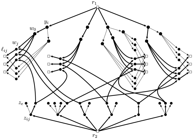
Figure 4: The constructed graph in the reduction of Section 5.3 for an instance with $k=4$, $|V_{1}|=2$, $|V_{2}|=1$, $|V_{3}|=3$, and $|V_{4}|=2$. Squares are terminals, and circles are Steiner vertices. The thick edges indicate a solution encoding a clique. For better visibility, only the edges $z_{e}w_{i}$ of the solution are shown for any edge $e$ and incident vertex $w$.

We prove that the instance to Multicoloured Clique has a clique $K$ of size $k$, if and only if there is a solution $N$ to the pure $\alpha$-diamond $H$ in $G$ with cost at most $4k^{2}-2k$. Intuitively, such a solution $N$ will determine one vertex $w$ of $K$ for each $V_{i}$, since it can only afford to include the $k$ corresponding copies $w_{j}$ when connecting $r_{1}$ to $L$ through the vertex $y_{i}$ representing $V_{i}$. At the same time $N$ will determine one edge $e$ of $K$ for each $E_{ij}$ by connecting $r_{2}$ to $L$ through one vertex $z_{e}$ for each vertex $z_{ij}$ representing $E_{ij}$. These vertices $z_{e}$ are connected to the $k-1$ copies $w_{j}$ with $j>0$ of a vertex $w\in\bigcup_{i}V_{i}$ in such a way that $e$ must be incident to $w$ in order for the paths from $r_{2}$ in $N$ to reach $L$.

Clique $\Rightarrow$ network. We first show that a solution $N$ in $G$ of cost $4k^{2}-2k$ exists if the clique $K$ exists. For every $i\in\{1,\ldots,k\}$ the solution contains the edges $r_{1}y_{i}$ and $y_{i}w_{0}$, where $w$ is the vertex of $K$ in $V_{i}$. These edges add a cost of $2k$ to $N$. We also add all edges $w_{0}w_{j}$ for the $k-1$ additional copies $w_{j}$ with $j>0$ of each vertex $w$ of $K$, which adds a cost of $k(k-1)$. For each such copy $w_{j}$ we then connect to the terminal set $L$ by adding the respective edge $w_{j}\ell_{ij}$. Note that this will add an edge incident to each terminal of $L$ to $N$ and so $r_{1}$ is connected to every terminal of $L$. At the same time the last step adds a cost of $1$ for every terminal of $L$ to $N$, which sums up to $k(k-1)$. For all $1\leq i<j\leq k$ we connect $r_{2}$ to $z_{ij}$ in the solution $N$ via the edge $r_{2}z_{ij}$ at a cost of $k\choose 2$. The clique $K$ contains one edge $e$ from every set $E_{ij}$, and we add the corresponding edges $z_{ij}z_{e}$ to $N$ at an additional cost of $k\choose 2$. For any such edge $e$ the graph $G$ contains an edge $z_{e}w_{j}$ for the incident vertex $w\in V_{i}$ and an edge $z_{e}w_{i}$ for the other incident vertex $w\in V_{j}$. We also add these respective edges to the solution at a cost of $2{k\choose 2}$. Since such an incident vertex $w\in V_{i}$ is part of the clique $K$, the respective copy $w_{j}$ is connected to the terminal $\ell_{ij}\in L$ in $N$. Moreover, every copy $w_{j}$ that is part of $N$ can be reached from the vertex $z_{e}$ in $N$ for the corresponding incident edge $e$ to $w$ in $K$. Hence $r_{2}$ is connected to every terminal of $L$ in $N$, which means that $N$ is a solution to $H$ in $G$ with a total cost of $2k+2k(k-1)+4{k\choose 2}=4k^{2}-2k$.

Network $\Rightarrow$ clique. It remains to prove that any solution $N$ to $H$ in $G$ of cost at most $4k^{2}-2k$ corresponds to a clique $K$ of size $k$ in the input instance. If a solution to the pure $\alpha$-diamond $H$ exists in $G$, then all terminals of $L$ are reachable from $r_{1}$ and from $r_{2}$ in $G$. We define the reachability set $Y_{v}$ of a vertex $v\in V(G)$ as the set of vertices reachable from $v$ by a path in $G$. For each $i\in\{1,\ldots,k\}$ the set $Y_{y_{i}}$ consists of $y_{i}$, and, for $j\in\{0,\ldots,k\}$ with $j\neq i$, each $w_{j}$ with $w\in V_{i}$ and the terminals $\ell_{ij}\in L$. In particular, the sets $Y_{y_{i}}$ are disjoint and also partition the terminal set $L$. The set $Y_{r_{1}}$ consists of $r_{1}$ and the union $\bigcup_{i}Y_{y_{i}}$. Hence in order for $r_{1}$ to be connected to every terminal of $L$ in $N$, for each $i\in\{1,\ldots,k\}$ the solution needs to include the edge $r_{1}y_{i}$ and at least one edge $y_{i}w_{0}$ for some $w\in V_{i}$. Since a terminal $\ell_{ij}$ is adjacent to the $j$-th copy $w_{j}$ of every vertex $w\in V_{i}$, for each $j\neq i$ at least one edge $w_{0}w_{j}$ (for various $w\in V_{i}$) and a corresponding edge $w_{j}\ell_{ij}$ must be included in $N$. These edges contribute a cost of $2k+2k(k-1)$ to $N$.

Now consider the reachability set $Y_{z_{ij}}$ for some $1\leq i<j\leq k$. It consists of $z_{ij}$, all $z_{e}$ with $e\in E_{ij}$, the $j$-th copy $w_{j}$ of every vertex $w\in V_{i}$ incident to edges of $E_{ij}$, the $i$-th copy $w_{i}$ of all vertices $w\in V_{j}$ incident to edges of $E_{ij}$, and corresponding terminals $\ell_{ij}$ and $\ell_{ji}$. Since all terminals of $L$ are reachable from $r_{2}$ and the sets $Y_{z_{ij}}$ are disjoint, the sets $Y_{z_{ij}}$ partition $L$. The set $Y_{r_{2}}$ consists of $r_{2}$ and the union $\bigcup_{i<j}Y_{z_{ij}}$, and so for every $1\leq i<j\leq k$ the solution $N$ must contain the edge $r_{2}z_{ij}$ and at least one edge $z_{ij}z_{e}$ for some $e\in E_{ij}$. In order for $r_{2}$ to connect to $\ell_{ij}$ in $N$, the solution must also contain the edge $z_{e}w_{j}$ for some $w\in V_{i}$ incident to $e\in E_{ij}$. Analogously, the solution must also contain the edge $z_{e}w_{i}$ for $r_{2}$ to reach $\ell_{ji}$ in $N$ for some $w\in V_{j}$ incident to some $e\in E_{ij}$. These edges contribute a cost of $4{k\choose 2}$ to $N$.

Since all these necessary edges in $N$ sum up to a cost $2k+2k(k-1)+4{k\choose 2}=4k^{2}-2k$, they are also the only edges present in $N$. In particular, for each $i\in\{1,\ldots,k\}$ the solution contains exactly one edge $y_{i}w_{0}$ for some $w\in V_{i}$, and therefore also must contain the $2(k-1)$ corresponding edges $w_{0}w_{j}$ and $w_{j}\ell_{ij}$ for $j\neq i$. On the other hand, for every $1\leq i<j\leq k$ the solution contains exactly one edge $z_{ij}z_{e}$ for some $e\in E_{ij}$, and therefore also must contain the corresponding edge $z_{e}w_{j}$ for the incident vertex $w\in V_{i}$ to $e$ and the corresponding edge $z_{e}w_{i}$ for the incident vertex $w\in V_{j}$ to $e$. Hence the solution $N$ corresponds to a subgraph of the instance of Multicoloured Clique with $k$ pairwise adjacent vertices, i.e., it is a clique $K$ of size $k$. ∎

The reduction for the case when the pattern is a flawed $\alpha$-diamond is essentially the same as the one for pure $\alpha$-diamonds, as we show next.

Lemma .

If ${\mathcal{H}}$ is the class of all flawed out-diamonds, then ${\mathcal{H}}$-DSN is W[1]-hard parameterized by the number of terminals. The same holds if ${\mathcal{H}}$ is the class of all flawed in-diamonds.

Proof.

We only describe the case when $H$ is an out-diamond, as the other case is symmetric. The reduction builds on the one given in Section 5.3: we simply add the additional terminal $x$ of $H$ to $G$, and connect it to $r_{1}$ and $r_{2}$ in $G$ by edges $xr_{1}$ and $xr_{2}$ with cost $1$ each. Given a clique of size $k$ in an instance to Multicoloured Clique, consider the network $N$ in $G$ of cost $4k^{2}-2k$ suggested in Section 5.3. We add the edges $xr_{1}$ and $xr_{2}$ to $N$, which results in a solution of cost $4k^{2}-2k+2$ for the flawed $\alpha$-diamond $H$. On the other hand, any solution to $H$ must contain a path from $x$ to $r_{1}$ and from $x$ to $r_{2}$. Since there is no path from $r_{1}$ to $r_{2}$, nor from $r_{2}$ to $r_{1}$ in the constructed graph $G$, any solution to $H$ must contain both the edge $xr_{1}$ and the edge $xr_{2}$. Thus the minimal cost solution to $H$ in $G$ has cost $4k^{2}-2k+2$ and corresponds to a clique of size $k$ in the Multicoloured Clique instance, as argued in the proof of Section 5.3. ∎

Given the three reductions above, we can now prove Theorem 5.1, based on the additional reduction given in Section 5.1.

Proof (of Theorem 5.1).

Let ${\mathcal{H}}^{\prime}$ be the closure of ${\mathcal{H}}$ under identifying vertices and transitive equivalence. By assumption, ${\mathcal{H}}$ is not in ${\mathcal{C}}^{*}_{\lambda,\delta}$ for any $\lambda$ and $\delta$, and this is also true for the superset ${\mathcal{H}}^{\prime}$ of ${\mathcal{H}}$. Thus Section 5.2 implies that ${\mathcal{H}}^{\prime}$ fully contains one of five classes: the class of all directed cycles, pure in-diamonds, pure out-diamonds, etc. Suppose for example that ${\mathcal{H}}^{\prime}$ contains the class of all directed cycles, which we will denote by ${\mathcal{H}}^{\prime\prime}$. By Section 5.3, we know that ${\mathcal{H}}^{\prime\prime}$-DSN is W[1]-hard and ${\mathcal{H}}^{\prime\prime}$ is obviously decidable. Thus we can invoke Section 5.1 to obtain that there is a parameterized reduction from ${\mathcal{H}}^{\prime\prime}$-DSN to ${\mathcal{H}}$-DSN, and hence we can conclude that the latter problem is also W[1]-hard. The proof is similar in the other cases, when ${\mathcal{H}}^{\prime}$ contains, e.g., every pure in-diamond or every flawed in-diamond: then we use Section 5.3 or Section 5.3 instead of Section 5.3. ∎

References

- [1] Ajit Agrawal, Philip N. Klein and R. Ravi “When Trees Collide: An Approximation Algorithm for the Generalized Steiner Problem on Networks” In SIAM J. Comput. 24.3, 1995, pp. 440–456 DOI: 10.1137/S0097539792236237
- [2] Aaron Archer, MohammadHossein Bateni, MohammadTaghi Hajiaghayi and Howard J. Karloff “Improved Approximation Algorithms for Prize-Collecting Steiner Tree and TSP” In SIAM J. Comput. 40.2, 2011, pp. 309–332 DOI: 10.1137/090771429
- [3] MohammadHossein Bateni, Mohammad Taghi Hajiaghayi and Dániel Marx “Approximation Schemes for Steiner Forest on Planar Graphs and Graphs of Bounded Treewidth” In J. ACM 58.5, 2011, pp. 21 DOI: 10.1145/2027216.2027219
- [4] MohammadHossein Bateni and MohammadTaghi Hajiaghayi “Euclidean Prize-Collecting Steiner Forest” In Algorithmica 62.3-4, 2012, pp. 906–929 DOI: 10.1007/s00453-011-9491-8
- [5] MohammadHossein Bateni, MohammadTaghi Hajiaghayi and Vahid Liaghat “Improved Approximation Algorithms for (Budgeted) Node-Weighted Steiner Problems” In 40th International Colloquium on Automata, Languages, and Programming, 2013, pp. 81–92 DOI: 10.1007/978-3-642-39206-1˙8
- [6] Hans L. Bodlaender “Some Classes of Graphs with Bounded Treewidth” In Bulletin of the EATCS 36, 1988, pp. 116–125
- [7] Glencora Borradaile, Philip N. Klein and Claire Mathieu “A Polynomial-Time Approximation Scheme for Euclidean Steiner Forest” In ACM Transactions on Algorithms 11.3, 2015, pp. 19:1–19:20 DOI: 10.1145/2629654
- [8] Glencora Borradaile, Philip N. Klein and Claire Mathieu “An O(n log n) approximation scheme for Steiner tree in planar graphs” In ACM Transactions on Algorithms 5.3, 2009 DOI: 10.1145/1541885.1541892
- [9] Jaroslaw Byrka, Fabrizio Grandoni, Thomas Rothvoß and Laura Sanità “Steiner Tree Approximation via Iterative Randomized Rounding” In J. ACM 60.1, 2013, pp. 6 DOI: 10.1145/2432622.2432628
- [10] Moses Charikar, Chandra Chekuri, To-Yat Cheung, Zuo Dai, Ashish Goel, Sudipto Guha and Ming Li “Approximation Algorithms for Directed Steiner Problems” In J. Algorithms 33.1, 1999, pp. 73–91 DOI: 10.1006/jagm.1999.1042
- [11] Chandra Chekuri, Guy Even, Anupam Gupta and Danny Segev “Set connectivity problems in undirected graphs and the directed steiner network problem” In ACM Transactions on Algorithms 7.2, 2011, pp. 18 DOI: 10.1145/1921659.1921664
- [12] Chandra Chekuri, Mohammad Taghi Hajiaghayi, Guy Kortsarz and Mohammad R. Salavatipour “Approximation algorithms for node-weighted buy-at-bulk network design” In Proceedings of the Eighteenth Annual ACM-SIAM Symposium on Discrete Algorithms, 2007, pp. 1265–1274 URL: http://dl.acm.org/citation.cfm?id=1283383.1283519
- [13] Rajesh Chitnis, Andreas Emil Feldmann and Pasin Manurangsi “Parameterized Approximation Algorithms for Bidirected Steiner Network Problems” In 26th Annual European Symposium on Algorithms, ESA, 2018, pp. 20:1–20:16
- [14] Rajesh Hemant Chitnis, Hossein Esfandiari, MohammadTaghi Hajiaghayi, Rohit Khandekar, Guy Kortsarz and Saeed Seddighin “A Tight Algorithm for Strongly Connected Steiner Subgraph on Two Terminals with Demands (Extended Abstract)” In 9th International Symposium on Parameterized and Exact Computation, 2014, pp. 159–171 DOI: 10.1007/978-3-319-13524-3˙14
- [15] Rajesh Hemant Chitnis, Andreas Emil Feldmann, Mohammad Taghi Hajiaghayi and Dániel Marx “Tight Bounds for Planar Strongly Connected Steiner Subgraph with Fixed Number of Terminals (and Extensions)” In SIAM J. Comput. 49.2, 2020, pp. 318–364 DOI: 10.1137/18M122371X
- [16] M. Cygan, F.. Fomin, L. Kowalik, D. Lokshtanov, D. Marx, M. Pilipczuk, M. Pilipczuk and S. Saurabh “Parameterized Algorithms” Springer, 2015
- [17] Erik D. Demaine, Mohammad Taghi Hajiaghayi and Philip N. Klein “Node-Weighted Steiner Tree and Group Steiner Tree in Planar Graphs” In ACM Transactions on Algorithms 10.3, 2014, pp. 13:1–13:20 DOI: 10.1145/2601070
- [18] Reinhard Diestel “Graph theory” 173, Graduate Texts in Mathematics Springer-Verlag, Berlin, 2005, pp. xvi+411
- [19] R.. Downey and M.. Fellows “Fundamentals of parameterized complexity” Springer, 2013
- [20] S.. Dreyfus and R.. Wagner “The Steiner problem in graphs” In Networks 1.3, 1971, pp. 195–207 DOI: 10.1002/net.3230010302
- [21] Eduard Eiben, Dusan Knop, Fahad Panolan and Ondrej Suchý “Complexity of the Steiner Network Problem with Respect to the Number of Terminals” In STACS, 2019, pp. 25:1–25:17
- [22] Jon Feldman and Matthias Ruhl “The Directed Steiner Network Problem is Tractable for a Constant Number of Terminals” In SIAM J. Comput. 36.2, 2006, pp. 543–561
- [23] Andreas Emil Feldmann and Dániel Marx “The Complexity Landscape of Fixed-Parameter Directed Steiner Network Problems” In 43rd International Colloquium on Automata, Languages, and Programming, (ICALP), 2016, pp. 27:1–27:14 DOI: 10.4230/LIPIcs.ICALP.2016.27
- [24] Michael R. Fellows, Danny Hermelin, Frances A. Rosamond and Stéphane Vialette “On the parameterized complexity of multiple-interval graph problems” In Theor. Comput. Sci. 410.1, 2009, pp. 53–61 DOI: 10.1016/j.tcs.2008.09.065
- [25] Jörg Flum and Martin Grohe “Parameterized complexity theory” Springer, 2006
- [26] Bernhard Fuchs, Walter Kern, D Molle, Stefan Richter, Peter Rossmanith and Xinhui Wang “Dynamic programming for minimum Steiner trees” In Theory of Computing Systems 41.3 Springer, 2007, pp. 493–500
- [27] Martin Grohe and Dániel Marx “On tree width, bramble size, and expansion” In J. Comb. Theory, Ser. B 99.1, 2009, pp. 218–228 DOI: 10.1016/j.jctb.2008.06.004
- [28] Jiong Guo, Rolf Niedermeier and Ondrej Suchý “Parameterized Complexity of Arc-Weighted Directed Steiner Problems” In SIAM J. Discrete Math. 25.2, 2011, pp. 583–599 DOI: 10.1137/100794560
- [29] Richard M. Karp “Reducibility among combinatorial problems” In Complexity of computer computations Plenum, 1972, pp. 85–103
- [30] Philip N. Klein and R. Ravi “A Nearly Best-Possible Approximation Algorithm for Node-Weighted Steiner Trees” In J. Algorithms 19.1, 1995, pp. 104–115 DOI: 10.1006/jagm.1995.1029
- [31] Jesper Nederlof “Fast Polynomial-Space Algorithms Using Inclusion-Exclusion” In Algorithmica 65.4, 2013, pp. 868–884
- [32] Sridhar Rajagopalan and Vijay V. Vazirani “On the Bidirected Cut Relaxation for the Metric Steiner Tree Problem” In Proceedings of the Tenth Annual ACM-SIAM Symposium on Discrete Algorithms, 1999, pp. 742–751 URL: http://dl.acm.org/citation.cfm?id=314500.314909
- [33] Gabriel Robins and Alexander Zelikovsky “Tighter Bounds for Graph Steiner Tree Approximation” In SIAM J. Discrete Math. 19.1, 2005, pp. 122–134 DOI: 10.1137/S0895480101393155
- [34] Ondřej Suchý “On directed steiner trees with multiple roots” In International Workshop on Graph-Theoretic Concepts in Computer Science (WG), 2016, pp. 257–268
- [35] Alexander Zelikovsky “A Series of Approximation Algorithms for the Acyclic Directed Steiner Tree Problem” In Algorithmica 18.1, 1997, pp. 99–110 DOI: 10.1007/BF02523690