July 2017

In this paper, the flavor structure of quark and lepton EDMs in the SM and beyond is investigated using tools inspired from Minimal Flavor Violation. While Jarlskog-like flavor invariants are adequate for estimating $\mathcal{CP}$-violation from closed fermion loops, non-invariant structures arise from rainbow-like processes. Our goal is to systematically construct these latter flavor structures in the quark and lepton sectors, assuming different mechanisms for generating neutrino masses. Numerically, they are found typically much larger, and not necessarily correlated with, Jarlskog-like invariants. Finally, the formalism is adapted to deal with a third class of flavor structures, sensitive to the flavored $U(1)$ phases, and used to study the impact of the strong $\mathcal{CP}$-violating interaction and the interplay between the neutrino Majorana phases and possible baryon and/or lepton number violating interactions.

1 Introduction

In the Standard Model, there are two sources of $\mathcal{CP}$-violation. The first is intimately entangled with flavor physics. It comes from the quark Yukawa couplings and is encoded in the CKM matrix. It requires some -real or virtual- flavor transitions to be felt in observables, and has been extensively studied experimentally in $K$ and $B$ meson decays and mixings. The second source is more peculiar. It can be encoded in the quark Yukawa couplings also, but is intrinsically flavor blind, and receives a contribution from the QCD dynamics. It should lead to large flavor-diagonal $\mathcal{CP}$-violation effects, like a neutron electric dipole moment, but this is not confirmed experimentally, raising one of the most serious puzzles of the SM.

These two types of $\mathcal{CP}$ violating phases can be generalized beyond the SM. The first type is flavored, and comes from the way the quarks and leptons acquire their masses. In a supersymmetric context, squark and slepton masses would also bring phases of this type. Whenever Minimal Flavor Violation[1] is imposed, the impact of such flavored new phases on observables is rather limited, even if the scale of the new physics is at around the TeV. The second type of phases is flavor blind, and can originate from some extended scalar sector if some parameters are complex there, or from the non-perturbative gauge dynamics. In a supersymmetric context, gaugino masses also generate phases of this type. Being problematic already in the SM, these phases pose a challenge for any model as long as no specific dynamics is called in to explicitly tame them.

In the present paper, our goal is to investigate the impact of flavored phases on flavor-blind observables like quark and lepton EDM. Specifically, if we parametrize the magnetic operators as

$$\mathcal{L}_{eff}=e\frac{c_{u}}{\Lambda^{2}}(\bar{U}\mathbf{Y}_{u}\mathbf{X}_{u}\sigma_{\mu\nu}Q)H^{\dagger}F^{\mu\nu}+e\frac{c_{d}}{\Lambda^{2}}(\bar{D}\mathbf{Y}_{d}\mathbf{X}_{d}\sigma_{\mu\nu}Q)H^{\dagger}F^{\mu\nu}+e\frac{c_{e}}{\Lambda^{2}}(\bar{E}\mathbf{Y}_{e}\mathbf{X}_{e}\sigma_{\mu\nu}L)H^{\dagger}F^{\mu\nu}+...\;,$$ (1)

where $Q,L,U,D,E$ are the quark and lepton weak doublets, up-quark, down-quark, and lepton weak singlets, respectively, our goal is to study the phases coming from the flavor structures $\mathbf{Y}_{u,d,e}\mathbf{X}_{u,d,e}$, which are three-by-three matrices in flavor space. This includes all the flavored phases, plus those flavor-blind phases originating from the quark and lepton couplings to Higgs boson(s), or more generally those can be absorbed into these couplings, like the strong $\mathcal{CP}$-violating phase in the quark sector or the overall Majorana phase in the lepton sector. On the contrary, the flavor-blind phases not related to quark or lepton couplings are necessarily encoded in the Wilson coefficients $c_{u,d,e}$, and will thus be taken real here.

In the SM, $\mathbf{X}_{u,d,e}$ are polynomials in $\mathbf{Y}_{u,d,e}$, since those are the only available flavor structures. In the spirit of Minimal Flavor Violation[1], which is exact in the SM, the form of these polynomials can be derived straightforwardly using the flavor symmetry, and treating the Yukawa couplings as symmetry-breaking spurions. It is then well-known that $\operatorname{Im}\mathbf{X}_{e}^{11}$ tuning the electron EDM will be proportional to the Jarlskog determinant $\det[\mathbf{Y}_{u}^{\dagger}\mathbf{Y}_{u},\mathbf{Y}_{d}^{\dagger}\mathbf{Y}_{d}]$. This is the only $\mathcal{CP}$-violating flavor invariant that can be constructed in the SM [2]. It is not a reliable measure of $\mathcal{CP}$ violation though, since $\operatorname{Im}\mathbf{X}_{d}^{11}$ tuning the down quark EDM is larger by no less than 10 orders of magnitude. It is not proportional to the Jarlskog determinant, but rather to $\mathbf{X}_{d}=\mathbf{[Y}_{u}^{\dagger}\mathbf{Y}_{u}\;,\;\mathbf{Y}_{u}^{\dagger}\mathbf{Y}_{u}\mathbf{Y}_{d}^{\dagger}\mathbf{Y}_{d}\mathbf{Y}_{u}^{\dagger}\mathbf{Y}_{u}]$. The derivation of this commutator from the flavor symmetry and its properties will be explored in Section 3.

Let us stress that this commutator structure is not new by itself [3]. Actually, even exact computations of the quark EDM have been performed [4, 5]. However, its derivation alongside $\mathcal{CP}$-violating invariant using only the flavor symmetry has not been presented before. Further, this serves us as a warming-up for Section 4, where neutrino mass terms are introduced. The neutrino flavor structures open new ways to generate imaginary parts for $\mathbf{X}_{u,d,e}$. Here again, flavor invariants have been extensively studied (see in particular Ref. [6] and references there), but the systematic analysis of the corresponding non-invariant commutators has not. As for the CKM contributions to the quark and lepton EDMs, we will find that the invariants are not adequate to estimate the order of magnitude of the lepton EDM, because the non-invariant commutators are in general much larger.

Before entering the core of the discussion, we start by reviewing briefly in the next Section the flavor symmetry techniques used throughout this paper, taking the quark FCNC as examples (this section is partly based on Ref. [7]). Then, the CKM contribution to the EDM is analyzed in Section 3. We also show how to extend the formalism to deal with the strong $\mathcal{CP}$ term, and estimate the induced quark and lepton EDMs. In Section 4, neutrino masses are turned on. The invariant and non-invariant flavor structures tuning the quark and lepton EDMs are constructed separately for the Dirac mass case, Majorana mass case, and the three simplest seesaw mechanisms. We also look at peculiar lepton-number violating invariants that could arise in the Majorana case, and estimate their possible impact on EDMs. Finally, we conclude in Section 5, and collect the Cayley-Hamilton identities needed in the text in Appendix A.

2 How to exploit the SM flavor symmetry?

The gauge sector of the SM is invariant under a large global symmetry group [8]

$$G_{F}=U(3)^{5}=U(3)_{Q}\otimes U(3)_{U}\otimes U(3)_{D}\otimes U(3)_{L}\otimes U(3)_{E}\;,$$ (2)

which is called the flavor symmetry. The action of this group is defined such that left-handed doublets and right-handed singlets transform as $\mathbf{3}$ under their respective $U(3)$, i.e., $X\rightarrow g_{X}X$, $g_{X}\in U(3)_{X}$ for $X=Q,L,U,D,E$. This symmetry is not exact in the SM though. It is explicitly broken by the couplings of fermions with the Higgs field,

$$\mathcal{L}_{\text{Yukawa}}=-\bar{U}\mathbf{Y}_{u}QH^{\dagger C}-\bar{D}\mathbf{Y}_{d}QH^{\dagger}-\bar{E}\mathbf{Y}_{e}LH^{\dagger}+h.c.\;.$$ (3)

Clearly, the Yukawa couplings break $G_{F}$ since they mix different species of fermions.

To set the stage for the latter discussion on EDMs, the goal of this section is to show how the flavor symmetry $G_{F}$ can be used to immediately establish and understand the flavor structure of the flavor changing neutral currents (FCNC). As a first step, the flavor symmetry is formally restored by promoting the Yukawa couplings to spurions, i.e., static fields with the definite transformation properties

$$\mathbf{Y}_{u} \sim\left(\mathbf{\bar{3}},\mathbf{3},\mathbf{1},\mathbf{1},\mathbf{1}\right)_{G_{F}}:\mathbf{Y}_{u}\overset{G_{F}}{\rightarrow}g_{U}\mathbf{Y}_{u}g_{Q}^{\dagger}\;,\;$$ (4a)

$$\mathbf{Y}_{d} \sim\left(\mathbf{\bar{3}},\mathbf{1},\mathbf{3},\mathbf{1},\mathbf{1}\right)_{G_{F}}:\mathbf{Y}_{d}\overset{G_{F}}{\rightarrow}g_{D}\mathbf{Y}_{d}g_{Q}^{\dagger}\;,$$ (4b)

$$\mathbf{Y}_{e} \sim\left(\mathbf{1},\mathbf{1},\mathbf{1},\mathbf{\bar{3}},\mathbf{3}\right)_{G_{F}}:\mathbf{Y}_{e}\overset{G_{F}}{\rightarrow}g_{E}\mathbf{Y}_{e}g_{L}^{\dagger}\;.$$ (4c)

This is a purely formal but extremely fruitful manipulation. Once the SM Lagrangian becomes invariant under $$G_{F} G_{F}$$, even if artificially, the SM amplitude for any possible process must also be manifestly -invariant. Crucially, this invariance may require inserting Yukawa spurions in a very specific way in the amplitude. Its flavor structure can thus be established quite precisely without embarking into any computation. This even translates into quantitative predictions once the spurions are frozen back to their physical values. To identify them, consider the Yukawa couplings after the electroweak Spontaneous Symmetry Breaking (SSB),

$$\mathcal{L}_{\text{Yukawa}}=-v\left(\bar{u}_{R}\mathbf{Y}_{u}u_{L}+\bar{d}_{R}\mathbf{Y}_{d}d_{L}+\bar{e}_{R}\mathbf{Y}_{e}e_{L}\right)\left(1+\frac{h}{v}\right)+h.c.\;.$$ (5)

A priori, none of these couplings is diagonal in flavor space. Their singular value decomposition (SVD) are denoted as

$$vV_{R}^{u,d,e}\mathbf{Y}_{u,d,e}V_{L}^{u,d,e}=\mathbf{m}_{u,d,e}\;,$$ (6)

where the mass matrices $\mathbf{m}_{u,d,e}$ are diagonal. So, a gauge-invariant $G_{F}$ transformation with $g_{U,D,E}=V_{R}^{u,d,e}$, $g_{L}=V_{L}^{e}$, and for example $g_{Q}=V_{L}^{d}$ leads to

$$v\mathbf{Y}_{u}\overset{frozen}{\rightarrow}\mathbf{m}_{u}V_{CKM},\;\;v\mathbf{Y}_{d}\overset{frozen}{\rightarrow}\mathbf{m}_{d},\;\;v\mathbf{Y}_{e}\overset{frozen}{\rightarrow}\mathbf{m}_{e}\;,$$ (7)

with $V_{CKM}\equiv V_{L}^{u}V_{L}^{d\dagger}$. These are the physical values of the spurions in the gauge-basis in which all but the $u_{L}$ quarks are mass eigenstates (that with all but $d_{L}$ quarks would move the $V_{CKM}$ factor into $\mathbf{Y}_{d}$). In this way, some processes are immediately predicted to be very suppressed compared to others as a result of the very peculiar numerical hierarchies of $\mathbf{m}_{u,d,e}$ and $V_{CKM}$. Also, it is immediate to see that no leptonic FCNC are allowed since after inserting $\mathbf{Y}_{e}$ in an amplitude with external lepton fields, it gets frozen to its diagonal background $\mathbf{m}_{e}/v$.

Let us see in practice how this technique works. To be able to use the $G_{F}$ symmetry of the gauge sector, it better not be spontaneously broken yet. All renormalizable dimension-four couplings are already part of the SM Lagrangian and do not induce FCNC. Turning to dimension-six operators, we consider the following four illustrative examples:

$$\mathcal{L}_{\text{eff}}=\frac{a_{1}}{\Lambda^{2}}(\bar{Q}\gamma_{\nu}Q)D_{\mu}F^{\mu\nu}+\frac{a_{2}}{\Lambda^{2}}(\bar{D}\gamma_{\nu}D)D_{\mu}F^{\mu\nu}+\frac{a_{3}}{\Lambda^{2}}(\bar{Q}\gamma_{\mu}Q)H^{\dagger}D^{\mu}H+\frac{a_{4}}{\Lambda^{2}}(\bar{D}\sigma_{\mu\nu}Q)H^{\dagger}F^{\mu\nu}+...$$ (8)

All these operators are generated in the SM at the loop level, see Fig. 1, so we set $\Lambda^{2}\sim M_{W}^{2}/g^{2}\sim G_{F}^{-1}$. The Wilson coefficients are to be understood as $3\times 3$ matrices in flavor space, with for example $a_{1}\bar{Q}\gamma_{\nu}Q\equiv a_{1}^{IJ}\bar{Q}^{I}\gamma_{\nu}Q^{J}$. As at the fundamental level, the only flavored couplings are the Yukawa couplings, these Wilson coefficients are functions of $\mathbf{Y}_{u,d}$. Assuming polynomial expressions, the $G_{F}$ symmetry imposes the structures

$$a_{1},a_{3} =\mathbf{1}\oplus\mathbf{Y}_{d}^{\dagger}\mathbf{Y}_{d}\oplus\mathbf{Y}_{u}^{\dagger}\mathbf{Y}_{u}\oplus...\;,$$ (9a)

$$a_{2} =\mathbf{1\oplus Y}_{d}\mathbf{Y}_{d}^{\dagger}\oplus\mathbf{Y}_{d}\mathbf{Y}_{u}^{\dagger}\mathbf{Y}_{u}\mathbf{Y}_{d}^{\dagger}\oplus...\;,$$ (9b)

$$a_{4} =\mathbf{Y}_{d}(\mathbf{1}\oplus\mathbf{Y}_{d}^{\dagger}\mathbf{Y}_{d}\oplus\mathbf{Y}_{u}^{\dagger}\mathbf{Y}_{u}\oplus...)\;,$$ (9c)

where the $$\oplus \mathcal{O}(1) \mathbf{Y}_{u}^{\dagger}\mathbf{Y}_{u} v^{2}\mathbf{Y}_{u}^{\dagger}\mathbf{Y}_{u}\rightarrow m^{2}\mathbf{1} \mathbf{m}_{u}\rightarrow m\mathbf{1} \mathbf{Y}_{u}^{\dagger}\mathbf{Y}_{u}$$’s serve as reminders that different numbers may appear as coefficients for each term of these expansions. Once the spurions have been appropriately introduced, they are frozen to their physical values in some gauge basis. When transitions between on-shell down-type quarks are considered, the values of Eq. (7) are appropriate, and the non-diagonal structure emerges as the leading one able to induce flavor transitions. It correctly account for the GIM mechanism [9] since the unitarity of the CKM matrix ensures when . So, embodies a quadratic breaking of the GIM mechanism:

$$v^{2}(\mathbf{Y}_{u}^{\dagger}\mathbf{Y}_{u})^{IJ}=\sum_{q=u,c,t}m_{q}^{2}V_{qd^{I}}^{\ast}V_{qd^{J}}\approx m_{t}^{2}V_{td^{I}}^{\ast}V_{td^{J}}\;,$$ (10)

and the Wilson coefficients are predicted as

$$a_{1,3}^{I\neq J} \rightarrow\alpha_{1,2}\frac{m_{t}^{2}}{v^{2}}V_{tI}^{\dagger}V_{tJ}\;,$$ (11a)

$$a_{2}^{I\neq J} \rightarrow\alpha_{3}\frac{m_{d^{I}}m_{d^{J}}}{v^{2}}\frac{m_{t}^{2}}{v^{2}}V_{tI}^{\dagger}V_{tJ}\;,$$ (11b)

$$a_{4}^{I\neq J} \rightarrow\alpha_{4}\frac{m_{d^{I}}}{v}\frac{m_{t}^{2}}{v^{2}}V_{tI}^{\dagger}V_{tJ}\;,$$ (11c)

with $$\alpha_{i} \mathcal{O}(1) W a_{2}\ll a_{1} m_{d,s,b}\ll v$$ some real numbers at most of . This shows that using only the flavor symmetry, we are able to correctly predict not only the CKM scaling of the FCNC transitions, but also the chirality flips. In the above case, the operators involving right-handed quarks requires some flips because the boson couples only to left-handed fermions. This means in particular that since , and the corresponding operator can be neglected.

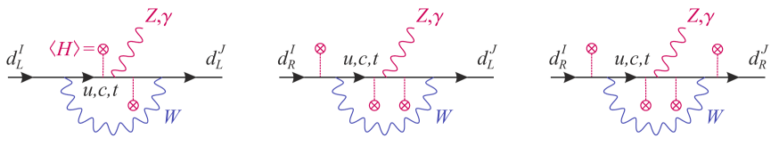
Figure 1: The $Z$ and $\gamma$ penguin diagrams contributing to the FCNC operator in Eq. (8). Yukawa insertions, depicted by the crossed tadpoles, bring in the necessary flavor-symmetry breaking, see Eq. (9).

Putting things together, the virtual photon penguin amplitude induced by the $(\bar{Q}\gamma_{\nu}Q)D_{\mu}F^{\mu\nu}$ operator is:

$$\mathcal{M}\left(\bar{d}^{I}d^{J}\rightarrow\gamma^{\ast}\left(q\right)\right)\sim\alpha_{1}\times G_{F}\times\frac{e}{4\pi^{2}}\times\bar{d}_{L}^{I}\gamma_{\mu}d_{L}^{J}\times(q^{\mu}q^{\nu}-q^{2}g^{\mu\nu})\times A_{\nu}\times\sum_{q}\frac{m_{q}^{2}}{v^{2}}V_{qd^{I}}^{\ast}V_{qd^{J}}\;.$$ (12)

The $Z$-boson penguin amplitude corresponds to the $(\bar{Q}\gamma_{\mu}Q)H^{\dagger}D^{\mu}H$ operator, and is

$$\mathcal{M}\left(\bar{d}^{I}d^{J}\rightarrow Z\left(q\right)\right)\sim\alpha_{3}\times G_{F}\times\frac{e}{4\pi^{2}\sin\theta_{W}}\times\bar{d}_{L}^{I}\gamma_{\mu}d_{L}^{J}\times v^{2}\times Z^{\mu}\times\sum_{q}\frac{m_{q}^{2}}{v^{2}}V_{qd^{I}}^{\ast}V_{qd^{J}}\;.$$ (13)

The $v^{2}$-enhancement compared to the photon penguin originates from $H^{\dagger}D^{\mu}H\overset{\text{SSB}}{\rightarrow}iv^{2}(g/2\cos\theta_{W})Z^{\mu}$. It arises because the $Z$-boson Ward identity is broken, so the $q^{\mu}q^{\nu}-q^{2}g^{\mu\nu}$ projector can be traded for the $SU(2)_{L}$-breaking parameter. Finally, the last operator is called the magnetic photon penguin, and will play a special role throughout this paper. After SSB, the amplitude is

$$\mathcal{M}\left(\bar{d}^{I}d^{J}\rightarrow\gamma\left(q\right)\right)\sim\alpha_{4}\times G_{F}\times\frac{e}{4\pi^{2}}\times m_{d^{I}}\times\bar{d}_{R}^{I}\sigma_{\mu\nu}d_{L}^{J}\times F^{\mu\nu}\times\sum_{q}\frac{m_{q}^{2}}{v^{2}}V_{qd^{I}}^{\ast}V_{qd^{J}}\;.$$ (14)

It is interesting to compare these simple predictions using only the flavor symmetry to the exact SM loop computations (see e.g. Ref. [10] for a review). Apart for some inessential numerical factors, the main difference is in the GIM breaking terms, where the simple quadratic breaking is replaced by a process-dependent loop function:

$$\sum_{q}\frac{m_{q}^{2}}{v^{2}}V_{qd^{I}}^{\ast}V_{qd^{J}}\rightarrow\sum_{q}V_{qd^{I}}^{\ast}V_{qd^{J}}F(m_{q}^{2}/M_{W}^{2})\;.$$ (15)

The function $F(m_{q}^{2}/M_{W}^{2})$ produces a quardratic GIM breaking for the $Z$ penguin, but not for the photon penguins [11]. In particular, $\bar{d}^{I}d^{J}\rightarrow\gamma^{\ast}\left(q\right)$ is only logarithmic, behaving as $\log m_{q}/M_{W}$ in both the $m_{q}\rightarrow 0$ and $m_{q}\rightarrow\infty$ limits. This difference is expected when using $G_{F}$ only. Indeed, we are forced to work in the $SU(2)_{L}\otimes U(1)_{Y}$ invariant phase of the SM where fermions are massless. Spurion insertions are understood as Higgs tadpole insertions and collapse to mass insertions only after the SSB. Though this is fine to predict the flavor structure, some dynamical effects are lost in such a perturbative treatment of the fermion masses. In particular, when the massless amplitude is not safe in the infrared, the quadratic GIM breaking softens into a logarithmic breaking only. For our purpose, this is of no consequence, but it must be kept in mind.

3 How to predict the EDM generated by the CKM phase?

The flavor-symmetry formalism can also be used for flavor-conserving observables. For instance, consider the flavor-diagonal magnetic operators of Eq. (1). After the electroweak symmetry breaking, their general structure is (remember $2\sigma^{\mu\nu}\gamma_{5}=i\varepsilon^{\mu\nu\alpha\beta}\sigma_{\alpha\beta}$ and $\varepsilon^{\mu\nu\alpha\beta}F_{\alpha\beta}\equiv 2\tilde{F}^{\mu\nu}$)

$$\mathcal{H}_{eff} =c\,\bar{\psi}_{L}\sigma^{\mu\nu}\psi_{R}F_{\mu\nu}+c^{\ast}\,\bar{\psi}_{R}\sigma^{\mu\nu}\psi_{L}F_{\mu\nu}$$

$$=\left(\operatorname{Re}c\right)\bar{\psi}\sigma^{\mu\nu}\psi F_{\mu\nu}+i\left(\operatorname{Im}c\right)\bar{\psi}\sigma^{\mu\nu}\gamma_{5}\psi F_{\mu\nu}\equiv e\frac{a}{4m}\bar{\psi}\sigma^{\mu\nu}\psi F_{\mu\nu}+i\frac{d}{2}\bar{\psi}\sigma^{\mu\nu}\gamma_{5}\psi F_{\mu\nu}\;,$$ (16)

which defines the $\mathcal{CP}$-violating electric dipole moment $d$ (EDM) and the $\mathcal{CP}$-conserving magnetic anomalous moments $a=(g-2)/2$ of the particle $\psi$ (for recent reviews, see e.g. Ref. [12, 13, 14]). Using the flavor-symmetry formalism, besides the fact that $d_{\psi}\sim m_{\psi}$ and $a\sim m_{\psi}^{2}$ from the left-right structure of the magnetic operators of Eq. (1), we can also predict the (weak) order at which the CKM phase generates a quark or lepton EDM in the SM, as we now describe in details.

3.1 Lepton EDM from the SM weak phase

Let us start with the lepton EDMs, derived from the effective operator $E\mathbf{Y}_{e}\mathbf{X}_{e}\sigma_{\mu\nu}LH^{\dagger}F^{\mu\nu}$ in Eq. (1) with $\mathbf{X}_{e}$ some chains of spurion insertions and $\Lambda\approx M_{W}$ in the SM. Since $\mathbf{Y}_{e}$ has a real background value, $\mathbf{X}_{e}$ must involve $\mathbf{Y}_{u}$ and $\mathbf{Y}_{d}$, and the invariance under $G_{F}$ forces it to be the identity matrix times the trace of a chain of $\mathbf{Y}_{u}^{\dagger}\mathbf{Y}_{u}$ and $\mathbf{Y}_{d}^{\dagger}\mathbf{Y}_{d}$ factors. As those factors are hermitian, the simplest complex trace contains no less than twelve Yukawa insertions

$$\mathbf{X}_{e} =\mathbf{1}\langle(\mathbf{Y}_{d}^{\dagger}\mathbf{Y}_{d}\mathbf{)}^{2}\mathbf{Y}_{u}^{\dagger}\mathbf{Y}_{u}\mathbf{Y}_{d}^{\dagger}\mathbf{Y}_{d}(\mathbf{Y}_{u}^{\dagger}\mathbf{Y}_{u})^{2}-(\mathbf{Y}_{u}^{\dagger}\mathbf{Y}_{u})^{2}\mathbf{Y}_{d}^{\dagger}\mathbf{Y}_{d}\mathbf{Y}_{u}^{\dagger}\mathbf{Y}_{u}(\mathbf{Y}_{d}^{\dagger}\mathbf{Y}_{d}\mathbf{)}^{2}\rangle$$

$$=2i\mathbf{1}\operatorname{Im}\langle(\mathbf{Y}_{d}^{\dagger}\mathbf{Y}_{d}\mathbf{)}^{2}\mathbf{Y}_{u}^{\dagger}\mathbf{Y}_{u}\mathbf{Y}_{d}^{\dagger}\mathbf{Y}_{d}(\mathbf{Y}_{u}^{\dagger}\mathbf{Y}_{u})^{2}\rangle=\mathbf{1}\det[\mathbf{Y}_{u}^{\dagger}\mathbf{Y}_{u},\mathbf{Y}_{d}^{\dagger}\mathbf{Y}_{d}]\equiv 2i\mathbf{1}J_{\mathcal{CP}}\;.$$ (17)

Note that the minus sign in the first term is necessary to avoid reduction towards simpler structures using Cayley-Hamilton (CH) identities [15], see Appendix A. The last equality also follows from the CH theorem. This quantity actually reduces to the very suppressed Jarlskog invariant [2]:

$$J_{\mathcal{CP}}=\mathcal{J}_{\mathcal{CP}}\times\prod_{\begin{subarray}{c}i>j=d,s,b\\ i>j=u,c,t\end{subarray}}\frac{m_{i}^{2}-m_{j}^{2}}{v^{2}}\approx\mathcal{J}_{\mathcal{CP}}\times\frac{m_{b}^{4}m_{s}^{2}m_{c}^{2}}{v^{8}}\approx 10^{-22}\;,$$ (18)

where in the standard CKM parametrization [16]

$$\mathcal{J}_{\mathcal{CP}}=\frac{1}{4}\sin(2\theta_{12})\sin(2\theta_{23})\cos^{2}(\theta_{13})\sin(\theta_{13})\sin(\delta_{13})\approx 3\times 10^{-5}\;.$$ (19)

Note that $J_{\mathcal{CP}}$ vanishes if any two up or down-type quarks are degenerate, in a way reminiscent to the freedom one would get in that case to rotate the $\mathcal{CP}$-violating phase away.

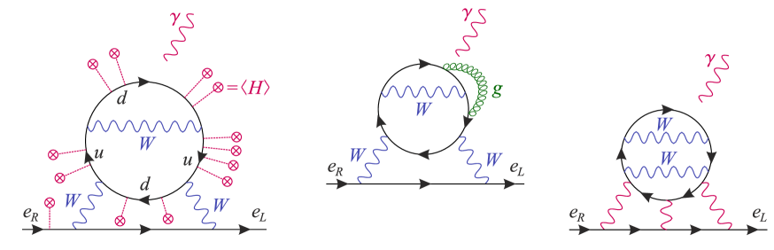
Figure 2: The CKM-induced EDM of leptons in the SM. The three-loop electroweak contribution actually vanishes because the symmetry of the loop function is incompatible with the antisymmetry of the Jarlskog invariant, and either QCD or QED corrections are required to induce a non-zero lepton EDM.

This flavor structure tells us that the lepton EDM induced by the CKM matrix asks for at least three loops since a closed quark loop with four $W$ boson vertices is required, see Fig. 2. If we think of the $\mathbf{Y}_{u}$ and $\mathbf{Y}_{d}$ factors as mass insertions along a closed quark loop, what is not apparent in these expressions [17] is that a further QCD loop is actually needed. Indeed, the dynamics of the SM [18] is such that the loop function for the $(\mathbf{Y}_{d}^{\dagger}\mathbf{Y}_{d}\mathbf{)}^{2}\mathbf{Y}_{u}^{\dagger}\mathbf{Y}_{u}\mathbf{Y}_{d}^{\dagger}\mathbf{Y}_{d}(\mathbf{Y}_{u}^{\dagger}\mathbf{Y}_{u})^{2}$ and $(\mathbf{Y}_{d}^{\dagger}\mathbf{Y}_{d}\mathbf{)}^{2}(\mathbf{Y}_{u}^{\dagger}\mathbf{Y}_{u})^{2}\mathbf{Y}_{d}^{\dagger}\mathbf{Y}_{d}\mathbf{Y}_{u}^{\dagger}\mathbf{Y}_{u}$ insertions (see Eq. (17)) are the same. But as their sum is reducible using CH identities, $\mathcal{CP}$ is conserved and the three loop process does not contribute to the lepton EDMs. To break the symmetry of the amplitude and generate an antisymmetric combination of mass insertions, at least a further loop is required, e.g. a QCD or QED correction, see Fig. 2. We thus arrive at the rough estimate (see Ref. [19]):

$$d_{e}\sim e\frac{m_{e}}{M_{W}^{2}}\left(\frac{g^{2}}{16\pi^{2}}\right)^{3}\frac{\alpha_{S}}{4\pi}\tilde{J}_{\mathcal{CP}}\approx 10^{-48}\;e\cdot cm\;,$$ (20)

to be compared to the current limit $|d_{e}|\,<8.7\cdot 10^{-29}\;e\cdot cm\;(90\%)$ [20]. For this estimate, an enhancement factor $\tilde{J}_{\mathcal{CP}}=J_{\mathcal{CP}}$ $(v/M_{W})^{12}\approx 10^{5}$ is included. Indeed, while $J_{\mathcal{CP}}$ is defined from the Yukawa couplings, and involves ratios of quark masses to the EW vacuum expectation value $v\approx 174\,$GeV, one would rather expect ratios of the quark masses in the loop to the EW gauge boson mass in a diagrammatic approach.

The same quark loop drives the EDM of the $W$ boson (suffices to cut the two lower $W$ propagators in Fig. 2), as well as those of the heavier leptons. Up to dynamical effects related to the different scales of these processes, we thus expect the well-known relation

$$\frac{d_{e}}{m_{e}}=\frac{d_{\mu}}{m_{\mu}}=\frac{d_{\tau}}{m_{\tau}}\;,$$ (21)

to hold, and thus $d_{\mu}$ and $d_{\tau}$ to be about $200$ and $4000$ times larger than $d_{e}$. Though these estimates are not very precise, they all stand well beyond our reach experimentally, since the current limits are $|d_{\mu}|<1.9\cdot 10^{-19}\;e\cdot cm\;(95\%)$ [21] and $d_{\tau}\in[-2.2,4.5]\cdot 10^{-17}\;e\cdot cm\;(95\%)$ [22]. Those are far weaker than for $d_{e}$ which exploits the very high electric field present in the $ThO$ molecule. By contrast, the bound on $d_{\mu}$ was obtained alongside the precise $(g-2)_{\mu}$ measurement, and that for $d_{\tau}$ from the study of the $\gamma\tau^{+}\tau^{-}$ vertex using the $e^{+}e^{-}\rightarrow\tau^{+}\tau^{-}$ process at Belle.

At this stage, a word of caution about the mass dependences should be stressed. As for the photon penguin $sd\rightarrow\gamma^{\ast}$ discussed before, or the similar $sd\rightarrow g^{\ast}$ gluon penguin, the mass-insertion approximation inherent to the spurion technique is unable to catch logarithmic mass dependences. Though an explicit computation of this four-loop amplitude has not been done yet, such dependencies were found for the similar CKM-induced triple gluon $\mathcal{CP}$-violating operator, $f^{abc}\tilde{G}_{\mu\nu}^{a}G^{b,\nu\rho}G_{\rho\mu}^{c}$ [23]. In particular, heavy quark factors like the two $m_{b}^{2}/v^{2}$ suppression factors in $\mathbf{X}_{e}$ get replaced by logarithms of ratios of quark and $W$ boson masses. For this reason, up to a few orders of magnitude enhancement are understood for estimates like Eq. (20).

3.2 Quark EDM from the SM weak phase

Turning to the EDM of quarks, their generation may look simpler at first sight since quarks can directly feel the CKM phase. However, the spurion technique shows that this not so in practice. Consider the interactions $U\mathbf{Y}_{d}\mathbf{X}_{u}\sigma_{\mu\nu}QH^{\dagger}F^{\mu\nu}$ and $D\mathbf{Y}_{d}\mathbf{X}_{d}\sigma_{\mu\nu}QH^{\dagger}F^{\mu\nu}$ in Eq. (1) for some chain of spurions $\mathbf{X}_{u,d}$ and $\Lambda\approx M_{W}$. Concentrating first on the $d$ quark EDM, $d_{L}$ in $Q$ should be a mass eigenstate, so we must use the gauge basis in Eq. (7) and $\mathbf{Y}_{d}$ is diagonal. In that basis, $\mathbf{X}_{d}$ must be some chains of $\mathbf{Y}_{u}^{\dagger}\mathbf{Y}_{u}$ and $\mathbf{Y}_{d}^{\dagger}\mathbf{Y}_{d}$, and its $1$-$1$ entry needs to have a non-zero imaginary part to generate an EDM. But, with $\mathbf{Y}_{d}^{\dagger}\mathbf{Y}_{d}$ real and diagonal and $\mathbf{Y}_{u}^{\dagger}\mathbf{Y}_{u}$ hermitian in this basis, this requires again quite a long chain of spurions. The same is true for the up-quark EDM, working in the basis in which $\mathbf{Y}_{u}$ is diagonal.

To identify the simplest spurion chain, let us go back to fully generic spurion expansions. The combinations $\mathbf{X}_{u.d}$ both transform as octets under $SU(3)_{Q}$. In full generality, such octets can be parametrized as infinite series of products of powers of the hermitian matrices $\mathbf{A}_{u,d}\equiv\mathbf{Y}_{u,d}^{\dagger}\mathbf{Y}_{u,d}$ [24]

$$\mathbf{X}_{octet}=\sum_{i,j,k,...=0,1,2,...}z_{ijk...}\mathbf{A}_{u}^{i}\mathbf{A}_{d}^{j}\mathbf{A}_{u}^{k}...\;,$$ (22)

for some appropriate coefficients $z_{ijk...}$. Since our goal is to quantify the impact of the CKM phase on EDM, these $z_{ijk...}$ coefficients are taken as real. Then, this series can be partially resummed using the CH identities, which permit to express higher powers of any matrices in terms of its lower powers, traces, and determinant. For example, a term $\mathbf{A}_{u}^{3}$ can be absorbed into redefinitions of the $z$, $z_{1}$, and $z_{2}$ coefficients using Eq. (129). This leaves the octet operator $\mathbf{X}_{octet}$ with $17$ terms:

$$\mathbf{X}_{octet} =x_{1}\mathbf{1}+x_{2}\mathbf{A}_{u}+x_{3}\mathbf{A}_{d}+x_{4}\mathbf{A}_{u}^{2}+x_{5}\mathbf{A}_{d}^{2}+x_{6}\{\mathbf{A}_{u},\mathbf{A}_{d}\}+x_{7}i[\mathbf{A}_{u},\mathbf{A}_{d}]+x_{8}\mathbf{A}_{u}\mathbf{A}_{d}\mathbf{A}_{u}$$

$$\;\;\;\;+x_{9}i[\mathbf{A}_{d},\mathbf{A}_{u}^{2}]+x_{10}\mathbf{A}_{d}\mathbf{A}_{u}\mathbf{A}_{d}+x_{11}i[\mathbf{A}_{u},\mathbf{A}_{d}^{2}]+x_{12}\mathbf{A}_{d}\mathbf{A}_{u}^{2}\mathbf{A}_{d}+x_{13}i[\mathbf{A}_{u}^{2},\mathbf{A}_{d}^{2}]$$

$$\;\;\;\;+x_{14}i[\mathbf{A}_{u},\mathbf{A}_{u}\mathbf{\mathbf{A}}_{d}\mathbf{A}_{u}]+x_{15}i[\mathbf{A}_{d},\mathbf{A}_{d}\mathbf{A}_{u}\mathbf{A}_{d}]$$

$$\;\;\;\;+x_{16}i[\mathbf{A}_{u},\mathbf{A}_{u}\mathbf{\mathbf{A}}_{d}^{2}\mathbf{A}_{u}]+x_{17}i[\mathbf{A}_{d},\mathbf{A}_{d}\mathbf{\mathbf{A}}_{u}^{2}\mathbf{A}_{d}]\;.$$ (23)

The only non-trivial reduction is that for the term $\mathbf{A}_{d}^{2}\mathbf{\mathbf{A}}_{u}\mathbf{A}_{d}\mathbf{\mathbf{A}}_{u}^{2}$, which can be achieved by plugging $\mathbf{X}=[\mathbf{A}_{u},\mathbf{A}_{d}]$ in Eq. (129). Also, we have used the hermiticity of $\mathbf{A}_{u,d}$ to write $\mathbf{X}_{octet}$ entirely in terms of independent hermitian combinations of spurions [15].

Let us stress that it is crucial to use only CH identities for this reduction, and not simply a projection of $\mathbf{X}$ on a set of nine terms forming an algebraic basis for the three-by-three complex matrices. First, the CH reduction never generates large numerical coefficients because the traces satisfy $\langle\mathbf{A}_{u,d}\rangle\lesssim\mathcal{O}(1)$. Second, if the $z_{ijk...}$ are real, then the $x_{i}$ may at most develop imaginary parts proportional to the Jarlskog invariant in Eq. (17). This is important because it ensures for example that $\mathbf{X}^{11}$ is either proportional to $\mathcal{J}_{\mathcal{CP}}$, if e.g. $x_{1}=\xi_{1}+i\xi_{2}\mathcal{J}_{\mathcal{CP}}$ for some real $\xi_{1,2}\lesssim\mathcal{O}(1)$, or induced directly by a non-trivial chain of spurions.

Specifically, the simplest chains having an intrinsic imaginary part in the gauge basis Eq. (7) are those appearing with the $x_{14}$ or $x_{16}$ coefficients. Any longer intrinsically imaginary chain of spurions can be reduced to those two terms, or to $\mathcal{J}_{\mathcal{CP}}$, and will be suppressed by factors of traces like $\langle\mathbf{Y}_{d}^{\dagger}\mathbf{Y}_{d}\mathbf{\rangle}$ and $\langle\mathbf{Y}_{u}^{\dagger}\mathbf{Y}_{u}\rangle$. For the EDM of down-type quarks, the largest term is thus

$$\mathbf{X}_{d}=\mathbf{[Y}_{u}^{\dagger}\mathbf{Y}_{u}\;,\;\mathbf{Y}_{u}^{\dagger}\mathbf{Y}_{u}\mathbf{Y}_{d}^{\dagger}\mathbf{Y}_{d}\mathbf{Y}_{u}^{\dagger}\mathbf{Y}_{u}]\;.$$ (24)

It needs to be antisymmetrized in this way because the sum of the two terms is hermitian, so with only real entries on the diagonal (besides being reducible via CH identities). On the contrary, thanks to the commutator, $\mathbf{X}_{d}$ has purely imaginary entries on the diagonal, for example:

$$\mathbf{X}_{d}^{11}=-2i\mathcal{J}_{\mathcal{CP}}\times\frac{m_{b}^{2}-m_{s}^{2}}{v^{2}}\prod_{i>j=u,c,t}\frac{m_{i}^{2}-m_{j}^{2}}{v^{2}}\approx 10^{-12}\;,$$ (25)

to be compared to $J_{\mathcal{CP}}\approx 10^{-22}$ in Eq. (18). Such a dependence on the quark mass differences was already noted in Ref. [3]. It arises here simply as the simplest antihermitian spurion insertion with non-zero diagonal entries.

The prediction for $d_{u}$ is very similar: $\mathbf{X}_{u}$ is obtained from $\mathbf{X}_{d}$ by interchanging $\mathbf{Y}_{d}\leftrightarrow\mathbf{Y}_{u}$ in Eq. (24) and working in the gauge basis in which $\mathbf{Y}_{u}$ is diagonal. The $x_{15}$ and $x_{17}$ terms have similar sizes since $m_{t}\approx v$,

$$\mathbf{X}_{u}=a_{1}\mathbf{[Y}_{d}^{\dagger}\mathbf{Y}_{d}\;,\;\mathbf{Y}_{d}^{\dagger}\mathbf{Y}_{d}\mathbf{Y}_{u}^{\dagger}\mathbf{Y}_{u}\mathbf{Y}_{d}^{\dagger}\mathbf{Y}_{d}]+a_{2}\mathbf{[Y}_{d}^{\dagger}\mathbf{Y}_{d}\;,\;\mathbf{Y}_{d}^{\dagger}\mathbf{Y}_{d}(\mathbf{Y}_{u}^{\dagger}\mathbf{Y}_{u})^{2}\mathbf{Y}_{d}^{\dagger}\mathbf{Y}_{d}]\;,$$ (26)

for some real $\mathcal{O}(1)$ coefficients $a_{1,2}$, so that

$$\mathbf{X}_{u}^{11}=2i\mathcal{J}_{\mathcal{CP}}\times\left(a_{1}\frac{m_{t}^{2}-m_{c}^{2}}{v^{2}}+a_{2}\frac{m_{t}^{4}-m_{c}^{4}}{v^{4}}\right)\prod_{i>j=d,s,b}\frac{m_{i}^{2}-m_{j}^{2}}{v^{2}}\approx 10^{-17}\;.$$ (27)

Because of the additional down-type quark mass factors, this is completely negligible compared to $\mathbf{X}_{d}^{11}$.

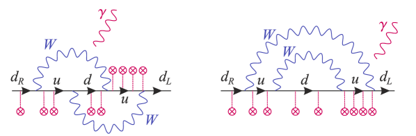
Figure 3: The electroweak rainbow diagrams leading to a down quark EDM in the SM. For each type, one example of Yukawa insertion is depicted. The final contribution requires the antisymmetrization of the insertions on the two up-type quark lines.

The electroweak rainbow diagrams behind such processes share many of the features of those generating $d_{e}$. Two $W$ boson propagators are needed (see Fig. 3), together with a further gluonic correction to break the symmetry of the loop amplitude under permutations of the mass insertions [4, 5]. The leading order thus arises at three loops, and has the generic form

$$d_{d}\sim e\frac{m_{d}}{M_{W}^{2}}\left(\frac{g^{2}}{16\pi^{2}}\right)^{2}\frac{\alpha_{S}}{4\pi}\frac{m_{b}^{2}m_{c}^{2}m_{t}^{4}}{v^{8}}\mathcal{J}_{\mathcal{CP}}\approx 10^{-36}-10^{-39}\,e\cdot cm\;,$$ (28)

depending on whether $v$ or $M_{W}$ factors appear in the denominator. Further, here also the mass-insertion approximation does not perfectly reproduce the explicit computation done in Ref. [5], where e.g. the $m_{b}^{2}$ factor turns out to soften into a logarithmic GIM breaking, enhancing the estimate by a few orders of magnitude.

One may be surprised by the non-vanishing of this expression when some down-type quarks are degenerate. To understand this, one should realize that a specific basis for these quarks is implicitly chosen by forcing the external down-type quark to be on their mass shell. If we imagine that $m_{d}=m_{s}$, then the on-shell first and second generation down quarks can be linear combinations of these. Setting

$$\left(\begin{array}[c]{c}d_{1}^{\prime}\\ d_{2}^{\prime}\end{array}\right)=\left(\begin{array}[c]{cc}\cos\theta_{ds}&\sin\theta_{ds}\\ -\sin\theta_{ds}&\cos\theta_{ds}\end{array}\right)\left(\begin{array}[c]{c}d\\ s\end{array}\right)\;,$$ (29)

so that

$$\mathbf{X}_{d}^{d_{1}d_{1}}=\cos^{2}\theta\mathbf{X}_{d}^{11}+\sin^{2}\theta\mathbf{X}_{d}^{22}+\cos\theta\sin\theta(\mathbf{X}_{d}^{12}+\mathbf{X}_{d}^{21})\;,$$ (30)

and similarly for $\mathbf{X}_{d}^{d_{2}d_{2}}$, we find that $\mathbf{X}_{d}^{d_{2}d_{2}}=\mathbf{X}_{d}^{d_{1}d_{1}}=0$ when $\theta_{ds}=\theta_{12}$ and $m_{d}=m_{s}$. This proves that $\mathcal{CP}$-conservation is recovered in the degenerate limit, as it should.

Altogether, the short-distance SM contribution to the EDM of the neutron $d_{n}\approx(4d_{d}-d_{u})/3$ is predicted to be at most one or two orders of magnitude above $10^{-36}\,e\cdot cm$. This is to be compared to the long-distance contributions which may enhance the SM contribution up $d_{n}\approx 10^{-32}\,e\cdot cm$ [27], and to the current bound which stands at $|d_{n}|<2.9\times 10^{-26}\;e\cdot cm\;(90\%)$ [28]. Note, finally, that

$$\mathbf{X}_{d}^{11}:\mathbf{X}_{d}^{22}:\mathbf{X}_{d}^{33}=m_{b}^{2}-m_{s}^{2}:m_{d}^{2}-m_{b}^{2}:m_{s}^{2}-m_{d}^{2}\;,$$ (31)

as expected from $\langle\mathbf{X}_{d}\rangle=0$. As $m_{b}\gg m_{s,d}$, this also means that $\mathbf{X}_{d}^{11}\approx\mathbf{X}_{d}^{22}\gg\mathbf{X}_{d}^{33}$. At the level of the quark EDM, these relations imply the sum rules

$$\frac{d_{d}}{m_{d}}+\frac{d_{s}}{m_{s}}+\frac{d_{b}}{m_{b}}=0\;,\;\;\frac{d_{d}}{m_{d}}\approx-\frac{d_{s}}{m_{s}}\;,\;\;\frac{d_{d}}{d_{b}}\approx\frac{m_{b}^{2}}{m_{s}^{2}}\;,$$ (32)

up to dynamical effects beyond our control. Similar relations hold for up-type quarks.

At this stage, we can now combine the information gathered for the electron and quark EDMs to obtain

$$\frac{\operatorname{Im}\mathbf{X}_{d}^{11}}{\operatorname{Im}\mathbf{X}_{e}^{11}} =\frac{-v^{4}}{(m_{b}^{2}-m_{d}^{2})(m_{s}^{2}-m_{d}^{2})}\rightarrow\left(\frac{g^{2}}{16\pi^{2}}\right)\frac{|d_{d}|}{m_{d}}\approx\frac{M_{W}^{4}}{m_{b}^{2}m_{s}^{2}}\frac{|d_{e}|}{m_{e}}\;,$$ (33)

$$\frac{\operatorname{Im}\mathbf{X}_{u}^{11}}{\operatorname{Im}\mathbf{X}_{e}^{11}} =v^{4}\frac{a_{1}+a_{2}(m_{t}^{2}+m_{c}^{2})/v^{2}}{(m_{t}^{2}-m_{u}^{2})(m_{c}^{2}-m_{u}^{2})}\rightarrow\left(\frac{g^{2}}{16\pi^{2}}\right)\frac{|d_{u}|}{m_{u}}\approx\frac{M_{W}^{2}}{m_{c}^{2}}\frac{|d_{e}|}{m_{e}}\;.$$ (34)

Numerically, we thus expect the CKM contributions to fermion EDM in the SM to scale as $|d_{d}|\approx 10^{12}\times|d_{e}|$ and $|d_{u}|\approx 10^{7}\times|d_{e}|$, up to dynamical effects.

3.3 Quark and lepton EDM from the SM strong phase

Up to now, the flavor-symmetric combinations of the spurions were required to be invariant under the full $U(3)^{5}$ symmetry. This is not consistent in the SM since three out of five combinations of these $U(1)$s are anomalous. Only the invariance under $SU(3)^{5}$ should be imposed [29]. This modifies the previous procedure in two ways. First, there are new invariants involving the Levi-Civita tensors of $SU(3)^{5}$. Given the symmetry properties of the Yukawa spurions, all these can be decomposed into $U(3)^{5}$ invariants and powers of $\det\mathbf{Y}_{u}$ and/or $\det\mathbf{Y}_{d}$. Second, the background values of the Yukawa couplings in Eq. (7) must in general include additional $\mathcal{CP}$-violating phases since the $SU(3)^{5}$ symmetry is not sufficient to make all fermion masses real.

3.3.1 Strong axial anomaly

To understand the implications for the EDMs of the quarks and leptons, let us first recall how these anomalies manifest themselves in the SM. The SVD in Eq. (6) imply the $U(1)$ transformations $3\alpha_{Q,L}=\arg\det V_{L}^{d,e\dagger}$ and $3\alpha_{U,D,E}=\arg\det V_{R}^{u,d,e}$. These phases are not fixed because the various SVD unitary matrices are defined only up to relative phases. However, these phases must satisfy

$$\arg\det\mathbf{Y}_{u}=3(\alpha_{Q}+\alpha_{U})\;,\;\arg\det\mathbf{Y}_{d}=3(\alpha_{Q}+\alpha_{D})\;,\;\arg\det\mathbf{Y}_{e}=3(\alpha_{L}+\alpha_{E})\;,$$ (35)

to make the fermion masses real. At the same time, these $U(1)$ transformations being anomalous, they induce a shift of the $G_{\mu\nu}^{a}\tilde{G}^{a,\mu\nu}$ coupling constant,

$$\theta_{C}\rightarrow\theta_{C}^{eff}=\theta_{C}-3\left(2\alpha_{Q}+\alpha_{U}+\alpha_{D}\right)=\theta_{C}-\arg\det\mathbf{Y}_{u}-\arg\det\mathbf{Y}_{d}\;,$$ (36)

where $\theta_{C}$ comes from the vacuum structure of QCD. In practice, there is thus one extra physical $\mathcal{CP}$-violating phase in the SM, $\theta_{C}^{eff}$, and one is free to account for it as a $G_{\mu\nu}^{a}\tilde{G}^{a,\mu\nu}$ coupling or as complex quark masses. Note that besides the $G_{\mu\nu}^{a}\tilde{G}^{a,\mu\nu}$ coupling, the instanton dynamics also generates the determinant interaction [30]

$$\mathcal{H}_{eff}^{axial}\sim\frac{g^{axial}}{\Lambda^{14}}(\varepsilon^{IJK}Q^{I}Q^{J}Q^{K})^{2}(\varepsilon^{IJK}U^{\dagger I}U^{\dagger J}U^{\dagger K})(\varepsilon^{IJK}D^{\dagger I}D^{\dagger J}D^{\dagger K})+h.c.\;,$$ (37)

where $Q,U,D$ here denote Weyl spinors, and the $SU(2)_{L}$, $SU(3)_{C}$, and Lorentz contractions are understood. This interaction is obviously invariant under $SU(3)^{5}$, but breaks explicitly $U(1)^{5}$ since making the quark masses real shifts the phase of this coupling to

$$g^{axial}\rightarrow g^{axial}\exp 3i(2\alpha_{Q}+\alpha_{U}+\alpha_{D})\;,$$ (38)

exactly like the strong $\theta_{C}$ in Eq. (36). Indirectly, $\arg\det\mathbf{Y}_{u}+\arg\det\mathbf{Y}_{d}$ is thus in principle accessible if $\arg(g^{axial})$ is known in some basis. The only situation in which the SM would not involve an additional free parameter is when the anomalous interactions are aligned, i.e., $\arg(g^{axial})=\theta_{C}$ before the EW symmetry breaking. In that case, making the quark masses real shifts $\theta_{C}\rightarrow\theta_{C}^{eff}$ and $\arg(g^{axial})=\theta_{C}\rightarrow\arg(g^{axial})=\theta_{C}^{eff}$.

3.3.2 Strong phase spurions and EDMs

No matter the chosen parametrization for $\theta_{C}^{eff}$, it can induce EDMs. This takes place at very low energy, through non-perturbative QCD effects. Specifically, consider the effective magnetic operators in Eq. (1), for some real $c_{u,d,e}$ and some spurion combinations $\mathbf{Y}_{u,d,e}\mathbf{X}_{u,d,e}$ sensitive to $\theta_{C}^{eff}$. As this parameter arises from QCD, and with in addition potentially large light-quarks contributions, non-local long-distance effects are dominant and $\Lambda$ should be set at the typical hadronic scale. Obviously, this pushes the effective formalism beyond its boundaries, but let us nevertheless proceed.

The main difficulty is to establish the form of the spurion insertions. Since we want to use the $G_{F}$ symmetry and its explicit breaking terms, we should move the whole $\theta_{eff}^{C}$ onto the quark masses, and get rid of the $G_{\mu\nu}^{a}\tilde{G}^{a,\mu\nu}$ coupling. This can be achieved by modifying the spurion background values to (in the gauge basis where up quarks are mass eigenstates)

$$v\mathbf{Y}_{u}\overset{frozen}{\rightarrow}e^{i\kappa\theta_{C}^{eff}\mathbf{m}_{u}^{-1}}\mathbf{m}_{u} =\mathbf{m}_{u}+i\mathbf{1}\kappa\theta_{C}^{eff}+...\;,$$ (39a)

$$v\mathbf{Y}_{d}\overset{frozen}{\rightarrow}e^{i\kappa\theta_{C}^{eff}\mathbf{m}_{d}^{-1}}\mathbf{m}_{d}V_{CKM}^{\dagger} =(\mathbf{m}_{d}+i\mathbf{1}\kappa\theta_{C}^{eff}+...\;)V_{CKM}^{\dagger}\;\;,$$ (39b)

with

$$\kappa^{-1}\equiv\langle\mathbf{m}_{u}^{-1}+\mathbf{m}_{d}^{-1}\rangle=\frac{1}{m_{u}}+\frac{1}{m_{c}}+\frac{1}{m_{t}}+\frac{1}{m_{d}}+\frac{1}{m_{s}}+\frac{1}{m_{b}}\;,$$ (40)

while we keep $v\mathbf{Y}_{e}\overset{frozen}{\rightarrow}\mathbf{m}_{e}$. Infinitely many other choices of $U(1)_{Q}\otimes U(1)_{U}\otimes U(1)_{D}$ transformations can replace the $G_{\mu\nu}^{a}\tilde{G}^{a,\mu\nu}$ coupling, but this specific choice has the following desirable properties:

• These background values correctly account for the whole of the $\theta_{C}^{eff}$ term, as can be checked by performing the anomalous rotations back to the basis $v\mathbf{Y}_{u}\rightarrow\mathbf{m}_{u}$ and $v\mathbf{Y}_{d}\rightarrow\mathbf{m}_{d}V_{CKM}^{\dagger}$,

  $$\arg\det\mathbf{Y}_{u}+\arg\det\mathbf{Y}_{d}=\arg\det\exp(i\kappa\theta_{C}^{eff}\mathbf{m}_{u}^{-1})+\arg\det\exp(i\kappa\theta_{C}^{eff}\mathbf{m}_{d}^{-1})=\theta_{C}^{eff}\;.$$ (41)

• If $g^{axial}$ is real in the basis Eq. (39), moving back to the $v\mathbf{Y}_{u}\rightarrow\mathbf{m}_{u}$ and $v\mathbf{Y}_{d}\rightarrow\mathbf{m}_{d}V_{CKM}^{\dagger}$ basis automatically aligns the phase of the instanton-induced quark transition with $G_{\mu\nu}^{a}\tilde{G}^{a,\mu\nu}$ since $g^{axial}\rightarrow g^{axial}\exp i\theta_{C}^{eff}$.

• From the basis Eq. (39), real quark masses are obtained by acting only on the right-handed fields, and the $SU(2)_{L}$ anomalous coupling $W_{\mu\nu}^{i}\tilde{W}^{i,\mu\nu}$ is not affected (this will be further discussed in the last section).

• This form ensures that both the quark and lepton EDMs induced by $\theta_{C}^{eff}$ are tuned by $\kappa$, Eq. (40), which guarantees the $\theta_{C}^{eff}$ contribution disappears whenever any of the quark mass vanishes. It also reproduces the usual factor $m_{u}m_{d}m_{s}/(m_{u}m_{d}+m_{u}m_{s}+m_{d}m_{s})$ when $m_{c,b,t}\rightarrow\infty$, and thus ensures the stability of the chiral symmetry breaking vacuum (see e.g. Ref.[31]).

• The impact of $\theta_{C}^{eff}$ is made flavor-blind even though it is introduced through the flavor couplings thanks to appropriate compensating $\mathbf{m}_{u}^{-1}$ and $\mathbf{m}_{d}^{-1}$ factors. In this respect, note that $V_{CKM}$ could be included in the exponential factor without affecting the properties of the parametrization.

To estimate the quark EDM using the $G_{F}=SU(5)^{5}$ symmetry, it suffices to set $\mathbf{X}_{u}=\mathbf{X}_{d}=\mathbf{1}$ in Eq. (1) since $\mathbf{Y}_{u,d}$ are directly sensitive to $\theta_{C}^{eff}$, so that

$$d_{u,d}\sim e\frac{1}{\Lambda_{had}^{2}}\kappa\theta_{C}^{eff}\approx\theta_{eff}\times 10^{-16}\;e\cdot cm\;,$$ (42)

for $\Lambda_{had}\approx 300$ MeV. This is very similar to naive estimates based on dimensional grounds, and implies that $\theta_{C}^{eff}\lesssim 10^{-10}$ since $|d_{n}|<2.9\times 10^{-26}\;e\cdot cm\;(90\%)$ [28]. At the level of the $SU(3)^{5}$ symmetry and its breaking terms, there is no way to gain more insight since the complicated long-distance hadronic dynamics is out of reach.

For the lepton EDM, the simplest spurion insertion is $\mathbf{X}_{e}=\mathbf{1}\det\mathbf{Y}_{u,d}$, which develops an imaginary part as

$$\operatorname{Im}\det\mathbf{Y}_{u}\rightarrow\det(\mathbf{m}_{u}/v)\operatorname{Im}\det\exp(i\kappa\theta_{C}^{eff}\mathbf{m}_{u}^{-1})\approx i\kappa\theta_{C}^{eff}\det(\mathbf{m}_{u}/v)\langle\mathbf{m}_{u}^{-1}\rangle\approx\theta_{C}^{eff}\times 10^{-7}\;.$$ (43)

A similar expression holds for $\operatorname{Im}\det\mathbf{Y}_{d}\approx\theta_{C}^{eff}\times 10^{-10}$. The quark mass factors bring in a strong suppression, but are unavoidable to consistently embed $\theta_{C}^{eff}$ in the Yukawa background values. Also, they cannot be represented as mass insertions along a closed quark loop, which are necessarily invariant under $U(5)^{5}$. So, the dependence of the closed quark loop on $\det\mathbf{Y}_{u,d}$ must rather come from the non-perturbative dressing by strong interaction effects. As this cannot be estimated here, the best we can do is derive an upper bound on the electron EDM by attaching the quark loop to the lepton current either via three photons or two weak bosons,

$$d_{e} \lesssim e\frac{m_{e}}{\Lambda_{had}^{2}}\left(\frac{e^{2}}{16\pi^{2}}\right)^{3}\operatorname{Im}\det\mathbf{Y}_{u}\approx\theta_{C}^{eff}\times 10^{-34}\;e\cdot cm\;,$$ (44)

$$d_{e} \lesssim e\frac{m_{e}}{M_{W}^{2}}\left(\frac{g^{2}}{16\pi^{2}}\right)^{2}\operatorname{Im}\det\mathbf{Y}_{u}\approx\theta_{C}^{eff}\times 10^{-32}\;e\cdot cm\;,$$ (45)

and $\Lambda_{had}\approx 300$ MeV represent the typical hadronic scale. These contributions to the lepton EDMs are certainly well beyond our reach since $\theta_{C}^{eff}\lesssim 10^{-10}$. As a matter of principle though, it is interesting to note that they could nevertheless be larger than that of the CKM phase in Eq. (20).

3.3.3 Weak contributions to the strong phase

The $\mathcal{CP}$-violating spurion combinations derived in Secs. 3.1 and 3.2 also tune the weak contributions to the strong phase, see Fig. 4. Specifically, the $\mathcal{CP}$-violating correction to the gluon propagation comes from the closed quark loop, Eq. (17), while that to the down-type quark masses is tuned by the combination Eq. (24). As for the EDM, these expressions correctly predict the weak order, but are not sufficient to figure out the strong corrections needed to break the symmetry of the mass insertions. Specifically, it was shown in Ref. [4] that the gluon propagation correction requires an additional QCD loop, hence

$$\Delta\theta_{eff}^{gluon}\sim\left(\frac{g^{2}}{4\pi^{2}}\right)^{2}\frac{\alpha_{S}}{\pi}\tilde{J}_{\mathcal{CP}}\approx 10^{-23}\;,$$ (46)

where $\tilde{J}_{\mathcal{CP}}=J_{\mathcal{CP}}$ $(v/M_{W})^{12}\approx 10^{5}$. This is to be compared to the computation in Ref. [4], in which several quark mass factors get replaced by logarithms of ratios of quark masses, so that $\Delta\theta_{eff}^{gluon}\sim 10^{-19}$.

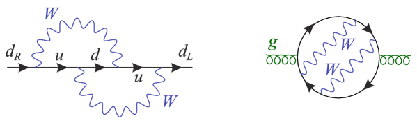
Figure 4: Leading electroweak contributions to $\theta_{eff}^{C}$, as arising either from complex quark mass renormalization or gluon propagation.

From Eq. (24), the $\mathcal{CP}$-violating $d$-quark mass correction must be tuned by

$$\Delta\theta_{eff}^{d\ quark}\sim\mathbf{[Y}_{u}^{\dagger}\mathbf{Y}_{u}\;,\;\mathbf{Y}_{u}^{\dagger}\mathbf{Y}_{u}\mathbf{Y}_{d}^{\dagger}\mathbf{Y}_{d}\mathbf{Y}_{u}^{\dagger}\mathbf{Y}_{u}]^{11}\;.$$ (47)

The total shift of the strong phase being the sum over the quark flavors, this contribution cancels exactly

$$\Delta\theta_{eff}^{d\ quark}+\Delta\theta_{eff}^{s\ quark}+\Delta\theta_{eff}^{b\ quark}=0\;,$$ (48)

and similarly for up-type quarks. This is nothing but the sum rule Eq. (32) originating from $\langle\mathbf{X}_{d}\rangle=0$. Actually, in the absence of strong interaction effects and at the mass insertion level, the leading contribution to $\Delta\theta_{eff}^{all\,quarks}$ must necessarily arise from

$$\Delta\theta_{eff}^{d\ quark}\sim((\mathbf{Y}_{d}^{\dagger}\mathbf{Y}_{d}\mathbf{)}^{2}\mathbf{Y}_{u}^{\dagger}\mathbf{Y}_{u}\mathbf{Y}_{d}^{\dagger}\mathbf{Y}_{d}(\mathbf{Y}_{u}^{\dagger}\mathbf{Y}_{u})^{2}-(\mathbf{Y}_{u}^{\dagger}\mathbf{Y}_{u})^{2}\mathbf{Y}_{d}^{\dagger}\mathbf{Y}_{d}\mathbf{Y}_{u}^{\dagger}\mathbf{Y}_{u}(\mathbf{Y}_{d}^{\dagger}\mathbf{Y}_{d}\mathbf{)}^{2})^{11}\;,$$ (49)

and thus the sum over the three flavors $d,s,b$ gives $\Delta\theta_{eff}^{quarks}\sim J_{\mathcal{CP}}\sim\Delta\theta_{eff}^{gluon}$. This observation was made in Ref. [32], in the context of the study of the leading divergent electroweak contribution to $\theta^{eff}$.

In the real world, the sum rule may be upset by strong corrections, as these soften the quadratic GIM breaking into logarithmic dependences on the quark masses. In Ref. [33], the leading contribution was found to arise at $\mathcal{O}(\alpha_{S}^{3})$, so we build the tentative estimate

$$\Delta\theta_{eff}^{quarks}\sim\left(\frac{g^{2}}{4\pi^{2}}\right)^{2}\left(\frac{\alpha_{S}}{\pi}\right)^{3}\max_{i}|\mathbf{X}_{d}^{ii}|\approx\left(\frac{g^{2}}{4\pi^{2}}\right)^{2}\left(\frac{\alpha_{S}}{\pi}\right)^{3}\frac{m_{b}^{2}m_{c}^{2}m_{t}^{4}}{M_{W}^{8}}\mathcal{J}_{\mathcal{CP}}\approx 10^{-16}\;.$$ (50)

An exact computation at that order has not yet been done though. At this stage, we should mention also the evaluation of Ref. [34], in which long-distance contributions are estimated by matching the $\eta^{(\prime)}\rightarrow\pi\pi$ rates induced by $\theta^{eff}$ to that obtained at the second order in the weak interaction, with the result $\Delta\theta_{eff}^{LD}\approx 10^{-17}$.

3.4 New Physics impact on quark and lepton EDM under MFV

In this section, we assume the existence of NP, but impose MFV, so the whole flavor sector remains tuned by the Yukawa couplings only. If we further assume that the rest of the NP dynamics respects $\mathcal{CP}$, the same combinations of spurions as in the SM are relevant to describe all flavor-diagonal $\mathcal{CP}$ violation.

Though analytically identical, three effects alter the numerical estimations. First, the NP dynamics can be far less restrictive than the SM, and these combinations of spurions can a priori arise from simpler diagrams. Second, the value of the Yukawa couplings can be different if more than one Higgs multiplet is present. For definiteness, we consider a THDM of Type II, in which Eq. (7) reads

$$v_{u}\mathbf{Y}_{u}\overset{frozen}{\rightarrow}\mathbf{m}_{u}V_{CKM},\;\;v_{d}\mathbf{Y}_{d}\overset{frozen}{\rightarrow}\mathbf{m}_{d},\;\;v_{d}\mathbf{Y}_{e}\overset{frozen}{\rightarrow}\mathbf{m}_{e}\;,$$ (51)

with $\tan\beta=v_{u}/v_{d}$ and $v_{u,d}=\langle H_{u,d}^{0}\rangle$ the vacuum expectation values of the two neutral scalars. When $\tan\beta$ is large, $\mathbf{Y}_{d}$ gets as large as $\mathbf{Y}_{u}$, and

$$J_{\mathcal{CP}}^{NP}\approx 10^{-12}\times\left(\frac{\tan\beta}{50}\right)^{6}\;\;,\;\;\;[\mathbf{X}_{d}^{NP}]^{11}\approx 10^{-9}\times\left(\frac{\tan\beta}{50}\right)^{2}\;\;,\;\;\;[\mathbf{X}_{u}^{NP}]^{11}\approx 10^{-7}\times\left(\frac{\tan\beta}{50}\right)^{6}\,\;.$$ (52)

Third, the scale appearing in Eq. (1) should be above the EW scale, and is tentatively set at $1$ TeV.

Combining these three numerical effects, and assuming the EDM are induced already at one loop, the predictions for the flavored contributions are

$$d_{e} \sim e\frac{m_{e}}{\Lambda^{2}}\left(\frac{g^{2}}{16\pi^{2}}\right)J_{\mathcal{CP}}^{NP}\approx 10^{-37}\times\left(\frac{1\,TeV}{\Lambda}\right)^{2}\times\left(\frac{\tan\beta}{50}\right)^{6}\;e\cdot cm\;,$$ (53a)

$$d_{d} \sim e\frac{m_{d}}{\Lambda^{2}}\left(\frac{g^{2}}{16\pi^{2}}\right)[\mathbf{X}_{d}^{NP}]^{11}\approx 10^{-33}\times\left(\frac{1\,TeV}{\Lambda}\right)^{2}\times\left(\frac{\tan\beta}{50}\right)^{2}\,\;e\cdot cm\;,$$ (53b)

$$d_{u} \sim e\frac{m_{u}}{\Lambda^{2}}\left(\frac{g^{2}}{16\pi^{2}}\right)[\mathbf{X}_{u}^{NP}]^{11}\approx 10^{-32}\times\left(\frac{1\,TeV}{\Lambda}\right)^{2}\times\left(\frac{\tan\beta}{50}\right)^{6}\,\;e\cdot cm\;.$$ (53c)

This corresponds to the situation for example in the MSSM for the contributions coming from the $$\mathcal{CP} \tan\beta$$-violating phases present in the squark flavor couplings (once MFV is imposed, see Ref. [15]). Note that as increases, these contributions scale as

$$\frac{|d_{d}|}{m_{d}}\approx 10^{3}\times\left(\frac{50}{\tan\beta}\right)^{4}\times\frac{|d_{e}|}{m_{e}}\;,\;\;\frac{|d_{u}|}{m_{u}}\sim 10^{5}\times\frac{|d_{e}|}{m_{e}}\;.$$ (54)

Given current bounds, $d_{e}$ and $d_{n}$ are then similarly sensitive to the $\mathcal{CP}$-violating phase at large $\tan\beta$, and clearly none of them is within range of the current and foreseeable experiments.

Besides these direct contributions to the EDM, similar loops shift $\theta_{eff}^{C}$. The main difference is the non-decoupling nature of these contributions, since they can come directly from the gluon or quark self-energies. Specifically,

$$\Delta\theta_{eff}^{gluon}\sim\left(\frac{g^{2}}{4\pi^{2}}\right)J_{\mathcal{CP}}^{NP}\approx 10^{-14}\times\left(\frac{\tan\beta}{50}\right)^{6}\;,$$ (55)

which is more constraining than the direct contributions Eq. (53), though still compatible with $\theta_{eff}^{C}\lesssim 10^{-10}$. Remember though that if a mechanism is introduced to solve the SM strong $\mathcal{CP}$ puzzle by forcing $\theta_{eff}^{C}=0$, for example by introducing the axion, then this same mechanism also kills $\Delta\theta_{eff}^{gluon}$, and Eqs. (53) come back as the leading contribution to the EDMs.

From the quark self-energies, the shift in $\theta_{eff}^{C}$ can be estimated as

$$\Delta\theta_{eff}^{d-quarks} \sim\left(\frac{g^{2}}{4\pi^{2}}\right)[\mathbf{X}_{d}^{NP}]^{11}\approx 10^{-11}\times\left(\frac{\tan\beta}{50}\right)^{2}\;,$$ (56)

$$\Delta\theta_{eff}^{u-quarks} \sim\left(\frac{g^{2}}{4\pi^{2}}\right)[\mathbf{X}_{u}^{NP}]^{11}\approx 10^{-10}\times\left(\frac{\tan\beta}{50}\right)^{6}\;.$$ (57)

These contributions would push $\theta_{eff}^{C}$ very close to its current bound from the neutron EDM. However, we still need to sum over the three flavors. At that stage, large cancellations can be expected. First, the spurion insertions do not necessarily come from quark mass insertions. For example, in a supersymmetric context, they could originate directly from the squark soft-breaking terms on which one imposes MFV. Alternatively, starting from universal boundary conditions, they would arise from the RG evolution down to the low scale. Second, the dynamical splitting of the contributions of each flavor would presumably not be as effective as in the SM. In the MSSM with MFV, squarks of a given type can be close to degenerate. For these reasons, one would actually expect the sum rule Eq. (48) to hold, at least to a good approximation, and thus that $\Delta\theta_{eff}^{quarks}\approx\Delta\theta_{eff}^{gluon}$ of Eq. (55), which is beyond our reach.

4 How to predict the EDM in the presence of neutrino masses?

In general, to account for neutrino masses, the SM dynamics must be supplemented with new flavored interactions. The minimal spurion content used up to now must thus be extended by some neutrino-related spurions. Further, this spurion content depends on the scenario adopted to generate the neutrino masses. So, starting again from the three magnetic operators Eq. (1), the goal of this section is to analyze the parametrization of $\mathbf{X}_{u,d,e}$ in the presence of the new spurions arising in the simplest neutrino mass generation scenarios.

A few general features can be immediately identified. First, the contributions to the up (down) quark EDM from the first (second) operators necessitate $\mathbf{X}_{u(d)}$ to be complex in the basis in which $\mathbf{Y}_{u(d)}$ is diagonal and real. As the quark and lepton flavor group remain factorized in all the scenarios considered here, $\mathbf{X}_{u,d}$ must be the identity times some flavor-invariant trace over the leptonic spurions. The quark EDM then arise only when these traces are complex, that is, when

$$\mathbf{X}_{u,d}=\mathbf{1}\times J_{\mathcal{CP}}\;\rightarrow d_{u,d}\sim e\frac{c_{u,d}}{\Lambda^{2}}m_{u,d}\times\operatorname{Im}J_{\mathcal{CP}}\;,$$ (58)

with $\operatorname{Im}J_{\mathcal{CP}}\neq 0$. Such $\mathcal{CP}$-violating flavor invariant traces have already been extensively studied in the literature for several neutrino mass scenarios (see in particular Ref. [6]), but will nevertheless be included in the following for completeness. Because the $\mathcal{CP}$-violating phase comes from a flavor invariant, and with $c_{u,d}$ some flavor blind combinations of gauge couplings and loop factors, we expect the relations

$$\frac{d_{u}}{m_{u}}=\frac{d_{c}}{m_{c}}=\frac{d_{t}}{m_{t}}=\frac{d_{d}}{m_{d}}=\frac{d_{s}}{m_{s}}=\frac{d_{b}}{m_{b}}\;,$$ (59)

to hold, up to subleading dependences on the loop particle masses.

For the lepton magnetic operator, on the other hand, $\mathbf{X}_{e}$ must be a chain of leptonic spurions transforming as an octet under $SU(3)_{L}$. In the basis in which $\mathbf{Y}_{e}$ is diagonal and real, it then induces the lepton flavor violating process $\ell^{I}\rightarrow\ell^{J}\gamma$ whenever it is non-diagonal, $\mathbf{X}_{e}^{IJ}\neq 0$, with rate

$$\Gamma\left(\ell^{I}\rightarrow\ell^{J}\gamma\right)=\frac{\alpha m_{\ell^{I}}^{5}c_{e}^{2}}{8\Lambda^{4}}\times|\mathbf{X}_{e}^{IJ}|^{2}\;,$$ (60)

and lepton EDM $d_{\ell^{I}}$ whenever its diagonal entries are complex, $\operatorname{Im}\mathbf{X}_{e}^{II}\neq 0$:

$$d_{e}\sim e\frac{c_{e}}{\Lambda^{2}}m_{e}\times\operatorname{Im}\mathbf{X}_{e}^{11}\;.$$ (61)

Typically, the dominant contribution to $d_{\ell}$ comes for a spurion chain such that $\langle\mathbf{X}_{e}\rangle=0$, hence the following sum rule holds:

$$\frac{d_{e}}{m_{e}}+\frac{d_{\mu}}{m_{\mu}}+\frac{d_{\tau}}{m_{\tau}}=0\;.$$ (62)

4.1 Dirac neutrino masses

Neutrino masses are trivial to introduce in the SM: it suffices to add three right handed neutrinos together with an additional Yukawa interaction:

$$\mathcal{L}_{\text{Yukawa}}=-\bar{U}\mathbf{Y}_{u}QH^{\dagger C}-\bar{D}\mathbf{Y}_{d}QH^{\dagger}-\bar{E}\mathbf{Y}_{e}LH^{\dagger}-\bar{N}\mathbf{Y}_{\nu}LH^{\dagger C}+h.c.\;.$$ (63)

These right-handed neutrinos have trivial gauge quantum numbers, $N\sim(\mathbf{1},\mathbf{1})_{0}$ under $SU(3)_{C}\otimes SU(2)_{L}\otimes U(1)_{Y}$. In the presence of $\mathbf{Y}_{\nu}$, it is no longer possible to get rid of all the flavor mixings in the lepton sector. The SVD of $\mathbf{Y}_{e}$ and $\mathbf{Y}_{\nu}$ are $vV_{R}^{e}\mathbf{Y}_{e}V_{L}^{e}=\mathbf{m}_{e}$ and $vV_{R}^{\nu}\mathbf{Y}_{\nu}V_{L}^{\nu}=\mathbf{m}_{\nu}$, and the mismatch between the left rotations defines the PMNS matrix [35]

$$U_{PMNS}^{\mathrm{Dirac}}\equiv V_{L}^{e\dagger}V_{L}^{\nu}\;.$$ (64)

With this, the background values of the spurions in the charged lepton mass eigenstate basis are

$$v\mathbf{Y}_{e}\overset{frozen}{\rightarrow}\mathbf{m}_{e}\;,\;v\mathbf{Y}_{\nu}\overset{frozen}{\rightarrow}\mathbf{m}_{\nu}U_{PMNS}^{\mathrm{Dirac}\dagger}\;.$$ (65)

The values of the various free parameters, as extracted from neutrino oscillation data, are taken from the best fit of Ref. [36]:

$$\Delta m_{21}^{2} =\Delta m_{\odot}^{2}=7.5_{-0.17}^{+0.19}\times 10^{-5}\,\text{eV}^{2},\;|\Delta m_{31}^{2}|=\Delta m_{atm}^{2}=2.524_{-0.040}^{+0.039}\times 10^{-3}\,\text{eV}^{2}\;,$$

$$\theta_{12} =\theta_{\odot}=(33.56_{-0.75}^{+0.77}){{}^{\circ}},\;\theta_{23}=\theta_{atm}=(41.6_{-1.2}^{+1.5}){{}^{\circ}},\;\theta_{13}=(8.46\pm 0.15){{}^{\circ}}\;,$$ (66)

for normal mass hierarchy which we shall assume in this paper. From here on, the predictions for the leptonic FCNC or the PMNS phase contributions to the EDMs is in strict parallel to that in Section 2. To set the stage for the following sections, let us nevertheless work them out explicitly.

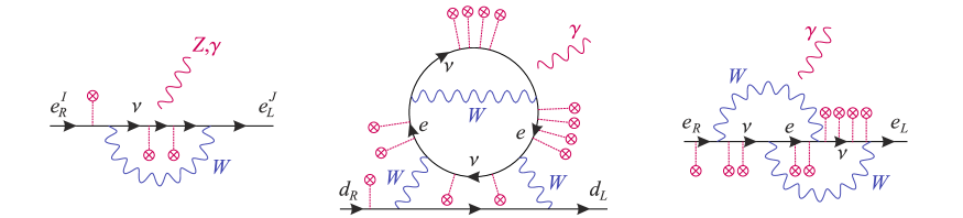
Figure 5: Examples of dominant spurion insertions for the LFV transitions $\ell^{I}\rightarrow\ell^{J}\gamma$, quark EDM, and lepton EDM, when the neutrino masses are purely of the Dirac type.

Lepton flavor violation:

In the SM supplemented by a Dirac neutrino mass term, $\mu\rightarrow e\gamma$ arise from virtual exchanges of the $W$ (see Fig. 5), and can be parametrized by the effective dimension-six magnetic operator Eq. (1) setting

$$\frac{c_{e}}{\Lambda^{2}}=\frac{G_{F}}{16\pi^{2}\sqrt{2}}\;\;,\;\;\mathbf{X}_{e}^{\mathrm{Dirac}}=\mathbf{1}\oplus\mathbf{Y}_{\nu}^{\dagger}\mathbf{Y}_{\nu}\oplus\mathbf{Y}_{e}^{\dagger}\mathbf{Y}_{e}+...\;,$$ (67)

where $\oplus$ serves as a reminder that in principle, $\mathcal{O}(1)$ coefficients appear in front of each term. In the charged lepton mass eigenstate basis, the dominant contribution comes from $\mathbf{Y}_{\nu}^{\dagger}\mathbf{Y}_{\nu}$. Freezing the spurions as in Eq. (65) and under the tribimaximal approximation, the decay rates are predicted as ($\lambda_{\ell}=\tau_{\ell}G_{F}^{2}\alpha m_{\ell}^{5}/2048\pi^{4}$)

$$\mathcal{B}\left(\mu\rightarrow e\gamma\right) \approx\lambda_{\mu}\left|\Delta m_{\odot}^{2}/3v^{2}\right|^{2}\approx 10^{-58}\;,\;\;\;[\mathcal{B}^{\exp}<5.7\times 10^{-13}\;\text{\cite[cite]{[\@@bibref{}{ExpMEG}{}{}]}}]\;,$$ (68a)

$$\mathcal{B}\left(\tau\rightarrow e\gamma\right) \approx\lambda_{\tau}\left|\Delta m_{\odot}^{2}/3v^{2}\right|^{2}\approx 10^{-59}\;,\;\;\;[\mathcal{B}^{\exp}<3.3\times 10^{-8}\;\text{\cite[cite]{[\@@bibref{}{ExpTLG}{}{}]}}]\;,$$ (68b)

$$\mathcal{B}\left(\tau\rightarrow\mu\gamma\right) \approx\lambda_{\tau}\left|\Delta m_{atm}^{2}/2v^{2}\right|^{2}\approx 10^{-49}\;,\;[\mathcal{B}^{\exp}<4.4\times 10^{-8}\;\text{\cite[cite]{[\@@bibref{}{ExpTLG}{}{}]}}]\;,$$ (68c)

which are prohibitively small, well beyond planned experimental sensitivities. Note that because of the GIM mechanism, what matter are the mass differences of the particles in the electroweak loop.

Quark EDMs:

They are induced by the flavor invariant traces over the leptonic spurions, see Fig. 5. In complete analogy to the CKM contribution to the lepton EDMs, we can immediately write

$$J_{\mathcal{CP}}^{\mathrm{Dirac}} \equiv\frac{1}{2i}\det[\mathbf{Y}_{e}^{\dagger}\mathbf{Y}_{e},\mathbf{Y}_{\nu}^{\dagger}\mathbf{Y}_{\nu}]=\frac{1}{2}\operatorname{Im}\langle(\mathbf{Y}_{\nu}^{\dagger}\mathbf{Y}_{\nu})^{2}\mathbf{Y}_{e}^{\dagger}\mathbf{Y}_{e}\mathbf{Y}_{\nu}^{\dagger}\mathbf{Y}_{\nu}(\mathbf{Y}_{e}^{\dagger}\mathbf{Y}_{e})^{2}\rangle$$

$$=\mathcal{J}_{\mathcal{CP}}^{\mathrm{Dirac}}\prod_{\begin{subarray}{c}i>j=e,\mu,\tau\\ i>j=\nu_{1},\nu_{2},\nu_{3}\end{subarray}}\frac{m_{i}^{2}-m_{j}^{2}}{v^{2}}\approx\mathcal{J}_{\mathcal{CP}}^{\mathrm{Dirac}}\frac{m_{\tau}^{4}m_{\mu}^{2}(\Delta m_{atm}^{2})^{2}\Delta m_{\odot}^{2}}{v^{12}}\approx 10^{-93}\sin(\delta_{13})\;,$$ (69)

with $\mathcal{J}_{\mathcal{CP}}^{\mathrm{Dirac}}$ given by the same expression as for the Jarlskog invariant of Eq. (19). Numerically, $\mathcal{J}_{\mathcal{CP}}^{\mathrm{Dirac}}\approx 0.033(2)\times\sin(\delta_{13})$ is not so far from its maximal value of $1/6\sqrt{3}\approx 0.096$ when $\delta_{13}$ is $\mathcal{O}(1)$, but $J_{\mathcal{CP}}^{\mathrm{Dirac}}$ is heavily suppressed by the $\mathcal{O}(m_{\nu}^{6})$ dependence and cannot compete with the CKM contributions to $d_{u,d}$.

Lepton EDMs:

The combination $\mathbf{X}_{e}$ in Eq. (1) should be a chain of spurions with complex diagonal entries. It is very similar to that for the quarks since the CH identity permit to construct the equivalent of the basis of Eq. (23), with $\mathbf{Y}_{\nu}^{\dagger}\mathbf{Y}_{\nu}$ and $\mathbf{Y}_{e}^{\dagger}\mathbf{Y}_{e}$ instead of $\mathbf{Y}_{u}^{\dagger}\mathbf{Y}_{u}$ and $\mathbf{Y}_{d}^{\dagger}\mathbf{Y}_{d}$. The simplest non-hermitian chain is thus

$$\mathbf{X}_{e}^{\mathrm{Dirac}}=[\mathbf{Y}_{\nu}^{\dagger}\mathbf{Y}_{\nu}\;,\;\mathbf{Y}_{\nu}^{\dagger}\mathbf{Y}_{\nu}\mathbf{Y}_{e}^{\dagger}\mathbf{Y}_{e}\mathbf{Y}_{\nu}^{\dagger}\mathbf{Y}_{\nu}]\;,$$ (70)

and corresponds to the second-order weak rainbow processes depicted in Fig. 5. For the electron EDM, it simplifies to

$$(\mathbf{X}_{e}^{\mathrm{Dirac}})^{11}=2i\mathcal{J}_{\mathcal{CP}}^{\mathrm{Dirac}}\;\frac{m_{\tau}^{2}-m_{\mu}^{2}}{v^{2}}\prod_{i>j=\nu_{1},\nu_{2},\nu_{3}}\frac{m_{i}^{2}-m_{j}^{2}}{v^{2}}\approx\mathcal{J}_{\mathcal{CP}}^{\mathrm{Dirac}}\;\frac{m_{\tau}^{2}(\Delta m_{atm}^{2})^{2}\Delta m_{\odot}^{2}}{v^{8}}\approx 10^{-82}\sin(\delta_{13})\;,$$ (71)

which translate into $d_{e}\lesssim 10^{-107}$ $e\cdot cm$. This is only marginally larger than the contribution proportional to $J_{\mathcal{CP}}^{\mathrm{Dirac}}$, Eq. (69), and much smaller than the CKM-induced contribution, Eq. (20). In addition, as for the quarks, this invariant cannot arise from two-loop diagrams, and the price to pay for an additional loop is an electromagnetic correction. Finally, the sum rule Eq. (62) holds since $\langle\mathbf{X}_{e}^{\mathrm{Dirac}}\rangle=0$. Actually, we even have $d_{e}/m_{e}\approx-d_{\mu}/m_{\mu}$ because $d_{\tau}/m_{\tau}$ is proportional to $m_{\mu}^{2}-m_{e}^{2}$ instead of $m_{\tau}^{2}-m_{\mu,e}^{2}\approx m_{\tau}^{2}$ for $d_{e,\mu}$.

For Dirac neutrinos, there is also the possibility to induce neutrino EDM from the operator $\bar{N}^{I}(\mathbf{Y}_{\nu}\mathbf{X}_{\nu})^{IJ}\sigma_{\mu\nu}L^{J}F^{\mu\nu}H$. The chain of spurions $\mathbf{X}_{\nu}^{\mathrm{Dirac}}$ is obtained from $\mathbf{X}_{e}^{\mathrm{Dirac}}$ in Eq. (70) by interchanging $\mathbf{Y}_{\nu}\leftrightarrow\mathbf{Y}_{e}$, and going to the gauge basis where neutrinos are mass eigenstates. It is strongly enhanced by the mass factors, with for example

$$\frac{d_{\nu_{1}}}{d_{e}}=-\frac{m_{\nu_{1}}(m_{\tau}^{2}-m_{e}^{2})(m_{\mu}^{2}-m_{e}^{2})}{m_{e}\Delta m_{atm}^{2}\Delta m_{\odot}^{2}}\approx 10^{36}\;,$$ (72)

for $m_{\nu_{1}}\approx 1$ eV, but is nevertheless totally out of reach experimentally [39].

4.2 Majorana neutrino masses

Instead of introducing right-handed neutrinos, the left-handed neutrinos can be directly given a gauge-invariant but lepton-number violating mass term as

$$\mathcal{L}_{\text{Yukawa}}=-\bar{U}\mathbf{Y}_{u}QH^{\dagger C}-\bar{D}\mathbf{Y}_{d}QH^{\dagger}-\bar{E}\mathbf{Y}_{e}LH^{\dagger}-\frac{1}{2v}(L^{I}H)\left(\mathbf{\Upsilon}_{\nu}\right)^{IJ}(L^{J}H)+h.c.\;.$$ (73)

The non-renormalizable dimension five coupling, called the Weinberg operator [40], collapses to a Majorana mass term $v\left(\mathbf{\Upsilon}_{\nu}\right)^{IJ}\nu_{L}^{I}\nu_{L}^{J}$ when the Higgs field acquire its vacuum expectation value. As in the Dirac case, there are thus only two elementary spurions at low energy. To fix their background values, first note that the unitary rotations needed to get from gauge to mass eigenstates are $vV_{R}^{e}\mathbf{Y}_{e}V_{L}^{e}=\mathbf{m}_{e}$ and $vV_{L}^{\nu T}\mathbf{\Upsilon}_{\nu}V_{L}^{\nu}=\mathbf{m}_{\nu}$ where $\mathbf{m}_{\nu}=\operatorname{diag}(m_{\nu 1},m_{\nu 2},m_{\nu 3})$ are the (real) neutrino masses. Only one matrix $V_{L}^{\nu}$ appears because $\mathbf{\Upsilon}_{\nu}$ is symmetric in flavor space. Choosing to rotate the lepton doublet by $V_{L}^{e}$, we can reach the gauge basis in which

$$v\mathbf{Y}_{e}\overset{frozen}{\rightarrow}\mathbf{m}_{e},\;\;\;v\mathbf{\Upsilon}_{\nu}\overset{frozen}{\rightarrow}V_{L}^{eT}V_{L}^{\nu\ast}\mathbf{m}_{\nu}V_{L}^{\nu\dagger}V_{L}^{e}\equiv U_{PMNS}^{\ast}\mathbf{m}_{\nu}U_{PMNS}^{\dagger}\;,$$ (74)

where $U_{PMNS}\equiv V_{L}^{e\dagger}V_{L}^{\nu}$ is related to the PMNS matrix as

$$U_{PMNS}=U_{PMNS}^{\mathrm{Dirac}}\cdot\operatorname{diag}(1,e^{i\alpha_{M}},e^{i\beta_{M}})\;.$$ (75)

Contrary to the Dirac case, these phases cannot be rotated away, essentially because lepton number is no longer conserved. One of the extra phases is conventionally eliminated as an irrelevant global phase, while the two others are called Majorana phases.

Lepton flavor violation:

If neutrinos are purely Majorana particles, LFV processes are encoded in the operator Eq. (1) with $\mathbf{X}_{e}$ given by

$$\mathbf{X}_{e}^{\mathrm{Majo}}=\mathbf{\Upsilon}_{\nu}^{\dagger}\mathbf{\Upsilon}_{\nu}\;.$$ (76)

This is depicted in Fig. 6. This mechanism produces the same amplitudes as in the Dirac neutrino case since

$$\mathbf{\Upsilon}_{\nu}^{\dagger}\mathbf{\Upsilon}_{\nu}=\frac{1}{v^{2}}U_{PMNS}\mathbf{m}_{\nu}^{2}U_{PMNS}^{\dagger}=(\mathbf{Y}_{\nu}^{\dagger}\mathbf{Y}_{\nu})^{\mathrm{Dirac}}\;,$$ (77)

and the rates in $\Delta m_{\nu}^{4}$ are the same as in Eq. (68).

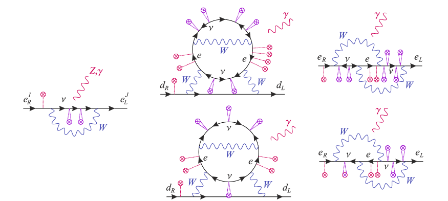
Figure 6: Examples of spurion insertions for the LFV transitions, quark and lepton EDMs for purely Majorana neutrinos. The double tadpoles denote Majorana mass insertions, while the single ones denote charged lepton Yukawa couplings. Diagrams on top depict the Jarlskog-like combinations Eq. (79) and (83), while that on the bottom show those specific to the Majorana case, Eq. (80) and (84).

Quark EDMs:

The spurion $\mathbf{\Upsilon}_{\nu}$ is not transforming in the same way as the other Yukawa couplings and this opens many new ways of contracting the spurions to form $G_{F}$ invariants. To organize the expansion, first note that thanks to CH identities, any chain of spurions transforming as an octet under $SU(3)_{L}$ is necessarily a combination of only four elementary hermitian monomials, also transforming as octets under $SU(3)_{L}$:

$$\mathbf{Y}_{e}^{\dagger}\mathbf{Y}_{e}\;,\;\;\mathbf{\Upsilon}_{\nu}^{\dagger}\mathbf{\Upsilon}_{\nu}\;,\;\;\mathbf{\Upsilon}_{\nu}^{\dagger}(\mathbf{Y}_{e}^{\dagger}\mathbf{Y}_{e})^{T}\mathbf{\Upsilon}_{\nu}\;,\;\;\mathbf{\Upsilon}_{\nu}^{\dagger}((\mathbf{Y}_{e}^{\dagger}\mathbf{Y}_{e})^{T})^{2}\mathbf{\Upsilon}_{\nu}\;.$$ (78)

The CH identities also imply that the simplest purely imaginary invariant built out of only two hermitian spurion combinations $\mathbf{A}$ and $\mathbf{B}$ is necessarily $\det[\mathbf{A},\mathbf{B}]$. With three different spurion combinations, the simplest complex invariant is $\langle\mathbf{ABC}-\mathbf{CBA}\rangle$, while with four, there are a priori many new invariants.

Specifically, given the set of octet spurion combinations, the analogue of the Dirac invariant does not bring anything new since Eq. (77) holds:

$$J_{\mathcal{CP}}^{\mathrm{Majo,1}}=\frac{1}{2i}\det[\mathbf{Y}_{e}^{\dagger}\mathbf{Y}_{e},\mathbf{\Upsilon}_{\nu}^{\dagger}\mathbf{\Upsilon}_{\nu}]=J_{\mathcal{CP}}^{\mathrm{Dirac}}\;.$$ (79)

Sensitivity to the Majorana phases is lost in $\mathbf{\Upsilon}_{\nu}^{\dagger}\mathbf{\Upsilon}_{\nu}$. By trial and error, the simplest invariant sensitive to these phases is found to be [6, 41]

$$J_{\mathcal{CP}}^{\mathrm{Majo,2}}=\frac{1}{2i}\langle\mathbf{\Upsilon}_{\nu}^{\dagger}\mathbf{\Upsilon}_{\nu}\cdot\mathbf{Y}_{e}^{\dagger}\mathbf{Y}_{e}\cdot\mathbf{\Upsilon}_{\nu}^{\dagger}(\mathbf{Y}_{e}^{\dagger}\mathbf{Y}_{e})^{T}\mathbf{\Upsilon}_{\nu}-\mathbf{\Upsilon}_{\nu}^{\dagger}(\mathbf{Y}_{e}^{\dagger}\mathbf{Y}_{e})^{T}\mathbf{\Upsilon}_{\nu}\cdot\mathbf{Y}_{e}^{\dagger}\mathbf{Y}_{e}\cdot\mathbf{\Upsilon}_{\nu}^{\dagger}\mathbf{\Upsilon}_{\nu}\rangle\;.$$ (80)

Though this purely imaginary quantity vanishes when all charged lepton or neutrinos have equal masses, it does not if only two leptons or neutrinos are degenerate. As a result, a simple product of mass differences cannot be factored out and this invariant does not have a simple analytical expression.

If we are after an invariant which does not vanish for degenerate neutrinos, we must avoid any chain in which $\mathbf{\Upsilon}_{\nu}^{\dagger}\mathbf{\Upsilon}_{\nu}$ or $\mathbf{\Upsilon}_{\nu}\mathbf{\Upsilon}_{\nu}^{\dagger}=(\mathbf{\Upsilon}_{\nu}^{\dagger}\mathbf{\Upsilon}_{\nu})^{T}$ factors appears, since $\mathbf{\Upsilon}_{\nu}^{\dagger}\mathbf{\Upsilon}_{\nu}=\mathbf{\Upsilon}_{\nu}\mathbf{\Upsilon}_{\nu}^{\dagger}=(m_{\nu}^{2}/v^{2})\mathbf{1}$ in the degenerate limit. This means that all occurrences of $\mathbf{\Upsilon}_{\nu}$ or $\mathbf{\Upsilon}_{\nu}^{\dagger}$ must be between powers of $\mathbf{Y}_{e}^{\dagger}\mathbf{Y}_{e}$ or $(\mathbf{Y}_{e}^{\dagger}\mathbf{Y}_{e})^{T}$. The simplest such invariants are

$$J_{\mathcal{CP}}^{\mathrm{Majo,3}} =\operatorname{Im}\langle(\mathbf{Y}_{e}^{\dagger}\mathbf{Y}_{e}\mathbf{)}^{2}\cdot\mathbf{\Upsilon}_{\nu}^{\dagger}(\mathbf{Y}_{e}^{\dagger}\mathbf{Y}_{e})^{T}\mathbf{\Upsilon}_{\nu}\cdot\mathbf{Y}_{e}^{\dagger}\mathbf{Y}_{e}\cdot(\mathbf{\Upsilon}_{\nu}^{\dagger}(\mathbf{Y}_{e}^{\dagger}\mathbf{Y}_{e})^{T}\mathbf{\Upsilon}_{\nu})^{2}\rangle\;,$$ (81)

$$J_{\mathcal{CP}}^{\mathrm{Majo,4}} =\operatorname{Im}\langle(\mathbf{Y}_{e}^{\dagger}\mathbf{Y}_{e})^{2}\cdot\mathbf{\Upsilon}_{\nu}^{\dagger}(\mathbf{Y}_{e}^{\dagger}\mathbf{Y}_{e})^{T}\mathbf{\Upsilon}_{\nu}\cdot\mathbf{Y}_{e}^{\dagger}\mathbf{Y}_{e}\cdot\mathbf{\Upsilon}_{\nu}^{\dagger}((\mathbf{Y}_{e}^{\dagger}\mathbf{Y}_{e})^{2})^{T}\mathbf{\Upsilon}_{\nu}\rangle\;.$$ (82)

The invariant $2iJ_{\mathcal{CP}}^{\mathrm{Majo,3}}=\det[\mathbf{\Upsilon}_{\nu}^{\dagger}(\mathbf{Y}_{e}^{\dagger}\mathbf{Y}_{e})^{T}\mathbf{\Upsilon}_{\nu},\mathbf{Y}_{e}^{\dagger}\mathbf{Y}_{e}]$ was already found in Ref. [42], but it is not the largest one since $J_{\mathcal{CP}}^{\mathrm{Majo,3}}=(m_{\nu}^{2}/v^{2})\times J_{\mathcal{CP}}^{\mathrm{Majo,4}}$ in the degenerate limit. Note also that for both these invariants, the $(\mathbf{Y}_{e}^{\dagger}\mathbf{Y}_{e})^{2}$ factor has to appear instead of simply $(\mathbf{Y}_{e}^{\dagger}\mathbf{Y}_{e})$ because otherwise, the CH identities would allow to reorder terms as $\mathbf{A}\cdot\mathbf{B}\cdot\mathbf{A}\rightarrow-\mathbf{A}^{2}\cdot\mathbf{B}-\mathbf{B}\cdot\mathbf{A}^{2}+($less factors$)$, at which point $\mathbf{\Upsilon}_{\nu}^{\dagger}\mathbf{\Upsilon}_{\nu}$ or $\mathbf{\Upsilon}_{\nu}\mathbf{\Upsilon}_{\nu}^{\dagger}$ contractions would appear and the invariants would again vanish in the degenerate limit.

Lepton EDMs:

For each of the previous trace invariant, we can construct a corresponding non-hermitian chain of spurions. The reasoning is very similar to that in the Dirac case, and here also, at least four neutrino mass insertions are needed:

$$\mathbf{X}_{e}^{\mathrm{Majo,1}} =[\mathbf{\Upsilon}_{\nu}^{\dagger}\mathbf{\Upsilon}_{\nu}\;,\;\mathbf{\Upsilon}_{\nu}^{\dagger}\mathbf{\Upsilon}_{\nu}\mathbf{Y}_{e}^{\dagger}\mathbf{Y}_{e}\mathbf{\Upsilon}_{\nu}^{\dagger}\mathbf{\Upsilon}_{\nu}]\;,$$ (83)

$$\mathbf{X}_{e}^{\mathrm{Majo,2}} =[\mathbf{\Upsilon}_{\nu}^{\dagger}\mathbf{\Upsilon}_{\nu}\;,\;\mathbf{\Upsilon}_{\nu}^{\dagger}(\mathbf{Y}_{e}^{\dagger}\mathbf{Y}_{e})^{T}\mathbf{\Upsilon}_{\nu}]\;,$$ (84)

$$\mathbf{X}_{e}^{\mathrm{Majo,3}} =[\mathbf{\Upsilon}_{\nu}^{\dagger}((\mathbf{Y}_{e}^{\dagger}\mathbf{Y}_{e})^{2})^{T}\mathbf{\Upsilon}_{\nu}\;,\;\mathbf{Y}_{e}^{\dagger}\mathbf{Y}_{e}\cdot\mathbf{\Upsilon}_{\nu}^{\dagger}(\mathbf{Y}_{e}^{\dagger}\mathbf{Y}_{e})^{T}\mathbf{\Upsilon}_{\nu}\cdot\mathbf{Y}_{e}^{\dagger}\mathbf{Y}_{e}]\;,$$ (85)

$$\mathbf{X}_{e}^{\mathrm{Majo,4}} =\mathbf{\Upsilon}_{\nu}^{\dagger}((\mathbf{Y}_{e}^{\dagger}\mathbf{Y}_{e})^{2})^{T}\mathbf{\Upsilon}_{\nu}\cdot\mathbf{Y}_{e}^{\dagger}\mathbf{Y}_{e}\cdot\mathbf{\Upsilon}_{\nu}^{\dagger}(\mathbf{Y}_{e}^{\dagger}\mathbf{Y}_{e})^{T}\mathbf{\Upsilon}_{\nu}$$

$$\;\;\;\;\;\;\;\;\;-\mathbf{\Upsilon}_{\nu}^{\dagger}(\mathbf{Y}_{e}^{\dagger}\mathbf{Y}_{e})^{T}\mathbf{\Upsilon}_{\nu}\cdot\mathbf{Y}_{e}^{\dagger}\mathbf{Y}_{e}\cdot\mathbf{\Upsilon}_{\nu}^{\dagger}((\mathbf{Y}_{e}^{\dagger}\mathbf{Y}_{e})^{2})^{T}\mathbf{\Upsilon}_{\nu}\;.$$ (86)

These structures share many of the properties of $J_{\mathcal{CP}}^{\mathrm{Majo,1}}$ to $J_{\mathcal{CP}}^{\mathrm{Majo,4}}$. Due to Eq. (77), the combination $\mathbf{X}_{e}^{\mathrm{Majo,1}}$ reproduces the Dirac invariant of Eq. (70). The $\mathbf{X}_{e}^{\mathrm{Majo,2}}$ is specific to the Majorana case: it arises because there are more than two octet spurion combinations, and both $\mathbf{\Upsilon}_{\nu}^{\dagger}\mathbf{\Upsilon}_{\nu}$ and $\mathbf{\Upsilon}_{\nu}^{\dagger}(\mathbf{Y}_{e}^{\dagger}\mathbf{Y}_{e})^{T}\mathbf{\Upsilon}_{\nu}$ are non-diagonal in the gauge basis in which $\mathbf{Y}_{e}^{\dagger}\mathbf{Y}_{e}$ is diagonal. Further, as $J_{\mathcal{CP}}^{\mathrm{Majo,2}}$, it depends only quartically on the neutrino masses, is sensitive to the PMNS phase as well as to the two Majorana phases, has a very complicated analytical expression, but vanishes if either the three charged leptons or the three neutrinos are degenerate in mass. Other structures of this type can be constructed but they all involve more $\mathbf{Y}_{e}^{\dagger}\mathbf{Y}_{e}$ or $\mathbf{\Upsilon}_{\nu}^{\dagger}\mathbf{\Upsilon}_{\nu}$ insertions, and are thus more suppressed.

Finally, the last two $\mathbf{X}_{e}^{\mathrm{Majo,3}}$ and $\mathbf{X}_{e}^{\mathrm{Majo,4}}$ are the simplest combinations surviving in the strict degenerate neutrino mass limit, when $\mathbf{\Upsilon}_{\nu}^{\dagger}\mathbf{\Upsilon}_{\nu}\rightarrow(m_{\nu}^{2}/v^{2})\mathbf{1}$. In that case, note that $(\mathbf{X}_{e}^{\mathrm{Majo,3}})^{ii}=(m_{\ell^{i}}/v)^{2}\times(\mathbf{X}_{e}^{\mathrm{Majo,4}})^{ii}$ since the $\mathbf{X}_{e}^{\mathrm{Majo,3}}$ spurion chain ends or starts by the diagonal $\mathbf{Y}_{e}^{\dagger}\mathbf{Y}_{e}$ factor. Still, the sum rule Eq. (62) holds in both cases, since $\langle\mathbf{X}_{e}^{\mathrm{Majo,3}}\rangle=\langle\mathbf{X}_{e}^{\mathrm{Majo,4}}\rangle=0$.

Numerical estimates for the EDMs:

To estimate the size of the quark and lepton EDMs, several pieces must be combined. First, the spurion combinations are evaluated by plugging in the background values in Eq. (74). At this stage, the analytical expressions for most cases are far too complicated to be written down explicitly. Nevertheless, to illustrate the dependences on the various parameters, let us give an example. Consider $J_{\mathcal{CP}}^{\mathrm{Majo,2}}$ and keep only the leading terms in $\mathcal{O}(m_{\tau}^{4})$ and up to $\mathcal{O}(\sin\theta_{13})$:

$$\frac{1}{2i}J_{\mathcal{CP}}^{\mathrm{Majo,2}} =\frac{m_{\tau}^{4}}{v^{8}}s_{23}^{2}\left(s_{12}^{2}c_{12}^{2}s_{23}^{2}\mu_{12}^{4}\sin(2\alpha_{M})+s_{12}^{2}c_{23}^{2}\mu_{13}^{4}\sin(2\beta_{M})+c_{12}^{2}c_{23}^{2}\mu_{32}^{4}\sin(2(\alpha_{M}-\beta_{M}))\right)$$

$$\;\;\;\;+s_{13}\frac{2m_{\tau}^{4}}{v^{8}}c_{12}c_{23}s_{12}s_{23}^{3}\mu_{12}^{4}\left(s_{12}^{2}\sin(2\alpha_{M}+\delta_{13})-c_{12}^{2}\sin(2\alpha_{M}-\delta_{13})\right)$$

$$\;\;\;\;+s_{13}\frac{2m_{\tau}^{4}}{v^{8}}c_{12}c_{23}^{3}s_{23}s_{12}\left(\mu_{32}^{4}\sin(2\alpha_{M}-2\beta_{M}+\delta_{13})-\mu_{13}^{4}\sin(2\beta_{M}-\delta_{13})\right)\;,$$ (87)

where $\mu_{ab}^{4}=m_{\nu^{a}}m_{\nu^{b}}(m_{\nu^{a}}^{2}-m_{\nu^{b}}^{2})$ and $s_{ij}=\sin\theta_{ij}$, $c_{ij}=\cos\theta_{ij}$. This expression reproduces within 5% the exact expansion over the allowed range for the neutrino mass scale. Numerically, the $\mathcal{O}(\sin\theta_{13})$ term is subleading, but nevertheless relevant when the Majorana phases are sufficiently small (or close to exact angles) to allow the Dirac phase to contribute significantly. Except when $\alpha_{M}-\beta_{M}$ is close to $\pi/2$, the third term dominates, while the $\delta_{13}$ dependence comes essentially from the $\sin(2\beta_{M}-\delta_{13})$ and $\sin(2\alpha_{M}-2\beta_{M}+\delta_{13})$ terms. Note, finally, that the analytical expression of $(\mathbf{X}_{e}^{\mathrm{Majo,2}})^{11}$ is similar, and shares in particular the $\mu_{ab}^{4}$ dependences on neutrino masses (in agreement with the exact two-loop computations [43]), but depends differently on the $\mathcal{CP}$-violating phases. Explicitly, its leading terms in $\mathcal{O}(m_{\tau}^{2})$ and up to $\mathcal{O}(\sin\theta_{13})$,

$$\frac{1}{2i}(\mathbf{X}_{e}^{\mathrm{Majo,2}})^{11} =\frac{m_{\tau}^{2}}{v^{6}}s_{23}^{2}s_{12}^{2}c_{12}^{2}\mu_{12}^{4}\sin(2\alpha_{M})$$

$$+s_{13}\frac{m_{\tau}^{2}}{v^{6}}c_{12}c_{23}s_{12}s_{23}\mu_{12}^{4}\left(s_{12}^{2}\sin(2\alpha_{M}+\delta_{13})-c_{12}^{2}\sin(2\alpha_{M}-\delta_{13})\right)$$

$$+s_{13}\frac{m_{\tau}^{2}}{v^{6}}c_{12}c_{23}s_{23}s_{12}\left(\mu_{32}^{4}\sin(2\alpha_{M}-2\beta_{M}+\delta_{13})-\mu_{13}^{4}\sin(2\beta_{M}-\delta_{13})\right)\;.$$ (88)

In practice, as none of the leptonic $\mathcal{CP}$-violating phases are known, we quote in Table 1 the maximum absolute values attainable as $\delta_{13}$, $\alpha_{M}$, and $\beta_{M}$ are allowed to take any value. The large range of orders of magnitude spanned by the various combinations can be understood from their scalings in lepton and neutrino masses. Specifically, the lepton GIM mechanism is always effective and all spurion combinations vanish in the $m_{e}=m_{\mu}=m_{\tau}$ limit. In the more restricted case of two degenerate charged leptons, only $J_{\mathcal{CP}}^{\mathrm{Majo,1}}$ and $\mathbf{X}_{e}^{\mathrm{Majo,1}}$ vanish. On the other hand, the neutrino GIM mechanism is only effective for $\mathbf{\Upsilon}_{\nu}^{\dagger}\mathbf{\Upsilon}_{\nu}\rightarrow\mathcal{O}(\Delta m_{\nu}^{2}/v^{2})$, and absolute neutrino masses occur for $\mathbf{\Upsilon}_{\nu}^{\dagger}(\mathbf{Y}_{e}^{\dagger}\mathbf{Y}_{e})^{T}\mathbf{\Upsilon}_{\nu}\rightarrow\mathcal{O}(m_{\nu}^{2}m_{\ell}^{2}/v^{4})$ and $\mathbf{\Upsilon}_{\nu}^{\dagger}((\mathbf{Y}_{e}^{\dagger}\mathbf{Y}_{e})^{T})^{2}\mathbf{\Upsilon}_{\nu}\rightarrow\mathcal{O}(m_{\nu}^{2}m_{\ell}^{4}/v^{6})$. These behaviors are illustrated in Fig. 7.

Figure 7: Left: Evolutions of $J_{CP}^{\mathrm{Majo,}i}$ and $(\mathbf{X}_{e}^{\mathrm{Majo,}i})^{11}$, $i=1,2,4$, as functions of the lightest neutrino mass $m_{\nu 1}$, normalized to their respective values for $m_{\nu 1}=1\,$eV. The case $i=1$ corresponds to the Jarlskog-like combinations Eqs. (79) and (83), and depends only on neutrino mass differences. The case $i=2$ depicts the simpler combinations Eqs. (80) and (84), and $i=4$ the dominant combinations surviving in the degenerate neutrino case, Eqs. (82) and (86). Right: Area spanned by $J_{CP}^{\mathrm{Majo,2}}$ and $(\mathbf{X}_{e}^{\mathrm{Majo,2}})^{11}$ for $m_{\nu 1}=1$ eV as the PMNS phase $\delta_{13}$ and the Majorana phases $\alpha_{M},\beta_{M}$ are allowed to take on any values. The lines show the strict correlation occurring when only one phase is non-zero. The misalignment of these three lines explains the decorrelation exhibited by the grey area.

If there is no new physics beyond a Majorana neutrino mass term, these flavor structures have to arise from electroweak interactions, see Fig. 6. The EW order at which this happens can be figured out by counting the number of charged current transitions, i.e., the contractions between $\mathbf{\Upsilon}_{\nu}$ and $\mathbf{Y}_{e}$ or their (hermitian) transpose, in the spurion chain. This also corresponds to the number of surviving PMNS matrices. To this, one weak order must be added for the quark EDM, since the closed lepton loop has to be connected to the hadronic current. Diagrams with three photons also contribute, but are of similar sizes as

$$\frac{g^{2}}{4\pi}\frac{1}{M_{W}^{2}}\approx\left(\frac{e^{2}}{4\pi}\right)^{3}\frac{1}{\Lambda_{had}^{2}}\approx 10^{-6}\;,$$ (89)

with $\Lambda_{had}$ the typical hadronic scale. Finally, for the first invariant $J_{\mathcal{CP}}^{\mathrm{Majo,1}}=J_{\mathcal{CP}}^{\mathrm{Dirac}}$ and its associated rainbow structure $\mathbf{X}_{e}^{\mathrm{Majo,1}}=\mathbf{X}_{e}^{\mathrm{Dirac}}$, at least an additional electroweak loop is required to get a non-vanishing results, in analogy to the CKM contributions in Eq. (20) and (28). By contrast, the electroweak loops for the Majorana case $J_{\mathcal{CP}}^{\mathrm{Majo,2}}$ and $\mathbf{X}_{e}^{\mathrm{Majo,2}}$ have different symmetry properties, and no extra loop is needed [43, 44]. A priori, the same is true for the degenerate cases, though this has not been checked explicitly. In any case, this is not relevant numerically since neutrinos being lighter than about $1$ eV, they are never degenerate enough to invert the strong hierarchy $J_{\mathcal{CP}}^{\mathrm{Majo,3}}\ll J_{\mathcal{CP}}^{\mathrm{Majo,4}}\ll J_{\mathcal{CP}}^{\mathrm{Majo,2}}$. The total EW orders at which we expect each spurion combination to arise are listed in Table 1.

	$m_{\nu 1}\lesssim 0.01$ eV		$m_{\nu 1}=1\,$eV		EDM scaling
	Only $\delta_{13}$	All	Only $\delta_{13}$	All	Flavor	Gauge	Prefactor [$e\cdot cm$]
$J_{\mathcal{CP}}^{\mathrm{Majo,1}}$	$10^{-93}$	$10^{-93}$	$10^{-93}$	$10^{-93}$	$\frac{(\Delta m_{\nu}^{2})^{3}(\Delta m_{\ell}^{2})^{3}}{v^{12}}$	$\alpha_{W}^{2+1+1}$	10-14
$J_{\mathcal{CP}}^{\mathrm{Majo,2}}$	$10^{-60}$	$10^{-59}$	$10^{-58}$	$10^{-56}$	$\frac{m_{\nu}^{2}\Delta m_{\nu}^{2}m_{\ell}^{4}}{v^{8}}$	$\alpha_{W}^{2+1}$	10-15
$J_{\mathcal{CP}}^{\mathrm{Majo,3}}$	$10^{-107}$	$10^{-107}$	$10^{-100}$	$10^{-97}$	$\frac{m_{\nu}^{6}m_{\ell}^{12}}{v^{18}}$	$\alpha_{W}^{5+1}$	10-12
$J_{\mathcal{CP}}^{\mathrm{Majo,4}}$	$10^{-83}$	$10^{-80}$	$10^{-77}$	$10^{-75}$	$\frac{m_{\nu}^{4}m_{\ell}^{12}}{v^{16}}$	$\alpha_{W}^{4+1}$	10-12
$(\mathbf{X}_{e}^{\mathrm{Majo,1}})^{11}$	$10^{-82}$	$10^{-82}$	$10^{-82}$	$10^{-82}$	$\frac{(\Delta m_{\nu}^{2})^{3}\Delta m_{\ell}^{2}}{v^{8}}$	$\alpha_{W}^{2+1}$	10-16
$(\mathbf{X}_{e}^{\mathrm{Majo,2}})^{11}$	$10^{-56}$	$10^{-56}$	$10^{-53}$	$10^{-53}$	$\frac{m_{\nu}^{2}\Delta m_{\nu}^{2}m_{\ell}^{2}}{v^{6}}$	$\alpha_{W}^{2}$	10-17
$(\mathbf{X}_{e}^{\mathrm{Majo,3}})^{11}$	$10^{-82}$	$10^{-82}$	$10^{-78}$	$10^{-75}$	$\frac{m_{\nu}^{4}m_{e}^{10}}{v^{14}}$	$\alpha_{W}^{4}$	10-14
$(\mathbf{X}_{e}^{\mathrm{Majo,4}})^{11}$	$10^{-71}$	$10^{-71}$	$10^{-67}$	$10^{-64}$	$\frac{m_{\nu}^{4}m_{\ell}^{8}}{v^{12}}$	$\alpha_{W}^{4}$	10-15

Table 1: Numerical estimates for the spurion combinations constructed in the previous sections. The values obtained do not change significantly when the lightest neutrino mass is below about 0.01 eV, see Fig. 7. In each case, the scaling in neutrino and lepton masses is indicated. The corresponding estimates for the quark and lepton EDM is obtained by multiplying the gauge factor, prefactor, and spurion combination.

As a final piece to estimate the EDMs, the chirality flips and the overall operator scale $\Lambda\approx M_{W}$ appearing in Eqs. (58) and (61) are combined into the prefactors quoted in Table 1. In addition, we also include in these prefactors the adequate power of $v/M_{W}$ to compensate for the normalization of the spurions, since in practice ratios of fermion masses over $M_{W}$ should arise from the electroweak loops. Of course, these order of magnitude estimates are to be understood as very approximate, since dynamical effects are neglected.

Having the flavor structures of both the lepton and quark EDMs, we can study their correlations. This is important since it tells us of the relative sensitivity of these EDMs to the underlying $\mathcal{CP}$-violating phases. For the Jarlskog-like structures $J_{\mathcal{CP}}^{\mathrm{Majo,1}}$ and $(\mathbf{X}_{e}^{\mathrm{Majo,1}})^{11}$, which does not depend on the overall neutrino mass scale or the Majorana phases, the ratio of the two expressions (see Eqs. (69) and (71)) is entirely fixed in terms of lepton masses

$$\frac{\operatorname{Im}(\mathbf{X}_{e}^{\mathrm{Dirac}})^{11}}{2J_{\mathcal{CP}}^{\mathrm{Dirac}}}=\frac{v^{4}}{(m_{\tau}^{2}-m_{e}^{2})(m_{\mu}^{2}-m_{e}^{2})}\approx 10^{11}\;.$$ (90)

On the contrary, for the Majorana cases, the presence of three separate sources of $\mathcal{CP}$-violation completely decorrelates the lepton and quark EDMs. In Fig. 7 is shown the result of a scan allowing $\delta_{13}$, $\alpha$, and $\beta$ to vary over their whole range and $m_{\nu 1}\in[0,1]$ eV. From this plot, it is apparent that even though the analytical expressions of $J_{\mathcal{CP}}^{\mathrm{Majo,2}}$ and $(\mathbf{X}_{e}^{\mathrm{Majo,2}})^{11}$ are similar, see Eqs. (87) and (88), their different dependences on the trigonometric functions has important consequences. Though it certainly requires some level of fine tuning, it is even possible to invert the hierarchy and get $J_{\mathcal{CP}}^{\mathrm{Majo,2}}>(\mathbf{X}_{e}^{\mathrm{Majo,2}})^{11}$. Enhancing the $d_{u,d}/d_{e}$ ratio in this way is bounded though. When $(\mathbf{X}_{e}^{\mathrm{Majo,2}})^{11}\lesssim J_{\mathcal{CP}}^{\mathrm{Majo,2}}$, the dominant contribution to the lepton EDM comes from $\mathbf{X}_{e}=\mathbf{1}\times J_{\mathcal{CP}}^{\mathrm{Majo,2}}$, see Eq. (58). It corresponds to the situation in which both the quark and lepton EDM are induced by the same closed lepton loop, see Fig. 6. Being tuned by the same invariant, and barring a fine-tuned cancellation between the rainbow and bubble contributions to $d_{e}$, the EDMs should obey

$$\frac{d_{d}}{m_{d}}\lesssim\frac{d_{e}}{m_{e}}\;.$$ (91)

Of course, all these values are well beyond the planned sensitivities, but we will discuss in the next section how to enhance these values and bring them within range of experiments.

4.3 Seesaw mechanisms

The background values for the neutrino spurions in both the Dirac and Majorana case are extremely suppressed, simply because neutrinos are very light. In turn, the spurion combinations tuning the LFV transitions or EDMs end up far too suppressed to make them accessible experimentally. From a theory perspective, these background values are too tiny to appear natural, and it is generally accepted that this suppression has a dynamical origin. After all, the Weinberg operator from which the small Majorana mass term originates is not renormalizable. If it arises at a very high scale, left-handed neutrinos would automatically be light. There are three ways to achieve this dynamically at tree level [45], depending on how to minimally extend the particle content of the SM. Type I seesaw introduces heavy weak singlet right-handed neutrinos [46], Type III seesaw is very similar to Type I but adds weak triplet right-handed neutrinos instead (Type III), while the Type II extends the scalar sector of the SM with a weak triplet of scalar fields [47].

Once the suppression of the neutrino masses is taken care of dynamically, what remain are far less suppressed flavor structures. Of course, in the absence of any NP, the only access at low-energy to these flavor structures is through the neutrino mass term, making them unobservable again. However, if we assume some NP exists not too far above the EW scale, then the unsuppressed neutrino flavor structures could directly impact LFV transitions and EDMs. It is the purpose of the present section to treat these scenarios using the tools designed in the previous sections.

4.3.1 Type II Seesaw mechanism

Introducing a scalar weak triplet $\Delta_{i}$, $i=1,2,3$ with hypercharge 2, the allowed renormalizable couplings are (see e.g. Ref. [48] for a detailed description)

$$\mathcal{L} =\mathcal{L}_{SM}+D_{\mu}\vec{\Delta}^{\dagger}\cdot D^{\mu}\vec{\Delta}-\vec{\Delta}^{\dagger}\vec{\Delta}M_{\Delta}^{2}-\delta V(H,\vec{\Delta})$$ (92)

$$\;\;\;\;\;\;\;+\frac{1}{2}(\bar{L}^{\mathrm{C}}\mathbf{\Upsilon}_{\Delta}\vec{\sigma}L+\lambda_{\Delta}M_{\Delta}H^{\dagger}\vec{\sigma}H^{\dagger})\cdot\vec{\Delta}+h.c.\;\;,$$ (93)

where $\delta V(H,\vec{\Delta})$ denotes the rest of the scalar potential. Integrating out the triplet field $\vec{\Delta}$ gives a dimension-four term and the dimension five Weinberg operator:

$$\mathcal{L}_{eff}=\mathcal{L}_{SM}+2|\lambda_{\Delta}|^{2}(H^{\dagger}H)^{2}+\frac{1}{2}(\bar{L}^{\mathrm{C}}H)\mathbf{\Upsilon}_{\Delta}\frac{\lambda_{\Delta}}{M_{\Delta}}(LH)+...$$ (94)

The neutrino mass matrix is then linear in the symmetric Yukawa coupling $\mathbf{\Upsilon}_{\Delta}$:

$$v\mathbf{Y}_{e}=\mathbf{m}_{e},\;\;\;v\mathbf{\Upsilon}_{\nu}\equiv v^{2}\mathbf{\Upsilon}_{\Delta}\frac{\lambda_{\Delta}}{M_{\Delta}}\equiv U_{PMNS}^{\ast}\mathbf{m}_{\nu}U_{PMNS}^{\dagger}\;.$$ (95)

With a Type II seesaw mechanism, the true elementary flavor coupling is $\mathbf{\Upsilon}_{\Delta}$ of Eq. (95), which can be of order one when $M_{\Delta}/\lambda_{\Delta}$ is large enough. However, in the absence of additional NP, there is no direct sensitivity to $\mathbf{\Upsilon}_{\Delta}$ since all that matter at low energy is $\mathbf{\Upsilon}_{\nu}$. The LFV rates are still those in Eq. (68).

Let us thus imagine that there is some new dynamics at an intermediate scale $\Lambda\ll M_{\Delta}$, and that this new dynamics is tuned by $\mathbf{\Upsilon}_{\Delta}$. The dependence of the LFV rates on the neutrino mixing parameters is unchanged since $\mathbf{\Upsilon}_{\Delta}$ and $\mathbf{\Upsilon}_{\nu}$ transform identically, but they are globally rescaled by

$$\mathbf{X}_{e}^{\mathrm{Type\,II}}=\mathbf{\Upsilon}_{\Delta}^{\dagger}\mathbf{\Upsilon}_{\Delta}=\left(\frac{M_{\Delta}}{v\lambda_{\Delta}}\right)^{2}\mathbf{\Upsilon}_{\nu}^{\dagger}\mathbf{\Upsilon}_{\nu}\;.$$ (96)

Plugging this in Eq. (60), we can derive from the experimental bound a maximum value for the seesaw scale parameter $M_{\Delta}/v\lambda_{\Delta}$ as a function of the scale $\Lambda$:

$$\frac{M_{\Delta}}{v\lambda_{\Delta}}\lesssim 10^{12}\times\left[\frac{\Lambda}{1\,\text{TeV}}\right]\;.$$ (97)

For this, we assume the LFV processes still arise at the loop order, i.e., $c_{e}\approx g^{2}/16\pi^{2}$ in Eq. (60). Taking $c_{e}\approx 1$ decrease the bound by an order of magnitude. Besides, the perturbativity bound $\mathbf{\Upsilon}_{\Delta}^{IJ}\lesssim 4\pi$ limits $M_{\Delta}/v\lambda_{\Delta}$ to

$$\frac{M_{\Delta}}{v\lambda_{\Delta}}\lesssim\frac{4\pi v}{m_{\nu}^{\max}}\;.$$ (98)

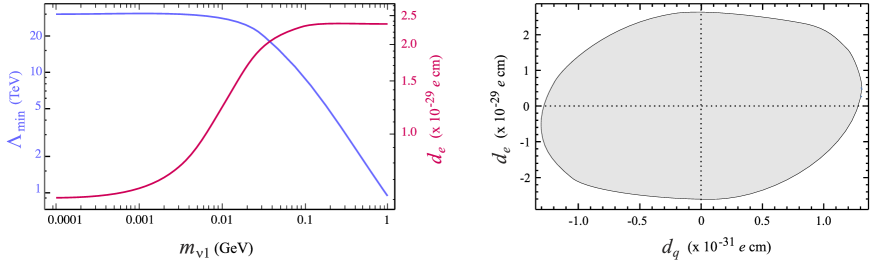
Figure 8: Left: The minimal scale $\Lambda$ of the magnetic operators, Eq. (1), and the corresponding electron EDM, such that $\mu\rightarrow e\gamma$ saturates its experimental limit when $M_{\Delta}/v\lambda_{\Delta}$ is set at the perturbativity bound, Eq. (98), as functions of the lightest neutrino mass $m_{\nu 1}$. Right: Range of accessible quark and lepton EDMs in the Type II seesaw, given the perturbativity bound $\mathbf{\Upsilon}_{\Delta}^{IJ}\lesssim 4\pi$ and the experimental limit on $\mathcal{B}(\mu\rightarrow e\gamma)$.

Our goal is to check how large the EDMs could be given these two limits. We assume the magnetic operators all arise at one loop, and thus include a factor $g^{2}/16\pi^{2}$ in the LFV and EDM amplitudes. Given that $\mu\rightarrow e\gamma$ is in $\left(M_{\Delta}/v\lambda_{\Delta}\right)^{4}/\Lambda^{4}$ while EDMs are in $\left(M_{\Delta}/v\lambda_{\Delta}\right)^{4}/\Lambda^{2}$, our strategy is first to fix $M_{\Delta}/v\lambda_{\Delta}$ by saturating the perturbativity bound, and then to find for this value the minimum scale $\Lambda_{\min}$ for which $\mu\rightarrow e\gamma$ is compatible with its experimental limit, see Fig. 8. The dependence of $\mu\rightarrow e\gamma$ on the $\mathcal{CP}$-violating phases is weak, so this lower bound on $\Lambda$ is rather strong. With these two inputs, $M_{\Delta}/v\lambda_{\Delta}$ and $\Lambda_{\min}$, we then compute the maximal quark and lepton EDMs by scanning over the three $\mathcal{CP}$-violating phases $\delta_{13}$, $\alpha_{M}$ and $\beta_{M}$. As explained in the previous section (see Fig. 7), the two types of EDMs are decorrelated and span quite uniformly the area shown in Fig. 8. Provided $\mathbf{\Upsilon}_{\Delta}^{IJ}\$can saturate its perturbativity bound, the electron EDM can get close to its experimental limit $|d_{e}|\,<8.7\cdot 10^{-29}\,e\cdot cm\;(90\%)$ [20]. In this respect, it should be stressed that the perturbativity bound really plays the crucial role. If one imposes $\mathbf{\Upsilon}_{\Delta}^{IJ}\lesssim 1$ instead of $\mathbf{\Upsilon}_{\Delta}^{IJ}\lesssim 4\pi$, the maximal value for $M_{\Delta}/v\lambda_{\Delta}$ gets reduced by $4\pi$, and so is $\Lambda_{\min}$ if the $\mu\rightarrow e\gamma$ bound remains saturated, but the electron EDM end up reduced by $(4\pi)^{2}\approx 160$.

Concerning the quarks, the situation is more involved than it seems. First, the $\mu\rightarrow e\gamma$ bound imply $|J_{\mathcal{CP}}^{\mathrm{Majo,2}}|_{\max}\approx 10^{-6}$. Naively, this pushes their EDMs from the magnetic operators beyond $10^{-31}$ $e\cdot cm$. But, at the same time, $J_{\mathcal{CP}}^{\mathrm{Majo,2}}$ also shift the $\theta$ term as

$$\Delta\theta_{eff}^{quarks}\sim\frac{g^{2}}{4\pi^{2}}\times J_{\mathcal{CP}}^{\mathrm{Majo,2}}\sim 10^{-8}\;.$$ (99)

Given the crude approximations involved, we consider this (barely) compatible with the bound $\theta_{C}^{eff}\lesssim 10^{-10}$. It shows that the neutron EDM induced by leptonic $\mathcal{CP}$-violating phases could in principle saturate its experimental limit.

The $\theta$ term shift brings tight constraints. Consider for example the Type II seesaw extended to allow for several Higgs doublets. The spurion background values are then tuned by different vacuum expectation values,

$$v_{d}\mathbf{Y}_{e}=\mathbf{m}_{e},\;\;\;v_{u}\mathbf{\Upsilon}_{\nu}\equiv v_{u}^{2}\mathbf{\Upsilon}_{\Delta}\frac{\lambda_{\Delta}}{M_{\Delta}}\equiv U_{PMNS}^{\ast}\mathbf{m}_{\nu}U_{PMNS}^{\dagger}\;.$$ (100)

Crucially, the spurion combinations relevant for the EDMs scale differently in the large $\tan\beta=v_{u}/v_{d}$ limit

$$J_{\mathcal{CP}}^{\mathrm{Majo,2}}\sim\left(\tan\beta\right)^{4}\;\;,\;\;\;(\mathbf{X}_{e}^{\mathrm{Majo,2}})^{11}\sim\left(\tan\beta\right)^{2}\;,$$ (101)

while the LFV rates are not directly affected. If $\tan\beta$ is large, the lightest neutrino mass and/or the $\mathcal{CP}$-violating phases must be such that $J_{\mathcal{CP}}^{\mathrm{Majo,2}}$ is far from its maximal value to satisfy the bound $\theta_{C}^{eff}\lesssim 10^{-10}$. At that point, it is quite possible that $d_{e}$ would be unobservably small, but $d_{n}$ close to its experimental bound. Alternatively, such a large shift $\Delta\theta_{eff}^{quarks}$ would be totally irrelevant if the mechanism solving the SM strong $\mathcal{CP}$ puzzle rotates the whole $\theta_{C}^{eff}$ away. Then, the EDM are again entirely induced by the magnetic operators, Eq. (1). As $J_{\mathcal{CP}}^{\mathrm{Majo,2}}$ increases faster with $\tan\beta$ than $(\mathbf{X}_{e}^{\mathrm{Majo,2}})^{11}$, we can even imagine that the current limit on the electron EDM is saturated by a pure $J_{\mathcal{CP}}^{\mathrm{Majo,2}}$. Given $|d_{e}|\,<8.7\cdot 10^{-29}\,e\cdot cm$, this corresponds to

$$|J_{\mathcal{CP}}^{\mathrm{Majo,2}}|_{\max}\approx 10^{-3}\times\left[\frac{\Lambda_{\min}}{1\,\text{TeV}}\right]^{2}\;,$$ (102)

to be compared to $|J_{\mathcal{CP}}^{\mathrm{Majo,2}}|_{\max}\approx 10^{-6}$ when $\tan\beta=1$. At this point, the bound Eq. (91) implies that the quark EDM cannot be over $d_{q}\approx 10^{-27}$ $e\cdot cm$, which thus represents the maximal attainable value in the absence of $\theta_{C}^{eff}$.

In conclusion, the Type II seesaw does not predict clear patterns between the LFV rates, quark and lepton EDM. A discovery could be around the corner for any one of them.

4.3.2 Type I and III Seesaw mechanisms

The Type I seesaw adds to the SM a flavor-triplet of right-handed neutrinos. The gauge interactions then allow for both a Dirac and a Majorana mass term

$$\mathcal{L}=\mathcal{L}_{SM}+i\bar{N}\!\not\!\partial N+\left(-\frac{1}{2}\bar{N}^{\mathrm{C}}\mathbf{M}N-\bar{N}^{\mathrm{C}}\mathbf{Y}_{\nu}LH+h.c.\right)\;.$$ (103)

Further, the Majorana mass term is a priori unrelated to the electroweak scale, and could well be much larger. Assuming $\mathbf{M}=\operatorname*{diag}(M_{1},M_{2},M_{3})$ without loss of generality and integrating out the $N$ fields, we get back the Weinberg operator

$$\mathcal{L}_{eff}=\mathcal{L}_{SM}+\frac{1}{2}(\bar{L}^{\mathrm{C}}H)\mathbf{Y}_{\nu}^{T}\mathbf{M}^{-1}\mathbf{Y}_{\nu}(LH)+h.c.\;.$$ (104)

Provided $\mathbf{M}$ is sufficiently large, the left-handed neutrino masses are tiny even with neutrino Yukawa couplings of natural size, $\mathbf{Y}_{\nu}\sim\mathcal{O}(\mathbf{Y}_{u,d,e})$.

Instead of a flavor triplet of weak singlets $N$, one could introduce flavor triplets of weak triplets $\Sigma_{i}$, $i=1,2,3$, with zero hypercharge. This is the Type III seesaw. Such fields can couple to weak doublets through their vector current as

$$\mathcal{L}=\mathcal{L}_{SM}+i\bar{\Sigma}_{i}\!\not\!D\Sigma_{i}+\left(-\frac{1}{2}\bar{\Sigma}_{i}^{\mathrm{C}}\mathbf{M}\Sigma_{i}-\bar{\Sigma}_{i}^{\mathrm{C}}\mathbf{Y}_{\nu}(L\sigma^{i}H)+h.c.\right)\;.$$ (105)

The fields $\Sigma_{i}$ being in the adjoint representation, the adequate couplings to gauge bosons are understood in the covariant derivative, and a gauge-invariant Majorana mass is allowed. Clearly, from a flavor symmetry point of view, the spurion content is identical to that of the Type I seesaw mechanism. Further, integrating out the $\Sigma_{i}$ fields produces exactly the same Weinberg operator as in Eq. (104). In the remainder of this section, we thus proceed with the Type I seesaw, but it should be clear that our developments equally apply to the Type III mechanism.

At the seesaw scale, we have two elementary flavor-breaking parameters $\mathbf{M}$ and $\mathbf{Y}_{\nu}$ which transform under the larger flavor-symmetry group $G_{F}^{\prime}\equiv G_{F}\times U(3)_{N}$ [49]. But since $\nu_{R}$ is not dynamical at low-energy, no amplitude ever transform non-trivially under $U(3)_{N}$. Only combinations of $\mathbf{Y}_{\nu}$ and $\mathbf{M}$ transforming as singlets under $U(3)_{N}$ are needed. Further, integrating out $\nu_{R}$ generates an inverse-mass expansion, and with $\mathbf{M}\sim 10^{10}-10^{13}$ GeV, only the leading spurion combinations need to be kept:

$$\mathbf{Y}_{e} \sim\left(\mathbf{\bar{3}},\mathbf{\bar{3}},\mathbf{1}\right)_{L,E,N}:\mathbf{Y}_{e}\overset{G_{F}}{\rightarrow}g_{E}^{\dagger}\mathbf{Y}_{e}g_{L}^{\dagger}\;,\;$$ (106a)

$$\mathbf{Y}_{\nu}^{\dagger}\mathbf{Y}_{\nu} \sim\left(\mathbf{8},\mathbf{1},\mathbf{1}\right)_{L,E,N}:\mathbf{Y}_{\nu}^{\dagger}\mathbf{Y}_{\nu}\overset{G_{F}}{\rightarrow}g_{L}\mathbf{Y}_{\nu}^{\dagger}\mathbf{Y}_{\nu}g_{L}^{\dagger}\;,$$ (106b)

$$\mathbf{\Upsilon}_{\nu}\overset{}{\equiv}v\mathbf{Y}_{\nu}^{T}(\mathbf{M}^{-1})\mathbf{Y}_{\nu} \sim\left(\mathbf{\bar{6}},\mathbf{1},\mathbf{1}\right)_{L,E,N}\;:\mathbf{\Upsilon}_{\nu}\overset{G_{F}}{\rightarrow}g_{L}^{\ast}\mathbf{\Upsilon}_{\nu}g_{L}^{\dagger}\;.$$ (106c)

The symmetric $$\mathbf{\Upsilon}_{\nu}^{T}=\mathbf{\Upsilon}_{\nu} \mathbf{Y}_{e},\mathbf{Y}_{\nu}^{\dagger}\mathbf{Y}_{\nu}\gg\mathbf{\Upsilon}_{\nu} SU(3)^{5}$$ corresponds to the very small Majorana mass term for the left-handed neutrinos. The scaling is stable since these spurion combinations live in different triality classes.

As is well known, it is not possible to unambiguously fix the background value of $\mathbf{Y}_{\nu}^{\dagger}\mathbf{Y}_{\nu}$ from the available neutrino data. Without loss of generality, this underdetermination can be parametrized [50] in terms of an unknown complex orthogonal matrix $\mathbf{R}$ as $v\mathbf{Y}_{\nu}=(\mathbf{M}^{1/2})\mathbf{R}(\mathbf{m}_{\nu}^{1/2})U_{PMNS}^{\dagger}$ where $U_{PMNS}^{\dagger}$ is defined from the diagonalization of $\mathbf{Y}_{e}$ and $\mathbf{\Upsilon}_{\nu}$ and contains Majorana phases, see Eq. (75). To proceed, we assumed that right-handed neutrinos are degenerate, at least in a good approximation [51]. This means that $\mathbf{M}$ does not break $U(3)_{N}$ entirely but leaves its $O(3)$ subgroup exact, and three parameters can be eliminated. Specifically, starting with the polar decomposition $\mathbf{R}=\mathbf{U\,H}$ with $\mathbf{U}=(\mathbf{R}^{\dagger}\mathbf{R})^{1/2}$ unitary and $\mathbf{H}=\mathbf{U}^{\dagger}\mathbf{R}$ hermitian, and imposing $\mathbf{R}^{T}\mathbf{R}=1$, the six-parameter orthogonal $\mathbf{R}$ matrix decomposes as $\mathbf{R}=\mathbf{O}\mathrm{\,}\mathbf{H}$ with $\mathbf{O}$ a real orthogonal matrix and $\mathbf{H}$ a hermitian orthogonal matrix. The degeneracy $\mathbf{M}=M_{R}\mathbf{1}$ permits to get rid of the former through the innocuous redefinition $N\rightarrow\mathbf{O}^{T}N$, so that $\mathbf{Y}_{\nu}^{\dagger}\mathbf{Y}_{\nu}$ simplifies to [52]

$$\mathbf{\mathbf{Y}}_{\nu}^{\dagger}\mathbf{\mathbf{Y}}_{\nu}=\frac{M_{R}}{v^{2}}U_{PMNS}(\mathbf{m}_{\nu}^{1/2})\,\mathbf{H}^{2}\mathbf{\,}(\mathbf{m}_{\nu}^{1/2})U_{PMNS}^{\dagger}\;,$$ (107)

with the matrix $\mathbf{H}$ written in terms of an antisymmetric real matrix $\mathbf{\Phi}^{IJ}=\varepsilon^{IJK}\phi_{K}$ as [52, 51]

$$\mathbf{H}=e^{i\mathbf{\Phi}}=\mathbf{1}+\frac{\cosh r-1}{r^{2}}i\mathbf{\Phi}\cdot i\mathbf{\Phi}+\frac{\sinh r}{r}i\mathbf{\Phi},\;\;r=\sqrt{\phi_{1}^{2}+\phi_{2}^{2}+\phi_{3}^{2}}\;.$$ (108)

The three real parameters $\phi_{1}$, $\phi_{2}$ and $\phi_{3}$ affect the size of the $\mathcal{CP}$-conserving entries in $\mathbf{\mathbf{Y}}_{\nu}^{\dagger}\mathbf{\mathbf{Y}}_{\nu}$ and induce $\mathcal{CP}$-violating imaginary parts.

In the absence of NP besides right-handed neutrinos, the LFV rates would arise only at $\mathcal{O}(\mathbf{M}^{-2})$,

$$\mathbf{X}_{e}^{\mathrm{Type\,I}}=\mathbf{Y}_{\nu}^{\dagger}\frac{v}{\mathbf{M}^{\dagger}}\frac{v}{\mathbf{M}}\mathbf{Y}_{\nu}+\mathbf{Y}_{\nu}^{\dagger}\frac{v}{\mathbf{M}^{\dagger}}\mathbf{Y}_{\nu}^{\ast}\mathbf{Y}_{\nu}^{T}\frac{v}{\mathbf{M}}\mathbf{Y}_{\nu}+...=\frac{v^{2}}{M_{R}^{2}}\mathbf{Y}_{\nu}^{\dagger}\mathbf{Y}_{\nu}+\mathbf{\Upsilon}_{\nu}^{\dagger}\mathbf{\Upsilon}_{\nu}+....$$ (109)

The second term reproduces exactly the pure Majorana case in Eq. (77) and leads to the rates quartic in neutrino masses, see Eq. (68). The first term gives quadratic rates instead, but is only slightly less suppressed (the same spurion combination tunes other FCNC operators, see e.g. Ref. [53]). The situation changes if some NP is present at an intermediate scale $\Lambda\ll M_{R}$. This dynamics could directly bring the sensitivity to $\mathbf{Y}_{\nu}$, so that

$$\mathbf{X}_{e}^{\mathrm{Type\,I}}=\mathbf{Y}_{\nu}^{\dagger}\mathbf{Y}_{\nu}\;.$$ (110)

Not only are the LFV rates quadratic in the neutrino masses instead of quartic, but they are enhanced by $M_{R}^{4}/\Lambda^{4}$ compared to the situation in Eq. (109). This typically occurs at one loop in supersymmetry, where the sparticle masses set the scale $\Lambda$ while slepton soft-breaking terms bring the $\mathbf{Y}_{\nu}^{\dagger}\mathbf{Y}_{\nu}$ dependence. Plugging this into the LFV rate, we derive from the experimental bound on $\mu\rightarrow e\gamma$,

$$|\mathbf{Y}_{\nu}^{\dagger}\mathbf{Y}_{\nu}|^{21}\lesssim(10^{-2}-10^{-4})\times\left[\frac{\Lambda}{1\,\text{TeV}}\right]^{2}\;,$$ (111)

depending on whether $c_{e}\approx g^{2}/16\pi^{2}$ or $c_{e}\approx 1$ in Eq. (60). This is very close to the perturbativity bound, $|\mathbf{Y}_{\nu}^{\dagger}\mathbf{Y}_{\nu}|\lesssim 4\pi$, which indirectly limits $M_{R}$ for given values of the light neutrino masses and $\phi_{i}$ parameters as

$$\dfrac{m_{\nu}^{\max}}{1\text{\thinspace eV}}\frac{M_{R}}{10^{13}\,\text{GeV}}\lesssim 12\pi e^{-2\sqrt{3}\max\phi_{i}}\;.$$ (112)

Because of the exponential dependences on the $\phi_{i}$, the seesaw scale has to quickly decrease when $\phi_{i}$ is above unity.

Turning to the EDMs, the two spurion combinations not suppressed by the seesaw scale are $\mathbf{Y}_{e}$ and $\mathbf{Y}_{\nu}^{\dagger}\mathbf{Y}_{\nu}$, out of which we can construct only:

$$J_{\mathcal{CP}}^{\mathrm{Type\,I}} =\frac{1}{2i}\det[\mathbf{Y}_{\nu}^{\dagger}\mathbf{Y}_{\nu},\mathbf{Y}_{e}^{\dagger}\mathbf{Y}_{e}]\;,$$ (113)

$$\mathbf{X}_{e}^{\mathrm{Type\,I}} =[\mathbf{Y}_{\nu}^{\dagger}\mathbf{Y}_{\nu}\;,\;\mathbf{Y}_{\nu}^{\dagger}\mathbf{Y}_{\nu}\mathbf{Y}_{e}^{\dagger}\mathbf{Y}_{e}\mathbf{Y}_{\nu}^{\dagger}\mathbf{Y}_{\nu}]\;.$$ (114)

From a symmetry point of view, those are the same as in the Dirac neutrino mass case, Eqs. (69) and (70). Beyond that superficial similarity, the situation is quite different as $\mathbf{Y}_{\nu}^{\dagger}\mathbf{Y}_{\nu}$ has far more degrees of freedom, and depends only linearly on the light neutrino masses. For instance, when $\phi_{i}=0$, we find $v^{2}(\mathbf{\mathbf{Y}}_{\nu}^{\dagger}\mathbf{\mathbf{Y}}_{\nu})^{\mathrm{Type\,I}}\rightarrow M_{R}U_{PMNS}\mathbf{m}_{\nu}U_{PMNS}^{\dagger}$ to be compared to $v^{2}(\mathbf{\mathbf{Y}}_{\nu}^{\dagger}\mathbf{\mathbf{Y}}_{\nu})^{\mathrm{Dirac}}\rightarrow U_{PMNS}\mathbf{m}_{\nu}^{2}U_{PMNS}^{\dagger}$ in the Dirac case. In other words, $J_{\mathcal{CP}}^{\mathrm{Type\,I}}$ and $\mathbf{X}_{e}^{\mathrm{Type\,I}}$ depend linearly on the product of the three neutrino mass differences in that limit, and are insensitive to Majorana phases. On the contrary, both these features are lost as soon as $\phi_{i}\neq 0$: neither $J_{\mathcal{CP}}^{\mathrm{Type\,I}}$ nor $\mathbf{X}_{e}^{\mathrm{Type\,I}}$ vanish when only two neutrinos are degenerate, and both are sensitive to the Majorana phases. What is preserved though is their dependence on the charged lepton masses,

$$J_{\mathcal{CP}}^{\mathrm{Type\,I}}\sim\prod_{i>j=e,\mu,\tau}\frac{m_{i}^{2}-m_{j}^{2}}{v^{2}}\;,\;\;(\mathbf{X}_{e}^{\mathrm{Type\,I}})^{11}\sim\frac{m_{\tau}^{2}-m_{\mu}^{2}}{v^{2}}\;.$$ (115)

Remarkably, these charged lepton mass differences are multiplied by the same factor for both expressions, even when $\phi_{i}\neq 0$. This means that contrary to the Majorana case (see Figs. 7 and 8), the ratio is fixed at

$$\frac{\operatorname{Im}(\mathbf{X}_{e}^{\mathrm{Type\,I}})^{11}}{2J_{\mathcal{CP}}^{\mathrm{Type\,I}}}=\frac{\operatorname{Im}(\mathbf{X}_{e}^{\mathrm{Dirac}})^{11}}{2J_{\mathcal{CP}}^{\mathrm{Dirac}}}=\frac{v^{4}}{(m_{\tau}^{2}-m_{e}^{2})(m_{\mu}^{2}-m_{e}^{2})}\approx 10^{11}\;\rightarrow\frac{d_{q}}{m_{q}}\approx 10^{-11}\times\frac{d_{e}}{m_{e}}\;.$$ (116)

In stark difference to the Type II seesaw, the flavored contributions to the lepton and quark EDMs are strictly correlated in the Type I and III seesaw, and the latter remains much smaller than the former. Of course, dynamical effects can alter this strict correlation, for example through logarithmic dependences on the charged lepton mass. But nevertheless, the relative orders of magnitude of the lepton and quark EDM should be well predicted by the behavior of these spurion combinations.

An immediate consequence of the suppression of $J_{\mathcal{CP}}^{\mathrm{Type\,I}}$ is that of the quark EDMs. Both the magnetic contributions and that generated by a shift of the $\theta$ term are tuned by $J_{\mathcal{CP}}^{\mathrm{Type\,I}}$, which is at least 11 orders of magnitude smaller than $(\mathbf{X}_{e}^{\mathrm{Type\,I}})^{11}$. The neutron EDM thus remain entirely dominated by CKM contributions, whatever happens in the leptonic sector. This conclusion remains true in the presence of two Higgs doublets, since Eq. (116) is modified to

$$\frac{\operatorname{Im}(\mathbf{X}_{e}^{\mathrm{Type\,I}})^{11}}{2J_{\mathcal{CP}}^{\mathrm{Type\,I}}}\approx\frac{v^{4}}{(m_{\tau}^{2}-m_{e}^{2})(m_{\mu}^{2}-m_{e}^{2})}\frac{1}{(\tan\beta)^{4}}\approx 10^{5}\times\left(\frac{50}{\tan\beta}\right)^{4}\;.$$ (117)

With such a large hierarchy, the current limit from $d_{e}$ excludes any signal in $d_{q}$.

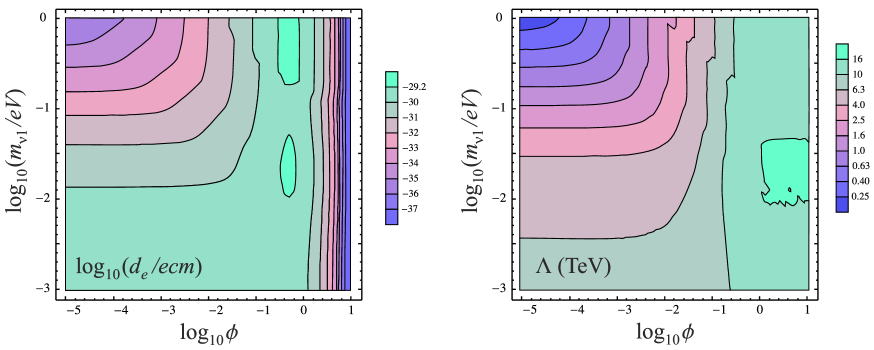
Figure 9: Electron EDM and minimal effective operator scale $\Lambda_{\min}$ at which $\mu\rightarrow e\gamma$ is compatible with its experimental limit, as a function of the lightest neutrino mass and $\phi=\phi_{1}=\phi_{2}=\phi_{3}$ parameter. Implicitly, the seesaw scale is set for each input values of these parameters by saturating the perturbativity bound, $|\mathbf{Y}_{\nu}^{\dagger}\mathbf{Y}_{\nu}|\lesssim 4\pi$, while EDM is maximized over the three $\mathcal{CP}$-violating phases (at which stage numerical fluctuations can arise, hence the small irregularities in the contours).

The situation for the lepton EDMs is different. To find the maximal attainable values (with $\tan\beta=1$), let us follow the same strategy as for the Type II seesaw, with here $\mu\rightarrow e\gamma$ behaving as $M_{R}^{2}/\Lambda^{4}$ and EDMs as $M_{R}^{3}/\Lambda^{2}$. So, for given lightest neutrino mass $m_{\nu 1}$, parameter $\phi\equiv\phi_{1}=\phi_{2}=\phi_{3}$, and $\mathcal{CP}$-violating phases, we adjust $M_{R}$ to saturate the perturbativity bound $|\mathbf{Y}_{\nu}^{\dagger}\mathbf{Y}_{\nu}|\lesssim 4\pi$. Then, we find the minimal scale $\Lambda_{\min}$ for which $\mu\rightarrow e\gamma$ is compatible with its experimental limit, and compute the EDMs assuming they arise at the same scale. Also, to maintain the parallel with the seesaw Type II discussed before, we include a factor $g^{2}/16\pi^{2}$ for all the magnetic operators. The result of this analysis is shown in Fig. 9. As in the Type II seesaw, it is possible to bring $d_{e}$ close to its experimental limit provided the perturbativity bound is enforced as $|\mathbf{Y}_{\nu}^{\dagger}\mathbf{Y}_{\nu}|\lesssim 4\pi$. Asking for $|\mathbf{Y}_{\nu}^{\dagger}\mathbf{Y}_{\nu}|\lesssim 1$ reduces $M_{R}$ by $4\pi$ but increases $\Lambda_{\min}$ by $\sqrt{4\pi}$, for a net reduction of all the EDMs by two orders of magnitude, $(4\pi)^{2}\approx 160$. In that case, increasing $\tan\beta$ is necessary to bring back $d_{e}$ above $10^{-30}$ $e\cdot cm$.

4.4 Majorana mass terms and anomalous invariants

The Majorana mass term explicitly violates lepton number, which is nothing but a specific linear combination of the five flavor $U(1)$s of the flavor group $U(3)^{5}$. As in the quark sector, this means invariants under $SU(3)^{5}$ should be considered. Specifically, generalizing Eq. (75) to $U_{PMNS}=U_{PMNS}^{\mathrm{Dirac}}\cdot\operatorname{diag}(e^{i\gamma_{M}},e^{i\alpha_{M}},e^{i\beta_{M}})$, the leptonic structures invariant under $SU(3)^{5}$ but not $U(3)^{5}$ necessarily involve

$$\operatorname{Im}\det\mathbf{\Upsilon}_{\nu} =\frac{m_{\nu 1}m_{\nu 2}m_{\nu 3}}{v^{3}}\sin(\alpha_{M}+\beta_{M}+\gamma_{M})\;,$$ (118)

$$\operatorname{Im}\varepsilon^{AJL}\varepsilon^{IKM}\mathbf{\Upsilon}_{\nu}^{IJ}\mathbf{\Upsilon}_{\nu}^{KL}\mathbf{\Upsilon}_{\nu}^{MB} =\operatorname{Im}\det\mathbf{\Upsilon}_{\nu}\varepsilon^{AJL}\varepsilon^{BJL}=2\delta^{AB}\operatorname{Im}\det\mathbf{\Upsilon}_{\nu}\;.$$ (119)

With neutrino masses of around $0.1$ eV, these structures are both $\mathcal{O}(10^{-34})$, i.e., much larger than those invariant under the full $U(3)^{5}$. Further, in a Type II seesaw, one would expect $\operatorname{Im}\det\mathbf{\Upsilon}_{\Delta}$ to appear instead, which could reach up to $\mathcal{O}(1)$ values. The question we want to address here is whether those actually contribute to physical observables like EDMs or can be rotated away.

4.4.1 Electroweak anomalous interactions

As a first step, the interplay between the Majorana mass term and the $\mathcal{CP}$-violating $\theta_{W}W_{\mu\nu}\tilde{W}^{\mu\nu}$ coupling of the SM must be identified. Specifically, under flavored $U(1)$ transformations with parameters $3\alpha_{Q,L}=\arg\det V_{L}^{d,e\dagger}$ and $3\alpha_{U,D,E}=\arg\det V_{R}^{u,d,e}$,

$$\theta_{W}\rightarrow\theta_{W}^{eff}=\theta_{W}-3\left(\alpha_{L}+3\alpha_{Q}\right)\;.$$ (120)

In the SM, because $U(1)_{\mathcal{B}+\mathcal{L}}$ is anomalous, it is always possible to choose $\alpha_{L}+3\alpha_{Q}$ so as to set $\theta_{W}^{eff}=0$ since both $\alpha_{L}$ and $\alpha_{Q}$ are left free once the three conditions in Eq. (35) are enforced. This does not separately fix $\alpha_{L}$ and $\alpha_{Q}$ because $U(1)_{\mathcal{B}-\mathcal{L}}$ remains as an exact non-anomalous symmetry. In the presence of a Majorana mass term, both $U(1)_{\mathcal{B}+\mathcal{L}}$ and $U(1)_{\mathcal{B}-\mathcal{L}}$ are broken explicitly, and all the $U(1)$ rotations are fixed. Indeed, the phase convention for the Majorana phases determines $\alpha_{L}$ since in addition to the three conditions Eq. (35), there is now

$$\arg\det\mathbf{\Upsilon}_{\nu}=2\arg\det U_{PMNS}^{\dagger}+2\arg\det V_{L}^{e\dagger}=-2(\alpha_{M}+\beta_{M}+\gamma_{M})+6\alpha_{L}\;.$$ (121)

Once $\alpha_{L}$ is chosen to eliminate $\gamma_{M}$ say, $\alpha_{Q}$ has to be adjusted accordingly to cancel $\theta_{W}^{eff}$, while $\alpha_{U,D,E}$ are fixed by the requirement of real fermion masses, Eq. (35). The main consequence of all this is that the phase of the simple invariant $\det\mathbf{\Upsilon}_{\nu}$ cannot be physical since it is always possible to choose $\alpha_{L}=(\alpha_{M}+\beta_{M}+\gamma_{M})/3$, in which case $\arg\det\mathbf{\Upsilon}_{\nu}=0$. Note that this also explains a posteriori our choice in Eq. (39). It is compulsory to account for $\theta_{C}^{eff}$ by acting only on right-handed weak singlet fields, since otherwise $\alpha_{Q}$ would not be free but depend on $\theta_{C}^{eff}$. In turn, $\alpha_{L}$ would have to be fixed in terms of $\theta_{C}^{eff}$ to eliminate $\theta_{W}$, and the neutrino Majorana phases would end up depending on $\theta_{C}^{eff}$.

The reality of $\det\mathbf{\Upsilon}_{\nu}$ rests on the possibility to choose $\alpha_{L}$ even after $\theta_{W}$ has been rotated away. Because the whole Lagrangian but the $\mathbf{\Upsilon}_{\nu}$ term is invariant under $U(1)_{\mathcal{B}-\mathcal{L}}$, this symmetry can be used to get rid of the global phase of the Majorana mass term. The natural question to ask at this stage is what happens if other interactions beside $\mathbf{\Upsilon}_{\nu}$ violate $\mathcal{B}$ and/or $\mathcal{L}$. Clearly, the electroweak $\mathcal{B}+\mathcal{L}$ anomalous interactions

$$\mathcal{L}_{SM}^{\mathcal{B}+\mathcal{L}}\sim g_{SM}^{\mathcal{B}+\mathcal{L}}(\varepsilon^{IJK}Q^{I}Q^{J}Q^{K})^{3}\times(\varepsilon^{IJK}L^{I}L^{J}L^{K})\;,$$ (122)

is unaffected by the phase convention adopted for the Majorana phases since it transforms as

$$g_{SM}^{\mathcal{B}+\mathcal{L}}\rightarrow g_{SM}^{\mathcal{B}+\mathcal{L}}\exp 3i(3\alpha_{Q}+\alpha_{L})=g_{SM}^{\mathcal{B}+\mathcal{L}}\exp 3i\theta_{W}\;,$$ (123)

when $\theta_{W}^{eff}=0$. Because the same $3\alpha_{Q}+\alpha_{L}$ combination as in Eq. (120) appears, this phase is unequivocally fixed once requiring the absence of the $W_{\mu\nu}\tilde{W}^{\mu\nu}$ term [54]. The same is true for the dimension-six Weinberg operators [40], since they also preserve $\mathcal{B}-\mathcal{L}$.

4.4.2 Majorana invariants from $\mathcal{B}$ and $\mathcal{L}$ violating couplings

It is only in the presence of $\mathcal{B}$ and/or $\mathcal{L}$ violating couplings not aligned with either the Majorana mass ($\Delta\mathcal{L}=2n$, integer $n$) or the $\mathcal{B}+\mathcal{L}$ anomalous coupling that their phases cannot be defined unambiguously. To illustrate this, consider the two dimension-nine operators (here written in terms of left-handed Weyl spinors) [55]

$$\mathcal{H}_{eff}=\delta_{1}\frac{EL^{2}U^{3}}{\Lambda^{5}}+\delta_{2}\frac{U^{2}D^{4}}{\Lambda^{5}}+h.c.\;,$$ (124)

where $\delta_{1}$ induce $\Delta\mathcal{L}=3,\Delta\mathcal{B}=1$ transitions, and $\delta_{2}$ induce $\Delta\mathcal{L}=0,\Delta\mathcal{B}=2$ transitions. Under the $U(1)^{5}$ transformation,

$$\delta_{1} \rightarrow\delta_{1}\exp i(-\alpha_{E}+2\alpha_{L}-3\alpha_{U})\rightarrow\delta_{1}\exp i(3(\alpha_{L}+\alpha_{Q})-\frac{1}{3}\arg\det\mathbf{Y}_{e}-\arg\det\mathbf{Y}_{u})\;,$$ (125a)

$$\delta_{2} \rightarrow\delta_{2}\exp i(-2\alpha_{U}-4\alpha_{D})\rightarrow\delta_{2}\exp i(6\alpha_{Q}-\frac{2}{3}\arg\det\mathbf{Y}_{u}-\frac{4}{3}\arg\det\mathbf{Y}_{d})\;,$$ (125b)

where we have imposed Eq. (35). Because the two $$\mathcal{H}_{eff} \Delta\mathcal{B} \Delta\mathcal{L} U(1) \alpha_{L} \alpha_{Q} \mathcal{CP} \mathcal{CP} G_{a,\mu\nu}\tilde{G}^{a,\mu\nu} \mathcal{B} \mathcal{L} \mathcal{CP}$$ operators induce different and patterns as the neutrino Majorana mass or the SM anomalous couplings, they depend differently on the rotations. A given choice for and can remove violation from some couplings, but not all can be real simultaneously. This looks strikingly similar to the way the strong phase can be moved back and forth between the term and the quark mass terms, except that the physical contents of the various couplings is very different here. Having different and charges, they do not induce the same types of observables, so it is actually rather puzzling to be able to move a -violating phase around in this way.

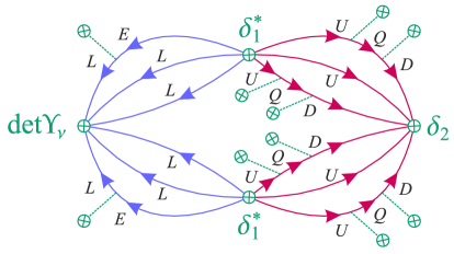
Figure 10: Diagrammatic representation of the EDM contribution arising from the combination of the effective couplings in Eq. (126a), where the tadpoles represent Yukawa coupling insertions.

The key to solve this is to assume that the invariant $\det\mathbf{\Upsilon}_{\nu}$ can only arise from an interaction carrying a global $\mathcal{L}=6$ charge. Whether local or not, this interaction then never contributes directly to the EDMs. Instead, at least two other misaligned $\mathcal{B}$ and/or $\mathcal{L}$ violating interactions are required to construct an overall $\Delta\mathcal{B}=\Delta\mathcal{L}=0$ combinations. At that stage, only the phase differences between the involved couplings matter, and those do not depend on the specific choices made for $\alpha_{L}$ and $\alpha_{Q}$. For example, in the presence of the dimension-nine and anomalous operators, the $\mathcal{CP}$-violating phases potentially inducing EDMs can arise from

$$\arg(\det\mathbf{\Upsilon}_{\nu}\cdot\delta_{1}^{\ast 2}\cdot\delta_{2})-\frac{2}{3}\arg\det\mathbf{Y}_{e}-\frac{4}{3}\arg\det\mathbf{Y}_{u}+\frac{4}{3}\arg\det\mathbf{Y}_{d} =-2(\alpha_{M}+\beta_{M}+\gamma_{M})\;,$$ (126a)

$$\arg(\det\mathbf{\Upsilon}_{\nu}\cdot\delta_{1}^{\ast 3}\cdot g_{SM}^{\mathcal{B}+\mathcal{L}})-\arg\det\mathbf{Y}_{e}-3\arg\det\mathbf{Y}_{u} =-2(\alpha_{M}+\beta_{M}+\gamma_{M})\;,$$ (126b)

$$\arg(\det\mathbf{\Upsilon}_{\nu}\cdot\delta_{2}^{3}\cdot(g_{SM}^{\mathcal{B}+\mathcal{L}})^{\ast 2})+2\arg\det\mathbf{Y}_{u}+4\arg\det\mathbf{Y}_{d} =-2(\alpha_{M}+\beta_{M}+\gamma_{M})\;,$$ (126c)

where $$\delta_{1,2} g_{SM}^{\mathcal{B}+\mathcal{L}} U(1)^{5} \operatorname{Im}\delta_{1,2}=0 \alpha \arg\det\mathbf{Y}_{u,d,e} U(1)^{5} \alpha_{U,D,E} \mathcal{CP} \Delta\mathcal{B} \Delta\mathcal{L} \delta_{1}^{2} \mathcal{CP} \delta_{2}\det\mathbf{\Upsilon}_{\nu}$$ and are assumed real, up to the rotations (that is, on the right-hand side of Eq. (125)). The three original Majorana phases appear in the same combination for all three mechanisms, independently of the choice of any of the ’s since they cancel out. The various terms appear because some flavor transitions are required to glue together the effective interactions, see Fig. 10. Altogether, the left-hand-side of these equations are invariant under the whole group. Under this form, it is thus clear that a different choice of in which the -violating phases are moved onto the fermion masses does not change the EDMs. Finally, note that once the presence of the and interactions makes the Majorana phase combination physical, it could also be accessed from other processes. Consider for example di-proton decay, as induced by a interaction. The phase of this amplitude is accessible only through interference with another amplitude, but all that is available is . The difference in phases of these two amplitudes is precisely that given in Eq. (126).

In practice, the existence of this additional contribution to the EDM is of no concern if $\operatorname{Im}\det\mathbf{\Upsilon}_{\nu}\lesssim\mathcal{O}(10^{-34})$. Even in the most favorable case that $\mathbf{\Upsilon}_{\Delta}\approx 10^{12}\times\mathbf{\Upsilon}_{\nu}$, the $\delta_{1}^{\ast 2}\delta_{2}$ factor brings a prohibitive $\Lambda^{-15}$ suppression so that

$$d_{e}\approx e\frac{m_{e}}{M_{W}^{2}}\frac{M_{W}^{15}}{\Lambda^{15}}\operatorname{Im}(\det\mathbf{\Upsilon}_{\Delta}\cdot\delta_{1}^{\ast 2}\cdot\delta_{2})\lesssim 10^{-37}\times\left[\frac{1\,\text{TeV}}{\Lambda}\right]^{15}\;e\cdot cm\;,$$ (127)

when $\operatorname{Im}(\det\mathbf{\Upsilon}_{\Delta}\cdot\delta_{1}^{\ast 2}\cdot\delta_{2})$ is of $\mathcal{O}(1)$. Alternatively, the currend limit on $d_{e}$ requires $\Lambda\gtrsim 250$ GeV. Since proton decay or neutron-antineutron oscillations should push $\Lambda$ above the TeV, even assuming MFV holds for these operators [55], this contribution is too small to be seen. Though the situation described here is rather peculiar, with effective operators of large dimensions only, this conclusion should be quite robust. Anyway, to stay on the safe side, it is worth to keep this mechanism in mind whenever neutrinos have Majorana mass terms and some interactions also happen to violate $\mathcal{B}$ and/or $\mathcal{L}$.

5 Conclusions

In this paper, the flavor structure of the EDMs in the SM and beyond was systematically analyzed by relying on tools and techniques inspired from Minimal Flavor Violation. It is customary to estimate the EDM, or more generally the size of $\mathcal{CP}$-violation, using Jarlskog-like invariants. However, this is valid only for processes in which $\mathcal{CP}$ violation occurs in a closed fermion loop. For the CKM contributions to the quark EDM, or the PMNS contributions to lepton EDMs, the dominant diagrams have a rainbow topology whose flavor structure does not collapse to flavor invariants. The flavor symmetry is well suited to study these diagrams, and with the help of Cayley-Hamilton identities, permits to identify their flavor structures. In addition, the combined study of both Jarlskog-like and rainbow-like flavor structures shed new lights on the possible correlations between quark and lepton EDM. Interestingly, we find opposite behavior for Dirac or Majorana neutrinos. Quark and lepton EDM are strictly proportional in the former case, but becomes largely independent in the latter situation. As a consequence, the quark EDM is necessarily beyond our reach in the Type I seesaw because all the large flavor structures are of the Dirac type. On the contrary, the quark EDMs could be our best window into the Type II seesaw because the enhanced neutrino flavor structure is of the Majorana type.

Throughout this paper, special care was devoted to flavor-singlet $\mathcal{CP}$-violating phases. Those associated to the $U(1)$ subgroups of the flavor symmetry group, of which several combinations happen to be anomalous in the SM. The flavor symmetry was adapted to deal with this type of phases, by keeping track of them in the background values of the Yukawa couplings or Majorana mass terms. This permits to parametrize the impact of the strong $\mathcal{CP}$-violating interaction on both quark and lepton EDMs, or to analyze the interplay between the Majorana phases and possible baryon and/or lepton number violating interactions.

The techniques developed in this paper can easily be adapted to more complicated settings, for example in the presence of more than three light neutrino states, or with additional flavor structures not aligned with those of the minimal seesaw mechanisms. In these contexts, it is important to consider not only the Jarlskog-like invariants but also the non-invariant flavor structures. Being in general far less suppressed, they are of paramount phenomenological importance, and often represent our only window into the underlying physics.

Appendix A Cayley-Hamilton Theorem

The Cayley-Hamilton Theorem states that any $n\times n$ square matrix $\mathbf{X}$ is solution of its own characteristic equation, once extrapolated to matrix form

$$p\left(\lambda\right)=\det\left[\mathbf{X}-\lambda\mathbf{1}\right]\Rightarrow p\left(\mathbf{X}\right)=\mathbf{0}\;.$$ (128)

Specializing to $3\times 3$ hermitian matrices, the three eigenvalues $\lambda_{1,2,3}$ of $\mathbf{X}$ can be expressed back in terms of traces and determinant of $\mathbf{X}$, hence:

$$p\left(\mathbf{X}\right)=\left(\mathbf{X}-\lambda_{1}\mathbf{1}\right)\left(\mathbf{X}-\lambda_{2}\mathbf{1}\right)\left(\mathbf{X}-\lambda_{3}\mathbf{1}\right)=\mathbf{X}^{3}-\langle\mathbf{X}\rangle\mathbf{X}^{2}+\dfrac{1}{2}\mathbf{X}(\langle\mathbf{X}\rangle^{2}-\langle\mathbf{X}^{2}\rangle)-\det\mathbf{X}=0\;.$$ (129)

Taking the trace of this equation, $\det\mathbf{X}$ can be eliminated as

$$\det\mathbf{X}=\frac{1}{3}\langle\mathbf{X}^{3}\rangle-\frac{1}{2}\langle\mathbf{X}\rangle\langle\mathbf{X}^{2}\rangle+\dfrac{1}{6}\langle\mathbf{X}\rangle^{3}\;.$$ (130)

Additional identities can be derived by expressing $\mathbf{X}=x_{1}\mathbf{X}_{1}+x_{2}\mathbf{X}_{2}+...$ and extracting a given power of $x_{1}$, $x_{2}$,$...$.

References

• [1] G. D’Ambrosio, G. F. Giudice, G. Isidori and A. Strumia, Nucl. Phys. B 645 (2002) 155 [hep-ph/0207036].
• [2] C. Jarlskog, Phys. Rev. Lett. 55 (1985) 1039.
• [3] E. P. Shabalin, Sov. Phys. Usp. 26 (1983) 297 [Usp. Fiz. Nauk 139 (1983) 561].
• [4] I. B. Khriplovich, Phys. Lett. B 173 (1986) 193 [Sov. J. Nucl. Phys. 44 (1986) 659] [Yad. Fiz. 44 (1986) 1019].
• [5] A. Czarnecki and B. Krause, Phys. Rev. Lett. 78 (1997) 4339 [hep-ph/9704355].
• [6] G. C. Branco, R. G. Felipe and F. R. Joaquim, Rev. Mod. Phys. 84 (2012) 515 [arXiv:1111.5332 [hep-ph]].
• [7] C. Smith, Minimal Flavor Violation, Habilitation thesis, Université Grenoble Alpes, 2015.
• [8] J.-M. Gérard, Z. Phys. C 18 (1983) 145; R. S. Chivukula and H. Georgi, Phys. Lett. B 188 (1987) 99.
• [9] S. L. Glashow, J. Iliopoulos and L. Maiani, Phys. Rev. D 2 (1970) 1285.
• [10] A. J. Buras, in Les Houches 1997, Probing the standard model of particle interactions, F. David and R. Gupta (eds.), 1998, Elsevier Science B.V., hep-ph/9806471.
• [11] T. Inami and C. S. Lim, Prog. Theor. Phys. 65 (1981) 297 [Erratum-ibid. 65 (1981) 1772].
• [12] M. Pospelov and A. Ritz, Annals Phys. 318 (2005) 119 [hep-ph/0504231].
• [13] M. Raidal et al., Eur. Phys. J. C 57 (2008) 13 [arXiv:0801.1826 [hep-ph]].
• [14] J. P. Miller, E. de Rafael and B. L. Roberts, Rept. Prog. Phys. 70 (2007) 795 [hep-ph/0703049].
• [15] L. Mercolli and C. Smith, Nucl. Phys. B 817 (2009) 1 [arXiv:0902.1949 [hep-ph]].
• [16] C. Patrignani et al. [Particle Data Group], Chin. Phys. C 40 (2016) no.10, 100001. doi:10.1088/1674-1137/40/10/100001
• [17] J. F. Donoghue, Phys. Rev. D 18 (1978) 1632.
• [18] E. P. Shabalin, Sov. J. Nucl. Phys. 28 (1978) 75 [Yad. Fiz. 28 (1978) 151]; M. J. Booth, hep-ph/9301293; A. Czarnecki and B. Krause, Acta Phys. Polon. B 28 (1997) 829 [hep-ph/9611299].
• [19] M. Pospelov and A. Ritz, Phys. Rev. D 89 (2014) 5, 056006 [arXiv:1311.5537 [hep-ph]].
• [20] J. Baron et al. [ACME Collaboration], Science 343 (2014) 269 [arXiv:1310.7534 [physics.atom-ph]].
• [21] G. W. Bennett et al. [Muon (g-2) Collaboration], Phys. Rev. D 80 (2009) 052008 [arXiv:0811.1207 [hep-ex]].
• [22] K. Inami et al. [Belle Collaboration], Phys. Lett. B 551 (2003) 16 [hep-ex/0210066].
• [23] M. E. Pospelov, Phys. Lett. B 328 (1994) 441 [hep-ph/9402317].
• [24] G. Colangelo, E. Nikolidakis and C. Smith, Eur. Phys. J. C 59 (2009) 75 [arXiv:0807.0801 [hep-ph]].
• [25] C. Smith, JHEP 1705 (2017) 018 [arXiv:1612.03825 [hep-ph]].
• [26] A. Romanino and A. Strumia, Nucl. Phys. B 490 (1997) 3 [hep-ph/9610485].
• [27] I. B. Khriplovich and A. R. Zhitnitsky, Phys. Lett. B 109 (1982) 490.
• [28] C. A. Baker et al., Phys. Rev. Lett. 97 (2006) 131801 [hep-ex/0602020].
• [29] E. Nikolidakis and C. Smith, Phys. Rev. D 77 (2008) 015021 [arXiv:0710.3129 [hep-ph]].
• [30] G. ’t Hooft, Phys. Rev. Lett. 37 (1976) 8; Phys. Rev. D 14 (1976) 3432 [Erratum-ibid. D 18 (1978) 2199].
• [31] H. Y. Cheng, Phys. Rept. 158 (1988) 1.
• [32] I. B. Khriplovich and A. I. Vainshtein, Nucl. Phys. B 414 (1994) 27 [hep-ph/9308334].
• [33] J. R. Ellis and M. K. Gaillard, Nucl. Phys. B 150 (1979) 141.
• [34] J. M. Gérard and P. Mertens, Phys. Lett. B 716 (2012) 316 [arXiv:1206.0914 [hep-ph]].
• [35] Z. Maki, M. Nakagawa and S. Sakata, Prog. Theor. Phys. 28 (1962) 870; B. Pontecorvo, Sov. Phys. JETP 26, 984 (1968) [Zh. Eksp. Teor. Fiz. 53, 1717 (1967)].
• [36] I. Esteban, M. C. Gonzalez-Garcia, M. Maltoni, I. Martinez-Soler and T. Schwetz, JHEP 1701 (2017) 087 [arXiv:1611.01514 [hep-ph]].
• [37] J. Adam et al. [MEG Collaboration], Phys. Rev. Lett. 110 (2013) 201801 [arXiv:1303.0754 [hep-ex]].
• [38] B. Aubert et al. [BaBar Collaboration], Phys. Rev. Lett. 104 (2010) 021802 [arXiv:0908.2381 [hep-ex]].
• [39] S. A. Abel, A. Dedes and H. K. Dreiner, JHEP 0005 (2000) 013 [hep-ph/9912429].
• [40] S. Weinberg, Phys. Rev. Lett. 43 (1979) 1566.
• [41] G. C. Branco, L. Lavoura and M. N. Rebelo, Phys. Lett. B 180 (1986) 264.
• [42] G. C. Branco, M. N. Rebelo and J. I. Silva-Marcos, Phys. Rev. Lett. 82 (1999) 683 [hep-ph/9810328].
• [43] D. Ng and J. N. Ng, Mod. Phys. Lett. A 11 (1996) 211 [hep-ph/9510306]; A. de Gouvea and S. Gopalakrishna, Phys. Rev. D 72 (2005) 093008 [hep-ph/0508148]; Y. Liao, Phys. Lett. B 672 (2009) 367 [arXiv:0812.4324 [hep-ph]].
• [44] J. P. Archambault, A. Czarnecki and M. Pospelov, Phys. Rev. D 70 (2004) 073006 [hep-ph/0406089].
• [45] E. Ma, Phys. Rev. Lett. 81 (1998) 1171 doi:10.1103/PhysRevLett.81.1171 [hep-ph/9805219].
• [46] P. Minkowski, Phys. Lett. B 67 (1977) 421; M. Gell-Mann, P. Ramond, R. Slansky, proc. of the Supergravity Stony Brook Workshop, New York, 1979; T. Yanagida, proc. of the Workshop on the Baryon Number of the Universe and Unified Theories, Tsukuba, Japan, 1979; S. L. Glashow, Quarks and Leptons, Cargèse, 1979; R. N. Mohapatra and G. Senjanovic, Phys. Rev. D 23 (1981) 165.
• [47] G. B. Gelmini and M. Roncadelli, Phys. Lett. B 99 (1981) 411.
• [48] E. Ma and U. Sarkar, Phys. Rev. Lett. 80 (1998) 5716 [hep-ph/9802445].
• [49] V. Cirigliano, B. Grinstein, G. Isidori and M. B. Wise, Nucl. Phys. B 728 (2005) 121 [hep-ph/0507001].
• [50] J. A. Casas and A. Ibarra, Nucl. Phys. B 618 (2001) 171 [hep-ph/0103065].
• [51] V. Cirigliano, G. Isidori and V. Porretti, Nucl. Phys. B 763 (2007) 228 [hep-ph/0607068].
• [52] S. Pascoli, S. T. Petcov and C. E. Yaguna, Phys. Lett. B 564 (2003) 241 [hep-ph/0301095].
• [53] A. Broncano, M. B. Gavela and E. E. Jenkins, Phys. Lett. B 552 (2003) 177 [Erratum: Phys. Lett. B 636 (2006) 332] [hep-ph/0210271].
• [54] P. Fileviez Perez and H. H. Patel, Phys. Lett. B 732 (2014) 241 [arXiv:1402.6340 [hep-ph]].
• [55] C. Smith, Phys. Rev. D 85 (2012) 036005 [arXiv:1105.1723 [hep-ph]].