Experimental demonstration of selective quantum process tomography on an NMR quantum information processor

Abstract

We present the first NMR implementation of a scheme for selective and efficient quantum process tomography without ancilla. We generalize this scheme such that it can be implemented efficiently using only a set of measurements involving product operators. The method allows us to estimate any element of the quantum process matrix to a desired precision, provided a set of quantum states can be prepared efficiently. Our modified technique requires fewer experimental resources as compared to the standard implementation of selective and efficient quantum process tomography, as it exploits the special nature of NMR measurements to allow us to compute specific elements of the process matrix by a restrictive set of sub-system measurements. To demonstrate the efficacy of our scheme, we experimentally tomograph the processes corresponding to ‘no operation’, a controlled-NOT (CNOT), and a controlled-Hadamard gate on a two-qubit NMR quantum information processor, with high fidelities.

I Introduction

In the last few decades immense progress has been made in the field of quantum information processing (Nielsen and Chuang, 2010). Although quantum information processors can be exponentially faster than their classical counterparts, the working of a quantum computer requires the precise characterization of quantum states and the ability to perform well-defined quantum operations on them. While quantum states can be tomographed via state tomography, the actual physical quantum process that a state undergoes needs to be independently characterized. Errors may have occurred due to various factors, including imperfections in the implementation and decoherence processes, leading to a difference in the actual process as compared to the desired process (Chuang and Nielsen, 1997; Poyatos et al., 1997). Therefore, it is extremely important to have experimental protocols which characterize quantum processes.

Quantum process tomography (QPT) is a way to characterize general quantum evolutions (Schmiegelow et al., 2011). The mathematical framework of such a characterization is based on the fact that any physically valid quantum dynamics is a completely positive (CP) map and can be expressed as an operator sum representation. If we choose a particular operator basis set the map can in fact be represented via a process matrix $\chi$. Hence, the task of the characterization of a quantum process is equivalent to the $\chi$ matrix estimation. This is the standard protocol for QPT. In order to get a valid quantum map, the estimated $\chi$ matrix should be a unit trace, positive Hermitian operator. For the case when the map does not satisfy these properties, the maximum likelihood estimation technique can be used to find a physically valid matrix from the experimental data (Singh et al., 2016a). While the maximum likelihood estimation method always yields a valid density matrix, care should be taken when estimating special states such as entangled states, as recent discussions have showed that the method can lead to systematic errors in such cases Schwemmer et al. (2015); Silva et al. (2017).

QPT has been extensively used in characterizing quantum decoherence (Poyatos et al., 1998; Hegde and Mahesh, 2014; Emerson et al., 2007; Kofman and Korotkov, 2009) and various quantum gates (Shukla and Mahesh, 2014; O’Brien et al., 2004; Weinstein et al., 2004). Its potential application has been exploited in developing quantum error correction codes (López et al., 2009) and estimating Lindblad operators and master equation parameters for a noisy channel (Howard et al., 2006; Ofek et al., 2016; Bellomo et al., 2009). The physical realization of QPT has been demonstrated on different experimental setups such as NMR (Childs et al., 2001; Maciel et al., 2015), superconducting qubits (Neeley et al., 2008; Chow et al., 2009; Bialczak et al., 2010; Dewes et al., 2012), nitrogen vacancy centers (Zhang et al., 2014), linear optics (De Martini et al., 2003) and ion-trap based quantum processors (Riebe et al., 2006).

The complete characterization of the quantum process based on the standard QPT protocol is experimentally as well as computationally a daunting task, as it requires high-cost state tomographs (Leskowitz and Mueller, 2004; Mohseni et al., 2008). Several attempts have been made in the past few years to simplify the QPT protocol, which involve prior knowledge about the commutation relations of the system Hamiltonian and the system-environment interaction Hamiltonian (Wu et al., 2013), performing ancilla-assisted tomography (Altepeter et al., 2003), using techniques of direct characterization of quantum dynamics (Mohseni and Lidar, 2006, 2007) and process tomography via adaptive measurements (Wang et al., 2016). Although these methods offer some advantages over standard QPT, they still are not very useful when only certain elements of the $\chi$ matrix need to be estimated. Hence much effort has recently focused on achieving a selective estimation of elements of the $\chi$ matrix via a technique called selective and efficient quantum process tomography (SEQPT) without ancilla (Bendersky et al., 2008, 2009; Schmiegelow et al., 2010). The SEQPT without ancilla method interprets the elements of the $\chi$ matrix as an average of the survival probabilities of a certain quantum map; while the method certainly has advantages over other existing schemes, it still requires a large number of state preparations and experimental settings to carry out complete process tomography.

In this work, we propose a generalization of the SEQPT method without ancilla, which requires fewer experimental resources as compared to the SEQPT or the standard QPT protocols. We exploit the fact that the density operator proportional to identity does not produce any NMR signal and use the product operator formalism to achieve selective estimation of the quantum process matrix to a desired precision. We call our scheme modified selective and efficient quantum process tomography (MSEQPT). Our scheme achieves a simplification of the QPT protocol as in this scheme, the detection settings need not be changed each time while estimating different elements of $\chi$ matrix. Our scheme is efficient as it relies on calculating the expectation values of special Hermitian observables by locally measuring the expectation values of the basis operators in a pre-decided set of quantum states. We experimentally demonstrate our scheme by implementing it on a two-qubit NMR system, where we tomograph the ‘no operation’, the controlled-NOT and the controlled-Hadamard gates.

This paper is organized as follows: In Section II we detail the MSEQPT scheme where we use product operators and NMR measurements to implement SEQPT. Section II.1 gives details of the quantum 2-design used in the experiments. Section III contains a description of the experimental implementation of the MSEQPT scheme on a two-qubit NMR quantum information processor. The results of the quantum processes that were experimentally tomographed are presented in the later part of Section III. Section IV contains a few concluding remarks.

II Selective and efficient quantum process tomography using product operators measurements

Consider a quantum system undergoing a general quantum evolution represented by a completely positive (CP) map. The action of such a map on a quantum state $\rho$ via the superoperator $\Lambda$ in the operator sum representation is given as follows:

$$\Lambda(\rho)=\sum_{i}A_{i}\rho A_{i}^{\dagger};\quad\quad\sum_{i}A_{i}A_{i}^{\dagger}=I.$$ (1)

where $A_{i}$’s are the Kraus operators (Sudarshan et al., 1961; Kraus et al., 1983). Consider a complete set of $D^{2}-1$ basis operators $\{E_{i}\}$ for a $D$-dimensional Hilbert space, satisfying the orthogonality conditions

$$\textbf{Tr}(E_{m}E_{n}^{\dagger})=D\delta_{mn}\,\,{\rm and}\,\,\textbf{Tr}(E_{m})=D\delta_{m0}.$$ (2)

In term of these operators the Kraus operators can be expanded as $A_{i}=\sum_{m}a_{im}E_{m}$ and any CP map given in Eq. (1) can be rewritten as follows (Chuang and Nielsen, 1997):

$$\Lambda(\rho)=\sum_{a,b}\chi_{ab}{E_{a}}\rho{E_{b}}^{\dagger}$$ (3)

where the quantities $\chi_{ab}$ are the elements of a matrix $\chi$ characterizing the given CP map $\Lambda$. This is known as the $\chi$ matrix representation of the quantum process.

A major step towards the determination of $\chi_{ab}$ elements is to relate them to the quantities $F_{ab}$ called the average survival probabilities (Bendersky et al., 2009; Schmiegelow et al., 2011):

$$F_{ab}\equiv\frac{1}{K}\sum_{j}\langle\phi_{j}|\Lambda(E_{a}^{\dagger}|\phi_{j}\rangle\langle\phi_{j}|E_{b})|\phi_{j}\rangle=\frac{D\chi_{ab}+\delta_{ab}}{D+1}$$ (4)

Here a quantum 2-design set $S=\{|\phi_{j}\rangle:j=1,....,K\}$ of cardinality $K$ has been used to provide a way to discretely sample the system Hilbert space so as to avoid integration over the entire space (Dankert et al., 2009). Thus by evaluating the summation given in Eq. (4) for a given $a$ and $b$, one can selectively find the matrix element $\chi_{ab}$.

The operator $E^{\dagger}_{a}|\phi_{j}\rangle\langle\phi_{j}|E_{b}=E^{\dagger}_{a}\rho_{j}E_{b}$, in general is not a valid density operator (unless $E_{a}=E_{b}$) and hence cannot be created in an experiment, thus preventing the determination of $F_{ab}$. Extensions involving valid density operators of the form $\Lambda((E_{a}\pm E_{b})^{\dagger}\rho_{j}(E_{a}\pm E_{b}))$ have been proposed to circumvent this problem and determine the probabilities $F_{ab}$ experimentally (Schmiegelow et al., 2011). However, these procedures involve using different experimental settings for different values of $a$’s and $b$’s to prepare the required state and a large number of experiments have to be performed in order to achieve a high precision. Further, constructing and implementing the corresponding unitary operators is a challenging task.

We take a different approach to implement SEQPT using a method where we take weighted average results of different experiments analogous to the temporal averaging scheme to obtain a pseudopure state (Vandersypen et al., 2000; Chuang et al., 1998). In this way we compute the expectation values of basis operators by an appropriate mapping of the desired measurements onto measurements of individual spin magnetizations. Eq. (4) can be rewritten in terms of density operators corresponding to the quantum 2-design states $\rho_{j}=|\phi_{j}\rangle\langle\phi_{j}|$ as:

$$F_{ab}\equiv\frac{1}{K}\sum_{j}\textbf{Tr}[\rho_{j}\Lambda(E_{a}^{\dagger}\rho_{j}E_{b})]=\frac{D\chi_{ab}+\delta_{ab}}{D+1}$$ (5)

The basis operators $\{E_{i}\}$ can be used to decompose the operator $E^{\dagger}_{a}\rho_{j}E_{b}$:

$$E_{a}^{\dagger}\rho_{j}E_{b}=\sum_{i}{{}^{j}c}_{i}^{ab}E_{i}$$ (6)

where the coefficients ${}^{j}c_{i}^{ab}\in\mathbb{C}$ are independent of the quantum process characterized by $\Lambda$, and can be computed analytically using the orthogonality condition:

$${{}^{j}c_{i}}^{ab}=\frac{1}{D}\textbf{Tr}[(E_{a}^{\dagger}\rho_{j}E_{b})E_{i}]$$ (7)

The superoperator $\Lambda$ is linear and hence can be expanded as:

$$\Lambda(E_{a}^{\dagger}\rho_{j}E_{b})=\sum_{i}{{}^{j}c}_{i}^{ab}\Lambda(E_{i})$$ (8)

Using the above decomposition, Eq.(5) can be rewritten as

$$F_{ab}=\frac{1}{K}\sum_{j}\textbf{Tr}\left[\rho_{j}\sum_{i}{{}^{j}c}_{i}^{ab}\Lambda(E_{i})\right]$$ (9)

Every basis operator $E_{i}$ (other than the first one which we take proportional to identity) is a Hermitian operator with zero trace; we can interpret it as a deviation density operator and can make it unit trace by adding identity divided by the dimension, and thus it can be experimentally prepared as a valid quantum state. For our purpose since we work with NMR quantum information processors, the addition of multiples of identity does not contribute to the NMR signal and therefore such terms can be ignored. The quantum process $\Lambda$ can then be allowed to act on this basis operator state giving us $\Lambda(E_{i})$ for every basis vector. Therefore if we tomograph the state $\Lambda(E_{i})$ experimentally, we can use the theoretically calculated coefficients ${{}^{j}c_{i}}^{ab}$ as per the Eq. (7) and compute $F_{ab}$ in Eq. (9). The results from individual $E_{i}$’s weighted by ${}^{j}c_{i}^{ab}$ are added to obtain the final result.

Our aim is to avoid the full state tomography of the state $\Lambda(E_{i})$. Decomposing $\rho_{j}$ as $\rho_{j}=\sum_{k}{{}^{j}e_{k}E_{k}}$ (with ${}^{j}e_{k}\in\mathbb{R}$), and using the linearity of trace, Eq. (9) reduces to

$$F_{ab}=\frac{1}{K}\sum_{j}\sum_{i,k}{}^{j}e_{k}\,{}^{j}c^{ab}_{i}\textbf{Tr}[E_{k}\Lambda(E_{i})]$$ (10)

where the coefficients ${}^{j}e_{k}\,{}^{j}c^{ab}_{i}$ are process independent and can be computed analytically. Rewriting them as ${}^{j}\beta^{ab}_{ki}$, Eq. (10) takes a simple form:

$$F_{ab}=\frac{1}{K}\sum_{i,j,k}{{}^{j}\beta^{ab}_{ki}}\textbf{Tr}\left[E_{k}\Lambda(E_{i})\right]$$ (11)

where $\textbf{Tr}[E_{k}\Lambda(E_{i})]\equiv\langle E_{k}^{i}\rangle$ is the expectation value of basis operator $E_{k}$ in the state $\Lambda(E_{i})$. The information about the quantum process is now stored in the output state $\Lambda(E_{i})$. To calculate a selective element of $\chi$ matrix, all we need to do is to calculate expectation values of $E_{k}$ and take the weighted average of these expectations using the theoretically calculated coefficients ${}^{j}\beta^{ab}_{ki}$.

To determine $F_{ab}$, we need not perform full quantum state tomography of the output state $\Lambda(E_{i})$ which is a very expensive operation. The expectation values $\langle E^{i}_{k}\rangle$ can be determined by mapping them to expectation values of appropriate single-spin operators. To demonstrate this we choose the Pauli basis as our $\{E_{i}\}$ which for $N-$qubits involves choosing $\{I^{j},\sigma_{x}^{j},\sigma_{y}^{j},\sigma_{z}^{j}\}$ for the $j$th qubit and taking all possible tensor products to form the set $\{E_{i}\}$. The measurements of elements of the Pauli basis can be measured via individual spin measurements and in fact can be mapped to measurements of various $\sigma_{z}^{j}$ by applying certain fixed operations before measurement. This is particularly suitable for NMR where such measurements can be readily accomplished. For a two-qubit system this map is given in Table 1 where the measurement of each member of the Pauli basis set is mapped to a measurement of certain single-spin $z$ magnetizations. This significantly simplifies the experimental complexity of the SEQPT scheme.

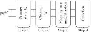
Figure 1: Block diagram of MSEQPT protocol. Step 1: Preparation of basis operator $E_{i}$ state. Step 2: Application of quantum channel $\Lambda$. Step 3: Mapping of basis operator to measurements of individual spin magnetizations followed by expectation value measurements of Pauli $z$-operators on subsystems. Step 4: Detection on individual spins.

A stepwise description of the experimental implementation of the MSEQPT protocol to selectively determine the element $\chi_{ab}$ of the process matrix is as follows:

Table 1: Fifteen observables for two qubits mapped to z-magnetization of one of the qubits. $\rho_{k}=U_{k}\Lambda(E_{i})U_{k}^{\dagger}$ in order to calculate $\langle E_{k}\rangle=\textbf{Tr}\left[E_{k}\Lambda(E_{i})\right]$.

Observable Expectation		Unitary operator $U_{k}$
$\langle\sigma_{2x}\rangle$ = Tr[$\rho_{1}.\sigma_{2z}$]		$U_{1}=\overline{Y}_{2}$
$\langle\sigma_{2y}\rangle$ = Tr[$\rho_{2}.\sigma_{2z}$]		$U_{2}=X_{2}$
$\langle\sigma_{2z}\rangle$ = Tr[$\rho_{3}.\sigma_{2z}$]		$U_{3}$=Identity
$\langle\sigma_{1x}\rangle$ = Tr$\left[\rho_{4}.\sigma_{1z}\right]$		$U_{4}=\overline{Y}_{1}$
$\langle\sigma_{1x}\sigma_{2x}\rangle$ = Tr[$\rho_{5}.\sigma_{2z}$]		$U_{5}={\rm{CNOT~{}}}Y_{2}Y_{1}$
$\langle\sigma_{1x}\sigma_{2y}\rangle$ = Tr[$\rho_{6}.\sigma_{2z}$]		$U_{6}={\rm{CNOT~{}}}\overline{X}_{2}Y_{1}$
$\langle\sigma_{1x}\sigma_{2z}\rangle$ = Tr[$\rho_{7}.\sigma_{2z}$]		$U_{7}={\rm{CNOT~{}}}\overline{Y}_{1}$
$\langle\sigma_{1y}\rangle$ = Tr[$\rho_{8}.\sigma_{1z}$]		$U_{8}=X_{1}$
$\langle\sigma_{1y}\sigma_{2x}\rangle$ = Tr[$\rho_{9}.\sigma_{2z}$]		$U_{9}={\rm{CNOT~{}}}\overline{Y}_{2}X_{1}$
$\langle\sigma_{1y}\sigma_{2y}\rangle$ = Tr[$\rho_{10}.\sigma_{2z}$]		$U_{10}={\rm{CNOT~{}}}\overline{X}_{2}\overline{X}_{1}$
$\langle\sigma_{1y}\sigma_{2z}\rangle$ = Tr[$\rho_{11}.\sigma_{2z}$]		$U_{11}={\rm{CNOT~{}}}X_{1}$
$\langle\sigma_{1z}\rangle$ = Tr[$\rho_{12}.\sigma_{1z}$]		$U_{12}$=Identity
$\langle\sigma_{1z}\sigma_{2x}\rangle$ = Tr[$\rho_{13}.\sigma_{2z}$]		$U_{13}={\rm{CNOT~{}}}\overline{Y}_{2}$
$\langle\sigma_{1z}\sigma_{2y}\rangle$ = Tr[$\rho_{14}.\sigma_{2z}$]		$U_{14}={\rm{CNOT~{}}}X_{2}$
$\langle\sigma_{1z}\sigma_{2z}\rangle$ = Tr[$\rho_{15}.\sigma_{2z}$]		$U_{15}=\rm{CNOT~{}}$

1. Choose any state $\rho_{j}=|\phi_{j}\rangle\langle\phi_{j}|$ from the set of quantum 2-design and find the decomposition of $E_{a}^{\dagger}\rho_{j}E_{b}$ in terms of basis operators $E_{i}$.

2. Experimentally prepare the quantum system in one of the basis states having non-vanishing coefficients ${}^{j}c^{ab}_{i}$ as per Equation (6).

3. Apply the quantum channel $\Lambda$ to $E_{i}$ to get the output state $\Lambda(E_{i})$.

4. Find the decomposition of the chosen state $\rho_{j}$ in terms of basis operators analytically and then experimentally determine the expectation values of all those $E_{k}$’s which have non-vanishing coefficients, ${}^{j}e_{k}$, using our measurement technique.

5. Repeat the procedure for all the states in the chosen quantum 2-design set.

The MSEQPT protocol is schematically depicted in Fig. 1: the first step is to prepare the basis state, followed by the action of the quantum process. After the quantum process has acted on the basis state the next step is to map the required measurements to single-spin magnetization measurements and finally we do the single spin magnetization detection.

Our modified scheme has two advantages: first, it is simpler than the original scheme as we do not have to choose different experimental settings for the estimation of each element of the $\chi$ matrix and second, it involves fewer experiments. The comparison of experimental resources required by different protocols to determine a specific element of the $\chi$ matrix for two-qubit systems is given in Table 2.

Table 2: Comparison of experimental resources for different protocols for the determination of a specific element of the $\chi$ matrix for a two-qubit system

	QPT	SEQPT	MSEQPT
Preparations	15	80	15
Readouts	120	240	60

The standard QPT method implemented on two NMR qubits relies on the channel action given by

$$\rho_{out}=\sum_{a,b}\chi_{ab}{E_{a}}\rho_{in}{E_{b}^{\dagger}}$$ (12)

This requires state preparation settings ($\rho_{in}$)= 15, with the number of tomographs required being 15. Since each tomograph requires 8 readouts, the total number of readouts required is $15\times 8=120$.

In the SEQPT protocol, the states to be prepared for estimating the real part of $\chi_{ab}$ are: $(E_{a}\pm E_{b})^{\dagger}\rho_{j}((E_{a}\pm E_{b}))$, where j=1 to 20 (2-design states). The states to be prepared for estimating the imaginary part of $\chi_{ab}$ are: $(E_{a}\pm iE_{b})^{\dagger}\rho_{j}((E_{a}\pm iE_{b}))$. The number of state preparation settings required to obtain $\chi_{ab}$ = 80 (20 for $(E_{a}+E_{b})$ + 20 for $(E_{a}-E_{b})$ + 20 for $(E_{a}+iE_{b})$ + 20 for $(E_{a}-iE_{b})$). This method requires 3 readouts (the number of non vanishing coefficients in the expansion of $\rho_{j}$) for each state, in order to obtain transition probabilities $\textbf{Tr}[\rho_{j}\Lambda((E_{a}\pm E_{b})^{\dagger}\rho_{j}(E_{a}\pm E_{b}))]$ and $\textbf{Tr}[\rho_{j}\Lambda((E_{a}\pm iE_{b})^{\dagger}\rho_{j}(E_{a}\pm iE_{b}))]$. Hence the total number of readouts required required for the SEQPT method is $3\times 80=240$. For the MSEQPT protocol, the number of state preparation settings are 15 while the number of readouts required for each state preparation is 4. Hence the total number of readouts required required for the MSEQPT method is $4\times 15=60$.

II.1 Quantum 2-design set using mutually unbiased basis

One of the requirements for experimental implementation of MSEQPT is the quantum 2-design set $S$, and algorithms to construct such a set are available (Dankert et al., 2009; Bendersky et al., 2009). One way is to find a complete set of mutually unbiased basis (MUBs) states where a system with a $D$ dimensional state space will have ($D+1$) MUBs if $D$ is a prime number or power of a prime number (Bandyopadhyay et al., 2002; Lawrence et al., 2002; Andreas Klappenecker, 2004). For our two-qubit system $D=2^{2}$, and the set of quantum 2-design can be constructed by using a complete set of MUBs, which are five in this case. The MUBs states satisfy the relation, ${|\langle\phi_{p}^{B_{k}}|\phi_{q}^{B_{l}}\rangle|}^{2}=\frac{1}{D}$ for all $k\neq l$, $B_{k}$’s are basis set labels and $\phi_{p}$’s are the elements within the basis set. The complete set of MUBs constituting states in quantum 2-design set for 2-qubit system $(D=4)$, in the computational basis, is given below (Andreas Klappenecker, 2004):

$$B_{1}=\left\{\begin{pmatrix}1\\ 0\\ 0\\ 0\end{pmatrix},\begin{pmatrix}0\\ 1\\ 0\\ 0\end{pmatrix},\begin{pmatrix}0\\ 0\\ 1\\ 0\end{pmatrix},\begin{pmatrix}0\\ 0\\ 0\\ 1\end{pmatrix}\right\}$$

$$B_{2}=\frac{1}{2}\left\{\begin{pmatrix}1\\ 1\\ 1\\ 1\end{pmatrix},\begin{pmatrix}1\\ 1\\ -1\\ -1\end{pmatrix},\begin{pmatrix}1\\ -1\\ -1\\ 1\end{pmatrix},\begin{pmatrix}1\\ -1\\ 1\\ -1\end{pmatrix}\right\}$$

$$B_{3}=\frac{1}{2}\left\{\begin{pmatrix}1\\ i\\ i\\ -1\end{pmatrix},\begin{pmatrix}1\\ -i\\ i\\ 1\end{pmatrix},\begin{pmatrix}1\\ i\\ -i\\ 1\end{pmatrix},\begin{pmatrix}1\\ -i\\ -i\\ -1\end{pmatrix}\right\}$$

$$B_{4}=\frac{1}{2}\left\{\begin{pmatrix}1\\ -1\\ -i\\ -i\end{pmatrix},\begin{pmatrix}1\\ -1\\ i\\ i\end{pmatrix},\begin{pmatrix}1\\ 1\\ -i\\ -i\end{pmatrix},\begin{pmatrix}1\\ 1\\ -i\\ i\end{pmatrix}\right\}$$

$$B_{5}=\frac{1}{2}\left\{\begin{pmatrix}1\\ -i\\ -1\\ -i\end{pmatrix},\begin{pmatrix}1\\ -i\\ 1\\ i\end{pmatrix},\begin{pmatrix}1\\ i\\ -1\\ i\end{pmatrix},\begin{pmatrix}1\\ i\\ 1\\ -i\end{pmatrix}\right\}$$ (13)

For example $|\phi_{3}^{B_{1}}\rangle$ is the third element of $B_{1}$ basis set and the state is $|10\rangle$. Also $B_{1}$ is the commonly used computational basis. All the twenty states in the above defined MUBs comprise the quantum 2-design set $S$ for the present study.

Figure 2: (a) Quantum circuit to implement MSEQPT. Local unitary operations $R_{\phi}^{\theta}$ are achieved via rotations by an angle $\theta$ and phase $\phi$. The values of the angles $\theta_{l}$ are either $0$ or $\frac{\pi}{2}$, depending on the experiment being performed, where $|\theta_{1}-\theta_{2}|=\frac{\pi}{2}$; a bar over a phase represents negative phase. The first and second blocks prepare the desired basis state $E_{i}$ and the second block is implemented only if $\theta_{3}=\frac{\pi}{2}$. The shaded block represents non-unitary evolution to destroy unwanted coherences. The third block represents the unitary quantum channel $\Lambda$ which takes $E_{i}\rightarrow\Lambda(E_{i})$. The last block achieves the conversion of the state $\Lambda(E_{i})$ to determine $\langle E_{i}\rangle$ by measuring either $\langle\sigma_{1z}\rangle$ or $\langle\sigma_{2z}\rangle$. (b) NMR pulse sequence for the quantum circuit given in panel (a). All unfilled rectangles denote $\pi/2$ pulses with the phase written above the pulse, while the solid rectangle denotes a $\frac{\theta}{2}$ pulse with $\bar{z}$ phase; the evolution time periods are $\tau_{0}=1/(2J_{\rm CH})$ and $\tau=\theta/(2\pi J_{\rm CH})$, respectively. The measurement box represents the time-domain NMR signal which gives the expectation value of $\sigma_{z}$ after a Fourier transform.

III NMR implementation of MSEQPT

We demonstrate the MSEQPT protocol on an NMR quantum information processor for three different unitary processes: a ‘no operation’ (NOOP), a controlled-NOT (CNOT) gate and a controlled-Hadamard (CH) gate (we have used the name CH for this gate where the Hadamard gate is in fact the standard pseudo-Hadamard gate in NMR). One of the most studied nonlocal unitary quantum processes is the entangling CNOT gate, which is a controlled bit flip of the target qubit if the control qubit is in the state $|1\rangle$, while the controlled Hadamard corresponds to applying a Hadamard (or a pseudo-Hadamard) gate to the target qubit when the controlled qubit is in the state $|1\rangle$.

Table 3: Parameters chosen to implement different unitary quantum processes.

Quantum process	Phase $\phi$	$\theta$
NOOP	$x$, $y$	0
CNOT	$x$	$\pi$
CH	$\overline{y}$	$\frac{\pi}{2}$

In Fig. 2 a general rotation through an angle $\theta$ and a phase $\phi$ on a qubit is represented by the unitary operator $R_{\phi}^{\theta}$. Table 3 lists the values for $\theta$ and $\phi$ used in the quantum circuit (Fig. 2(a)) to achieve the desired unitaries. NOOP implies ‘do nothing’ or ‘no operation’, the CNOT gate flips the state of the target qubit (and introduces a phase $e^{-\iota\frac{\pi}{2}}$) if the control qubit is in the state $|1\rangle$. The controlled-Hadamard (CH) creates a superposition state of the target qubit ($|0\rangle\rightarrow|-\rangle$ and $|1\rangle\rightarrow|+\rangle$) if the control qubit is in the state $|1\rangle$; the states $|\pm\rangle=\frac{1}{\sqrt{2}}(|0\rangle\pm|1\rangle)$; a bar over a phase represents a negative phase.

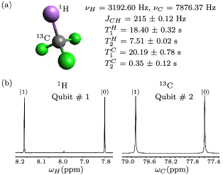
Figure 3: (Color online) (a) Molecular structure of ¹³C labeled chloroform used as a two-qubit quantum system. The first and second qubits are encoded as the nuclear spin ¹H and ¹³C, respectively. The values of the scalar coupling $J_{\rm CH}$ (in Hz) and relaxation times $T_{1}$ and $T_{2}$ (in seconds) and chemical shifts $\nu_{i}$ are shown alongside. (b) Thermal equilibrium NMR spectrum after a $\frac{\pi}{2}$ detection pulse.

As discussed in Section II we choose the Pauli operators as basis operators, $\{E_{i}\}$, although other choices of basis operators are equally valid as the quantum process being tomographed is independent of such choices. The sixteen product operators for the two-qubit system are (Ernst et al., 1990): $I$, $\sigma_{2x}$, $\sigma_{2y}$, $\sigma_{2z}$, $\sigma_{1x}$, $\sigma_{1x}\sigma_{2x}$, $\sigma_{1x}\sigma_{2y}$, $\sigma_{1x}\sigma_{2z}$, $\sigma_{1y}$, $\sigma_{1y}\sigma_{2x}$, $\sigma_{1y}\sigma_{2y}$, $\sigma_{1y}\sigma_{2z}$, $\sigma_{1z}$, $\sigma_{1z}\sigma_{2x}$, $\sigma_{1z}\sigma_{2y}$, $\sigma_{1z}\sigma_{2z}$, where $I$ is a $4\times 4$ identity matrix, the $\sigma$ are the Pauli matrices and terms such as $\sigma_{1x}\otimes\sigma_{2z}$ are written as $\sigma_{1x}\sigma_{2z}$ for simplicity. The quantum mapping for the experimental measurement of the expectation values of product operators by appropriate single-spin measurements is given in Table 1 (Singh et al., 2016b). For instance, in order to find the expectation value of $\langle\sigma_{1x}\sigma_{2y}\rangle$ in the state $\Lambda(E_{i})$, we map $\Lambda(E_{i})\rightarrow\rho_{6}$ with $\rho_{6}=U_{6}\Lambda(E_{i})U_{6}^{\dagger}$. As per Table 1, $U_{6}={\rm CNOT~{}}\overline{X}_{2}Y_{1}$ which implies that we need to have the system undergo a single-spin $\frac{\pi}{2}$ rotation of the first qubit with a phase $y$ and of the second qubit with a phase $\overline{x}$, followed by a CNOT gate. After this, $\langle\sigma_{2z}\rangle$ in the state $\rho_{6}$ is equivalent to $\langle\sigma_{1x}\sigma_{2y}\rangle$ in the state $\Lambda(E_{i})$. In the NMR scenario, it is convenient to find the expectation values for Pauli $z$-operators as they correspond to $z$ magnetizations of the nuclear spins.

We encode the two NMR qubits in a molecule of ¹³C-enriched chloroform dissolved in acetone-D6, with the nuclear spins ¹H and ¹³C labeled as ‘Qubit 1’ and ‘Qubit 2’, respectively. The molecular structure, experimental parameters and the NMR spectrum obtained at thermal equilibrium after a $\frac{\pi}{2}$ detection pulse are shown in Fig. 3. All the experiments were performed at ambient temperature on a Bruker Avance III 400 MHz FT-NMR spectrometer equipped with a BBO probe.

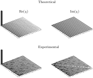
Figure 4: The tomographs in the columns denote the real and imaginary parts of the $\chi$ matrix respectively, for the NOOP case. The tomographs on the top represent the theoretically constructed while those on the bottom represent the experimentally measured $\chi$ matrix for the NOOP case. The fidelity of the NOOP turned out to be $0.98$.

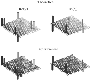
Figure 5: The tomographs in the columns denote the real and imaginary parts of the $\chi$ matrix respectively, for the CNOT gate (control-$R_{x}^{\pi}$). The tomographs on the top represent the theoretically constructed while those on the bottom represent the experimentally measured $\chi$ matrix of the CNOT operator. The fidelity of the CNOT operator turned out to be 0.93.

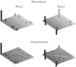
Figure 6: The tomographs in the columns denote the real and imaginary parts of the $\chi$ matrix respectively, for the controlled-Hadamard gate (control-$R_{y}^{-\frac{\pi}{2}}$). The tomographs on the top represent the theoretically constructed while those on the bottom represent the experimentally measured $\chi$ matrix of the CH operator. The fidelity of the CH operator turned out to be 0.92.

The Hamiltonian for a two-qubit system in the rotating frame is given by

$${\mathcal{H}}=2\pi\left[(\nu_{{\rm H}}-\nu_{{\rm H}}^{{\rm rf}})I_{z}^{{\rm H}}+(\nu_{{\rm C}}-\nu_{{\rm C}}^{{\rm rf}})I_{z}^{{\rm C}}+J_{{\rm CH}}I_{z}^{{\rm H}}I_{z}^{{\rm C}}\right]$$ (14)

where $\nu_{{\rm H}}$, $\nu_{{\rm C}}$ are the chemical shifts and $I_{z}^{{\rm H}}$, $I_{z}^{{\rm C}}$ are the z-components of the spin angular momentum operators of the ¹H and ¹³C spins respectively, and J_CH is the scalar coupling constant; $\nu_{{\rm H}}^{{\rm rf}}$ and $\nu_{{\rm C}}^{{\rm rf}}$ are the rotating frame frequencies. We used the spatial averaging technique to prepare the spins in an initial pseudopure state (Cory et al., 1998; Oliveira et al., 2007):

$$\rho_{00}=\frac{1}{4}(1-\epsilon)I+\epsilon|00\rangle\langle 00|$$ (15)

where $\epsilon$ is proportional to spin polarization and can be evaluated from the ratio of magnetic and thermal energies of an ensemble of magnetic moments $\mu$ in a magnetic field $B$ at temperature $T$; $\epsilon\thicksim\frac{\mu B}{k_{B}T}$ and at room temperature and for a $B\approx$ 10 Tesla, $\epsilon\approx\rm{10^{-5}}$.

The quantum circuit and the corresponding NMR pulse sequence for implementation of the MSEQPT scheme are shown in Figs. 2(a) and 2(b), respectively. The circuit is divided into four modules, separated by dashed blue lines. The unitary $R_{\phi}^{\theta}$ in the circuit represents a local rotation through an angle $\theta$ and phase $\phi$. All the rotation angles are either zero or $\frac{\pi}{2}$. The first two modules of the circuit prepare the required basis state $E_{i}$. The shaded rectangle in the first part of the quantum circuit represents a non-unitary quantum process to destroy unwanted quantum coherences. The second module is implemented only if the experimental settings require a nonzero $\theta_{3}$. The third model corresponds to the unitary quantum process $\Lambda$ which takes $E_{i}\rightarrow\Lambda(E_{i})$. The last modules executes the quantum mapping, as per Table 1, of the desired operator $E_{i}$ to single-spin Pauli $z$-operators. The meter symbol represents an NMR measurement and only one of the three measurements takes place in one experimental setting. The quantum gates (and local rotations) were implemented using highly accurate radio frequency (rf) pulses and free evolution periods under the system Hamiltonian. Spin selective hard pulses of desired phase were used for local rotations; for $\rm{{}^{1}H}$ a $\frac{\pi}{2}$ hard pulse corresponds to an rf pulse of duration 12.95 $\mu$s at 20.19 W power level while for $\rm{{}^{13}C}$ the pulse duration was 8.55 $\mu$s at 74.67 W power level. All the unfilled rectangles denote $\frac{\pi}{2}$ hard pulses while the filled rectangle is a $\frac{\theta}{2}$ hard pulse as dictated by the unitary quantum process $\Lambda$. The phases of all hard pulses are written above the respective pulse. A $z$-gradient was used to kill the undesired coherences during basis state preparation. The measurement boxes denote the time-domain NMR signal which is proportional to the expectation value of $\sigma_{z}$ after a Fourier transformation.

The fidelity of experimentally constructed $\chi_{\rm{expt}}$ with reference to theoretically expected $\chi_{\rm{theo}}$ was calculated using the measure (Zhang et al., 2014):

$${\mathcal{F}}(\chi_{\rm expt},\chi_{\rm theo})=\frac{|{\rm Tr}[\chi_{\rm expt}\chi_{\rm theo}^{\dagger}]|}{\sqrt{{\rm Tr}[\chi_{\rm expt}^{\dagger}\chi_{\rm expt}]{\rm Tr}[\chi_{\rm theo}^{\dagger}\chi_{\rm theo}]}}$$ (16)

Fidelity measure ${\mathcal{F}}$ is normalized in the sense that as $\chi_{\rm{expt}}\rightarrow\chi_{\rm{theo}}$ i.e. experimentally constructed $\chi$ matrix approaches theoretically expected $\chi$ matrix leads to ${\mathcal{F}}$ $\rightarrow$ 1.

The theoretically constructed and experimentally tomographed $\chi$ matrices for the NOOP, the CNOT and the CH gates are depicted in Fig. 4–6, respectively. The fidelity ${\mathcal{F}}$ for NOOP, CNOT and CH operators was found to be 0.98, 0.93 and 0.92 respectively. The upper panel in Fig. 4 depicts the theoretically expected $\chi$ matrix while the lower panel depicts the experimentally constructed $\chi$ matrix (real and imaginary parts) for the NOOP case. Axes of the $\chi$ matrix are labeled by the indices of the product basis operators $E_{i}$. Similarly Figs. 5 and 6 are the $\chi$ matrices for CNOT and CH operators respectively. In all three cases the fidelity F was greater than 0.92 which signifies the successful experimental implementation of the MSEQPT protocol.

IV Concluding Remarks

In this study, we proposed a scheme for selective and efficient quantum process tomography appropriate for NMR systems. Our scheme has a marked advantage in terms of using fewer experiments to determine the selected elements of the process matrix. We successfully demonstrated the experimental implementation of the scheme for ‘no operation’, a controlled-NOT and a controlled-Hadamard gate on two NMR qubits. The method is both selective and efficient and can hence be very useful in any quantum process which does not require a full experimental characterization of the process matrix. Furthermore, the important task of calculating the closeness between the implemented process and the targeted process can be efficiently estimated in a selective manner. While our modified protocol offers a clear advantage for the NMR quantum process tomography experiments, its utility in other experimental techniques needs to be explored further. Efforts are on to implement the modified protocol for more general quantum processes and for a larger number of qubits.