X-ray Eclipses of Active Galactic Nuclei

Abstract

X-ray variation is a ubiquitous feature of active galactic nuclei (AGNs), however, its origin is not well understood. In this paper, we show that the X-ray flux variations in some AGNs, and correspondingly the power spectral densities (PSDs) of the variations, may be interpreted as being caused by absorptions of eclipsing clouds or clumps in the broad line region (BLR) and the dusty torus. By performing Monte-Carlo simulations for a number of plausible cloud models, we systematically investigate the statistics of the X-ray variations resulting from the cloud eclipsing and the PSDs of the variations. For these models, we show that the number of eclipsing events can be significant and the absorption column densities due to those eclipsing clouds can be in the range from $10^{21}$ to $10^{24}{\text{cm}}^{-2}$, leading to significant X-ray variations. We find that the PSDs obtained from the mock observations for the X-ray flux and the absorption column density resulting from these models can be described by a broken double power law, similar to those directly measured from observations of some AGNs. The shape of the PSDs depend strongly on the kinematic structures and the intrinsic properties of the clouds in AGNs. We demonstrate that the X-ray eclipsing model can naturally lead to a strong correlation between the break frequencies (and correspondingly the break timescales) of the PSDs and the masses of the massive black holes (MBHs) in the model AGNs, which can be well consistent with the one obtained from observations. Future studies of the PSDs of the AGN X-ray (and possibly also the optical-UV) flux and column density variations may provide a powerful tool to constrain the structure of the BLR and the torus and to estimate the MBH masses in AGNs.

1 Introduction

X-ray variation is a ubiquitous feature of active galactic nuclei (AGNs; e.g., Mushotzky et al. 1993). The variation timescale of the AGN X-ray emission ranges from hours, days, to years (e.g., McHardy & Czerny, 1987; Mushotzky et al., 1993; Markowitz et al., 2003). Observations have revealed that the power spectral density (PSD) of the X-ray variation as a function of the variation frequency $\nu$ in many AGNs, $P(\nu)$, can be described by a double power law with a break frequency of $\nu_{\rm B}$, i.e., $P(\nu)\propto\nu^{\gamma_{h}}$ at high frequencies ($\nu\gg\nu_{\rm B}$) with $\gamma_{h}\lesssim-2$, and $P(\nu)\propto\nu^{\gamma_{l}}$ at low frequencies ($\nu\ll\nu_{\rm B}$) with $\gamma_{l}\sim-1$ (e.g. McHardy & Czerny, 1987; Uttley et al., 2002; Markowitz et al., 2003; González-Martín & Vaughan, 2012). It has been demonstrated that the characteristic timescales corresponding to the break frequencies ($\sim 1/\nu_{\rm B}$) strongly correlate with the masses of the central massive black holes (MBHs) in those AGNs (McHardy et al., 2006; González-Martín & Vaughan, 2012). The properties of some X-ray binaries (XRBs) could also fit into this correlation (e.g., McHardy et al., 2006), but the reliability of such a relationship is not clear, yet (e.g., Done & Gierliński, 2005; Körding et al., 2007). The physics behind the break frequency versus BH mass correlation is not well understood so far.

A number of models have been proposed to explain the observed X-ray variation of AGNs. In general, these models can be divided into the two main categories: (1) the variation is due to changes in the intrinsic X-ray emission; and (2) the variation is due to changes in the materials or clouds along the line of sight (LOS) to the X-ray emitting source that absorb part of the intrinsic X-ray emission. In the first category, the X-ray variation could be due to the change of the accretion rate, and consequently, to the change of the total number of seed photons to be inverse Compton-scattered up to X-ray photons by the hot corona located in the vicinity of the central MBHs of AGNs (e.g., Lyubarskii, 1997; Lamer et al., 2003a; Uttley et al., 2002; Zdziarski et al., 2003), or to the change of the hot corona itself (including its motion and location), or to the inflation of the magnetic flares being injected into the corona (e.g., Poutanen & Fabian, 1999; Lu & Yu, 2001a; Fabian & Vaughan, 2003; Marinucci et al., 2014). In the second category, the X-ray variation is dominated by the absorption of clouds in multiple zones that (partially) cover the X-ray emitting source on the observer’s sky plane (e.g., Lamer et al., 2003b; Turner & Miller, 2009; Miller et al., 2008, 2009; Parker et al., 2015; Abrassart & Czerny, 2000). In the standard AGN unification model (Antonucci, 1993), the natural sources for the absorption are some line emission clouds in the broad line region (BLR) or some clumps in the dusty torus that happen to cross the LOS; hereafter, we refer to all of them as absorption clouds for simplicity, unless otherwise stated. This kind of absorption model appears to be able to explain well not only the X-ray variations of some AGNs, such as MCG-6-30-15, NGC 4395, NGC 4151, and NGC 1365 (Turner & Miller, 2009; Parker et al., 2015), but also the relative lack of variability at the higher energy band of the X-ray emission (e.g., Miller et al., 2008). The X-ray variation patterns and consequently the PSDs of the variations resulted from these two model categories should be distinguishable from each other since their physical origins are quite different. The study of the origin of X-ray variations would provide an insight into the structure of and the radiation mechanisms in the central engine of AGNs.

In the scenario where the observed X-ray variations for some AGNs are mainly caused by absorption, when a cloud crosses the LOS, a fraction of the X-ray photons are absorbed depending on the physical properties of the cloud, and the rest penetrate through the cloud and are received by the distant observer. For such an event, we denote it as an “X-ray eclipse” in this paper. The duration of an X-ray eclipse event and the period of the events are affected by the velocity of the cloud and its distance to the central engine. For example, the clouds located at large distances may lead to long-term variations because of their relatively low velocities, while those located at small distances may lead to short-term variations. If many clouds spreading over a large range of distances can lead to X-ray eclipses, the X-ray variation timescales or frequencies will depend on both the geometric and the kinematic distributions of those clouds and the physical properties of individual clouds. The PSD of the X-ray variation curves describes the distribution of power into the variation frequency components composing the X-ray variations, and the analysis of the PSD provides a powerful tool to statistically study the kinematical and physical conditions of those eclipsing clouds located at different spatial regions and further their parent populations (clouds in the BLR and clumps in the dusty torus of AGNs).

In this paper, we construct an X-ray cloud eclipsing model, and this model generates many observational properties of X-ray variations in AGNs, including the PSD and the break frequency versus BH mass correlation mentioned above. We use Monte-Carlo simulations to consider the kinematical motion of the clouds and clumps in the BLR and the dusty torus, and realize the X-ray eclipsing events over a long period and consequently generate mock observations of the X-ray flux variation. We also investigate the dependence of the PSDs obtained from the mock observations on the kinematic structure and the intrinsic properties of the clouds. Note here that we only consider those AGNs in which the X-ray variations are dominated by the absorption of eclipsing clouds. For simplicity, we do not intend to simultaneously consider the X-ray variations caused by the changes in the intrinsic X-ray emission, which may dominate the detected variations in some other AGNs.

The paper is organized as follows. In Section 2, we construct the X-ray eclipsing model and analyze the event rate and the properties of the X-ray eclipses by assuming that the eclipsing clouds are from the BLR and the dusty torus. We investigate the dependence of the rate and the properties of the X-ray eclipses on the kinematic and spatial structure of the parent population of the eclipsing clouds and the intrinsic properties of those clouds. By adopting a number of different models for the spatial distribution and the properties of the clouds, we perform some Monte-Carlo simulations to realize X-ray eclipses and generate mock X-ray light curves in Section 3. According to those mock X-ray light curves, we obtain their PSDs in Section 4 and we find that they are compatible with the reasonable parameter ranges for the spatial and kinematical distributions and the physical properties of the eclipsing clouds. We also demonstrate that a strong correlation between the break frequency of the PSD and the MBH mass is a natural result of the scenario where the X-ray variation is dominated by the absorption of eclipsing clouds, if the inner boundary for the spatial distribution of the absorption clouds and some intrinsic properties of those clouds scale (linearly) with the MBH mass. Discussions and conclusions are given in Section 5.

In this paper, given a set of physical variables $\mathbf{X}=(X_{1},...,X_{k})$ (e.g., semimajor axis, eccentricity), the probability distribution function (PDF) of $\mathbf{X}$ is denoted by $f_{\mathbf{X}}(\mathbf{X})$ so that $f_{\mathbf{X}}(\mathbf{X})d\mathbf{X}$ represents the number fraction of clouds with the variable $X_{i}$ being in the range $X_{i}\rightarrow X_{i}+dX_{i}$ ($i=1,..,k$) with $\int f_{\mathbf{X}}(\mathbf{X})d\mathbf{X}=1$, where $d\mathbf{X}\equiv dX_{1}...dX_{k}$.

2 Model for the eclipsing of X-ray emission

X-ray emission from AGNs received by a distant observer may vary due to absorptions by clouds crossing the LOS, as revealed by observations of some type 1 and type 2 Seyfert galaxies. The variation timescales of the X-ray emission and the possible locations of the absorption clouds cover a wide range as follows. (1) Some of those absorption events have durations of about a few hours to a few days and absorption column hydrogen densities $\sim 10^{22}-10^{24}{\rm cm}^{-2}$, which are probably due to some clouds in the BLR with number densities of $10^{9}-10^{11}{\rm cm}^{-3}$ and distance $\sim 10^{3}-10^{4}r_{\rm g}$ from the central MBH, where $r_{\rm g}\equiv GM_{\bullet}/c^{2}$ is the gravitational radius of the MBH with mass $M_{\bullet}$ (e.g., Lamer et al. 2003b; Maiolino et al. 2010; Sanfrutos et al. 2013; Bianchi et al. 2009; Markowitz et al. 2014; Risaliti et al. 2005, 2007, 2009; Puccetti et al. 2007). (2) Some other events have durations up to several months, substantially longer than those due to the BLR clouds, and absorption column hydrogen densities $\sim 10^{22}-10^{23}{\rm cm}^{-2}$, which may be attributed to the clumps located in the outer dusty torus with number densities of $\sim 10^{7}-10^{8}{\rm cm}^{-3}$ (e.g. Rivers et al., 2011; Marinucci et al., 2013; Miniutti et al., 2014; Agís-González et al., 2014; Markowitz et al., 2014). Based on those observations, we introduce simple models below to systematically study the eclipsing of X-ray emission from AGNs.

2.1 Spatial Distribution of Clouds

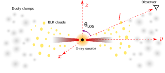
Figure 1: An illustration diagram for the spatial distribution of clouds (as a population) surrounding the central engine of an AGN. The black dot at the center represents the central MBH, and the two thick shaded bars along the y-axis represent a thin accretion disk surrounding the MBH. The orange region at the center represents the X-ray emitting region, probably the corona structure above the accretion disk. The absorption clouds include both the BLR clouds outside of the accretion disk (yellow) and the dusty clumps (gray) in the dusty torus outside of the broad line region (BLR). The spatial distribution of the clouds is assumed to be axisymmetric. The direction of the line of sight (LOS), i.e., the viewing angle, is defined by the angle of $\theta_{{\rm LOS}}$ with respect to the symmetric axis of the system ($z$), and the LOS is on the $yz$ plane.

Figure 1 shows a schematic picture for the spatial distribution of numerous clouds rotating around the central engine, an MBH-accretion disk system with enormous X-ray emission. These clouds are located in the two different regions, i.e., the BLR and the dusty torus. The motions of those clouds are probably dominated by the gravity of the central MBH (for the BLR clouds, see Gaskell 1988; Koratkar & Gaskell 1991; Sergeev et al. 1999; for the clumps in the dusty torus, see Elitzur & Shlosman 2006; Nenkova et al. 2008), and other effects, such as the radiation pressure, on the cloud motion may be negligible. For simplicity, we assume that all of those clouds and clumps are spherical and are in Keplerian motion and on circular orbits around the central MBH..

To describe the motion of each cloud and the spatial distribution of those clouds as a population, we use both an orthogonal coordinate system ($x,y,z$) and a spherical coordinate system ($r,\theta,\phi$), with the origin located at the central MBH. Here, $r$ is the distance to the central MBH, $\theta$ is the polar angle defined relative to the $z$-axis perpendicular to the accretion disk, and $\phi$ is the azimuth angle (see Fig. 1). The spherical coordinate system is linked to the orthogonal one by $(x,y,z)=(r\sin\theta\cos\phi,r\sin\theta\sin\phi,r\cos\theta)$. We set the distant observer to be on the $yz$ plane with a direction of $(\theta,\phi)=(\theta_{\rm LOS},\pi/2)$, and the unit vector of this direction is $\hat{\mathbf{\ell}}=(0,\sin\theta_{\rm LOS},\cos\theta_{\rm LOS})$ in the ($x,y,z$) coordinate system.

For a single cloud in a Keplerian motion, its orbit is determined by a set of parameters $\mathbf{X}=(a_{\rm c},\theta_{J},\phi_{J})$, where $a_{\rm c}$ are the semimajor axis of the orbit, and $\theta_{J}$ and $\phi_{J}$ are the two angles defining the normal $\hat{n}_{J}$ of the orbital plane with $\hat{n}_{J}$=$(\sin\theta_{J}\cos\phi_{J},\sin\theta_{J}\sin\phi_{J},\cos\theta_{J})$. Given the initial position of a cloud, its position at any given moment can be obtained with that set of parameters. Each of those circular orbits can then be described by the set of parameters, and the spatial distribution of those clouds as a population can be described by a PDF $f_{\mathbf{X}}(\mathbf{X})$. Assuming that the system is axisymmetric and the distribution of $a_{\rm c}$ is independent of the distribution of the normal of the orbital plane, the PDF can be further reduced to $f_{a_{\rm c}}(a_{\rm c})|f_{\cos\theta_{J}}(\cos\theta_{J})\sin\theta_{J}|/(2\pi)$.

2.2 Eclipsing Events due to Individual Clouds

If a cloud crosses the LOS and is in front of the central engine, then an eclipse occurs and the cloud partially or completely blocks the X-ray emitting region. In the image plane of the observer, the trajectory of any eclipsing event can be described by the two parameters, i.e., the impact parameter ($b$) and the eclipsing angle ($\Omega$), as shown in Figure 2. The eclipsing angle $\Omega$ is defined as the angle between the motion direction of the cloud in the image plane and a reference direction (the horizontal line from left to right in Fig. 2, i.e., the direction anti-parallel to the $x$-axis in Fig. 1), and it is given by

$$\cos\Omega = -\hat{v}_{yz}\cdot\hat{e}_{x}=-[\hat{n}_{J}\times(\hat{n}_{J}\times\hat{e}_{x})]\cdot\hat{e}_{x}$$ (1)

$$= \frac{\cos\theta_{J}}{|\cos\theta_{J}|}\sqrt{1-\sin^{2}\theta_{J}\cos^{2}\phi_{J}},$$

and

$$\sin\Omega=\sin\theta_{J}\cos\phi_{J},$$ (2)

where $\hat{v}_{yz}$ is a unit vector with the same direction as the velocity of a cloud when it crosses the $yz$ plane, and $\hat{e}_{x}=(1,0,0)$ is a unit vector at the direction of the $x$-axis. If $\phi_{J}=\pi/2$ and $\theta_{J}\in[0,\pi/2)$, then $\Omega=0$; if $\phi_{J}=\pi/2$ and $\theta_{J}\in(\pi/2,\pi]$, then $\Omega=\pi$. If $\theta_{J}=\pi/2$, then $\Omega$ is either $\pi/2-\phi_{J}$ or $\phi_{J}-\pi/2$.

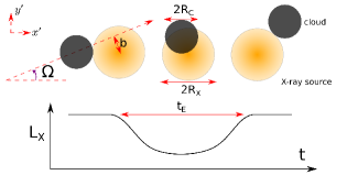
Figure 2: Schematic diagram for an X-ray eclipsing event by a cloud crossing the LOS. The absorption cloud may be a cloud in the BLR region or a dusty clump, as shown in Figure 1. The top row of this figure illustrates three phases of the eclipse, i.e., the ingress phase (left), the greatest eclipse phase (middle), and the egress phase (right). The observer is located at the direction of pointing outward of the surface, with the $(x^{\prime},y^{\prime})$ coordinate system on the surface. The X-ray emitting region is assumed to be spherical with a radius size of $R_{\rm X}$. The transiting direction on the sky plane of the observer is determined by the impact parameter $b$ and the direction angle $\Omega$ relative to a reference direction (e.g., the horizontal line). The intervening cloud that leads to the eclipse is also assumed to be spherical with a radius size of $R_{\rm c}$. The duration of the eclipsing event is $t_{\rm E}$. The bottom plot illustrates the variation of the X-ray flux due to the eclipse.

The impact parameter $b$ is defined by

$$b \equiv a_{\rm c}(\hat{n}_{J}\cdot\hat{\mathbf{\ell}})=a_{\rm c}\cos\omega$$ (3)

$$= a_{\rm c}(\sin\theta_{J}\sin\phi_{J}\sin\theta_{\rm LOS}+\cos\theta_{J}\cos\theta_{\rm LOS})$$

for $|b|\ll a_{\rm c}$ or $\cos\omega\ll 1$, which is true for all of the cases considered in this paper since the size of the central X-ray source is much smaller than the semimajor axes of the absorption clouds. The $\omega$ in Equation (3) is the angle between the normal of the orbital plane of a cloud and the LOS. We have $b=0$ when $\phi_{J}=\pi/2$ and $\theta_{J}=\pi/2+\theta_{\rm LOS}$ (or more generally, when $\sin\phi_{J}=-\cot\theta_{J}\cot\theta_{\rm LOS}$). A cloud crosses the LOS clockwise (or counter-clockwise) with respect to the center of the X-ray source if $b<0$ (or $b>0$).

Assuming that the X-ray emitting region is spherical with a radius size of $R_{\rm X}$ and a spherical cloud with a radius size of $R_{\rm c}$ crosses the LOS, an eclipsing event occurs when $|b|<R_{\rm c}+R_{\rm X}$. The following phases during this eclipsing event are illustrated in Figure 2: (1) an ingress phase when the cloud starts to block the X-ray emission; (2) a maximum eclipsing phase when the cloud blocks the projected X-ray emission region as much as it can or even completely block the region, which leads to a dip in the X-ray light curve; and (3) an egress phase when the part of the cloud that first moved into the projected X-ray emission region starts to move out.

The duration of an eclipsing event caused by a cloud is

$$t_{\rm E}\simeq 2\left[(R_{\rm X}+R_{\rm c})^{2}-b^{2}\right]^{1/2}(a_{\rm c}/GM_{\bullet})^{1/2},$$ (4)

where the cloud size $R_{\rm c}$ is assumed to be a function of $a_{\rm c}$. If the eclipse event starts at a time $t_{\rm s}$, the center of the cloud in the image plane is given by

$$x^{\prime}_{\rm c} = -b\sin\Omega+D_{\rm E}\left(\frac{t-t_{\rm s}}{{t_{\rm E}}}-\frac{1}{2}\right)\cos\Omega,$$ (5)

$$y^{\prime}_{\rm c} = b\cos\Omega+D_{\rm E}\left(\frac{t-t_{\rm s}}{{t_{\rm E}}}-\frac{1}{2}\right)\sin\Omega,$$ (6)

where $D_{\rm E}=2\sqrt{(R_{\rm X}+R_{\rm c})^{2}-b^{2}}$, $t_{\rm s}<t<t_{\rm s}+t_{\rm E}$, and $t_{\rm s}$ is the start time of the eclipse.

At any given time, the observational flux or luminosity curve is obtained by

$$L_{\rm X}\equiv\iint I(x^{\prime},y^{\prime})A_{\nu}(N_{\rm H}(R_{\rm c},r_{x\rm c}))dx^{\prime}dy^{\prime},$$ (7)

where $I(x^{\prime},y^{\prime})$ is the intrinsic surface brightness of the X-ray emission at a position $(x^{\prime},y^{\prime})$ on the image plane and $I(x^{\prime},y^{\prime})=0$ if $x^{\prime 2}+y^{\prime 2}>R^{2}_{\rm X}$, $N_{\rm H}(R_{\rm c},r_{\rm Xc})$ is the projected column density at a distance $r_{\rm Xc}=\sqrt{[x^{\prime}_{\rm c}(t)-x^{\prime}]^{2}+[y^{\prime}_{\rm c}(t)-y^{\prime}]^{2}}$ from the cloud center on the image plane, and $A_{\nu}$ represents the fraction of X-ray photons penetrating through the cloud and received by the distant observer, with $A_{\nu}=1$ for the unblocked region with $x^{\prime 2}+y^{\prime 2}\leq R^{2}_{\rm X}$ and $A_{\nu}<1$ for the blocked region. (Note here that the X-ray eclipsing discussed in this paper is different from the cases of planet transits, for which the emission from the area of a star covered by a front planet is completely blocked, i.e., $A_{\nu}=0$.) The ratio of the observational X-ray flux to the intrinsic one (without eclipsing) is

$$R_{L_{\rm X}}\equiv\frac{L_{\rm X}}{L_{\rm X,0}}=\frac{\iint I(x^{\prime},y^{\prime})A_{\nu}(N_{\rm H}(R_{\rm c},r_{\rm Xc}))dx^{\prime}dy^{\prime}}{\iint I(x^{\prime},y^{\prime})dx^{\prime}dy^{\prime}}.$$ (8)

If the hydrogen number density ($n_{\rm H}$) of a cloud is uniform, i.e., $n_{\rm H}$ is a constant within the cloud, then $N_{\rm H}(R_{\rm c},r_{\rm Xc})=2n_{\rm H}\sqrt{R^{2}_{\rm c}-r^{2}_{\rm Xc}}$ for $r_{\rm Xc}\leq R_{\rm c}$ and $0$ for $r_{\rm Xc}>R_{\rm c}$. If the X-ray emissivity is also uniform, then $I(x^{\prime},y^{\prime})\propto\sqrt{R^{2}_{\rm X}-x^{\prime 2}-y^{\prime 2}}$. If the X-ray surface brightness is homogeneous, then $I(x^{\prime},y^{\prime})$ is a constant, we have

$$R_{L_{\rm X}}=\frac{\iint A_{\nu}(N_{\rm H}(R_{\rm c},r_{\rm Xc}))dx^{\prime}dy^{\prime}}{\pi R^{2}_{\rm X}}.$$ (9)

We define an “effective column density” as

$$N_{\rm H,eff}\equiv A_{\nu}^{-1}(R_{L_{\rm X}}),$$ (10)

where $A_{\nu}^{-1}$ is the inverse function of $A_{\nu}$. The effective column density may correspond to the absorption column density directly measured from observations.

The bottom panel of Figure 2 illustrates the X-ray variation due to an eclipsing event. The detailed calculations of the X-ray variations at a given frequency range due to eclipsing events are described in Section 3.

For individual AGNs, we expect that a number of X-ray eclipsing events can be detected over a substantially long observational period. It is also possible that more than one cloud crosses the LOS at the same time and covers (part of) the X-ray source, which lead to complex X-ray variations (see Figure 6). For such a case, $N_{\rm H,eff}$ at a given time is roughly the summation of the effective column density due to each of the LOS crossing clouds. The statistics of those X-ray eclipsing events should depend on the spatial distribution of the absorbing clouds in the AGN and the intrinsic properties of those clouds.

2.3 Event Rates of the X-ray Eclipses

Given the total number of the clouds $N_{\rm tot}$ and their spatial probability distribution function, the event rate of the X-ray eclipses caused by the clouds with parameters $\mathbf{X}$ within the range $\mathbf{X}\rightarrow\mathbf{X}+d\mathbf{X}$ can be given by

$$d\mathscr{R}=\frac{N_{\rm tot}f_{\mathbf{X}}(\mathbf{X})}{T_{\rm orb}(a_{\rm c})}d\mathbf{X},$$

$$= da_{\rm c}d\cos\theta_{J}d\phi_{J}\frac{N_{\rm tot}f_{a_{\rm c}}(a_{\rm c})}{2\pi T_{\rm orb}(a_{\rm c})}f_{\cos\theta_{J}}(\cos\theta_{J}),$$

$$= -da_{\rm c}dbd\Omega\frac{N_{\rm tot}f_{a_{\rm c}}(a_{\rm c})}{2\pi T_{\rm orb}(a_{\rm c})}f_{\cos\theta_{J}}(\cos\theta_{J})\sin\theta_{J}\left|\frac{\partial(\theta_{J},\phi_{J})}{\partial(b,\Omega)}\right|,$$

where $T_{\rm orb}(a_{\rm c})=2\pi(a_{\rm c}^{3}/GM_{\bullet})^{1/2}$ is the orbital period of a cloud with semimajor axis $a_{\rm c}$, $\frac{\partial(\theta_{J},\phi_{J})}{\partial(b,\Omega)}$ is the Jacobian determinant, $\Omega$ and $b$ are given by Equations (1)–(3), $\Omega\in(0,2\pi]$, $b\in[-R_{X}-R_{\rm c}(a_{\rm c}),R_{X}+R_{\rm c}(a_{\rm c})]$, $a_{\rm c}\in[a_{\rm c,min},a_{\rm c,max}]$, and $a_{\rm c,min}$ and $a_{\rm c,max}$ are the smallest and the largest values for the semimajor axes of those clouds, respectively.

For most of the eclipsing clouds, we have $\cos\omega\simeq 0$ and $\omega\simeq\pi/2$ since $b\ll a_{\rm c}$, and $\left|\frac{\partial(\theta_{J},\phi_{J})}{\partial(b,\Omega)}\right|=\frac{\sin\omega}{a_{\rm c}\sin\theta_{J}}\simeq\frac{1}{a_{\rm c}\sin\theta_{J}}$. Therefore, we approximately have $\cos\theta_{J}\simeq\sin\theta_{{\rm LOS}}\cos\Omega$ according to Equations (2) and (3), and the integration of Equation (LABEL:eq:eventrate) can be further reduced to

$$\mathscr{R} = \int d\mathscr{R}$$ (12)

$$\simeq {N_{\rm tot}R_{\rm X}}\int^{\infty}_{0}\frac{f_{a_{\rm c}}(a_{\rm c})\left[1+R_{\rm c}(a_{\rm c})/R_{\rm X}\right]}{a_{\rm c}T_{\rm orb}(a_{\rm c})}da_{\rm c}$$

$$\times\int^{2\pi}_{0}\frac{f_{\cos\theta_{J}}(\sin\theta_{\rm LOS}\cos\Omega)}{\pi}d\Omega,$$

$$= N_{\rm tot}\mathscr{H}(\theta_{\rm LOS})\frac{(GM_{\bullet})^{1/2}R_{\rm X}}{2\pi\left<a_{\rm E}\right>^{5/2}}$$

$$\simeq 1.4{\rm day}^{-1}\mathscr{H}(\theta_{\rm LOS})\left(\frac{10^{7}M_{\odot}}{M_{\bullet}}\right)\left(\frac{N_{\rm tot}}{10^{7}}\right)\times$$

$$\left(\frac{R_{\rm X}}{5r_{\rm g}}\right)\left(\frac{\left<a_{\rm E}\right>}{10^{4}r_{\rm g}}\right)^{-5/2},$$

where $\mathscr{H}(\theta_{\rm LOS})\equiv\int^{2\pi}_{0}d\Omega f_{\cos\theta_{J}}(\sin\theta_{{\rm LOS}}\cos\Omega)/\pi$ is determined by the distribution of the angular momenta of the clouds and the direction of the LOS. If $f_{\cos\theta_{J}}$ is a uniform distribution, i.e., $f_{\cos\theta_{J}}=1/2$, then $\mathscr{H}(\theta_{\rm LOS})=1$. The effective semimajor axis of the eclipsing clouds $\left<a_{\rm E}\right>$ is defined by

$$\left<a_{\rm E}\right>^{-5/2}=\int^{\infty}_{0}da_{\rm c}f_{a_{\rm c}}(a_{\rm c})\left[1+R_{\rm c}(a_{\rm c})/R_{\rm X}\right]/a^{5/2}_{\rm c},$$ (13)

which is mainly determined by $f_{a_{\rm c}}(a_{\rm c})$. It may also depend on the ratio of the size of the eclipsing clouds to the size of the X-ray emitting region if the cloud size depends on the semimajor axis of the cloud.

According to Equation (12), the distribution function of the semimajor axis of those eclipsing clouds is given by

$$f_{a_{\rm c},\rm E}(a_{\rm c})=\frac{\langle a_{\rm E}\rangle^{5/2}}{a_{\rm c}^{5/2}}f_{a_{\rm c}}(a_{\rm c})\left[1+\frac{R_{\rm c}(a_{\rm c})}{R_{\rm X}}\right].$$ (14)

This PDF indicates that the X-ray eclipsing events are preferentially contributed by those clouds at relatively close distances to the central MBH or those clouds with relatively large sizes (see also the bottom-right panel in Figure 5 below).

2.4 Mean number of the clouds crossing the line of sight at a given time

The mean number of the clouds crossing the LOS at a given time is

$$\langle N\rangle_{\rm LOS} = \int t_{\rm E}d\mathscr{R},$$

$$\simeq -\int^{\infty}_{0}da_{\rm c}\int^{R_{X}+R_{\rm c}}_{-R_{X}-R_{\rm c}}db$$

$$\times\int^{2\pi}_{0}d\Omega\frac{N_{\rm tot}f_{a_{\rm c}}(a_{\rm c})t_{\rm E}}{2\pi a_{\rm c}T_{\rm orb}(a_{\rm c})}f_{\cos\theta_{J}}(\sin\theta_{\rm LOS}\cos\Omega)$$

$$\simeq 0.6\mathscr{H}(\theta_{\rm LOS})\left(\frac{N_{\rm tot}}{10^{7}}\right)\left(\frac{R_{X}}{5r_{\rm g}}\right)^{2}\left(\frac{\langle a_{N}\rangle}{10^{4}r_{\rm g}}\right)^{-2},$$

where $t_{\rm E}$ in Equation (4) is used and $\langle a_{\rm N}\rangle$ is defined through

$$\langle a_{\rm N}\rangle^{-2}=\int\left[1+R_{\rm c}(a_{\rm c})/R_{X}\right]^{2}\left[f_{a_{\rm c}}(a_{\rm c})/a_{\rm c}^{2}\right]da_{\rm c}.$$ (16)

Note here that the dependence of $\langle N\rangle_{\rm LOS}$ on the MBH mass is only through the dependence of $N_{\rm tot}$ or $\mathscr{H}(\theta_{\rm LOS})$ on the MBH mass, if the size of the X-ray source and $\left<a_{\rm N}\right>$ scale linearly with the gravitational radius of the central MBH (and the MBH mass). According to Equation (LABEL:eq:nlos), $\langle N\rangle_{\rm LOS}\propto\langle a_{N}\rangle^{-2}$, the number of clouds crossing the LOS depends on the size and spatial distribution of the clouds. Similar to $\mathscr{R}$, $\langle N\rangle_{\rm LOS}$ also scales linearly with the total number of clouds and depends on $\mathscr{H}(\theta_{\rm LOS})$ (see also the top-right panel of Figure 5 below).

2.5 Statistical Properties of the Eclipsing Events

The trajectory of an eclipsing event on the sky plane is described by the impact parameter $b$ and the eclipsing angle $\Omega$, and the time duration of an eclipse is determined by $t_{\rm E}$. The statistical distribution of those parameters may be helpful for understanding the X-ray variability resulting from the X-ray eclipsing events.

2.5.1 Probability distribution of the impact parameter

The PDF of the impact parameter $|b|$ for an eclipse detected at any given time is given by

$$f_{|b|}(|b|) = \frac{1}{\mathscr{R}}\frac{\partial}{\partial|b|}\int d\mathscr{R}$$ (17)

$$= -\frac{N_{\rm tot}}{\mathscr{R}}\frac{\partial}{\partial|b|}\int^{\infty}_{0}da_{\rm c}\frac{f_{a_{\rm c}}(a_{\rm c})}{a_{\rm c}T_{\rm orb}(a_{\rm c})}$$

$$\times\int^{R_{X}+R_{\rm c}(a_{\rm c})}_{|b|}d|b|^{\prime}\int^{2\pi}_{0}\frac{f_{\cos\theta_{J}}(\sin\theta_{\rm LOS}\cos\Omega)}{\pi}d\Omega$$

$$= \frac{1}{R_{X}}\frac{\int^{\infty}_{a_{\rm c,l}}f_{a_{\rm c}}(a_{\rm c})a_{\rm c}^{-5/2}da_{\rm c}}{\langle a_{\rm E}\rangle^{-5/2}},$$

where $a_{\rm c,l}={\rm max}[R^{-1}_{\rm c}(|b|-R_{X}),a_{\rm c,min}]$ if $|b|>R_{X}$, $a_{\rm c,l}=a_{\rm c,min}$ if $|b|\leq R_{X}$, and $R^{-1}_{\rm c}(|b|-R_{X})$ is an inverse function of $R_{\rm c}(a_{\rm c})=|b|-R_{X}$. If all of the clouds have the same size, then $f_{|b|}(|b|)=\frac{1}{R_{X}+R_{\rm c}}$ for $|b|\leq R_{X}+R_{\rm c}$. For more general cases, such as those models listed in Table 1, $f_{|b|}(|b|)$ is a constant when $|b|\leq R_{X}+R_{\rm c,min}$, and decreases with increasing $|b|$ when $|b|>R_{X}+R_{\rm c,min}$, where $R_{\rm c,min}$ is the minimum radius size of the clouds (see more on size distribution in Section 3.3).

2.5.2 Probability distribution of the eclipse angle

For any given LOS, the PDF of $\Omega$ is given by

$$f_{\Omega}(\Omega)\simeq\frac{f_{\cos\theta_{J}}(\sin\theta_{\rm LOS}\cos\Omega)}{\pi\mathscr{H}(\theta_{\rm LOS})}.$$ (18)

As seen from equation (18), the PDF $f_{\Omega}$ is mainly determined by the spatial distribution of those eclipsing clouds (or their parent population).

We note here that, in principle, the profile of the Fe K$\alpha$ line emission, if any, from the inner disk of an AGN depends on the disk structure. If the eclipsing events frequently occur with different $(b,\Omega)$, the changes of the Fe K$\alpha$ profile during those events are determined by both the parameters $(b,\Omega)$ (Risaliti et al., 2011) and the inner disk structure (or the emissivity law of the line). Therefore, the variation of the Fe K$\alpha$ line emission due to eclipsing may also be used to probe the kinematic structure of the parent population of the eclipsing clouds and the inner disk structure.

2.5.3 Probability Distribution of the Eclipse Timescale

The PDF of the eclipse timescale $t_{\rm E}$ can be obtained by

$$f_{t_{\rm E}}(t_{\rm E})=\frac{1}{\mathscr{R}}\frac{\partial}{\partial t_{\rm E}}\int d\mathscr{R},$$

$$= \frac{N_{\rm tot}}{E}\frac{\partial}{\partial t_{\rm E}}\int^{\infty}_{0}da_{\rm c}\frac{f_{a_{\rm c}}(a_{\rm c})}{a_{\rm c}T_{\rm orb}(a_{\rm c})}$$

$$\times\int^{R_{X}+R_{\rm c}(a_{\rm c})}_{\sqrt{[R_{X}+R_{\rm c}(a_{\rm c})]^{2}-\frac{GM_{\bullet}t_{\rm E}^{2}}{4a_{\rm c}}}}db^{\prime}\int^{2\pi}_{0}\frac{f_{J}(\sin\theta_{\rm LOS}\cos\Omega)}{\pi}d\Omega,$$

$$= \int^{\infty}_{0}\frac{\langle a_{\rm E}\rangle^{5/2}}{a_{\rm c}^{5/2}}\left[1+\frac{R_{\rm c}(a_{\rm c})}{R_{\rm X}}\right]\frac{t_{\rm E}}{t^{\prime}_{\rm E}(a_{\rm c})}\frac{f_{a_{\rm c}}(a_{\rm c})da_{\rm c}}{\sqrt{t^{\prime}_{\rm E}(a_{\rm c})^{2}-t_{\rm E}^{2}}},$$

where

$$t^{\prime}_{\rm E}(a_{\rm c})=2[R_{\rm X}+R_{\rm c}(a_{\rm c})]/\sqrt{GM_{\bullet}/a_{\rm c}}$$ (20)

is the maximum eclipse duration (when $b=0$). The mean duration of the eclipsing events is given by $\langle t_{\rm E}\rangle=\int t_{\rm E}f_{t_{\rm E}}(t_{\rm E})dt_{\rm E}=\langle N\rangle_{\rm LOS}/\mathscr{R}$, which can be further reduced to

$$\langle t_{\rm E}\rangle = 0.45~{}{\rm day}\left(\frac{M_{\bullet}}{10^{7}M_{\odot}}\right)\left(\frac{R_{X}}{5r_{g}}\right)\left(\frac{\langle a_{E}\rangle}{10^{4}r_{g}}\right)^{5/2}\left(\frac{\langle a_{N}\rangle}{10^{4}r_{g}}\right)^{-2}.$$

According to Equation (LABEL:eq:te_avg), $\langle t_{\rm E}\rangle\propto M_{\bullet}$ if $R_{X}$, $\langle a_{\rm E}\rangle$ and $\langle a_{N}\rangle$ all scale linearly with the mass of the central MBH. The typical eclipsing duration for AGNs with central MBH mass in the range from $10^{6}M_{\odot}$ to $10^{9}M_{\odot}$ is $\langle t_{\rm E}\rangle\sim 0.05$ to $\sim 50$ days, which can be monitored by most currently available X-ray missions. Note that the eclipsing time $t_{\rm E}$ due to individual clouds can be as long as $10^{3}$ days for those clouds located at the outer part of the torus, or as short as $10^{-1}$ days for clouds located at the inner part of the BLR (see the bottom-left panel of Figure 5).

3 Monte-Carlo Simulations of the X-ray Eclipses

In this section, we use Monte-Carlo simulations to realize the kinematical motion of the clouds in AGNs and the X-ray eclipses. We adopt eight models for the spatial distribution and the intrinsic properties of the clouds as listed in Table 1. Some settings for the parameters involved in the cloud model are well motivated by observations as described below. The details of the Monte-Carlo simulations are described in Section 3.5 and the simulation results are presented in Section 3.6.

3.1 Settings on the Spatial Distribution of the Clouds

Observations have shown that different broad emission lines are originated from gas clouds or clumps at different distances from the central illuminating source. Those line-emitting clouds and clumps are distributed over a large spatial extent, from the inner edge of the BLR to the outer region of the dusty torus. The high ionization emission lines (CIV, HeII, etc.) are originated from a region closer to the central MBH than the low ionization emission lines (H$\beta$, HeI, etc.) (e.g., Gaskell & Sparke, 1986; Kaspi et al., 2000; Peterson et al., 2004; Landt et al., 2008; Bentz et al., 2010; Pancoast et al., 2011). Some lines in the infrared (IR), e.g., OI, Pa$\epsilon$, Br$\gamma$, are emitted from a region even farther away, extending to the dust sublimation radius $r_{\rm d}$, the presumed inner edge of the dusty torus (Landt et al., 2008; Markowitz et al., 2014). It was also suggested that the torus may be a smooth continuation of the BLR (Schartmann et al., 2005; Suganuma et al., 2006; Elitzur & Shlosman, 2006). We thus assume that the radial distribution of those clouds and clumps can be described by a simple power-law function, and we will not analyze them separately in this paper.

Infrared reverberation mapping observations have shown that the dust sublimation radius is roughly given by

$$r_{\rm d} \simeq 0.40{\rm pc}\left(\frac{L_{\rm bol}}{10^{45}{\rm erg\,s}^{-1}}\right)^{1/2}\left(\frac{T_{\rm sub}}{1500\,{\rm K}}\right)^{2.6}$$ (22)

$$\simeq 0.45{\rm pc}\lambda^{1/2}_{\rm Edd}\left(\frac{M_{\bullet}}{10^{7}M_{\odot}}\right)^{1/2}\left(\frac{T_{\rm sub}}{1500{\rm\,K}}\right)^{2.6},$$

where $L_{\rm bol}$ is the AGN bolometric luminosity, $\lambda_{\rm Edd}\equiv L_{\rm bol}/L_{\rm Edd}$ is the Eddington ratio, $L_{\rm Edd}\simeq 1.3\times 10^{45}{\rm erg\,s}^{-1}(M_{\bullet}/10^{7}M_{\odot})$ is the Eddington luminosity, and $T_{\rm sub}$ is the dust sublimation temperature (Suganuma et al., 2006; Nenkova et al., 2008). For all of the models listed in Table 1, we assume that $T_{\rm sub}=1500$ K and $\lambda_{\rm Edd}=0.1$, since observations suggest that most AGNs (and QSOs) accrete material via a rate close to $0.1-0.3$ (e.g., Kollmeier et al., 2006; Shen et al., 2008). If $M_{\bullet}=10^{7}M_{\odot}$, $r_{\rm d}$ is approximately $3\times 10^{5}r_{\rm g}$.

We assume that the radial distribution of those clouds (and clumps) follows a broken power law with a transition radius $r_{\rm t}$, i.e.,

$$f_{a_{\rm c}}(a_{\rm c})\propto\begin{cases}\left(a_{\rm c}/r_{\rm t}\right)^{\alpha_{a_{\rm c},1}},&\quad\text{for }a_{\rm c}\leq r_{\rm t},\\ \left(a_{\rm c}/r_{\rm t}\right)^{\alpha_{a_{\rm c},2}},&\quad\text{for }a_{\rm c}>r_{\rm t}.\end{cases}$$ (23)

The slopes $\alpha_{a_{\rm c},1}$ and $\alpha_{a_{\rm c},2}$ control the radial distribution of those clouds. For example, for a lower $\alpha_{a_{\rm c},1}$, relatively more clouds are located in the inner region; and for a larger $\alpha_{a_{\rm c},2}$, relatively more clouds are located in the outer region. The transition radius $r_{\rm t}$ may be proportional to the dust sublimation radius $r_{\rm d}$, roughly the boundary between the BLR and the dusty torus. The reason is that the gas clumps (or clouds) in the region outside of the sublimation radius may be significantly less affected by the radiation from the central source than those clouds within that radius. For all of the models in Table 1, we assume that $r_{\rm t}\sim 0.1r_{\rm d}$. In models C1-C4, the clouds are more concentrated in the inner region compared with those in models A1, A2, B1, and B2; the clouds are more concentrated in the outer region in models B1 and B2 compared with those in the other models. How the model results depend on the parameter settings, i.e., the inner and the outer boundaries for the spatial distribution of clouds, the Eddington ratio, and the transition radius $r_{\rm t}$ is discussed in Section 4.

The PDF of the orbital planes (or the direction of the orbital angular momenta) of those clouds over the solid angle is denoted as $f_{\cos\theta_{J}}(\cos\theta_{J})/2\pi$, i.e., the fraction per solid angle ($|d\cos\theta_{J}d\phi_{J}|$). If the PDF of $f_{\cos\theta_{J}}(\cos\theta_{J})$ is uniform, then $f_{\cos\theta_{J}}(\cos\theta_{J})=1/2$. However, the spatial distribution of the clouds is probably flattened (e.g, Bentz et al., 2010; Li et al., 2013). Considering this flattening, we assume that the distribution of $\theta_{J}$ follows a Schwarzschild or Rayleigh distribution with

$$f_{\cos\theta_{J}}(\cos\theta_{J})d\cos\theta_{J}\propto\theta_{J}e^{-\frac{\theta_{J}^{2}}{2\sigma^{2}_{\theta_{J}}}}d\theta_{J},$$ (24)

where we set $\sigma_{\theta_{J}}=\pi/9$ for all of the models listed in Table 1. Considering that the distribution in Equation (24) was derived with a small $\theta_{J}$ approximation, we also try the following distribution

$$f_{\cos\theta_{J}}(\cos\theta_{J})d\cos\theta_{J}\propto\sin\theta_{J}e^{-\frac{\sin^{2}\theta_{J}}{2\sigma^{2}_{\sin\theta_{J}}}}d\theta_{J},$$ (25)

where $\sigma_{\sin\theta_{J}}=\sin(\pi/9)$. The total angular momentum of the clouds is none-zero in the distribution of Equation (24), and zero in Equation (25), which represents some extreme case of the kinematic distribution of the clouds. We find that choosing a different $\sigma_{\theta_{J}}$ or a different distribution function of $f_{\cos\theta_{J}}(\cos\theta_{J})$ affects only the function $\mathscr{H}(\theta_{\rm LOS})$, and thus $\mathscr{R}$ and $\langle N\rangle_{\rm LOS}$ (which can be obtained straightforwardly from Equations 12 and LABEL:eq:nlos), but not the shape of the PSDs. For simplicity, we only present the results obtained by using Equation (24).

Table 1: Parameters in the cloud models

A1	1	-0.5	$10^{3}$	2	1	1	-1.5	$-4.0\pm 0.3$	$-0.94\pm 0.08$	$2.1\pm 0.6$	$-3.9\pm 0.2$	$-1.0\pm 0.1$	$2.2\pm 0.6$
A2	1	-0.5	$10^{3}$	2	1	1	-1	$-4.0\pm 0.1$	$-1.5\pm 0.1$	$2.5\pm 0.7$	$-3.7\pm 0.2$	$-1.4\pm 0.1$	$2.5\pm 0.9$
B1	1	0	$10^{3}$	2	1	1	-1.5	$-4.2\pm 0.2$	$-1.0\pm 0.1$	$2.3\pm 0.7$	$-4.0\pm 0.4$	$-1.1\pm 0.1$	$2.7\pm 0.9$
B2	1	0	$10^{2}$	0.2	1	60	-1.5	$-4.2\pm 0.2$	$-1.12\pm 0.03$	$1.6\pm 0.3$	$-4.0\pm 0.2$	$-1.17\pm 0.04$	$1.8\pm 0.4$
C1	0	-0.5	$10^{3}$	2	1	1	-1.5	$-6.3\pm 0.2$	$-0.88\pm 0.02$	$0.41\pm 0.09$	$-6.4\pm 0.2$	$-0.98\pm 0.03$	$0.4\pm 0.3$
C2	0	-0.5	$10^{2}$	0.2	1	60	-1.5	$-2.8\pm 0.1$	$-0.81\pm 0.08$	$1.8\pm 0.3$	$-2.6\pm 0.2$	$-0.91\pm 0.03$	$1.6\pm 0.3$
C3	0	-0.5	$10^{2}$	0.2	1	$10^{2}$	-2	$-2.3\pm 0.1$	$-0.20\pm 0.04$	$1.6\pm 0.4$	$-2.11\pm 0.09$	$-0.18\pm 0.04$	$1.7\pm 0.5$
C4	0	-0.5	$10^{2}$	0.6	0.5	60	-1.5	$-2.56\pm 0.09$	$0.39\pm 0.03$	$0.4\pm 0.1$	$-2.7\pm 0.2$	$0.33\pm 0.04$	$0.27\pm 0.08$

3.2 $N_{\rm tot}$

The total number of the clouds in the BLR and the dusty torus can be estimated for some sources according to the fluctuations in the emission line profiles caused by a finite number of discrete line emitters. For example, Dietrich et al. (1999) estimated that the total number of the clouds in the BLR of 3C 273 is $\sim 10^{8}$; Arav et al. (1997) and Laor et al. (2006) put a lower limit of $3\times 10^{6}$ and $\sim 10^{4}-10^{5}$ on the number of BLR clouds for Mrk 335 and NGC 4395, respectively; Arav et al. (1998) found that the total number of the clouds in the BLR of NGC 4151 has to be $\sim 3\times 10^{7}-10^{8}$ in order to generate the observed profile of the emission lines. However, it is not clear whether the total number of the clouds in the BLR and the dusty torus depends on AGN properties, e.g., the MBH mass, the Eddington ratio. For simplicity, we assume that the total number of clouds is $N_{\rm tot}=10^{7}$ for those AGN models investigated in this paper. We have also further checked that choosing a different $N_{\rm tot}$, say, $10^{6}$ or $10^{8}$, does affect our estimates on the eclipsing event rate ($\mathscr{R}$) and the mean number of clouds crossing the LOS at any given time ($\langle N\rangle_{\rm LOS}$), but does not affect our results on the shape of the PSD presented in Section 4.

3.3 Settings on the Intrinsic Properties of the Clouds

The detected X-ray eclipsing events in some AGNs so far suggest that the sizes of the eclipsing clouds should be on the order of $\sim 1-10^{2}r_{\rm g}$ (e.g., Sanfrutos et al., 2013; Markowitz et al., 2014). It also appears that the sizes of the eclipsing clouds increase with their increasing distances from the central engine (Markowitz et al., 2014). However, the exact distribution of the sizes of the eclipsing clouds and their parent population is not currently known. For simplicity, we assume that the radius size of a cloud depends on its semimajor axis, i.e.,

$$R_{\rm c}(a_{\rm c})=R_{\rm c,0}(a_{\rm c}/a_{\rm c,min})^{\alpha_{R_{\rm c}}},$$ (26)

where $R_{\rm c,0}$ is the size of those clouds located at the inner edge of the BLR ($a_{\rm c,min}$). As listed in Table 1, we set $(\alpha_{R_{\rm c}},R_{\rm c,0})=(1,2r_{\rm g})$ for the models A1, A2, B1, and C1; $(\alpha_{R_{\rm c}},R_{\rm c,0})=(1,0.2r_{\rm g})$ for the models B2, C2, and C3; and $(\alpha_{R_{\rm c}},R_{\rm c,0})=(0.5,0.6r_{\rm g})$ for the model C4. With these settings, the clouds at a distance of $\simeq 10^{3}r_{\rm g}$ from the central engine have almost the same size ($\simeq 2r_{\rm g}$) in all of these models; the filling factor of the clouds within the outer boundary $\lesssim 1.4$ pc (for $M_{\bullet}=10^{7}M_{\odot}$) is much smaller than one; and the covering factor is in the range of $0.5-0.8$, compatible with the constraints obtained from infrared observations of the torus (e.g., Ichikawa et al., 2015; Nenkova et al., 2008).

Note here that the possible collisions among the clouds are ignored in this study. In reality, those clouds in the BLR and the dusty torus may be on eccentric orbits and their velocities disperse, so that they may collide with each other and be destroyed. The collision rate can be roughly estimated by $\sim N_{\text{{\rm tot}}}\Sigma\Delta v/V$, where $\Sigma\sim\pi\langle R^{2}_{\text{c}}\rangle$ is the mean cross section of those clouds, $\langle R^{2}_{\text{c}}\rangle$ is the mean of the square radius of those clouds, $\Delta v$ is the mean velocity dispersion, and $V$ is the volume. If $\Delta v$ is on the order of the Keplerian velocity, we find that the collision rate is roughly a few times of $10^{-5}$ per year or less per cloud, for $N_{\text{tot}}=10^{7}$ and the size distribution of the clouds listed in Table 1, which verifies the validity of ignoring collisions in a period of less than a hundred years investigated in this study.

We assume that the hydrogen density in a single cloud is uniform and it depends on the distance of the cloud from the central engine. Observations suggest that the densities of BLR clouds correlate with the FWHM of the broad emission lines and the typical hydrogen densities of BLR clouds are in the range of $10^{8}-10^{11}{\rm cm}^{-3}$ or even bigger (e.g., Peterson 1997; Osterbrock & Ferland 2006). Therefore, we assume that the hydrogen densities of the clouds follow a power-law function of their distance to the central MBH, i.e.,

$$n_{\rm H}=n_{\rm H,0}(a_{\rm c}/a_{\rm c,min})^{\alpha_{n_{\rm H}}},$$ (27)

where $n_{\rm H,0}$ is the hydrogen density of those clouds that are the closest to the central MBH with $a_{\rm c}=a_{\rm c,min}$. The value of the power-law index is in the range of $-2<\alpha_{n_{\rm H}}<0$. For the models listed in Table 1, we set $\alpha_{n_{\rm H}}=-1$ for model A2, $\alpha=-2$ for model C3, and $\alpha=-1.5$ for all of the other models. We set the density $n_{\rm H,0}=6\times 10^{11}{\rm cm}^{-3}$ at $a_{\rm c,min}=10^{2}r_{\rm g}$ for models B2, C2, and C4, and $n_{\rm H,0}=10^{11}{\rm cm}^{-3}$ at $a_{\rm c,min}=10^{3}r_{\rm g}$ for all of the other models. According to these settings, we have $n_{\rm H}\simeq 10^{11}{\rm cm}^{-3}$ at $a_{\rm c}=10^{3}r_{\rm g}$ for all of the models in Table 1.

3.4 Size of the X-ray Emitting Region

Observations have suggested that the X-ray emitting region of AGNs is close to the central MBH and its size is small. For example, Dai et al. (2010) find that the sizes of the X-ray emitting regions in some lensed QSOs are smaller than $10r_{\rm g}$ by using the microlensing technique to map the structure of the accretion disks around those QSOs; Markowitz et al. (2014) find a similar size for the X-ray emitting region by using individual X-ray eclipsing events (see also Lamer et al., 2003b; Sanfrutos et al., 2013). For simplicity, we set $R_{X}=5r_{\rm g}$ for all the models in this paper. In principle, the sizes of the emitting regions in different AGNs can be somewhat different from each other. The effects of the different choices of $R_{\rm X}$ on our results are discussed in Section 4.

For simplicity, we also assume that the brightness distribution of the X-ray source is homogeneous. If alternatively we assume that the emissivity is uniform, we find no significant difference in the model results presented in this paper.

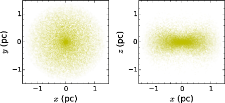
Figure 3: Illustration map for the spatial distribution of those clouds resulting from model C1 (see Table 1). The left and right panels show the face-on view and the edge-on view, respectively.

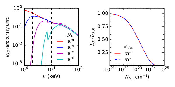
Figure 4: Left panel: the mock observational X-ray spectra resulting from different absorption column densities. The red, blue, magenta, and cyan lines represent the results for an absorption of $N_{\rm H}=10^{21}$, $10^{22}$, $10^{23}$, and $10^{24}$ cm^-2, respectively. The dashed and the solid lines with the same color represent the results for the case with a view angle of $\theta_{\rm LOS}=60{{}^{\circ}}$ and $30{{}^{\circ}}$, respectively. Here the view angle is relevant because it needs to be set in the model $\rm pexrav$ for generating the K$\alpha$ emission line and the reflection component. Right panel: the ratio of the mock observed flux ($L_{X}$) to the intrinsic X-ray flux ($L_{X,0}$) at the $2-10$ keV band as a function of the absorption column density obtained from the model phabs*pexrav in the Xspec package. The red solid and the blue dashed lines show the results for the cases with $\theta_{\rm LOS}=30{{}^{\circ}}$ and $60{{}^{\circ}}$, respectively. See Section 3.5 for the details of the model parameters.

3.5 Variations of the Absorption Column Density and the X-ray Emission

With the above settings, we perform Monte-Carlo simulations to follow the Keplerian motions of the parent population of those eclipsing clouds with random initial orbital true anomalies. At any given moment, the positions of all of the clouds on the sky plane of the observer (with a view angle of $\theta_{\rm LOS}$) can be obtained. As an example, Figure 3 shows the spatial distribution of the clouds generated from model C1, in which the clouds are centrally concentrated because of $\alpha_{n_{\rm H}}<0$. All of the clouds that happen to transit the X-ray emitting region and lead to X-ray eclipses can be identified at any given moment for each model. The changes of the absorption column densities and the X-ray flux with time can then be obtained according to the description in Section 2.2 and the procedures below. In the meantime, we can also obtain the total number of clouds across the LOS ($\langle N\rangle_{\rm LOS}$; see Eq. (LABEL:eq:nlos)) and the event rate of eclipses ($\mathscr{R}$); see Eq. (12)).

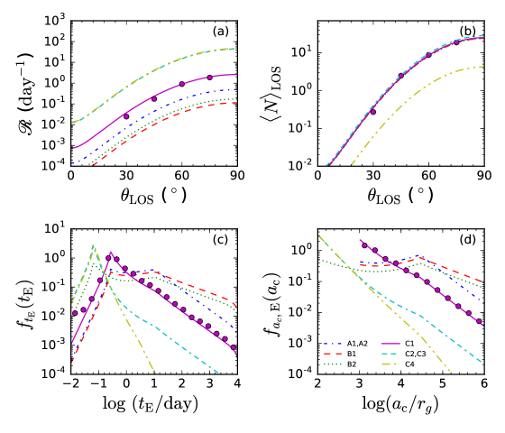
Figure 5: Statistical properties of the X-ray eclipses resulting from those models listed in Table 1. Panels (a) and (b) show the event rate of the X-ray eclipses ($\mathscr{R}$) and the time-averaged number of the eclipses ($\langle N\rangle_{\rm LOS}$) as a function of the viewing angle $\theta_{\rm LOS}$, respectively. Panels (c) and (d) show the PDFs for the time of eclipse ($f_{t_{\rm E}}(t_{\rm E})$) and the semimajor axes of the eclipsing clouds ($f_{a_{\rm c},\rm E}(a_{\rm c})$; Eq. 14), respectively. The different colors in the panels represent the results from the different models, as indicated by the text in panel (d). In each panel, the lines represent the results obtained from the analytical estimations presented in Section 2, and the magenta circles represent the results obtained from the Monte-Carlo simulations described in Section 3. For view clarity, we only show the Monte-Carlo simulation results for one model (C1), as the Monte-Carlo simulation results are well consistent with the analytical estimations. Since $f_{t_{\rm E}}(t_{\rm E})$ and $f_{a_{\rm c},\rm E}(a_{\rm c})$ are independent of the view angle $\theta_{\rm LOS}$ for all the models, here we only show the results for those models obtained by assuming $\theta_{\rm LOS}=60{{}^{\circ}}$ in panels (c) and (d).

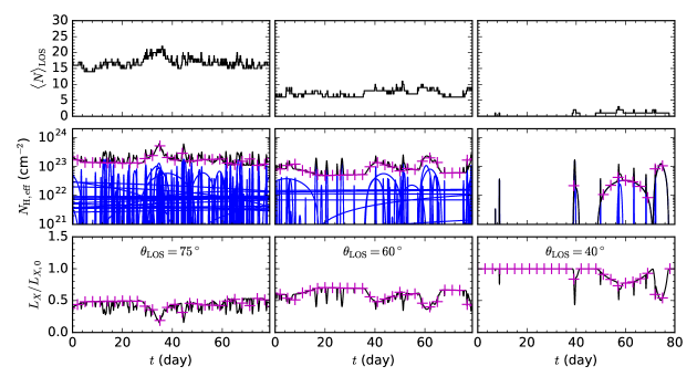
Figure 6: Evolution curves for the number of the eclipsing clouds ($\langle N\rangle_{\rm LOS}$; top panels), the absorption column density due to the eclipses ($N_{\rm H,eff}$; Eq. 10; middle panels), and the mock observations of the $2-10$ keV flux ($L_{X}$) relative to the intrinsic $2-10$ keV X-ray flux ($L_{X,0}$; bottom panels) obtained for model C1. The black and the blue lines in the middle panels represent the total column density and the contribution by the individual clouds across the LOS, respectively. The viewing angle $\theta_{\rm LOS}$ is set to $75{{}^{\circ}}$, $60{{}^{\circ}}$, and $40{{}^{\circ}}$ in the left, middle, and right panels, respectively. The magenta crosses in the middle and bottom panels mimic the observational samples collected in every $3$ days. As seen from the figure, the absorption at a given time is caused by multiple clouds if $\theta_{\rm LOS}$ is high and mainly caused by a single cloud if $\theta_{\rm LOS}$ is low.

The modeled X-ray light curves of an AGN is generated by a combination of the transmitted flux of a power-law intrinsic X-ray emission through the absorption cloud(s) and that of its reflection component. The software XSPEC, version 12.8.1, is adopted to generate the mock spectra for those modeled AGNs by $\rm phabs*pexrav$, where the pexrav is the disk reflection model (Magdziarz & Zdziarski, 1995) with a canonical power-law index of $-1.8$, and the input column density is given by $N_{\rm H,eff}(t)$ obtained from our simulations. The X-ray flux variations $L_{\rm X}(t)$ at the $2-10$ keV band can then be obtained by integrating the mock X-ray spectra. We find that a slight deviation to the canonical power-law index leads to little change in the model results. We also find negligible difference when changing the working model to $\rm phabs*powerlaw$, i.e., an absorbed pure power-law model, as the reflection component is $\lesssim 5\%$ of the total flux in the $2-10$ keV band. For simplicity, the reflection component from individual clouds is ignored.

In this paper, we focus on the $2-10$ keV band because the cloud absorption of the X-ray emission in this band is sensitive to the column density when $10^{21}\lesssim N_{\rm H,eff}\lesssim 10^{24}{\rm cm}^{-2}$, similar to the range of the effective absorption column density currently detected for the eclipsing AGNs (e.g., Risaliti et al., 2002). To demonstrate this, the left panel of Figure 4 shows the mock observational spectra resulted from the several cases with column densities of $10^{21}$, $10^{22}$, $10^{23}$, and $10^{24}{\rm cm}^{-2}$, respectively; the right panel of Figure 4 shows the ratio of the mock flux to the intrinsic X-ray flux in the $2-10$ keV band. As seen from Figure 4, if $N_{\rm H,eff}\lesssim 2\times 10^{20}{\rm cm}^{-2}$, the absorption is insignificant; and if $N_{\rm H,eff}\gtrsim 4\times 10^{24}{\rm cm}^{-2}$, the source is Compton-thick and almost all X-ray radiation at $2-10$ keV are absorbed. The absorption column densities resulting from all of the models discussed in this paper are indeed in the range from $\sim 10^{21}$ to $10^{24}~{}{\rm cm}^{-2}$ in most of the cases.

We obtain the variation curves for the mock X-ray flux $L_{\rm X}(t)$ and the mock column density $N_{\rm H,eff}(t)$ with time intervals of $\delta t$ within a period of $T_{\rm tot}$. Note that the PSDs derived from the variations of the mock X-ray flux and absorption column density (see Section 4) are valid within the frequency range $T_{\rm tot}^{-1}\lesssim\nu\lesssim\delta t^{-1}$. We set $\delta t=10^{-3}$ days and $T_{\rm tot}=10^{5}$ days, which covers the frequency range of the estimated PSDs for some AGNs, with $\nu\sim 10^{-3}$–$10^{-9}$ Hz, (e.g. McHardy & Czerny, 1987; Uttley et al., 2002; Markowitz et al., 2003; González-Martín & Vaughan, 2012). Note that the adopted $T_{\rm tot}$ is longer than the currently available observation period on the long-term X-ray variations of AGNs. Choosing a sufficiently long $T_{\rm tot}$ is reasonable for the purpose of this paper so that the shape of the PSDs revealed from our Monte-Carlo simulations in Section 4 below spans a sufficiently wide frequency range. With the adopted values of $\delta t$ and $T_{\rm tot}$, we have $\delta t\ll T_{\rm B}\ll T_{{\rm tot}}$ ($T_{\rm B}=1/\nu_{\rm B}$ in Eq. 29), and the adopted time resolution is sufficiently high and the total time duration is sufficiently long for the convergence of the model results.

3.6 Results

Figure 5 shows the statistical properties of the X-ray eclipses obtained for those models listed in Table 1. The curves in the figure represent the results obtained from the analytical estimates presented in Section 2. As the Monte-Carlo simulation results are quite consistent with the corresponding analytical estimates, we only show the Monte-Carlo simulation results of one model (C1) in Figure 5 for view clarity. As seen from Figure 5(a), the event rate $\mathscr{R}$ depends strongly on the viewing angle $\theta_{\rm LOS}$ simply because of the dependence on the function $\mathscr{H}(\theta_{\rm LOS})$ (see Eq. 12). For those models with the same viewing angle, $\mathscr{R}$ also strongly depends on the average semimajor axis of the cloud ensemble $\langle a_{\rm E}\rangle$ (Eq. 13), which is determined by the radial and the size distributions of the eclipsing clouds. Choosing a different distribution of the sizes of the eclipsing clouds and/or a different inner boundary for the clouds ($a_{\rm c,min}$) leads to a different event rate. Those models with more clouds located at the inner region (models C1-C4) generally have larger event rates compared with those models with more clouds located at the outer region (models B1 and B2). For models A1 and A2, the majority of the clouds are located at intermediate distances to the central MBH so that the event rates of the eclipses are also intermediate compared with the other models.

Figure 5(b) shows the mean number of the eclipsing clouds ($\langle N\rangle_{\rm LOS}$) for different models, which are compatible with the observational constraints for some AGNs (e.g., Nenkova et al., 2008; Ichikawa et al., 2015). As shown in this panel, $\langle N\rangle_{\rm LOS}$ depends on the viewing angle because of the assumed flattening of the spatial distribution for the parent population of the eclipsing clouds. According to Equation (LABEL:eq:nlos), $\langle N\rangle_{\rm LOS}$ also depends on $\langle a_{N}\rangle$, which is determined by $f_{a_{\rm c}}(a_{\rm c})$, $R_{\rm c}(a_{\rm c})$, and $R_{X}$. Note that the $\langle N\rangle_{\rm LOS}$ resulting from models A1, A2, B1, B2, and C1-C3 are similar for a fixed viewing angle, as shown in panel (b). In all of these models, $\alpha_{a_{\rm c}}=1$ and $\langle a_{\rm N}\rangle^{-2}\propto\int[1+R_{\rm c}(a_{\rm c})/R_{\rm X}]^{2}f_{a_{\rm c}}(a_{\rm c})a^{-2}_{\rm c}da_{\rm c}\sim$constant, which coincidentally leads to quite similar $\langle N\rangle_{\rm LOS}$ because $\langle N\rangle_{\rm LOS}\propto\langle a_{N}\rangle^{-2}$. In model C4, $\alpha_{k_{\rm c}}=0.5$, i.e., the sizes of the majority of the clouds are set to be substantially smaller than those in other models, and thus $\langle N\rangle_{\rm LOS}$ is much smaller than that from other models.

Figure 5(c) and (d) show the distribution of the time periods of eclipses [$f_{t_{\rm E}}(t_{\rm E})$; Eq. LABEL:eq:pdte] and the distribution of the semimajor axes of eclipsing clouds [$f_{a_{\rm c},\rm E}(a_{\rm c})$; Eq. 14], respectively. For models B1 and B2, relatively more clouds are located at large distances, and thus there are relatively more eclipses with long periods, compared with those of the other models. For models B2, C2, C3, and C4, the inner boundary for the clouds is smaller, and thus there are relatively more eclipses with short periods ($\lesssim 1$ day), compared with those of the other models (A1, A2, B1, and C1). The sharp decrease of $f_{t_{\rm E}}(t_{\rm E})$ at the short-timescale end is mainly due to the cutoff of the semimajor axes at $a_{\rm c,min}$ for the eclipsing clouds. As seen from Figure 5, $f_{t_{\rm E}}(t_{\rm E})$ and $f_{a_{\rm c},\rm E}(a_{\rm c})$ also strongly depend on the size distribution of the clouds ($R_{c}(a_{c})$). For model C4, the sizes of clouds are set to be substantially smaller than those clouds in other models, especially at large $a_{\rm c}$, which leads to a sharp decrease of the number of eclipses with large $a_{\rm c}$.

Figure 6 shows the evolution curves for the number of eclipsing clouds ($\langle N\rangle_{\rm LOS}$; top panels), the absorption column density ($N_{\rm H,eff}$; Eq. 10; middle panels), and the ratio of the “observed” X-ray flux to the intrinsic X-ray flux ($L_{X}/L_{X,0}$; bottom panels) obtained from the simulations for model C1, respectively. The absorption column density contributed by each individual eclipse cloud (the blue solid lines) are also shown in the middle panels. Among them, the long-time variations of both the X-ray flux and the column density are due to the eclipsing clouds in the dusty torus; the short-time variations are due to the eclipsing clouds in the BLR. As seen from Figure 6, the absorption structures are complex if the viewing angle is large (e.g., $\theta_{\rm LOS}=75^{\circ}$) because the absorption at any given time can be due to multiple clouds (the left middle and bottom panels), while it is relatively simple if the viewing angle is small (e.g., $\theta_{\rm LOS}=40^{\circ}$) because the absorption is caused by individual eclipsing clouds occasionally (the right middle and bottom panels). According to Figure 6, the presumption adopted in many previous studies that the observed variations of the absorption column density is due to single eclipsing clouds may not be realistic (e.g., Risaliti et al., 2009; Nardini & Risaliti, 2011; Sanfrutos et al., 2013; Markowitz et al., 2014).

3.7 Reconstruction and Decomposition of Individual Eclipses

In principle, the individual eclipsing events can be reconstructed by using the evolution curves of the X-ray flux and the absorption column density. The information on the properties of those eclipsing clouds may thus provide strong constraints on the spatial distribution and the intrinsic properties of their parent population as demonstrated in some previous studies (e.g., Sanfrutos et al., 2013). However, it is usually assumed in those studies that the variations of the absorption column density and the X-ray flux are simply due to one single eclipsing cloud. This simplified assumption may be violated in some cases. For example, (1) the periods with and without absorption by eclipses are mixed together when the time resolution of the X-ray observations is not sufficiently high (e.g., substantially longer than $\langle t_{\rm E}\rangle$), and thus the variation of the absorption column density estimated from the observations is biased; (2) the absorption may be complicated when more than one cloud crosses the LOS at the same time (e.g., see the case with $\theta_{\rm LOS}=60{{}^{\circ}}$ for model C1 in Fig. 6), and the assumption of one single cloud eclipsing may lead to an underestimation of the total number of the clouds and significant biases in the estimation of the intrinsic properties of those clouds.

Whether the properties of individual eclipsing clouds can be accurately reconstructed from the variation curves of the X-ray flux/luminosity depends on the mean number of the eclipsing clouds at a given moment even if the time resolution is sufficiently high. The properties of the eclipsing clouds may be securely reconstructed from the X-ray flux curve if $\langle N\rangle_{\rm LOS}\lesssim 1-2$. However, they are difficult to constrain if $\langle N\rangle_{\rm LOS}>2$ because of the complicated and irregular absorption due to multiple eclipsing clouds at almost any given moment. As shown in Figure 6, $\left<N\right>_{\rm LOS}$ can be larger than 2 for some settings on the spatial distribution and the intrinsic properties of the parent population of the eclipsing clouds. Therefore, it is not easy to directly extract the properties of the eclipsing clouds from the variation curves of the absorption column density and the X-ray flux.

4 Power Spectral Density of the X-ray Flux Variation

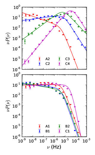
Figure 7: Smoothed PSDs ($P(\nu)$) resulting from the mock observations of the $2-10$ keV X-ray flux variations for different models. The top panel shows the results obtained for models A2 (red), C2 (blue), C3 (green), and C4 (magenta), respectively; the bottom panel shows the results obtained for models A1 (red), B1 (blue), B2 (green), and C1 (magenta), respectively. The error bars associated with each data point show the Poisson errors due to the limited number of points in each logarithmic frequency bin. The solid lines with different colors represent the best fit of a double power law to the points of each model (see Eq. 29). The model results are independent of the viewing angle $\theta_{\rm LOS}$. The PSD indicates a breaking power-law distribution. See Section 4.

The PSD is a powerful tool to investigate the nature of the flux variation at a given band for AGNs and X-ray binaries (e.g., Uttley et al., 2002; Markowitz et al., 2003; González-Martín & Vaughan, 2012; Cui et al., 1997). In this section, we investigate the dependence of the PSD extracted from the mock variations of $L_{\rm X}$ and $N_{\rm H,eff}$ on the model parameters listed in Table 1. For a given variation curve of the ‘observed’ $2-10$ keV X-ray flux or $N_{\rm H,eff}$, we first obtain its discrete Fourier transform, $F(\nu)$. Given the total observational duration $T_{\rm tot}$ and the sampling interval $\delta t$, then the total number of the data points is $N=T_{\rm tot}/\delta t$. The frequencies have $N/2$ discrete values, i.e., $\nu_{j}=j/T_{\rm tot}$ with $j=1,2,...N/2$. The normalized PSD of the variation curve can then be obtained by

$$P(\nu_{j})=\frac{2T_{\rm tot}}{\sigma^{2}N^{2}}\left|F(\nu_{j})\right|^{2},\quad(j=1,...,N/2),$$ (28)

where $\sigma$ is the variance of the curve with substantially large $T_{\rm tot}$ and small $\delta t$, i.e., $\sigma^{2}=\displaystyle{\frac{1}{N}\sum^{N}_{i=1}}(L_{{\rm X}}(t_{i})-\langle L_{\rm X}\rangle)^{2}$, $t_{i}$ represents the time at the $i$th time interval, and $\langle L_{\rm X}\rangle=\displaystyle{\frac{1}{N}\sum^{N}_{i=1}}L_{{\rm X}}(t_{i})$ is the mean. Note that the normalized PSD defined above is slightly different from those PSDs adopted in the literature (denoted by $P^{\prime}(\nu)$), with $P^{\prime}(\nu)=\frac{2T_{\rm tot}}{\mu^{2}N^{2}}\left|F(\nu)\right|^{2}=\frac{\sigma^{2}}{\mu^{2}}P(\nu)$, where $\mu=\langle L_{\rm X}\rangle$ (e.g., Markowitz et al., 2003; Uttley et al., 2002). With the definition in Equation (28), the PSDs resulting from different variation curves all satisfy $\int P(\nu)d\nu=1$, which enables us to focus on the PSD shape without involving other complexities caused by the variations as discussed later in Section 4.3.

The $P(\nu)$ directly estimated from Equation (28) contains a total number of $N/2\sim 10^{7}$ points and is usually noisy. To reduce the noise, we divide the logarithm of the frequency $\nu$ into $20$ bins with an equal logarithmic interval $\delta\log\nu$, and in each bin of $\log\nu_{k}-\delta\log\nu/2\rightarrow\log\nu_{k}+\delta\log\nu/2$ ($k=1,2,...20$), we set $P(\log\nu_{k})$ to be the mean value within this frequency bin. In Section 4.1, we fit the shape of the PSD mainly in the range of $\nu$ from $3/T_{{\rm tot}}$ to $1/(6\delta t)$. We find that the PSDs resulting from those models listed in Table 1 can be approximately described by a double power law, typically within the frequency range from $\sim 10^{-3}$ to $10^{-9}$ Hz, as shown in Figure 7. At the low-frequency end, i.e., $\nu\ll 10^{-9}$ Hz, the PSDs drop sharply, mainly due to the cutoff of the distribution of clouds at an outer boundary $a_{\rm c,max}$; at the high-frequency end, i.e., $\nu\gtrsim 10^{-3}$ Hz, the PSDs may fluctuate if the time interval of the measurements $\delta t$ is not sufficiently small. We do not include the sharply dropping part of the PSDs at low frequencies and the fluctuating part at high frequencies when using a double power-law form to fit the PSDs below.

4.1 The Shape of the Power Spectrum Density

In the absorption scenario presented above, the shape of the PSD contains the information on the spatial distribution and the intrinsic properties of the eclipsing clouds and their parent population. We choose the following double power-law form to describe the PSD shapes of the X-ray flux variations resulting from the models listed in Table 1, i.e.,

$$P(\nu)=A\left(\frac{\nu}{\nu_{\rm B}}\right)^{\gamma_{\rm l}}\left[1+\left(\frac{\nu}{\nu_{\rm B}}\right)^{2}\right]^{(\gamma_{\rm h}-\gamma_{\rm l})/2},$$ (29)

where $A$ is the normalization of the PSD, $\gamma_{\rm l}$ and $\gamma_{\rm h}$ are the slopes of the PSD at the low frequencies and the high frequencies, respectively, and $\nu_{\rm B}$ is the break frequency at the turning point. The break timescale, corresponding to the break frequency, is defined as $T^{L_{\rm X}}_{\rm B}\equiv 1/\nu_{\rm B}$. Similarly, the PSDs for the absorption column density $N_{\rm H,eff}$ variations can also be fitted by a double power-law function, the same as that shown by Equation (29); and for these cases we denote the slopes at the low frequencies and the high frequencies by $\beta_{\rm l}$ and $\beta_{\rm h}$, respectively, and the break timescale by $T_{\rm B}^{N_{\rm H}}\equiv 1/\nu_{\rm B}$.

The best-fit values of $\gamma_{\rm l}$, $\gamma_{\rm h}$, and $T^{L_{\rm X}}_{\rm B}$ (or $\beta_{\rm l}$, $\beta_{\rm h}$, and $T^{N_{\rm H}}_{\rm B}$) for those PSDs resulting from the mock observations for different models are listed in Table 1. We find that the PSD shapes are independent of $\langle N\rangle_{\rm LOS}$, if the absorption column density is in the range of $10^{21}-10^{24}{\rm cm}^{-2}$. Figure 7 shows the PSDs obtained from the mock observations for models A2, C2, C3, and C4 (top panel), and models A1, B1, B2, and C1 (bottom panel), respectively. Our calculations show that the PSD shapes resulting from the mock observations on the X-ray flux and those from the absorption column density are quite similar (see the best-fit values for the PSD shapes in Table 1). We find that such a similarity remains if the effective absorption column density is in the range of $10^{21}-10^{24}{\rm cm}^{-2}$, in which the mock X-ray flux is sensitive to the variation of $N_{\rm H,eff}$. Note that the sizes and the hydrogen densities of those eclipsing clouds with the same semimajor axis $a_{\rm c}$ are probably not exactly the same, which is not considered in our calculations. If considering the scatters of those model parameters, then the resulting PSDs near the break frequency should be smoothed slightly, and therefore the break frequency and the power-law slopes at both the high and the low-frequency ends may also change slightly, compared with those obtained without considering the scatters of the sizes and hydrogen densities.

A number of studies based on the PSD analysis of the X-ray variations suggested that the PSDs of AGNs have a slope of $\gamma_{\rm l}\sim-1$ at the low frequencies and $-4<\gamma_{\rm h}\leq-2$ at the high frequencies (e.g., Markowitz et al., 2003; Uttley et al., 2002; González-Martín & Vaughan, 2012). According to Table 1, models A1, B1, B2, C1, and C2 can produce PSDs similar to the observational ones. Those models with less column density variations caused by the clumps in torus, e.g., model C3 (or C4), result in $\gamma_{\rm l}=-0.2$ (or $0.3$ ), inconsistent with observations. Since the X-ray variations in some AGNs, e.g., NGC 1365 (e.g. Risaliti et al., 1999), NGC 7582 (e.g. Risaliti et al., 2002), and NGC 4151 (Schurch & Warwick, 2002; Markowitz et al., 2014), are probably dominated by the absorption of eclipsing clouds, therefore, the observationally determined $\gamma_{\rm l}\sim-1$ at the low frequencies (corresponding to long timescales) for the AGN PSDs may support the scenario in which the eclipsing due to the clumps in the dusty torus plays an important role in the column density and flux variations. In principle, the observational measurements on the PSDs of AGNs can put strong constraints on the spatial distribution and intrinsic properties of the eclipsing clouds and their parent population, which may be obtained by future X-ray observations and missions.

The X-ray flux variation resulting from any of the models listed in Table 1 is dominated by those eclipsing events with $b\sim 0$, which lead to relatively larger column density variations. If the X-ray variation is mainly contributed by eclipsing clouds with the same $a_{\rm c}$, then the corresponding PSD approximately peaks at a frequency $\sim\nu^{\prime}_{\rm E}(a_{\rm c})\equiv 1/t^{\prime}_{\rm E}(a_{\rm c})$. Here $t^{\prime}_{\rm E}(a_{\rm c})$ is the maximum eclipsing time of the clouds with semimajor axes $a_{\rm c}$, which is given by Equation (20). Figure 8 shows the PSD derived from the mock X-ray flux variations due to eclipses by clouds with the same semimajor axes, i.e., $a_{\rm c}=10^{2}$, $10^{3}$, $5\times 10^{3}$, and $10^{4}\,r_{\rm g}$, respectively. As seen from this figure, our numerical results demonstrate that the PSDs do peak at $\nu\sim 1/t^{\prime}_{\rm E}(a_{\rm c})$.

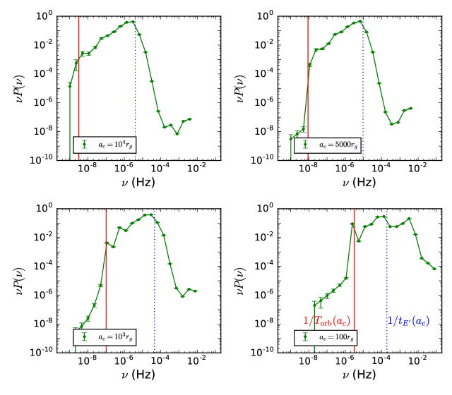
Figure 8: The PSDs [$P(\nu)$] resulting from a model in which all the clouds are set to have the same semimajor axis and all the other model parameters are similar to those in model C2. The semimajor axes of the clouds are $10^{4}r_{\rm g}$ (top-left panel), $5\times 10^{3}r_{\rm g}$ (top-right panel), $10^{3}r_{\rm g}$ (bottom-left panel), or $10^{2}r_{\rm g}$ (bottom-right panel), as labeled in each panel. The error bars associated with each data point show the Poisson errors due to the limited number of points in each logarithmic frequency bin. The vertical red solid line and the blue dotted line in each panel mark the positions of $\nu=1/T_{\rm orb}(a_{\rm c})$ and $\nu=1/t_{\rm E^{\prime}}(a_{\rm c})$, respectively, where $T_{\rm orb}(a_{\rm c})$ is the orbital period of a cloud with semimajor axis of $a_{\rm c}$, and $t_{\rm E^{\prime}}(a_{\rm c})$ is the maximum eclipsing timescale given by Equation (20). This figure illustrates that the break shown in the PSD $P(\nu)$ is dominated by the characteristic timescales $t_{\rm E^{\prime}}(a_{\rm c})$ and $T_{\rm orb}(a_{\rm c})$. See Section 4.1.1.

If the PSD of the X-ray variation is contributed by eclipsing clouds with various $a_{\rm c}$, the magnitude of the PSD at a given frequency $\nu$ then approximately corresponds to the X-ray variation contributed from those eclipsing clouds at $a_{\rm c}=t_{\rm E^{\prime}}^{-1}(1/\nu)$ (here $t_{\rm E^{\prime}}^{-1}$ is the inverse function of $t_{\rm E^{\prime}}$). Therefore, the PSD at low frequencies is determined by the eclipsing clouds at the outer region, while at high frequencies it is determined by the clouds at the inner region. The detailed dependence of the shape of the PSD (i.e., a double power-law shape described by $T_{\rm B}$, $\gamma_{\rm l}$, and $\gamma_{\rm h}$) on the model parameters is discussed as follows.

4.1.1 The Break Timescale $T_{\rm B}$

Table 1 lists the break timescale corresponding to the break frequency $\nu_{\rm B}$ of the PSDs for the mock X-ray variations ($T_{\rm B}^{L_{X}}$) and also those for the mock column density variations ($T_{\rm B}^{N_{\rm H}}$) resulting from different models. Assuming that the mass of the central MBH is $10^{7}M_{\odot}$, the break timescale $T_{\rm B}^{L_{\rm X}}$ obtained from different models range from $0.3$ to $3$ days, which appears roughly consistent with the observations (Markowitz et al., 2003; McHardy et al., 2006; González-Martín & Vaughan, 2012).

Since the PSD at the low (or high) frequencies is mainly determined by the clouds at the outer (or inner) region, the shape of the PSD due to absorption may be bent over at several frequencies due to the existence of the following characteristic scales.

• The break radius $r_{\rm t}$ in the spatial distribution of the clouds (Eq. 23): if $\alpha_{a_{\rm c},1}\neq\alpha_{a_{\rm c},2}$, the radial distribution of those eclipsing clouds in the region inside $r_{\rm t}$ is different from that in the region outside $r_{\rm t}$.

• The inner boundary for the spatial distribution of the eclipsing clouds, i.e., $a_{\rm c,min}>0$: no eclipsing clouds exist within $a_{\rm c,min}$, and therefore, the PSD drops rapidly at frequencies $\nu\gtrsim 1/t_{\rm E^{\prime}}(a_{\rm c,min})$.

• The characteristic semimajor axis $a_{\rm eq}$ at which the cloud size $R_{\rm c}$ is equal to the X-ray source size $R_{\rm X}$: for an eclipsing cloud with $a_{\rm c}<a_{\rm eq}$ and $R_{\rm c}\lesssim R_{\rm X}$, the resulting absorption column density approximately follows $N_{\rm H}\propto R_{\rm c}^{3}/R_{\rm X}^{2}$; while for an eclipsing cloud with $a_{\rm c}\gg a_{\rm eq}$ and $R_{\rm c}(a_{\rm c})\gg R_{c}(a_{\rm eq})$, the column density approximately follows $N_{\rm H}\propto R_{\rm c}$. The dependence of $N_{\rm H}$ on $R_{\rm c}$ changes smoothly around $a_{\rm eq}$. According to our numerical results, we find that the turning points of the PSD are around $\nu\sim 1/t_{\rm E^{\prime}}(a_{\rm eq})$, where $a_{\rm eq}=R_{\rm c}^{-1}(\xi R_{\rm X})=a_{\rm c,min}(\xi R_{\rm X}/R_{\rm c,0})^{1/\alpha_{R_{\rm c}}}$, and $\xi$ is slightly model-dependent. For model C1, we have $\xi\simeq 1.7$. For other models listed in Table 1, we have $\xi\sim 0.3-2.0$. If $R_{\rm c,0}<\xi R_{\rm X}$, we have $a_{\rm eq}\geq a_{\rm c,min}$. However, $a_{\rm eq}$ does not exist if $R_{\rm c,0}>\xi R_{\rm X}$.

We find that the resulting PSDs from those models listed in Table 1 bend over slightly near $\nu_{\rm E^{\prime}}(r_{\rm t})=1/t_{\rm E^{\prime}}(r_{\rm t})$ if $\alpha_{a_{\rm c},1}\neq\alpha_{a_{\rm c},2}$. For those models listed in Table 1, we have $\nu_{\rm E^{\prime}}(r_{\rm t})\ll\nu_{\rm B}$. Our model results show that this bending of the PSDs around $\nu_{\rm E^{\prime}}(r_{\rm t})$ is not significant compared with that near $\nu_{\rm B}=1/T_{\rm B}$. The main reason is that the difference between $\alpha_{a_{\rm c},1}$ and $\alpha_{a_{\rm c},2}$ is only moderate. However, the radial distributions of eclipsing clouds for models with extremely large differences between $\alpha_{a_{\rm c},1}$ and $\alpha_{a_{\rm c},2}$ are usually unphysical. For example, the cases with clouds extremely abundant at the outer region of the dusty torus while no clouds are in the BLR, or vice versa, are inconsistent with observations and the unification model for AGNs.

We find that the resulting PSDs break significantly near $\nu_{\rm E^{\prime}}(a_{\rm c,min})=1/t_{\rm E^{\prime}}(a_{\rm c,min})$ due to the existence of an inner boundary ($a_{\rm c,min}$) for the cloud spatial distribution, or near $\nu_{\rm E^{\prime}}(a_{\rm eq})=1/t_{\rm E^{\prime}}(a_{\rm eq})$ due to the existence of the characteristic scale $a_{\rm eq}$. If both $a_{\rm c,min}$ and $a_{\rm eq}$ exist, then the break frequency $\nu_{\rm B}$ obtained from the fitting to the PSDs is roughly given by the one with a smaller value, i.e.,

$$\nu_{\rm B}\sim{\rm min}[\nu_{\rm E^{\prime}}(a_{\rm c,min}),\nu_{\rm E^{\prime}}(a_{\rm eq})],$$ (30)

which appears as the first significant break in the PSDs with $\nu>10^{-8}$ Hz, while the higher frequency one indicates a further decrease of the PSD magnitude at frequencies $\nu>\nu_{\rm B}$ (the slope of those PSDs at higher frequencies becomes steeper). Figure 9 illustrates the dependence of the break frequency $\nu_{\rm B}$ and the break timescale $T_{\rm B}$ on $R_{\rm X}$, $a_{\rm c,min}$, and $\alpha_{R_{\rm c}}$, as suggested by Equation (30). As seen from this figure, $T_{\rm B}$ increases with increasing the inner boundary of the radial distribution of the eclipsing clouds ($a_{c,\rm min}$, top-left panel), or with increasing the source sizes ($R_{\rm X}$, bottom-left panel). The right panels of this figure show that $T_{\rm B}$ increases from $\sim 1$ day to $2$ days when $a_{\rm c,min}$ increases from $100r_{\rm g}$ to $10^{4}r_{\rm g}$, and $T_{\rm B}$ increases from $\sim 1$ day up to $\sim 4$ days when $R_{\rm X}$ increases from $5r_{\rm g}$ to $15r_{\rm g}$. These results are well consistent with the predictions by Equation (30).

The PSDs obtained from our models usually turn over smoothly around the break frequency $\nu_{\rm B}$. However, the PSDs obtained from observations are sometimes limited by the total observational duration ($T_{\rm tot}$) at the lowest frequency ($\nu_{\rm min}\sim 1/T_{\rm tot}$) and the minimum sampling interval ($\delta t$) at the highest frequency ($\nu_{\rm max}\sim 1/(2\delta t)$). If $\nu_{\rm min}$ (or $\nu_{\rm max}$) is close to $\nu_{\rm B}$, then the $\gamma_{\rm l}$ (or $\gamma_{\rm h}$) and $\nu_{\rm B}$ obtained from the best fits to the PSDs are biased. It is important to perform observations with a sufficiently long period and a sufficiently small time interval in order to estimate the shape of the PSD for the X-ray variation of an AGN accurately.

Note that the existence of the outer boundary for the spatial distribution of those eclipsing clouds may also lead to a break in the PSD. This break, however, corresponds to a timescale of $\gg 10$ years, which is probably difficult to probe in the near future.

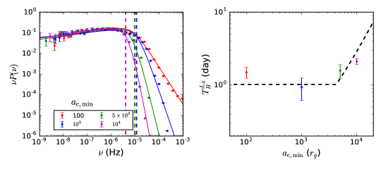
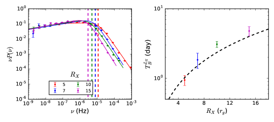
Figure 9: Top-left panel: the PSDs resulting from model C2 and three other models with parameters similar to those in model C2 except for a different value of the inner boundary of the spatial distribution of those clouds as labeled in the figure ($a_{\rm c,min}=10^{3}$, $5\times 10^{3}$, and $10^{4}r_{\rm g}$, respectively). The vertical red dashed line overlaps with the vertical blue dashed line in this panel. Top-right panel: the break timescales obtained from the fittings to the PSDs shown in the top-left panel. Bottom-left panel: the PSDs resulting from model C2 and three other models with parameters similar to those in model C2 except for a different value for the size of the X-ray source as labeled in the figure ($R_{\rm X}=7$, $10$, and $15r_{\rm g}$, respectively). Bottom-right panel: the break timescales obtained from the fittings to the PSDs shown in the bottom-left panel. The solid lines in the left panels represent the best fits to the PSDs. The vertical dashed lines in the left panels represent the estimates obtained from Equation (30). The black dashed curves in the right panels represent the estimates obtained from Equation (30). The simulation results are consistent with Equation (30) well, which suggests that the break frequency in the PSD is mainly affected by the clouds with semimajor axis $a_{c}\sim{\rm max}(a_{c,{\rm min}},a_{\rm eq})$. See Section 4.1.1.

4.1.2 The PSD Shape at Low Frequencies: $\gamma_{l}$

The slope of the PSD at frequencies $<\nu_{\rm B}$ is mainly determined by the spatial distribution and the intrinsic properties of the eclipsing clouds at the outer region, i.e., the dusty torus. If the clouds at the outer region in a model have relatively larger sizes (larger $\alpha_{R_{\rm c}}$) and hydrogen densities (larger $\alpha_{n_{\rm H}}$), or they are more abundant, compared with those in another model, then the PSD slope at low frequencies ($\gamma_{\rm l}$ or $\beta_{\rm l}$) resulting from this model should be steeper (smaller) than those from the other model. For example, $\gamma_{\rm l}$ resulting from the model A2 is smaller than that from model A1 simply because the hydrogen densities of the clouds in the dusty torus region in model A2 are relatively larger compared with those in model A1. Similarly, $\gamma_{\rm l}$ resulting from model C3 or C4 is larger than that from model C2 because the hydrogen densities of the eclipsing clouds at the outer region in model C3 are relatively smaller than those in model C2 or the sizes of those clouds in model C4 are relatively smaller than those in model C2. As seen from Figure 7, the magnitude of the PSD at lower frequencies resulting from model B1 is slightly larger than that from model C1 (smaller $\gamma_{\rm l}$) because there are relatively more clouds distributed at the outer region in model B1 than those in model C1. Increasing the value of $\alpha_{R_{\rm c}}$, $\alpha_{n_{\rm H}}$, $\alpha_{a_{\rm c},2}$, $\lambda_{\rm Edd}$, or $r_{\rm t}$, the contributions from those eclipsing clouds at large distance to the central MBH to the PSD increases correspondingly, which results in a smaller $\gamma_{\rm l}$. As an example, for model C2, $\gamma_{\rm l}$ decreases from $\sim-0.8$ to $-1.2$ if $r_{\rm t}/r_{\rm d}$ increases from $0.01$ to $1$; while $\gamma_{\rm l}$ decreases from $\sim 0.3$ to $\sim-1.3$ if $\alpha_{R_{\rm c}}$ increases from $0.5$ to $1.2$; for model C1, $\gamma_{\rm l}$ decreases from $-0.2$ to $-1.4$ if $\alpha_{n_{\rm H}}$ increases from $-2.5$ to $1.0$; while $\gamma_{\rm l}$ decreases from $-0.8$ to $-1.2$ if $\lambda_{\rm Edd}$ increases from $0.01$ to $1$. We find that the dependence of $\gamma_{\rm l}$ on other parameters, i.e., $R_{\rm X}$, $a_{\rm c,min}$, and $\alpha_{a_{\rm c},1}$, is little (see Fig. 9).

Note also that the $\gamma_{\rm l}$ and $\gamma_{\rm h}$ of PSDs are independent of $n_{\rm H,0}$ if the column density $N_{\rm H}$ ranges from $10^{21}$ to $10^{24}{\rm cm}^{-2}$, as the increase of $n_{\rm H,0}$ enhances the contribution to the PSDs at both low and high frequencies simultaneously.

4.1.3 The PSD Shape at High Frequencies: $\gamma_{\rm h}$

The magnitude of the resulting PSD at high frequencies, usually above $10^{-5}-10^{-4}$ Hz for an MBH with mass $10^{7}M_{\odot}$, is mainly determined by the eclipsing clouds (e.g., the BLR clouds) at close distances to the MBH. If the eclipsing clouds at the inner region in a model have relatively larger sizes and densities, or if they are more abundant at small $a_{\rm c}$, compared with those in another model, then the magnitude of the resulting PSD (not the slope) at high frequencies is larger compared with the other model. As discussed in Section 4.1.1, the steep bending-down of the PSD at high frequencies is mainly due to the lack of eclipsing clouds within $a_{\rm c,min}$ and the less significant absorption due to those clouds with smaller $a_{\rm c}$ because of their smaller size and consequently smaller absorption column densities ($N_{\rm H}\propto R_{\rm c}^{3}(a_{\rm c})/R_{\rm X}^{2}$). The steep slope of the PSD at high frequencies $\gamma_{\rm h}$ thus indicates the degree of the lack of those eclipsing events with small distances to the MBH (or small $a_{\rm c}$). We find that $\gamma_{\rm h}$ mainly depends on $a_{\rm c,min}$ and the index $\alpha_{R_{\rm c}}$ describing the size change of the eclipsing clouds with the semimajor axis. As shown in Figure 9, for a larger inner boundary ($a_{\rm c,min}$) of the cloud distribution, the slope of the PSD at high frequencies is steeper. The $\alpha_{a_{\rm c},1}$ affects the value of $\gamma_{\rm h}$. Decreasing $\alpha_{a_{\rm c},1}$ increases the magnitude of the PSD at frequencies higher than the break frequency and lower than $\nu_{\rm E^{\prime}}(a_{\rm c,min})$ (e.g., see the PSDs of models A1 and C1 in the frequency range $\sim 10^{-5}-10^{-3}$ Hz in Fig. 7), which may lead to a smaller $\gamma_{h}$ in the double power-law fit to the PSD if $a_{\rm min}$ is only several times smaller than $a_{\rm eq}$ as in the case for model C1. As seen from Figure 7, $\gamma_{h}$ in model C1 is steeper than that in model A1, although $\alpha_{a_{\rm c},1}$ in model C1 is relatively smaller, which is because no clouds are set within the inner boundary $a_{\rm c,min}=10^{3}r_{g}$ and the decrease of $\alpha_{a_{\rm c},1}$ leads to a larger change between the numbers of the clouds contributing to the PSD at $\nu\sim 10^{-5}-10^{-4}$ Hz and those contributing to the PSD at higher frequencies. If $a_{\rm min}\ll a_{\rm eq}$, decreasing $\alpha_{a_{\rm c},1}$ may increase the slope of $\gamma_{h}$ within the frequency range $\nu_{\rm E^{\prime}}(a_{\rm eq})\lesssim\nu\ll\nu_{\rm E^{\prime}}(a_{\rm c,min})$. If $a_{\rm min}>a_{\rm eq}$, the dependence of $\gamma_{h}$ on $\alpha_{a_{\rm c},1}$ is weak. The $\gamma_{\rm h}$ also depends on $\alpha_{n_{\rm H}}$ (models C2 and C3). The $\gamma_{\rm h}$ is insensitive to $\lambda_{\rm Edd}$ and $r_{t}$, as $\nu_{\rm E^{\prime}}(r_{\rm t})\ll\nu_{\rm B}$. The value of $R_{X}$ may affect the position of $\nu_{B}$, but not $\gamma_{\rm h}$.

4.2 The Relationship between $T_{\rm B}$ and $M_{\bullet}$

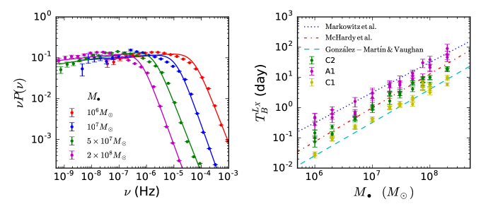
Figure 10: Left: the PSDs resulting from model C2 by setting four different values for the MBH mass and the best fits to them. This panel shows that the shape of the PSD is insensitive to the MBH mass except that the location of the break frequency decreases with increasing MBH mass. Right: the break timescale $T_{\rm B}^{L_{\rm X}}$ as a function of the MBH mass $M_{\bullet}$. The green, magenta, and yellow circles represent the results obtained from models C2, A1, and C1, respectively. The error bars associated with each point represent the $1-\sigma$ error of the best fit. For each model, we adopt various values for the mass of the central MBH in the range from $10^{6}$ to $2\times 10^{8}M_{\odot}$. For each given MBH mass, the results obtained for those cases with three different view angles, i.e., $\theta_{\rm LOS}=75^{{}^{\circ}},60^{{}^{\circ}}$, and $45^{{}^{\circ}}$, are shown for each model. The blue dotted line, the red dash-dotted line, and the cyan dashed line represent the observational fitting results given by Markowitz et al. (2003), McHardy et al. (2006), and González-Martín & Vaughan (2012), respectively. This figure shows that the absorption scenario for the AGN X-ray variations naturally leads to a strong correlation between $T_{\rm B}^{L_{\rm X}}$ and $M_{\bullet}$, which can be consistent with the relationship obtained from observations. See Section 4.2.

A number of observations suggest that the break timescales $T_{\rm B}^{L_{\rm X}}$ obtained from the PSDs of the AGN X-ray variations correlate with the masses of the central MBHs. For example, Markowitz et al. (2003) found a linear correlation between these two quantities as $T_{\rm B}^{L_{\rm X}}/{\rm day}=M_{\bullet}/10^{6.5}M_{\odot}$; McHardy et al. (2006) confirmed the correlation between $T_{\rm B}$ and $M_{\bullet}$, and they further suggested that the accretion rate should also be included in the relationship, i.e., $\log(T_{\rm B}^{L_{\rm X}}/{\rm day)}=2.1\log(M_{\bullet}/10^{6}M_{\odot})-0.98\log(L_{\rm bol}/10^{44}{\rm erg~{}s}^{-1})-2.3$, where $L_{\rm bol}$ is the bolometric luminosity; González-Martín & Vaughan (2012) recently obtained a similar relationship, i.e., $\log(T_{\rm B}^{L_{\rm X}}/{\rm day)}=1.34\log(M_{\bullet}/10^{6}M_{\odot})-0.24\log(L_{\rm bol}/10^{44}~{}{\rm erg~{}s}^{-1})-1.9$, of which the dependence on the accretion rate is subsequently weaker compared with that in McHardy et al. (2006).

To study the scaling relation between $T_{\rm B}^{L_{\rm X}}$ and $M_{\bullet}$ in the absorption scenario for the X-ray variations, we perform more simulations for those models with the same settings as models A1, C1, and C2, respectively, except for adopting various masses for the central MBH in the range from $10^{6}$ to $2\times 10^{8}M_{\odot}$. (For other models, we obtain the similar conclusions.) We find that the shape of the PSD is independent of the setting for the hydrogen densities of those clouds with semimajor axis of $a_{\rm c,min}$ (i.e., $n_{\rm H,M_{\bullet},0}$) if the absorption column density is in the range from $\sim 10^{21}$ to $10^{24}~{}{\rm cm}^{-2}$. Therefore, we simply set $n_{\rm H,M_{\bullet},0}=n_{\rm H,0}(10^{7}M_{\odot}/M_{\bullet})$, where $n_{\rm H,0}$ is the initial setting for those cases with $M_{\bullet}=10^{7}M_{\odot}$ as listed in Table 1. With this setting, those cases with too many Compton-thick clouds are avoided. Alternatively setting an $n_{\rm H,0}$ a few times larger, or smaller, for those models listed in Table 1, does not significantly affected the model results.

Figure 10 shows our model results on $T_{\rm B}^{L_{\rm X}}$ as a function of $M_{\bullet}$. As seen from the figure, the absorption scenario for the AGN X-ray variations naturally leads to a strong correlation between $T_{\rm B}^{L_{\rm X}}$ and $M_{\bullet}$, which can be consistent with the relationship obtained from observations. The scatters in the spatial distribution and the intrinsic properties of the eclipsing clouds among individual AGNs, indicated by the different model settings listed in Table 1, and those shown in Figure 9, may lead to a scatter in the relationship as shown in Figure 10.

The rough consistency between the observations and our model results suggests that the absorption model, i.e., that the AGN X-ray variations are mainly caused by those eclipsing clouds crossing the LOS, may provide a natural explanation to the shapes of the PSDs for some, if not all, AGNs and the scaling relation between the break timescales and the MBH masses for those AGNs. In principle, a comparison between the $T^{L_{\rm X}}_{\rm B}-M_{\bullet}$ relation resulting from those absorption models and the observational ones may put strong constraints on the model parameters. However, it appears there are large uncertainties in the observationally estimated $T^{L_{\rm X}}_{\rm B}-M_{\bullet}$ relation (as large as $1$ dex), which prevent a detailed statistical comparison of the model results with the observational ones.

For those absorption models with the same settings on the spatial distribution and the intrinsic properties of the clouds but with different masses of the central MBH, we find that the slopes of the resulting PSDs at both the low frequencies ($\gamma_{\rm l}$) and the high frequencies ($\gamma_{\rm h}$) are independent of the MBH mass (see the right panel of Figure 10). No strong dependence of the scaling relation on the Eddington ratio is found for the models studied in this paper because only one model parameter, $r_{\rm t}$, is set to correlate with the Eddington ratio.

Note here that in the absorption scenario a correlation between $T^{L_{\rm X}}_{\rm B}$ and $M_{\bullet}$ with a slope of about 1 or $1+\frac{1}{2}(\alpha_{R_{\rm c}}^{-1}-1)$ in the log-log space can be produced if $R_{\rm X}$ and $a_{\rm c,min}$ scale linearly with the MBH mass $M_{\bullet}$. It is plausible that $R_{\rm X}$ and $a_{\rm c,min}$ scale linearly with the MBH mass $M_{\bullet}$, since the intrinsic properties of the clouds and the spatial distribution of those clouds probably scale with the luminosity of an AGN, which is proportional to the Eddington luminosity and thus linearly scales with the MBH mass. In reality, it is possible that other parameters, e.g., the cloud radius $R_{\rm c}$ and the inner boundary for the spatial distribution of eclipsing clouds $a_{\rm c,min}$, are correlated with the Eddington ratio and consequently the break timescale (or frequency) also depends on the Eddington ratio. Since the relationships between these parameters and the Eddington ratio are not clear, a further exploration of the dependence of the scaling relation on the Eddington ratios is beyond the scope of the paper.

4.3 On the Amplitude of the Variation

The variation of the X-ray emission from an AGN can be quantified by the normalized excess variance (NEV)

$$\sigma_{{\rm NEV},L}^{2}=\frac{\displaystyle{\sum^{N}_{i=1}}(L_{{\rm X}}(t_{i})-\langle L_{\rm X}\rangle)^{2}}{N\langle L_{\rm X}\rangle^{2}}.$$ (31)

If the variation of the X-ray emission of some AGNs is mainly due to the absorption by eclipsing clouds as assumed in this paper, the NEV ($\sigma_{{\rm NEV},L}$) for those models listed in Table 1 can be obtained from our simulations. Similarly, the NEV of the absorption column density $\sigma_{{\rm NEV},N_{\rm H}}$ can be obtained by replacing $L_{\rm X}(t_{i})$ and $\langle L_{\rm X}\rangle$ by $N_{\rm H}(t_{i})$ and $\langle N_{\rm H}\rangle$ in Equation (31), respectively, and $N_{\rm H}(t_{i})$ are obtained from the mock observations at the $i$-th time interval. The actual value of $\sigma_{\text{NEV},L}^{2}$ depends on the total observational time $T_{\text{tot}}$ and the duration of the observational time interval $\delta t$. If $T_{\text{tot}}$ is not sufficiently large, then those eclipses caused by clouds with large $a_{\text{c}}$ cannot be fully counted, and if $\delta t$ is too large, then those eclipsing clouds with small $a_{\text{c}}$ are also not fully counted.

We assume that the AGN X-ray variations for different AGNs follow an intrinsic PSD with the following universal double power-law form, i.e.,

$$P(\nu)\simeq\begin{cases}A\left(\frac{\nu}{\nu_{\rm B}}\right)^{\gamma_{\rm h}},\quad\text{when }\nu\geq\nu_{\rm B},\\ A\left(\frac{\nu}{\nu_{\rm B}}\right)^{\gamma_{\rm l}},\quad\text{when }\nu<\nu_{\rm B}\\ \end{cases}$$ (32)

as a simplified form of Equation (29), where $A$ is the amplitude of the PSD at $\nu_{\rm B}$, $\gamma_{\text{h}}<\gamma_{\text{l}}$, and $\gamma_{\text{h}}<-1$. If the frequency range limited by “observations” is from $\nu_{\rm min}\sim 1/T_{\rm tot}$ to $\nu_{\text{max}}\sim 1/(2\delta t)$ (which is substantially narrower than the range considered in the models), and $\nu_{\text{min}}\ll\nu_{\text{max}}$, then the NEV estimated from the observations can be approximately given by

$$\sigma^{2}_{\text{NEV},L}\simeq\int^{\nu_{\text{max}}}_{\nu_{\text{min}}}\delta_{L}^{2}P(\nu)d\nu=\delta_{L}^{2}\frac{A\nu_{\text{B}}}{\gamma_{\text{h}}+1}\times$$

$$\begin{cases}\left[\left(\frac{\nu_{\text{max}}}{\nu_{\text{B}}}\right)^{\gamma_{\text{h}}+1}-\left(\frac{\nu_{\text{min}}}{\nu_{\text{B}}}\right)^{\gamma_{\text{h}}+1}\right],\\ ~{}~{}~{}~{}~{}~{}~{}~{}~{}~{}~{}~{}~{}~{}~{}~{}~{}~{}~{}~{}~{}~{}~{}~{}~{}~{}~{}~{}~{}~{}~{}~{}~{}~{}~{}~{}~{}~{}~{}~{}\text{when }\nu_{\text{min}}\geq\nu_{\text{B}};\\ \left[\left(\frac{\nu_{\text{max}}}{\nu_{\text{B}}}\right)^{\gamma_{\text{h}}+1}-1\right]+\frac{\gamma_{\text{h}}+1}{\gamma_{\text{l}}+1}\left[1-\left(\frac{\nu_{\text{min}}}{\nu_{\text{B}}}\right)^{\gamma_{\text{l}}+1}\right],\\ ~{}~{}~{}~{}~{}~{}~{}~{}~{}~{}~{}~{}~{}~{}~{}~{}~{}~{}~{}~{}~{}~{}~{}~{}~{}~{}~{}~{}~{}~{}~{}~{}~{}~{}~{}~{}~{}~{}~{}~{}\text{when }\nu_{\text{min}}<\nu_{\text{B}}<\nu_{\text{max}};\\ \frac{\gamma_{\text{h}}+1}{\gamma_{\text{l}}+1}\left[\left(\frac{\nu_{\text{max}}}{\nu_{\text{B}}}\right)^{\gamma_{\text{l}}+1}-\left(\frac{\nu_{\text{min}}}{\nu_{\text{B}}}\right)^{\gamma_{\text{l}}+1}\right],\\ ~{}~{}~{}~{}~{}~{}~{}~{}~{}~{}~{}~{}~{}~{}~{}~{}~{}~{}~{}~{}~{}~{}~{}~{}~{}~{}~{}~{}~{}~{}~{}~{}~{}~{}~{}~{}~{}~{}~{}~{}\text{when }\nu_{\text{max}}\leq\nu_{\text{B}},~{}\end{cases}$$ (33)

where $\delta_{L}^{2}\equiv\mathop{\lim}\limits_{\Delta T\rightarrow\infty}\int_{0}^{\Delta T}[1-L(t)/\overline{L(t)}]^{2}dt/\Delta T$ and $\overline{L(t)}\equiv\mathop{\lim}\limits_{\Delta T\rightarrow\infty}\int_{0}^{\Delta T}L(t)dt/\Delta T$. If $\gamma_{\text{h}}$ [or $\gamma_{\text{l}}$] equals $-1$, the terms $\left(\nu_{\text{min}}/\nu_{\text{B}}\right)^{\gamma_{\text{h}}+1}$ and $\left(\nu_{\text{max}}/\nu_{\text{B}}\right)^{\gamma_{\text{h}}+1}$ [or $\left(\nu_{\text{min}}/\nu_{\text{B}}\right)^{\gamma_{\text{l}}+1}$ and $\left(\nu_{\text{max}}/\nu_{\text{B}}\right)^{\gamma_{\text{l}}+1}$] should be replaced by $(\gamma_{\text{h}}+1)\ln\left(\nu_{\text{min}}/\nu_{\text{B}}\right)$ and $(\gamma_{\text{h}}+1)\ln\left(\nu_{\text{max}}/\nu_{\text{B}}\right)$ [or $(\gamma_{\text{l}}+1)\ln\left(\nu_{\text{min}}/\nu_{\text{B}}\right)$ and $(\gamma_{\text{l}}+1)\ln\left(\nu_{\text{max}}/\nu_{\text{B}}\right)$], respectively.

In the absorption scenario presented in this paper, the X-ray variations are due to the eclipses of clouds in the BLR and the dusty torus. As shown in Figure 10, the power at $\nu_{\text{B}}$, i.e., $A\nu_{\text{B}}$, is more or less a constant for the different BH masses of a given model and $\nu_{\text{B}}\propto M_{\bullet}^{-1}$. If $\delta_{L}^{2}$ is also constant with different $M_{\bullet}$, then $\sigma^{2}_{\text{NEV},L}\propto M_{\bullet}^{\gamma_{\text{h}}+1}$ when $\nu_{\text{min}}>\nu_{\text{B}}$, and $\sigma^{2}_{\text{NEV},L}\propto M_{\bullet}^{\gamma_{\text{l}}+1}$ when $\nu_{\text{max}}<\nu_{\text{B}}$, and transits from $\propto M_{\bullet}^{\gamma_{\text{h}}+1}$ to $\propto M_{\bullet}^{\gamma_{\text{l}}+1}$ when $\nu_{\text{B}}$ moves from $\nu_{\text{min}}$ to $\nu_{\text{max}}$. This suggests that the absorption scenario for the X-ray variations can also naturally lead to a correlation between the MBH mass and the NEV. For example, model C2 results in a PSD with $\gamma_{\text{h}}=-2.6$ and $\gamma_{\text{l}}=-0.9$, which may lead to a correlation $\sigma^{2}_{\text{NEV},L}\propto M_{\bullet}^{-1.6}$ at the high-MBH mass range and $\propto M_{\bullet}^{0.1}$ at the low-MBH mass range.

A scatter in the $\sigma^{2}_{\text{NEV}}$-$M_{\bullet}$ correlation can be caused at the least by the following factors. (1) In reality, $\delta_{L}^{2}$ may depend on the settings of the spatial distribution and the intrinsic properties of the eclipsing clouds, which could lead to a scatter in the $\sigma^{2}_{\text{NEV}}$-$M_{\bullet}$ correlation. For example, we find that $\delta_{L}^{2}\propto\left<N\right>_{\text{LOS}}$; even if the cloud size and the size of the X-ray emitting region scale linearly with the MBH mass to cancel out some dependence on the MBH mass in Eq. (LABEL:eq:nlos), it still depends on the total number of clouds $N_{\text{tot}}$ and the viewing angle. (2) The differences among the spatial distributions of the eclipsing clouds in different AGNs with the same MBH mass may result in different shapes of the PSDs (defined by $\nu_{\text{B}}$, $\gamma_{\text{h}}$ and $\gamma_{\text{l}}$), which consequently leads to a scatter to the $\nu_{\text{B}}$-$M_{\bullet}$ relation and thus further introduce scatters to the $\sigma^{2}_{\text{NEV}}$-$M_{\bullet}$ relation.

Note that a number of studies have shown that the magnitudes of the AGN X-ray variation on short timescales tightly correlate with the masses of the central MBHs (e.g., Lu & Yu, 2001b; O’Neill et al., 2005; Nikołajuk et al., 2009; Zhou et al., 2010; Ponti et al., 2012; McHardy, 2013; Soldi et al., 2014). The variation magnitudes on long timescales may saturate and become independent of the MBH masses (Shimizu & Mushotzky, 2013; Markowitz & Edelson, 2004). These observations can be well interpreted as the X-ray variations of different AGNs following a universal PSD, with a break frequency correlating with the MBH mass (Markowitz & Edelson, 2004). This relation may be a direct result of a uniform PSD with $\gamma_{\text{h}}\sim-4$—$-2$ and $\gamma_{\rm l}$ close to -1 for the X-ray variation in those AGNs as discussed intensively in the literature (e.g., Ponti et al., 2012; Ludlam et al., 2015; Pan et al., 2015).

5 Conclusions and Discussions

In this paper, we study the AGN X-ray variations due to the absorption of the clouds or clumps in the BLR and the dusty torus that happen to cross the LOS. In this absorption scenario for the AGN X-ray variations, we investigate the dependence of the power spectral densities (PSDs) of the X-ray flux and the absorption column density variations on the spatial distribution and the intrinsic properties of those clouds. We analyze various statistical properties of the X-ray eclipsing events, e.g., the event rate, the mean number of the eclipsing clouds per unit time, and the statistical distributions of the parameters for the eclipsing events. We perform Monte-Carlo simulations to realize the kinematics of those clouds in the vicinity of AGNs and obtain mock X-ray variations due to the X-ray eclipses. We find that the resulting PSDs of the X-ray flux or the absorption column density variations can be described by a breaking double power-law form in the frequency range from $10^{-3}$ Hz to $10^{-9}$ Hz, which can be well consistent with those measured from observations. The PSD at the low (or high) frequencies is mainly controlled by the spatial distribution and the intrinsic properties of the eclipsing clouds at the outer (or inner) region, presumably by some clouds in the dusty torus (or BLR).

We find that the break frequency of the PSD is roughly determined by either the eclipsing durations of those eclipsing clouds with the minimum semimajor axis (i.e., $\nu\sim 1/t_{\rm E^{\prime}}(a_{\rm c,min})$) or the eclipsing duration of those clouds with a characteristic semimajor axis ($a_{\rm eq}$, which is defined by that the sizes of the clouds with semimajor axes larger than $a_{\rm eq}$ are larger than the size of the X-ray emission region, while the sizes of the clouds with semimajor axes smaller than $a_{\rm eq}$ are smaller than the size of the X-ray emission region). We demonstrate that the break timescales, corresponding to the break frequencies of the PSDs, are strongly correlated with the masses of the central MBHs in the cloud absorption scenario for the X-ray variations of AGNs, which may provide a natural explanation to the scaling relation suggested by observations for some AGNs (Markowitz et al., 2003; McHardy et al., 2006; González-Martín & Vaughan, 2012). If future observations can more accurately determine this scaling relation, the cloud absorption scenario for the X-ray variations of AGNs may be further constrained and the underlying physics for the scaling relation may be better understood. This scaling relation is, therefore, expected to provide a robust tool to estimate the masses of MBHs in some type 2, if not all, AGNs. (Note that the popular reverberation mapping technique is not easy to apply to type 2 AGNs, for which no strong broad emission lines can be directly detected.) For some type 1 AGNs, this relation may also be applicable to estimate the masses of the central MBHs if their X-ray variations are dominated by the absorption of eclipsing clouds. We also show that this correlation, together with the assumption that the X-ray variation of different AGNs follows a universal PSD, will lead to a dependence of the X-ray variation amplitude on BH mass as shown in some observations.

The spatial distribution and the intrinsic properties of the eclipsing clouds and their parent population can be extracted from the X-ray flux variation (if it is mainly due to the absorption of eclipsing clouds), the column density variation, and the PSDs of these variations. Observations have shown that the X-ray variations of some AGNs, such as NGC 1365 (e.g. Risaliti et al., 1999), NGC 7582 (e.g. Risaliti et al., 2002) , and NGC 4151 (Schurch & Warwick, 2002; Markowitz et al., 2014), are probably dominated by the absorption of eclipsing clouds. For those AGNs, it is possible to adopt the X-ray eclipse model introduced in this study to match the PSDs of their X-ray flux variations (or the PSDs of their absorption column density variations, if available) individually. With such a modeling, robust constraints may be obtained on the spatial distribution and the intrinsic properties of the eclipsing clouds and their parent populations for those individual AGNs. The statistical scatters of the spatial distribution and the intrinsic properties of the clouds in different AGNs and its dependence on various AGN properties, such as luminosity, MBH mass, Eddington ratio, etc., may also be revealed by studying a sample of such AGNs. This may help to establish a unified theory for the nature of the BLR and the torus.

As the UV-optical sources (mainly from the accretion disk) are much more extended than the X-ray sources, it is likely that some AGNs show X-ray variations due to eclipsing clouds, while they appear as type 1 AGNs in the UV-optical band. For these objects, it will be interesting to investigate the flux variability in the UV-optical band due to the covering of the clouds together with the variation of the X-ray emission. The comparison of both the model predictions and observations in the multiple bands can help to set robust constraints on the structure and property distributions of the AGN clouds, and also the type 1 and type 2 dichotomy. Note that the covering fraction of the clouds and the variability of the flux appearing in the UV-optical band may have a different dependence on the cloud structure and properties from those in the X-ray band. A comprehensive exploration of these features, which is beyond the scope of this paper, is worthy.

In addition to X-ray flux variations, the variation of the Fe K$\alpha$ line emission due to eclipsing may also be used to probe the kinematic structure of the parent population of the eclipsing clouds and the inner disk structure.

It has been shown that the spatial distribution and the intrinsic properties of the BLR clouds and the clumps in the dusty torus can be revealed by the reverberation mapping technique (e.g., Li et al., 2013; Chelouche & Zucker, 2013; Pancoast et al., 2011, 2013). If the X-ray variations in some AGNs with broad emission lines are due to the absorption of eclipsing clouds in the BLR and/or the dusty torus, it may be possible to combine both the reverberation mapping technique and the PSD analysis of the X-ray flux (and the absorption column density) variations to study and constrain the properties of those clouds in the BLR and the dusty torus, which may help to reach a coherent understanding of various AGN emission/absorption features and the immediate environment of the central engine of AGNs.

For some AGNs, the observed X-ray flux variations may be mainly due to the changes of the properties of the inner accretion disk and the X-ray emitting corona (e.g., Lyubarskii, 1997; Lamer et al., 2003a; Uttley et al., 2002; Zdziarski et al., 2003; Poutanen & Fabian, 1999; Lu & Yu, 2001a; Fabian & Vaughan, 2003; Marinucci et al., 2014), of which the PSDs of the X-ray variations may be quite different from those obtained from the absorption scenario studied in this paper. If it is due to the flicker noise in accretion disks as suggested by Lyubarskii (1997), for example, the resulting PSD may be typically $\propto\nu^{-1}$. In the literature, however, there are no explicit predictions on the PSD of the X-ray flux variations due to the intrinsic changes for most of other proposed models. Future progress on the studies of the intrinsic variation of the X-ray emission from AGNs may provide some information on the PSD of this variation, which may be used to distinguish from the absorption scenario for the X-ray flux variation of some AGNs.

Note here that we mainly focus on the variations of the X-ray emission in the $2-10$ keV band in this paper. For the X-ray emission at a band with higher energy, e.g., $10-100$ keV, the shape of the resulting PSD is the same as that for the $2-10$ keV X-ray emission, although the amplitude of the variation at the high-energy band is substantially smaller than that at the $2-10$ keV band. The independence of the PSD shape from the energy and the dependence of the variation amplitude on the energy are the simple nature of the absorption scenario for the X-ray variations, which may be used to distinguish the absorption scenario from those models assuming intrinsic variations (e.g., Miller et al., 2008).

References

- Abrassart & Czerny (2000) Abrassart, A., & Czerny, B. 2000, A&A, 356, 475
- Agís-González et al. (2014) Agís-González, B., Miniutti, G., Kara, E., et al. 2014, MNRAS, 443, 2862
- Antonucci (1993) Antonucci, R. 1993, ARA&A, 31, 473
- Arav et al. (1997) Arav, N., Barlow, T. A., Laor, A., & Blandford, R. D. 1997, MNRAS, 288, 1015
- Arav et al. (1998) Arav, N., Barlow, T. A., Laor, A., Sargent, W. L. W., & Blandford, R. D. 1998, MNRAS, 297, 990
- Bentz et al. (2010) Bentz, M. C., Horne, K., Barth, A. J., et al. 2010, ApJ, 720, L46
- Bianchi et al. (2009) Bianchi, S., Piconcelli, E., Chiaberge, M., et al. 2009, ApJ, 695, 781
- Bradley & Puetter (1986) Bradley, S. E., & Puetter, R. C. 1986, A&A, 165, 31
- Chelouche & Zucker (2013) Chelouche, D., & Zucker, S. 2013, ApJ, 769, 124
- Cui et al. (1997) Cui, W., Zhang, S. N., Focke, W., & Swank, J. H. 1997, ApJ, 484, 383
- Dai et al. (2010) Dai, X., Kochanek, C. S., Chartas, G., et al. 2010, ApJ, 709, 278
- Dietrich et al. (1999) Dietrich, M., Wagner, S. J., Courvoisier, T. J.-L., Bock, H., & North, P. 1999, A&A, 351, 31
- Done & Gierliński (2005) Done, C., & Gierliński, M. 2005, MNRAS, 364, 208
- Elitzur & Shlosman (2006) Elitzur, M., & Shlosman, I. 2006, ApJ, 648, L101
- Fabian & Vaughan (2003) Fabian, A. C., & Vaughan, S. 2003, MNRAS, 340, L28
- Gaskell & Sparke (1986) Gaskell, C. M., & Sparke, L. S. 1986, ApJ, 305, 175
- Gaskell (1988) Gaskell, C. M. 1988, ApJ, 325, 114
- González-Martín & Vaughan (2012) González-Martín, O., & Vaughan, S. 2012, A&A, 544, AA80
- Ichikawa et al. (2015) Ichikawa, K., Packham, C., Ramos Almeida, C., et al. 2015, ApJ, 803, 57
- Kaspi et al. (2000) Kaspi, S., Smith, P. S., Netzer, H., et al. 2000, ApJ, 533, 631
- Kollmeier et al. (2006) Kollmeier, J. A., Onken, C. A., Kochanek, C. S., et al. 2006, ApJ, 648, 128
- Koratkar & Gaskell (1991) Koratkar, A. P., & Gaskell, C. M. 1991, ApJ, 375, 85
- Körding et al. (2007) Körding, E. G., Migliari, S., Fender, R., et al. 2007, MNRAS, 380, 301
- Lamer et al. (2003a) Lamer, G., McHardy, I. M., Uttley, P., & Jahoda, K. 2003, MNRAS, 338, 323
- Lamer et al. (2003b) Lamer, G., Uttley, P., & McHardy, I. M. 2003, MNRAS, 342, L41
- Laor et al. (2006) Laor, A., Barth, A. J., Ho, L. C., & Filippenko, A. V. 2006, ApJ, 636, 83
- Landt et al. (2008) Landt, H., Bentz, M. C., Ward, M. J., et al. 2008, ApJS, 174, 282
- Li et al. (2013) Li, Y.-R., Wang, J.-M., Ho, L. C., Du, P., & Bai, J.-M. 2013, ApJ, 779, 110
- Lu & Yu (2001a) Lu, Y., & Yu, Q. 2001, ApJ, 561, 660
- Lu & Yu (2001b) Lu, Y., & Yu, Q. 2001, MNRAS, 324, 653
- Ludlam et al. (2015) Ludlam, R. M., Cackett, E. M., Gültekin, K., et al. 2015, MNRAS, 447, 2112
- Lyubarskii (1997) Lyubarskii, Y. E. 1997, MNRAS, 292, 679
- Magdziarz & Zdziarski (1995) Magdziarz, P., & Zdziarski, A. A. 1995, MNRAS, 273, 837
- Maiolino et al. (2010) Maiolino, R., Risaliti, G., Salvati, M., et al. 2010, A&A, 517, A47
- Marinucci et al. (2013) Marinucci, A., Risaliti, G., Wang, J., et al. 2013, MNRAS, 429, 2581
- Marinucci et al. (2014) Marinucci, A., Matt, G., Miniutti, G., et al. 2014, ApJ, 787, 83
- Markowitz et al. (2003) Markowitz, A., Edelson, R., Vaughan, S., et al. 2003, ApJ, 593, 96
- Markowitz & Edelson (2004) Markowitz, A., & Edelson, R. 2004, ApJ, 617, 939
- Markowitz et al. (2014) Markowitz, A. G., Krumpe, M., & Nikutta, R. 2014, MNRAS, 439, 1403
- McHardy & Czerny (1987) McHardy, I., & Czerny, B. 1987, Nature, 325, 696
- McHardy et al. (2006) McHardy, I. M., Koerding, E., Knigge, C., Uttley, P., & Fender, R. P. 2006, Nature, 444, 730
- McHardy (2013) McHardy, I. M. 2013, MNRAS, 430, L49
- Miller et al. (2008) Miller, L., Turner, T. J., & Reeves, J. N. 2008, A&A, 483, 437
- Miller et al. (2009) Miller, L., Turner, T. J., & Reeves, J. N. 2009, MNRAS, 399, L69
- Miniutti et al. (2014) Miniutti, G., Sanfrutos, M., Beuchert, T., et al. 2014, MNRAS, 437, 1776
- Mushotzky et al. (1993) Mushotzky, R. F., Done, C., & Pounds, K. A. 1993, ARA&A, 31, 717
- Nardini & Risaliti (2011) Nardini, E., & Risaliti, G. 2011, MNRAS, 417, 2571
- Nikołajuk et al. (2009) Nikołajuk, M., Czerny, B., & Gurynowicz, P. 2009, MNRAS, 394, 2141
- Nenkova et al. (2008) Nenkova, M., Sirocky, M. M., Ivezić, Ž., & Elitzur, M. 2008, ApJ, 685, 147
- O’Neill et al. (2005) O’Neill, P. M., Nandra, K., Papadakis, I. E., & Turner, T. J. 2005, MNRAS, 358, 1405
- Osterbrock & Ferland (2006) Osterbrock, D. E., & Ferland, G. J. 2006, Astrophysics of gaseous nebulae and active galactic nuclei, 2nd. ed. by D.E. Osterbrock and G.J. Ferland. Sausalito, CA: University Science Books, 2006
- Pan et al. (2015) Pan, H.-W., Yuan, W., Zhou, X.-L., Dong, X.-B., & Liu, B. 2015, ApJ, 808, 163
- Pancoast et al. (2011) Pancoast, A., Brewer, B. J., & Treu, T. 2011, ApJ, 730, 139
- Pancoast et al. (2013) Pancoast, A., Brewer, B. J., Treu, T., et al. 2014, MNRAS, 445, 3073
- Parker et al. (2015) Parker, M. L., Fabian, A. C., Matt, G., et al. 2015, MNRAS, 447, 72
- Peterson (1997) Peterson, B. M. 1997, An Introduction to Active Galactic Nuclei (Cambridge: Cambridge Univ. Press)
- Peterson et al. (2004) Peterson, B. M., Ferrarese, L., Gilbert, K. M., et al. 2004, ApJ, 613, 682
- Ponti et al. (2012) Ponti, G., Papadakis, I., Bianchi, S., et al. 2012, A&A, 542, A83
- Puccetti et al. (2007) Puccetti, S., Fiore, F., Risaliti, G., et al. 2007, MNRAS, 377, 607
- Poutanen & Fabian (1999) Poutanen, J., & Fabian, A. C. 1999, MNRAS, 306, L31
- Rivers et al. (2011) Rivers, E., Markowitz, A., & Rothschild, R. 2011, ApJ, 742, L29
- Risaliti et al. (1999) Risaliti, G., Maiolino, R., & Salvati, M. 1999, ApJ, 522, 157
- Risaliti et al. (2002) Risaliti, G., Elvis, M., & Nicastro, F. 2002, ApJ, 571, 234
- Risaliti et al. (2005) Risaliti, G., Elvis, M., Fabbiano, G., Baldi, A., & Zezas, A. 2005, ApJ, 623, L93
- Risaliti et al. (2007) Risaliti, G., Elvis, M., Fabbiano, G., et al. 2007, ApJ, 659, L111
- Risaliti et al. (2009) Risaliti, G., Miniutti, G., Elvis, M., et al. 2009, ApJ, 696, 160
- Risaliti et al. (2011) Risaliti, G., Nardini, E., Elvis, M., Brenneman, L., & Salvati, M. 2011, MNRAS, 417, 178
- Sanfrutos et al. (2013) Sanfrutos, M., Miniutti, G., Agís-González, B., et al. 2013, MNRAS, 436, 1588
- Sergeev et al. (1999) Sergeev, S. G., Pronik, V. I., Sergeeva, E. A., & Malkov, Y. F. 1999, ApJS, 121, 159
- Schartmann et al. (2005) Schartmann, M., Meisenheimer, K., Camenzind, M., Wolf, S., & Henning, T. 2005, A&A, 437, 861
- Schurch & Warwick (2002) Schurch, N. J., & Warwick, R. S. 2002, MNRAS, 334, 811
- Shen et al. (2008) Shen, Y., Greene, J. E., Strauss, M. A., Richards, G. T., & Schneider, D. P. 2008, ApJ, 680, 169
- Shimizu & Mushotzky (2013) Shimizu, T. T., & Mushotzky, R. F. 2013, ApJ, 770, 60
- Soldi et al. (2014) Soldi, S., Beckmann, V., Baumgartner, W. H., et al. 2014, A&A, 563, A57
- Suganuma et al. (2006) Suganuma, M., Yoshii, Y., Kobayashi, Y., et al. 2006, ApJ, 639, 46
- Turner & Miller (2009) Turner, T. J., & Miller, L. 2009, A&A Rev., 17, 47
- Uttley et al. (2002) Uttley, P., McHardy, I. M., & Papadakis, I. E. 2002, MNRAS, 332, 231
- Zdziarski et al. (2003) Zdziarski, A. A., Lubiński, P., Gilfanov, M., & Revnivtsev, M. 2003, MNRAS, 342, 355
- Zhou et al. (2010) Zhou, X.-L., Zhang, S.-N., Wang, D.-X., & Zhu, L. 2010, ApJ, 710, 16