Many-Body Chern Numbers of $\nu=1/3$ and $1/2$ States on Various Lattices

Abstract

For various two dimensional lattices such as honeycomb, kagome, and square-octagon, the gauge conventions (string gauge) realizing minimum magnetic fluxes that are consistent with the lattice periodicity are explicitly given. Then, the many-body interactions of the lattice fermions are projected into the Hofstadter bands to form pseudopotentials. By using these pseudopotentials, the degenerate many-body ground states are numerically obtained. We further formulate a scheme to calculate the Chern number of the ground state multiplet by using these pseudopotentials. For the filling factor of the lowest Landau level, $\nu=1/3$, a simple scaling form of the energy gap is numerially obtained, and the ground state is unique except for the three-fold topological degeneracy. This is a quantum liquid, which can be a lattice analogue of the Laughlin state. For the $\nu=1/2$ case, the validity of the composite fermion picture is discussed in relation to the existence of the Fermi surface. The effects of disorder are also described.

Recent studies have revealed that topology provides a sophisticated view on certain classes of materials. The integer quantum Hall (IQH) effect[1], which is the quantization of the Hall conductance of two-dimensional electrons in strong magnetic field, is explained by the topological index, i.e., Chern number[2]. Notably, intensive studies, conducted in this decade, have revealed that “a certain class” is actually very wide, if the idea of topology is augmented by the notion of symmetry. Indeed, for noninteracting fermions, an exploration with various symmetries (and space dimensions) leads to a “periodic table” for gapped states containing many kinds of topologically nontrivial states[3, 4, 5, 6], such as a quantum spin Hall state with time reversal symmetry[7].

However, symmetry and dimensionality are not the only directions to search for novel quantum phases. That is, the incorporation of electron-electron correlation effects in topological phases is an also important issue. The fractional quantum Hall (FQH) effect [8] is a typical example of topologically nontrivial gapped quantum liquid in which the electron-electron interaction plays an essential role. The characteristics of the FQH state is well captured by the wave function proposed by Laughlin[9], and the FQH state is highly distinct from that of free fermions[10]. Besides, the composite fermion picture provides a perspective on the correlated electron system[11]. The FQH phase can be specified by the Chern number[12], which involves the twisted boundary condition for its definition; however, as the electron-electron interaction is essential, the explicit computation of the Chern number is not trivial.

In this letter, several types of lattice models in strong magnetic field are considered to discuss the electron-electron interaction effects. The physics of lattice models[13, 14], related to the FQH system, has been studied in the context of fractional Chern insulators [15, 16, 17, 18], where the external magnetic field is absent. Instead, here, we examine lattice models in the external magnetic field. We consider six types of lattices: square, Lieb, square-octagon, triangular, honeycomb, and kagome lattices, and perform numerical analysis on these models. In order to reduce the computational cost related to the electron-electron correlation, we project states to the lowest Landau level (LL), and treat the interaction exactly within the projected space. It enables us to evaluate the Chern number explicitly for reasonably large systems. Then, the topological degeneracy and nonvanishing Chern number are calculated for an electron filling factor $\nu=1/3$, signaling the FQH states in the lattice models. In addition, we discuss how the energy spectrum depends on the underlying Bravais lattice. Furthermore, we also consider $\nu=1/2$ state and discuss their consistence with the Fermi liquid states. In the following paragraphs, we first describe our numerical method, and then explain the details of the results.

Let us begin by introducing the creation-annihilation operators projected onto a band, which plays a key role in this paper. We consider a system with interacting spin-polarized electrons in a uniform magnetic field on several types of lattices, whose Hamiltonian is written as $H=H_{\text{kin}}+H_{\text{int}}$. The magnetic field is taken into account by using the Peierls phase in the kinetic term as $H_{\text{kin}}=\sum_{\langle i,j\rangle}te^{i\phi_{i,j}}c^{\dagger}_{i}c_{j}$, where $i$ and $j$ are the labels of the sites, $t$ is a hopping parameter, and $c^{\dagger}_{i}$ ($c_{i}$) is the creation (annihilation) operator on site $i$. Note that $\langle i,j\rangle$ indicates the summation over the nearest neighbor pairs of the sites. Hereafter, we set $t=-1$ for all lattice structures that are considered. The Peierls phase $\phi_{ij}$ is determined so that an electron traveling around a closed path acquires a proper phase factor corresponding to the magnetic flux threading that path.

In the calculation, the string gauge[19] is employed. Examples of $\phi_{ij}$ assigned by the string gauge for each lattice model are shown in Fig. 1. After choosing a unit cell, we set an origin $S$ for the strings at an appropriate place in the cell, and draw arrows (strings) to each unit cell from the origin $S$. To construct a phase $\phi_{ij}=2\pi\phi n_{ij}$, where $n_{ij}$ is the number of strings that intersect the link $ij$ (the orientation is taken into account), the strength of the magnetic field per unit cell, except for the one with the origin $S$, is measured by $\phi$ in units of the flux quantum. With a uniform magnetic flux, we get $e^{-i2\pi\phi(N_{x}N_{y}-1)}=e^{i2\pi\phi}$ in $N_{x}\times N_{y}$ unit cells. ($N_{x}$ unit cells in one direction and $N_{y}$ unit cells in another direction.) It restricts the magnetic flux to $\phi=N_{\phi}/(N_{x}N_{y})$ with $N_{\phi}=1,2,\cdots,N_{x}N_{y}$, where $N_{\phi}$ corresponds to the total magnetic flux. In the cases of square-octagon, triangular, and kagome lattices in a uniform magnetic field, it is necessary to utilize the strings that transfer the magnetic flux between separated regions in a unit cell, as shown by the red arrows in Figs. 1(c), (d) and (f). For example, the addition of strings associated with $\delta\phi$ in Fig. 1(c) realizes a uniform magnetic field as long as $(\phi-\delta\phi)/S_{\text{oc}}=\delta\phi/S_{\text{sq}}$, where $S_{\text{oc(sq)}}$ is the area of the octagon (square) in the lattice.

For the interaction term, we focus on the nearest neighbor interaction, that is, we use $H_{\text{int}}=\sum_{\langle i,j\rangle}Vc^{\dagger}_{i}c^{\dagger}_{j}c_{j}c_{i}$, where $V$ is the strength of the electron-electron interaction. In general, it is difficult to solve an interacting electron problem using full information of the entire Hilbert space. Therefore, we need to project the operators into a space spanned by a specific band. The lattice model with $\phi\equiv p/q$ ($p,q$: relatively prime) has $\alpha q$ single-electron bands, where $\alpha$ is the number of sites in a unit cell with periodic boundary condition. Thus, when the system is put on the $N_{x}\times N_{y}$ lattices, the number of states per band is obtained as $(\alpha N_{x}N_{y})/(\alpha q)=N_{x}N_{y}/q$. For $p\ll q$, the energies between the lowest and the $p$-th bands form the LL in the large $q$ limit. Therefore “the lowest Landau level” is defined as a group of these states, and we focus on the projection to this LL with the Landau degeneracy $(N_{x}N_{y}/q)\times p=N_{\phi}$.

A multiplet is numerically constructed using the eigenvectors belonging to the lowest LL as $\psi=(\psi_{1},\psi_{2},\cdots,\psi_{N_{\phi}})$, and the projected creation operator is defined as $\tilde{c}^{\dagger}_{i}=(\bm{c}^{\dagger}P)_{i}$, where $P=\psi\psi^{\dagger}$, $\bm{c}^{\dagger}=(c^{\dagger}_{1},c^{\dagger}_{2},\cdots,c^{\dagger}_{N_{\text{site}}})$ and $N_{\text{site}}=\alpha N_{x}N_{y}$ [20, 21]. By using these projected creation operators, the Hamiltonian is projected into the lowest LL by replacing $c^{\dagger}_{i}$, $c_{i}$ with $\tilde{c}^{\dagger}_{i}$, $\tilde{c}_{i}$. Since we have $\{\tilde{c}^{\dagger}_{i},\tilde{c}_{j}\}\neq\delta_{ij}$ and $\{\tilde{c}^{\dagger}_{i},\tilde{c}^{\dagger}_{j}\}=\{\tilde{c}_{i},\tilde{c}_{j}\}=0$, the canonical anticommutation relations are no longer satisfied, and therefore, the ordering of fermions is important. The Hamiltonian is used in the form of a semi-positive definite as

$$\tilde{H}_{\text{int}}=\sum_{\langle i,j\rangle}V\tilde{c}^{\dagger}_{i}\tilde{c}^{\dagger}_{j}\tilde{c}_{j}\tilde{c}_{i}=\sum_{k,l,m,n}V_{klmn}d^{\dagger}_{k}d^{\dagger}_{l}d_{m}d_{n}.$$ (1)

Here, $V_{klmn}=\sum_{<i,j>}V(\psi_{k})_{i}^{\ast}(\psi_{l})_{j}^{\ast}(\psi_{m})_{j}(\psi_{n})_{i}$, the summation over $k,l,m,n$ is restricted to the states on the lowest LL, and $d^{\dagger}_{k}$ is the creation operator of the state $k$ as $d^{\dagger}_{k}=\bm{c}^{\dagger}\psi_{k}$. Here, we choose $V$ such that the typical energy scale of the electron-electron interaction is much larger than the energy width of the lowest LL, and consider only the interaction term. To diagonalize $\tilde{H}_{\text{int}}$ for the many-electron states, we need the matrix element using $|\Psi_{i}\rangle=d_{i_{1}}^{\dagger}\cdots d_{i_{N_{\text{e}}}}^{\dagger}|0\rangle$ as the basis for the $N_{\text{e}}$-electron system.

We first calculate the energy spectra at the LL filling $\nu=N_{\text{e}}/N_{\phi}=1/3$ and $1/2$, especially focusing on the gap above a ground state multiplet. Here, if $m$ is the minimum integer satisfying $(\tilde{E}_{m+1}-\tilde{E}_{1})/(V\rho E_{\text{LG}})>10^{-3}$, where $\tilde{E}_{i}$ is the $i$-th eigenvalue of $\tilde{H}_{\text{int}}$, $E_{\text{LG}}$ is the Landau gap of the non-interacting case and $\rho=N_{\text{e}}/N_{\text{site}}$, we define the first $m$ states as the $m$-fold degenerate ground states.

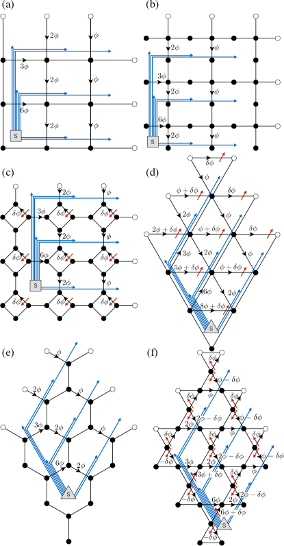
Figure 1: (Color online) Sketches of $3\times 3$ (a) square, (b) Lieb, (c) square-octagon, (d) triangular, (e) honeycomb and (f) kagome lattices with the string gauge under periodic boundary condition.

In Fig. 2(a), the energy gaps of the systems with $N\times N$ square and triangular lattices are plotted as functions of $\phi=N_{\phi}/N^{2}$. Since the energy scale is described by the Landau gap of the non-interacting case $E_{\text{LG}}$ and $\sum_{<i,j>}n_{i}n_{j}\sim\sum_{<i,j>}\rho^{2}\sim\rho$, the energy gap $\Delta\tilde{E}$ is scaled by $V\rho E_{\text{LG}}$. The results in Fig. 2(a) show that the scaling law $\Delta\tilde{E}\propto V\rho E_{\text{LG}}$ is valid in the wide range of $\phi$, regardless of the lattice types. Since the Landau gap $E_{\text{LG}}$ and $\rho=(N_{\text{e}}/\alpha N_{\phi})\phi$ are proportional to $\phi$, Fig. 2(a) indicates the relation $\Delta\tilde{E}\,\propto\phi^{2}\,\propto\rho^{2}$, which means that the excitations are local at both $\nu=1/3$ and $1/2$.

The difference between $\nu=1/3$ and $1/2$ becomes clear when we consider the dependence of energy gaps on the Landau degeneracy $N_{\phi}$. The numerically obtained $1/N_{\phi}$ dependence of the energy gaps is shown in Figs. 2(b) and (c), where we consider six types of lattice structures: square, Lieb, square-octagon, triangular, honeycomb, and kagome. The first three have square Bravais lattice while the last three have hexagonal Bravais lattice. Here, the systems with $\phi=1/N_{\phi}$ on the $N_{\phi}\times N_{\phi}$ lattices are considered. Note that the scaling found in Fig. 2(a) is independent of $\phi$. In Figs. 2(b) and (c), the energy gaps behave similarly as a function of $1/N_{\phi}$ if the underlying Bravais lattice is the same. In addition, Fig. 2(b) indicates the finite energy gap in the large $N_{\phi}$ limit, which is consistent with the Laughlin state as a ground state for $\nu=1/3$. On the other hand, for $\nu=1/2$, their $1/N_{\phi}$ dependence is clearly different from that for $\nu=1/3$ and can be consistent with the gap closing behavior.

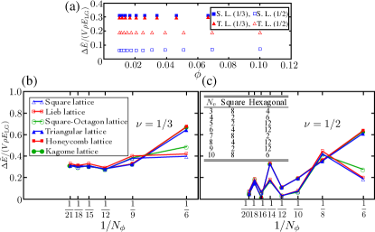
Figure 2: (Color online) Scaled energy gaps as functions of (a) the magnetic flux $\phi$ and (b,c) the inverse of Landau degeneracy $1/N_{\phi}$. The results are displayed for 5 electrons on square lattices (S.L.) and triangular lattices (T.L.) at $\nu=1/3$ and $1/2$ in (a). The table in (c) represents the degeneracies of the ground states at $\nu=1/2$ for the square Bravais lattice and the hexagonal one.

Another important quantity that characterizes the difference between the odd-denominator filling fractions (e.g. $\nu=1/3$) and the even-denominator ones (e.g. $\nu=1/2$) is the degeneracy of the ground state. The ground states for $\nu=1/3$ are always accompanied by the three-fold topological degeneracy [22]. This feature holds irrespective of the lattice type, which is explained by the translation of the center-of-mass.

In contrast, the degeneracy of the ground states at $\nu=1/2$ has no such universal feature. The ground state degeneracy for $\nu=1/2$ is shown in the inset table in Fig. 2(c). The degeneracy is always even, which is supported by the center-of-mass translation, and depends on the number of electrons and the underlying Bravais lattice. The many-electron system having interactions in a magnetic field with $\nu=1/2$ is mapped to the Fermi liquid with composite fermions [11, 23]. Without any magnetic field, there is a $Q$-fold rotational symmetry around the origin in the band structure, when the considered lattice type has the square Bravais lattice ($Q$=4) or the hexagonal one ($Q$=6). Thus, as long as $N_{1}=N_{2}$ and the system is not too small, the ground state of the many-electron state forms a close shell and the total momentum is zero, when the number of electrons is $1+Qn$, ($n$: integer). In fact, in the table in Fig. 2(c), the ground states have no degeneracy for $N_{\text{e}}=1+Qn$, if we ignore the factor of two given by the center-of-mass translational symmetry ($N_{\text{e}}=$5 and 9 for the square Bravais lattice and $N_{\text{e}}=7$ for the hexagonal one). Besides, the trend seen in Fig. 2(c) is that the energy gaps of the ground state forming a close shell are larger than those of the other states. These observations are consistent with the existence of the Fermi surface of the composite fermions.

As we have seen, the ground state at $\nu=1/3$ has a three-fold topological degeneracy. Then according to the Niu-Thouless-Wu formula [12], the Hall conductance is given by $\sigma_{xy}=\frac{e^{2}}{h}\frac{C}{m}$, where $C=\frac{1}{2\pi i}\int_{T^{2}}\hbox{Tr }{\bm{F}}$, ${\bm{F}}=d{\bm{A}}+{\bm{A}}^{2}$, and ${\bm{A}}$ is the non-Abelian Berry connection[24], which is given by the ground state multiplet $\Phi=(|G_{1}\rangle,\ldots,|G_{m}\rangle)$ as ${\bm{A}}=\Phi^{\dagger}d\Phi$ [25, 26]. Here, $|G_{i}\rangle$ are the ground states with $m$-fold topological degeneracy ($\langle G_{i}|G_{j}\rangle=\delta_{ij}$). The domain of integration $T^{2}$ is a parameter space given by the twisted boundary condition. We evaluate the Hall conductance by computing the Chern number explicitly using the ground state multiplet.

To obtain the Chern number, we impose a twisted boundary condition as $c^{\dagger}_{(n_{x}+N_{x},n_{y},s)}=e^{i\theta_{x}}c^{\dagger}_{(n_{x},n_{y},s)}$ and $c^{\dagger}_{(n_{x},n_{y}+N_{y},s)}=e^{i\theta_{y}}c^{\dagger}_{(n_{x},n_{y},s)}$, where $(n_{x},n_{y},s)$ is the site index ($n_{x}\in\{1,\cdots,N_{x}\}$, $n_{y}\in\{1,\cdots,N_{y}\}$, $s\in\{1,\cdots,\alpha\}$). The eigenvectors of the lowest LL $\psi_{k}$’s depend on $\theta=(\theta_{x},\theta_{y})$ through the dependence of $H_{\text{kin}}(\theta)$, which causes a modification on the projected interaction Hamiltonian as

$$\tilde{H}_{\text{int}}(\theta)=\sum_{k,l,m,n}V_{klmn}(\theta)d^{\dagger}_{k}(\theta)d^{\dagger}_{l}(\theta)d_{m}(\theta)d_{n}(\theta),$$ (2)

where $d^{\dagger}_{k}(\theta)=\bm{c}^{\dagger}\psi_{k}(\theta)$.

By diagonalizing $\tilde{H}_{\text{int}(\theta)}$, we obtain an $m$-component ground state multiplet as $\Phi(\theta)=(|G_{1}(\theta)\rangle,|G_{2}(\theta)\rangle,\ldots,|G_{m}(\theta)\rangle)$, where $|G_{i}(\theta)\rangle$’s are the $m$-fold degenerate ground states of $\tilde{H}_{\text{int}}$ satisfying $\langle G_{i}|G_{j}\rangle=\delta_{ij}$. By using this multiplet, the Chern number is evaluated by applying the method proposed in ref. doi:10.1143/JPSJ.74.1674. A $U(1)$ link variable on a discretized link in the parameter space is defined as $U_{\mu}(\theta_{l})=\frac{1}{N_{\mu}(\theta_{l})}\,\det[\Phi^{\dagger}(\theta_{l})\Phi(\theta_{l}+\Delta_{\mu})]$, where $\Delta_{\mu}$ represents the displacement in the direction $\mu=x,y$ at $\theta_{l}$ and $N_{\mu}(\theta_{l})=|\det[\Phi^{\dagger}(\theta_{l})\Phi(\theta_{l}+\Delta_{\mu})]|$. As seen from the definition, the link variables require the computation of the overlap between the ground states at $\theta_{l}$ and $\theta_{l}+\Delta_{\mu}$.

When $\tilde{H}_{\text{int}}(\theta)$ is diagonalized by the orthonormal basis $\Psi(\theta)=(|\Psi_{1}(\theta)\rangle,|\Psi_{2}(\theta)\rangle,\cdots,|\Psi_{N_{\text{D}}}(\theta)\rangle)$ ($N_{\text{D}}={}_{N_{\phi}}\!C_{N_{\text{e}}}$), the eigenvalue equation $\tilde{h}_{\text{int}}(\theta){\bm{u}}_{i}(\theta)=\tilde{E}_{i}(\theta){\bm{u}}_{i}(\theta)$, where $\tilde{h}_{\text{int}}=\Psi(\theta)^{\dagger}\tilde{H}_{\text{int}}(\theta)\Psi(\theta)$, is given and the ground state is expressed as

$$|G_{k}(\theta)\rangle=\Psi(\theta){\bm{u}}_{k}(\theta),$$ (3)

where $\tilde{E}_{k}(\theta)$ is one of the energies of the ground state multiplet. Using this expression, the overlap between the states with different boundary conditions, $\theta$ and $\theta^{\prime}$, is given by

$$\langle G_{k}(\theta)|G_{l}(\theta^{\prime})\rangle={\bm{u}}_{G_{k}}^{\dagger}(\theta)O(\theta,\theta^{\prime}){\bm{u}}_{G_{l}}(\theta^{\prime}),$$ (4)

$$O(\theta,\theta^{\prime})=\Psi^{\dagger}(\theta)\Psi(\theta^{\prime}).$$ (5)

The $(i,j)$ element of $O(\theta,\theta^{\prime})$ is expressed as $O_{ij}(\theta,\theta^{\prime})=\det[\tilde{\psi}_{i}(\theta)^{\dagger}\tilde{\psi}_{j}(\theta^{\prime})]$, where $\tilde{\psi_{i}}(\theta)=(\psi_{i_{1}}(\theta),\cdots,\psi_{i_{N_{\text{e}}}}(\theta))$. [28]

After obtaining the link variable in the above way, the lattice Berry curvature is defined as

$$\tilde{F}_{12}(\theta_{l})=\mathrm{Log}[U_{1}(\theta_{l})U_{2}(\theta_{l}+\Delta_{1})U_{1}^{-1}(\theta_{l}+\Delta_{2})U_{2}^{-1}(\theta_{l})]$$ (6)

and $-\pi<\tilde{F}_{12}(\theta_{l})/i\leq\pi$. The function $\mathrm{Log}$ means taking the principle branch of the logarithm. By definition, $\tilde{F}_{12}(\theta_{l})$ is invariant under the $U(m)$ gauge transformation $\Phi(\theta)\rightarrow\Phi^{\prime}(\theta)=\Phi(\theta)\omega(\theta)$. Now, the Chern number on the lattice is given as

$$\tilde{C}=\frac{1}{2\pi i}\sum_{l}\tilde{F}_{12}(\theta_{l}),$$ (7)

where the summation is taken over all the mesh points in the parameter space. It is guaranteed that $\tilde{C}$ is always integral and becomes exact in the limit of the fine mesh.

We diagonalize $\tilde{h}_{\text{int}}(\theta)$ for $\nu=1/3$ and its energy $\tilde{E}_{i}(\theta)$ is plotted as shown in Fig. 3(a). There is no level crossing between the ground state multiplet with the three-fold topological degeneracy and excited states.

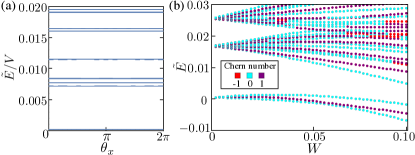
Figure 3: (Color online) (a)The eigenvalue of $\tilde{H}_{\text{int}}$ at $\nu=1/3$ against $\theta_{x}$ for $\theta_{y}=0$. The system with $12\times 12$ square lattices for $\phi=1/12$ is considered. The ground state is accompanied with the $3$-fold degeneracy in arbitrary parameters $\theta$ and well separated from the first excited states. (b)The eigenvalue of $\tilde{H}_{\text{int}}+\tilde{H}_{\text{imp}}$ at $\nu=1/3$ under the periodic boundary condition against the strength of random potential $W$. The system with $9\times 9$ square lattices for $\phi=1/9$ is considered and we set $V=1$. The Chern numbers are expressed by the color of plots.

For $\nu=1/3$, the Chern number of the ground state multiplet is 1. This means that the quantized Hall conductance is $e^{2}/3h$. On the other hand, the other excited states have $3n$-fold $(n:\text{integer})$ degeneracy and the Chern number is $n$, which indicates that the average of the Hall conductance is written as $\langle\sigma_{xy}\rangle=e^{2}/3h$ for any temperature. At $\nu=1/2$, as mentioned previously, the degeneracy of the ground states is generically $2n$ $(n:\text{integer})$. In this case, the Chern number of the ground state multiplet is $n$. In general, the Hall conductance specified by the Chern number of the ground state multiplet for the filling factor $\nu$ is evaluated as $\nu e^{2}/h$.

We also investigate the effects of disorder. We limit ourselves to the cases where the disorder potential is sufficiently small compared with the Landau gap, which allows us to discuss the impurity effects within the states projected to the lowest LL. We define the projected impurity potential as

$$\tilde{H}_{\text{imp}}=\sum_{i}w_{i}\tilde{c}^{\dagger}_{i}\tilde{c}_{i},$$ (8)

where $w_{i}=Wf_{i}$ is the site potential at a site $i$, $f_{i}$ represents uniform random numbers between $[-1/2,1/2]$, and $W$ is the strength of the random potential. In Fig. 3(b), the energy spectrum of $\tilde{H}_{\text{int}}+\tilde{H}_{\text{imp}}$ (for $\theta=0$) is plotted against $W$ with the Chern number indicated using different colors. In general, the topological degeneracy is lifted by the disorder in any value of $\theta$, and therefore, the Chern numbers can be individually assigned to each lifted state [29]. More specifically, the three-component ground state multiplet is split into three states, where one state carries a Chern number of 1, while the other two carry 0. This is topological stability. Furthermore, the numerical results suggest that the state with the lowest energy is always trivial in terms of the Chern number, which implies that the Hall conductance is zero when the temperature is smaller than the small energy gap within the lifted ground state multiplet.

To summarize, we construct the Peierls phase by using the string gauge for various types of lattices and analyze the many-electron states by using the Hamiltonian projected to the lowest LL. By diagonalizing the pseudopotential, a simple scaling form of the energy gap is obtained. The results for $\nu=1/3$ indicate that the ground states accompanied by three-fold topological degeneracy are consistent with the Laughlin state. On the other hand, the degeneracy of the ground state for $\nu=1/2$ depends on the type of lattice structure, which is discussed in terms of the composite fermion picture using the existence of the Fermi surface. We further formulate a method to compute the Chern number of the ground state multiplet using the pseudopotential. This method is applied to the lattice analogue of the Laughlin state and the effects of disorder are discussed with the Chern number. This work is partly supported by Grants-in-Aid for Scientific Research, (KAKENHI), Grant numbers 17H06138, 16K13845 and 25107005.

References

- [1] K. v. Klitzing, G. Dorda, and M. Pepper: Phys. Rev. Lett. 45 (1980) 494.
- [2] D. J. Thouless, M. Kohmoto, M. P. Nightingale, and M. den Nijs: Phys. Rev. Lett. 49 (1982) 405.
- [3] A. P. Schnyder, S. Ryu, A. Furusaki, and A. W. W. Ludwig: Phys. Rev. B 78 (2008) 195125.
- [4] X.-L. Qi, T. L. Hughes, and S.-C. Zhang: Phys. Rev. B 78 (2008) 195424.
- [5] A. Kitaev: AIP Conference Proceedings 1134 (2009) 22.
- [6] S. Ryu, A. P. Schnyder, A. Furusaki, and A. W. W. Ludwig: New Journal of Physics 12 (2010) 065010.
- [7] C. L. Kane and E. J. Mele: Phys. Rev. Lett. 95 (2005) 226801.
- [8] D. C. Tsui, H. L. Stormer, and A. C. Gossard: Phys. Rev. Lett. 48 (1982) 1559.
- [9] R. B. Laughlin: Phys. Rev. Lett. 50 (1983) 1395.
- [10] The Quantum Hall Effect, ed. R. E. Prange and S. M. Girvin (Springer-Verlag New York, 1990) 2nd ed.
- [11] J. K. Jain: Phys. Rev. Lett. 63 (1989) 199.
- [12] Q. Niu, D. J. Thouless, and Y.-S. Wu: Phys. Rev. B 31 (1985) 3372.
- [13] G. Möller and N. R. Cooper: Phys. Rev. Lett. 103 (2009) 105303.
- [14] A. Sterdyniak, N. Regnault, and G. Möller: Phys. Rev. B 86 (2012) 165314.
- [15] T. Neupert, L. Santos, C. Chamon, and C. Mudry: Phys. Rev. Lett. 106 (2011) 236804.
- [16] D. N. Sheng, Z.-C. Gu, K. Sun, and L. Sheng: Nature Communications 2 (2011) 389 EP .
- [17] N. Regnault and B. A. Bernevig: Phys. Rev. X 1 (2011) 021014.
- [18] Y.-L. Wu, B. A. Bernevig, and N. Regnault: Phys. Rev. B 85 (2012) 075116.
- [19] Y. Hatsugai, K. Ishibashi, and Y. Morita: Phys. Rev. Lett. 83 (1999) 2246.
- [20] Y. Hamamoto, H. Aoki, and Y. Hatsugai: Phys. Rev. B 86 (2012) 205424.
- [21] Y. Hatsugai, T. Morimoto, T. Kawarabayashi, Y. Hamamoto, and H. Aoki: New Journal of Physics 15 (2013) 035023.
- [22] F. D. M. Haldane: Phys. Rev. Lett. 55 (1985) 2095.
- [23] B. I. Halperin, P. A. Lee, and N. Read: Phys. Rev. B 47 (1993) 7312.
- [24] M. V. Berry: Proceedings of the Royal Society of London. A. Mathematical and Physical Sciences 392 (1984) 45.
- [25] Y. Hatsugai: Journal of the Physical Society of Japan 73 (2004) 2604.
- [26] Y. Hatsugai: Journal of the Physical Society of Japan 74 (2005) 1374.
- [27] T. Fukui, Y. Hatsugai, and H. Suzuki: Journal of the Physical Society of Japan 74 (2005) 1674.
- [28] , where .
- [29] D. J. Thouless: Phys. Rev. B 40 (1989) 12034.