Proton decay testing low energy SUSY

Abstract

We show that gauge coupling unification in SUSY models can make a non-trivial interconnection between collider and proton decay experiments. Under the assumption of precise gauge coupling unification in the MSSM, the low energy SUSY spectrum and the unification scale are intertwined, and the lower bound on the proton lifetime can be translated into upper bounds on SUSY masses. We found that the current limit on $\tau(p\to\pi^{0}　e^{+})$ already excludes gluinos and winos $heavier$ than $\sim 120$ and 40 TeV, respectively, if their mass ratio is $M_{3}/M_{2}\sim 3$. Next generation nucleon decay experiments are expected to bring these upper bounds down to $\sim 10$ and 3 TeV.

Proton decay would be the key evidence for grand unified theories (GUTs) Langacker:1980js . Among possible decay channels, a special role is played by the $p\rightarrow\pi^{0}e^{+}$ mode for which the dominant contribution may come from the $D=6$ operators depending almost exclusively on the $X,Y$ boson mass and the unified gauge coupling. This is in contrast to the other channels induced by $D=5$ operators, which depend on many more parameters, though the rate is typically larger than the $p\rightarrow\pi^{0}e^{+}$ mode.

The main point we want to emphasise and make very explicit in this Letter is that $\tau_{p\rightarrow\pi^{0}e^{+}}$ carries an important information about the low scale supersymmetric (SUSY) spectrum. To this end we assume here that the unification of the gauge couplings is precise (or exact) within the minimal SUSY Standard Model (MSSM) without threshold corrections of GUT scale particles Raby:2009sf . In fact, there exists a class of models where these corrections are absent or highly suppressed (see e.g. Kawamura:2000ev ). On the other hand, GUT threshold corrections in conventional models are often too large compared to the typical mismatch of gauge couplings at a high scale in the MSSM (see Ellis:2015jwa for a recent discussion). This means that the well-known “success of gauge coupling unification in the MSSM”, if not a mere accident, may favour the aforementioned class of models as the correct theory of grand unification.

Under the assumption of precise gauge coupling unification (GCU) in the MSSM, we show that the low energy SUSY spectrum and the unification scale are intertwined, and the lower bound on the proton lifetime $\tau_{p\rightarrow\pi^{0}e^{+}}$ can be translated into upper bounds on SUSY masses. This leads to an interesting interconnection between the proton decay experiments and the collider searches, particularly in view of the future progress on both fronts, in cornering supersymmetric spectrum from above and from below.

At the one-loop the gauge couplings at scale $\tilde{\mu}$ in the MSSM is given by

$$\frac{2\pi}{\alpha_{i}(\tilde{\mu})}\,=\,\frac{2\pi}{\alpha_{i}(m_{Z})}-b_{i}\,\ln\Big{(}\frac{\tilde{\mu}}{m_{Z}}\Big{)}+s_{i}.$$ (1)

where $\alpha_{1}\equiv\frac{3}{5}\alpha_{Y}$, $i=1,2,3$ represents the gauge group, $b_{i}=(\frac{33}{5},1,-3)$ are the one-loop $\beta$-function coefficients for the MSSM and

$$s_{i}\,\equiv\,\sum_{\eta}b_{i}^{\eta}\ln\Big{(}\frac{m_{\eta}}{m_{Z}}\Big{)}$$ (2)

are the threshold corrections of SUSY particles. For SUSY particle $\eta$, the mass and its contribution to $b_{i}$ are given by $m_{\eta}$ and $b_{i}^{\eta}$, respectively.

In the special case where all SUSY particles are mass degenerate at $M_{s}$, the threshold correction can be written as $s_{i}=\delta_{i}\ln(M_{s}/m_{Z})$ with $\delta_{i}\equiv(b_{i}-b_{i}^{\rm SM})$, where $b_{i}^{\rm SM}=(\frac{41}{10},-\frac{19}{6},-7)$ are the one-loop $\beta$-function coefficients for the Standard Model (SM). In this case, exact gauge unification $\alpha_{1}(\tilde{\mu})=\alpha_{2}(\tilde{\mu})=\alpha_{3}(\tilde{\mu})\equiv\alpha_{G}^{*}$ is achieved by the particular values of $M_{s}$ and $\tilde{\mu}$: $M_{s}^{*}$, $M_{G}^{\rm deg*}$, satisfying

$$\frac{2\pi}{\alpha_{G}^{*}}-\frac{2\pi}{\alpha_{i}(m_{Z})}+b_{i}\,\ln\Big{(}\frac{M^{\rm deg*}_{G}}{m_{Z}}\Big{)}\,=\,\delta_{i}\,\ln\Big{(}\frac{M_{s}^{*}}{m_{Z}}\Big{)}$$ (3)

for all $i$. It should be kept in mind that the quantities $M_{s}^{*}$, $M_{G}^{\rm deg*}$ and $\alpha_{G}^{*}$ are not variables but constants defined as the solution to the above three simultaneous equations.

Coming back to the general case, let us decompose the vector $s_{i}$ into three independent vectors as Krippendorf:2013dqa

$$s_{i}\,=\,\delta_{i}\,\ln\Big{(}\frac{T}{m_{Z}}\Big{)}+b_{i}\ln\Omega+C\,.$$ (4)

The solution to this set of equations is given by

$$\ln\Big{(}\frac{T}{m_{Z}}\Big{)} = v_{i}s_{i}/D$$ (5)

$$\ln\Omega = u_{i}s_{i}/D$$ (6)

$$C = \epsilon_{ijk}\delta_{j}b_{i}s_{k}/D$$ (7)

where summation is understood for the repeated indices and $\epsilon_{ijk}$ is the antisymmetric tensor and

$$v\,=\,\begin{pmatrix}b_{2}-b_{3}\\ -b_{1}+b_{3}\\ b_{1}-b_{2}\end{pmatrix},~{}~{}~{}u\,=\,\begin{pmatrix}-\delta_{2}+\delta_{3}\\ \delta_{1}-\delta_{3}\\ -\delta_{1}+\delta_{2}\end{pmatrix},$$

$$D~{}=~{}b_{2}\delta_{1}-b_{3}\delta_{1}-b_{1}\delta_{2}+b_{3}\delta_{2}+b_{1}\delta_{3}-b_{2}\delta_{3}\,.$$ (8)

Plugging the concrete values of $b_{i}$, $\delta_{i}$ and $b_{i}^{\eta}$ into these expressions, one gets

$$T = \Big{[}M_{3}^{-28}M_{2}^{32}(\mu^{4}m_{A})^{3}X_{T}\Big{]}^{\frac{1}{19}},$$ (9)

$$\Omega = \Big{[}M_{3}^{-100}M_{2}^{60}(\mu^{4}m_{A})^{8}X_{\Omega}\Big{]}^{\frac{1}{288}}\,,$$ (10)

$$C = \frac{125}{19}\ln M_{3}-\frac{113}{19}\ln M_{2}-\frac{40}{19}\ln\mu-\frac{10}{19}\ln m_{A}$$ (11)

$$+ \sum_{i=1...3}\Big{[}\frac{79}{114}\ln m_{\tilde{d}_{Ri}}-\frac{10}{19}\ln m_{\tilde{l}_{i}}-\frac{121}{114}\ln m_{\tilde{q}_{i}}$$

$$+ \frac{257}{228}\ln m_{\tilde{u}_{Ri}}+\frac{33}{76}\ln m_{\tilde{e}_{Ri}}\Big{]}\,.$$

with

$$X_{T} \equiv \prod_{i=1...3}\Big{(}\frac{m^{3}_{\tilde{l}_{i}}}{m^{3}_{\tilde{d}_{Ri}}}\Big{)}\Big{(}\frac{m^{7}_{\tilde{q}_{i}}}{m^{2}_{\tilde{e}_{Ri}}m^{5}_{\tilde{u}_{Ri}}}\Big{)}\,,$$ (12)

$$X_{\Omega} \equiv \prod_{i=1...3}\Big{(}\frac{m^{8}_{\tilde{l}_{i}}}{m^{8}_{\tilde{d}_{Ri}}}\Big{)}\Big{(}\frac{m^{6}_{\tilde{q}_{i}}m_{\tilde{e}_{Ri}}}{m^{7}_{\tilde{u}_{Ri}}}\Big{)}\,.$$ (13)

The SUSY mass parameters appearing in this Letter should be understood as the magnitude of the corresponding parameters because phase factors do not affect RG running. In most models, the sfermion contributions to $T$ and $\Omega$ are negligible (i.e. $X_{T}\sim X_{\Omega}\sim 1$). In particular, these contributions vanish if the masses are degenerate within the SU(5) multiplets, ${\bf\bar{5}}_{i}=(\tilde{d}_{R}^{c},\tilde{l})_{i}$, ${\bf 10}_{i}=(\tilde{q},\tilde{u}_{R}^{c},\tilde{e}_{R}^{c})_{i}$. One can explicitly check that for a degenerate spectrum, $\ln\Omega=C=0$.

To see roles of $T$, $\Omega$ and $C$ in gauge unification, we substitute Eq. (4) into Eq. (1) and obtain

$$\frac{2\pi}{\alpha_{i}(\tilde{\mu})}=\frac{2\pi}{\alpha_{G}^{*}}-b_{i}\ln\Big{(}\frac{\tilde{\mu}}{\Omega M^{\rm deg*}_{G}}\Big{)}+\delta_{i}\ln\Big{(}\frac{T}{M_{s}^{*}}\Big{)}+C,$$ (14)

where Eq. (3) has also been used. It is clear that the exact unification for the general case is obtained when the right-hand-side (RHS) becomes $i$-independent, that is at $T=M_{s}^{*}$ Carena:1993ag and the exact unification scale is given by

$$M_{G}\,=\,\Omega M^{\rm deg*}_{G}\,.$$ (15)

The unified gauge coupling is related to that of the degenerate case as

$$\alpha^{-1}_{G}\,=\,\alpha^{*-1}_{G}+\,\frac{C}{2\pi}.$$ (16)

Away from the exact unification, we define a candidate unification scale $M_{U}$ and a semi-unified coupling $\alpha_{U}$ by $\alpha_{1}(M_{U})=\alpha_{2}(M_{U})\equiv\alpha_{U}$. This scale can be computed from a low energy spectrum as $M_{U}=\Omega M^{\rm deg*}_{G}(T/M_{s}^{*})^{\frac{\delta_{1}-\delta_{2}}{b_{1}-b_{2}}}$, and at this scale the gauge couplings are given by

$$\frac{2\pi}{\alpha_{i}(M_{U})}\,=\,\frac{2\pi}{\alpha_{G}^{*}}\,+\Big{(}\delta_{i}-b_{i}\frac{\delta_{1}-\delta_{2}}{b_{1}-b_{2}}\Big{)}\ln\Big{(}\frac{T}{M_{s}^{*}}\Big{)}+\,C\,.$$ (17)

Using this formula, a measure of gauge coupling unification, which we define as $\epsilon_{3}\equiv(\alpha_{3}(M_{U})-\alpha_{U})/\alpha_{U}$, is calculated as

$$\epsilon_{3}\,=\,\frac{\alpha_{G}^{*}}{2\pi}\,Y\,\ln\Big{(}T/M_{s}^{*}\Big{)}\,+\,\cdots,$$ (18)

where the dots represent higher order terms of $\frac{\alpha_{G}^{*}}{2\pi}$ and

$$Y~{}\equiv~{}\frac{b_{1}(\delta_{2}-\delta_{3})+b_{2}(-\delta_{1}+\delta_{3})+b_{3}(\delta_{1}-\delta_{2})}{b_{1}-b_{2}}\,.$$ (19)

It is interesting that $\epsilon_{3}$ depends only on $T$ at the leading order Carena:1993ag .

Our argument so far is based on the one-loop renormalization group equations (RGEs). It turns out that the relations Eqs. (15), (16) and (18) still hold numerically with a good accuracy at two-loop level if the constants are replaced by the two-loop corrected values: $M_{s}^{*}=2.08$ TeV, $M_{U}^{\rm deg*}=1.27\cdot 10^{16}$ GeV and $\alpha_{G}^{*-1}=25.5$.

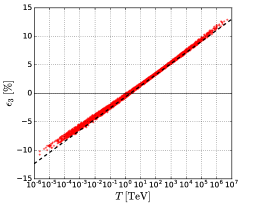
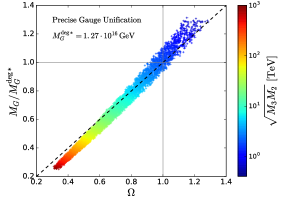
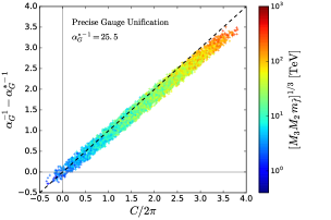
Figure 1: A scan of SUSY particle masses projected onto the ($T$, $\epsilon_{3}$) (top), the ($\Omega$, $M_{G}/M_{G}^{\rm deg*}$) (middle) and ($C/2\pi$, $\alpha_{G}^{-1}-\alpha_{G}^{*-1}$) (bottom) planes. In the middle and bottom plots, the precise gauge unification $(|\epsilon_{3}|<0.1\%)$ is required, and the colour-codes represent typical SUSY scales $\sqrt{M_{3}M_{2}}$ and $(M_{3}M_{2}m_{\tilde{f}})^{\frac{1}{3}}$, respectively. The dashed lines represent the one-loop relations Eq. (18), (15) and (16) for the top, middle and bottom plots, respectively.

We show in Fig. 1 the result of our numerical scan. All numerical scans presented in this Letter use a two-loop RGE code including the effect of the top Yukawa coupling, following Langacker:1992rq . We use $\tan\beta=10$ but a variation of $\tan\beta$ results in negligible effects. The SUSY breaking parameters are uniformly scanned in the logarithmic scale within [$m_{\min}$, $10^{3}$ TeV]. We take $m_{\rm min}=1.5$ TeV for $M_{3}$ and 200 GeV for $M_{2},\mu$ and $m_{A}$. The sfermion masses are assumed to be universal ($\equiv m_{\tilde{f}}$) for simplicity and $m_{\min}=1$ TeV is used. We also vary $\alpha_{3}(m_{Z})=0.1184(7)$, according to the 1-$\sigma$ uncertainty.

The top plot in Fig. 1 tests the predicted relation Eq. (18) (dashed line). We see that the exact unification occurs only when the SUSY masses are arranged such that $T$ computed by Eq. (9) is within a certain range [1, 4] TeV centred around $\sim 2$ TeV. The width of $T$ for exact unification comes mainly from the uncertainty on $M_{s}^{*}$ due to the variation of $\alpha_{3}(m_{Z})$. The middle plot shows the correlation between $\Omega$ and the exact unification scale, $M_{G}$. Hereafter, we require a precise gauge unification, $|\epsilon_{3}|<0.1\%$. The dashed line corresponds to Eq. (15). The colour of points represents a typical SUSY scale $\sqrt{M_{3}M_{2}}$. One can see that heavy SUSY tends to have a small unification scale. For the PeV scale SUSY with $\sqrt{M_{3}M_{2}}\sim 10^{3}$ TeV, $M_{G}$ is reduced by a factor of 5 compared to the TeV scale one. The bottom plot confirms the predicted relation Eq. (16) (dashed line). The colour-code indicates a SUSY scale, $(M_{3}M_{2}\,m_{\tilde{f}})^{\frac{1}{3}}$. We see that high scale SUSY tends to predict a smaller unified coupling, $\alpha_{G}$, but the variation is small and only up to $\sim 10\%$ between the TeV and PeV scale SUSY mass points.

An interesting observation follows from the last two plots of Fig. 1. High scale SUSY, where the unification scale is lower, in general leads to a rapid proton decay, $p\to e^{+}\pi^{0}$. This is because the rate $\Gamma(p\to e^{+}\pi^{0})$ scales as $\alpha_{G}/(M_{G})^{4}$, where the $X,Y$ boson mass is identified as the unification scale, since the precise gauge unification implies all GUT particles charged under the SM gauge group have the same mass, $M_{G}$. Turning this around, the lower limit on $M_{G}$ from the proton lifetime measurement (if found, bearing in mind that the variation of $\alpha_{G}$ is small) can place upper bounds on the masses of SUSY particles. Let us denote this lower limit by $M_{PD}$: $M_{G}>M_{PD}$. Then, eliminating $M_{3}$ from Eq. (10) by using Eq. (9), Eq. (15) gives us

$$M_{2}^{\frac{4}{5}}(\mu^{4}m_{A})^{\frac{1}{25}}\,<\,M_{s}^{*}\cdot\Big{(}\frac{M^{\rm deg*}_{G}}{M_{PD}}\Big{)}^{\frac{2016}{475}}\cdot X_{\rm EW}^{\frac{1}{25}}\,,$$ (20)

where

$$X_{\rm EW}~{}\equiv\,\prod_{i=1...3}\Big{(}\frac{m_{\tilde{l}_{i}}}{m_{\tilde{d}_{Ri}}}\Big{)}\Big{(}\frac{m^{7}_{\tilde{q}_{i}}}{m^{3}_{\tilde{e}_{Ri}}m^{4}_{\tilde{u}_{Ri}}}\Big{)}\,.$$ (21)

This implies that the smallest mass in the LHS is bounded from above by the RHS of Eq. (20). When this bound is saturated, $M_{2}=\mu=m_{A}$. The upper limit on the individual parameters are obtained, for example, as

$$M_{2}\,<\,M_{s}^{*}\cdot\Big{(}\,\frac{M_{s}^{*5}}{\mu^{4}m_{A}}\,\Big{)}^{\frac{1}{20}}\cdot\Big{(}\frac{M_{G}^{\rm deg*}}{M_{PD}}\Big{)}^{\frac{504}{95}}\cdot X_{\rm EW}^{\frac{1}{20}}\,.$$ (22)

In this expression the RHS is bounded from above by the experimental lower limit on $\mu$ and $m_{A}$.

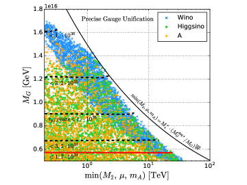
Figure 2: Points with precise gauge unification projected onto the ${\rm min}(M_{2},\mu,m_{A})$ vs $M_{G}$ plane. The blue, green and orange points correspond to the points where $M_{2}$, $\mu$ and $m_{A}$ is the smallest among them, respectively. The regions below a black-dashed or a red-solid line are excluded by the quoted future or current limits on the proton lifetime. The black-solid line represents the upper bound found at the one-loop level in Eq. (20).

The upper bound Eq. (20) is observed in our numerical scan shown in Fig. 2, where the smallest of $M_{2}$, $\mu$ and $m_{A}$ is plotted in the $x$-axis. The blue, green and orange points correspond to the cases where $M_{2}$, $\mu$ and $m_{A}$ is the lightest among the three, respectively. A tendency is observed that $M_{2}$ is close to the upper limit if $M_{2}$ is the lightest. This is due to the higher power for $M_{2}$ in Eq. (20) than for $\mu$ and $m_{A}$. At each point we calculate $\tau_{p\to\pi^{0}e^{+}}$ based on Babu:2013jba ; Bajc:2016qcc using $\alpha_{G}$ and $M_{G}$ obtained by the two-loop RGE code. The horizontal black-dashed and red-solid lines represent the boundaries where all points below them have the lifetime shorter than the quoted values. In particular, the region below the red line is excluded by the current limit: $\tau_{p\to\pi^{0}e^{+}}>1.7\cdot 10^{34}$ years Takhistov:2016eqm .

The upper bound on the gluino mass can be found by eliminating $\mu^{4}m_{A}$ in Eq. (10) by using Eq. (9) as

$$M_{3}\,<\,M_{s}^{*}\cdot\frac{M_{s}^{*}}{M_{2}}\cdot\Big{(}\frac{M_{G}^{\rm deg*}}{M_{PD}}\Big{)}^{\frac{216}{19}}\cdot X_{\tilde{g}}^{\frac{1}{4}}$$ (23)

with

$$X_{\tilde{g}}~{}\equiv\,\prod_{i=1...3}\Big{(}\frac{m_{\tilde{u}_{Ri}}m_{\tilde{e}_{Ri}}}{m^{2}_{\tilde{q}_{i}}}\Big{)}\,.$$ (24)

As previously, the RHS of Eq. (23) is bounded from above by the experimental lower limit on the wino mass.

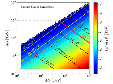
Figure 3: Points with precise gauge unification projected onto the ($M_{3}$, $M_{2}$) plane. The colour-code shows $(\mu^{4}m_{A})^{\frac{1}{5}}$. The regions above the black-dashed and red-solid lines are excluded by the quoted future or current limits on $\tau_{p\to\pi^{0}e^{+}}$. The three diagonal lines correspond to $R\equiv M_{3}/M_{2}=1$, 3 and 7 from top to bottom. In this plot the upper boundaries of $\mu$ and $m_{A}$ scans are extended up to $10^{7}$ TeV.

If the SUSY breaking mechanism is specified, the ratio of gluino and wino masses is usually predicted. Assuming the value of $R\equiv M_{3}/M_{2}$, the following upper bounds can be derived:

$$M_{3} < M_{s}^{*}\cdot R^{\frac{1}{2}}\cdot\Big{(}\frac{M_{G}^{\rm deg*}}{M_{PD}}\Big{)}^{\frac{108}{19}}\cdot X_{\tilde{g}}^{\frac{1}{8}}\,,$$ (25)

$$(\mu^{4}m_{A})^{\frac{1}{5}} < M_{s}^{*}\cdot R^{2}\cdot\Big{(}\frac{M_{PD}}{M^{\rm deg*}_{G}}\Big{)}^{\frac{144}{90}}\cdot X_{\mu}^{\frac{1}{10}}\,,$$ (26)

where

$$X_{\mu}~{}\equiv\,\prod_{i=1...3}\Big{(}\frac{m^{2}_{\tilde{l}_{i}}}{m^{2}_{\tilde{d}_{Ri}}}\Big{)}\Big{(}\frac{m^{4}_{\tilde{q}_{i}}}{m_{\tilde{e}_{Ri}}m^{3}_{\tilde{u}_{Ri}}}\Big{)}\,.$$ (27)

We show in Fig. 3 our scan in the $(M_{3},M_{2})$ plane with the colour-code indicating $(\mu^{4}m_{A})^{\frac{1}{5}}$. As previously, the black-dashed and red-solid lines represent the future and current bounds on $\tau_{p\to\pi^{0}e^{+}}$. It is evident that $M_{3}$ and $M_{2}$ are highly sensitive to the proton lifetime and constrained by it from above. This is in direct contrast to collider searches, constraining these parameters from below. Unlike $M_{3}$ and $M_{2}$, $\mu$ and $m_{A}$ are almost insensitive to the proton lifetime, which follows from the lower power of $M_{PD}$ in Eq. (26). On the other hand, they are highly sensitive to $R$. In particular, $\mu$ is typically a TeV for $R=1$ whereas it is ${\cal O}(100)$ TeV for $R=7$. The implication of this to naturalness and phenomenology are studied in detail in Raby:2009sf ; Krippendorf:2013dqa ; us .

It is remarkable that the current proton lifetime limit already excludes the gluino and wino masses larger than 200 and 30 TeV for $R\sim 7$ (e.g. AMSB) and 120 and 40 TeV for $R\sim 3$ (e.g. CMSSM, GMSB), respectively. Next generation nucleon decay experiments are expected to improve the current $\tau_{p\to\pi^{0}e^{+}}$ limit by a factor of ten Babu:2013jba , which will result in tightening the upper bounds on gluino and wino masses further down to $(M_{3},M_{2})\lesssim(10,\,3)$ TeV for $R\sim 3$ and $(M_{3},M_{2})\lesssim(15,\,2)$ TeV for $R\sim 7$. These bounds are close to the lower mass limits $(M_{3},M_{2})\gtrsim(10,\,2.7)$ TeV Cohen:2013xda ; Low:2014cba , which are expected to be obtained at future 100 TeV hadron-hadron colliders.

We have investigated the link between the proton lifetime $\tau_{p\to\pi^{0}e^{+}}$ and the supersymmetric spectrum under the assumption of vanishing GUT thresholds. It has been shown that most of the allowed mass range of gluinos and winos will be probed by future collider and proton lifetime experiments. It will also be interesting to extend this study to models with non-vanishing GUT threshold corrections (see e.g. Hisano:2013cqa ).

References

(1)
For early references see, P. Langacker,
Phys. Rept. 72 (1981) 185.
(2)
S. Raby, M. Ratz and K. Schmidt-Hoberg,
Phys. Lett. B 687 (2010) 342
[arXiv:0911.4249 [hep-ph]].
(3)
Y. Kawamura,
Prog. Theor. Phys. 105 (2001) 999
[hep-ph/0012125];
L. J. Hall and Y. Nomura,
Phys. Rev. D 64 (2001) 055003
[hep-ph/0103125];
A. Hebecker and M. Trapletti,
Nucl. Phys. B 713 (2005) 173
[hep-th/0411131].
(4)
S. A. R. Ellis and J. D. Wells,
Phys. Rev. D 91 (2015) no.7, 075016
[arXiv:1502.01362 [hep-ph]];
S. A. R. Ellis and J. D. Wells,
arXiv:1706.00013 [hep-ph].
(5)
G. F. Giudice and A. Strumia,
Nucl. Phys. B 858 (2012) 63
[arXiv:1108.6077 [hep-ph]];
M. Ibe and T. T. Yanagida,
Phys. Lett. B 709 (2012) 374
[arXiv:1112.2462 [hep-ph]];
E. Bagnaschi, G. F. Giudice, P. Slavich and A. Strumia,
JHEP 1409 (2014) 092
[arXiv:1407.4081 [hep-ph]].
(6)
N. Arkani-Hamed, A. Delgado and G. F. Giudice,
Nucl. Phys. B 741 (2006) 108
[hep-ph/0601041];
J. Hisano, S. Matsumoto, M. Nagai, O. Saito and M. Senami,
Phys. Lett. B 646 (2007) 34
[hep-ph/0610249];
J. Ellis, F. Luo and K. A. Olive,
JHEP 1509 (2015) 127
[arXiv:1503.07142 [hep-ph]].
(7)
S. Krippendorf, H. P. Nilles, M. Ratz and M. W. Winkler,
Phys. Rev. D 88 (2013) 035022
[arXiv:1306.0574 [hep-ph]].
(8)
M. Carena, S. Pokorski and C. E. M. Wagner,
Nucl. Phys. B 406 (1993) 59
[hep-ph/9303202].
(9)
P. Langacker and N. Polonsky,
Phys. Rev. D 47 (1993) 4028
[hep-ph/9210235].
(10)
K. S. Babu et al.,
arXiv:1311.5285 [hep-ph].
(11)
B. Bajc, J. Hisano, T. Kuwahara and Y. Omura,
Nucl. Phys. B 910 (2016) 1
[arXiv:1603.03568 [hep-ph]].
(12)
H. Murayama and A. Pierce,
Phys. Rev. D 65 (2002) 055009
[hep-ph/0108104].
(13)
V. Takhistov [Super-Kamiokande Collaboration],
arXiv:1605.03235 [hep-ex].
(14)
S. Pokorski, K. Rolbiecki, K.Sakurai,
in preparation.
(15)
T. Cohen, T. Golling, M. Hance, A. Henrichs, K. Howe, J. Loyal, S. Padhi and J. G. Wacker,
JHEP 1404 (2014) 117
[arXiv:1311.6480 [hep-ph]].
(16)
M. Low and L. T. Wang,
JHEP 1408 (2014) 161
[arXiv:1404.0682 [hep-ph]].
(17)
J. Hisano, T. Kuwahara and N. Nagata,
Phys. Lett. B 723 (2013) 324
[arXiv:1304.0343 [hep-ph]].