SN 1986J VLBI. IV. The Nature of the Central Component

Abstract

We report on VLA measurements between 1 and 45 GHz of the evolving radio spectral energy distribution (SED) of SN 1986J, made in conjunction with VLBI imaging. The SED of SN 1986J is unique among supernovae, and shows an inversion point and a high-frequency turnover. Both are due to the central component seen in the VLBI images, and both are progressing downward in frequency with time. The optically-thin spectral index of the central component is almost the same as that of the shell. We fit a simple model to the evolving SED consisting of an optically-thin shell and a partly-absorbed central component. The evolution of the SED is consistent with that of a homologously expanding system. Both components are fading, but the shell more rapidly. We conclude that the central component is physically inside the expanding shell, and not a surface hot-spot central only in projection. Our observations are consistent with the central component being due to interaction of the shock with the dense and highly-structured circumstellar medium that resulted from a period of common-envelope evolution of the progenitor. However a young pulsar-wind nebula or emission from an accreting black hole can also not be ruled out at this point.

1 Introduction

SN 1986J was one of the most radio luminous supernovae ever observed, and one of the few supernovae still detectable more than $t=30$ years after the explosion, thus we have been able to follow its evolution for longer than was possible for most other SNe. Its radio brightness and relatively close distance allowed both resolved very long baseline interferometry (VLBI) images and accurate estimations of its broadband radio spectral energy distribution (SED) to be made. This paper is the fourth in our series of papers on SN 1986J, Bietenholz et al. (2002, 2010) and Bietenholz & Bartel (2017b), which we will refer to as Papers I to III respectively. In this fourth paper in the series, we discuss mainly the evolution of the broadband radio SED, but with reference to the morphology as seen in the VLBI images.

For the convenience of the reader, we repeat some of the introductory material from Paper III here. SN 1986J was first discovered in the radio, some time after the explosion (van Gorkom et al., 1986; Rupen et al., 1987). The best estimate of the explosion epoch is $1983.2\pm 1.1$ ($t=0$, Paper I; see also Rupen et al., 1987; Chevalier, 1987; Weiler et al., 1990). It occurred in the nearby galaxy NGC 891, for whose distance the NASA/IPAC Extragalactic Database (NED) lists 19 measurements with a mean of $10.0\pm 1.4$ Mpc, which value we adopt throughout this paper.

Optical spectra, taken soon after the discovery, showed a somewhat unusual spectrum with narrow linewidths, but the prominent H$\alpha$ lines led to a classification as a Type IIn supernova (Rupen et al., 1987). It is an unusually long-lasting SN at all wavelengths, and has been detected in the optical (Milisavljevic et al., 2008), infrared (Tinyanont et al., 2016) and X-ray (Houck, 2005) more than two decades after the explosion. It has been observed with VLBI since 1987, and we refer the interested reader to a sequence of VLBI images in Paper III which show both the expansion and the non-selfsimilar evolution over almost three decades.

The structure seen in the VLBI images shows an expanding, albeit somewhat distorted shell, but also two strong compact enhancements of the brightness: one to the NE of the shell center, and a second at or very near the projected center. Such a central radio component has not so far been seen in any other supernova (see e.g., Bietenholz, 2014; Bartel & Bietenholz, 2014), making SN 1986J a particularly interesting case.

Figure 1: The 5-GHz VLBI image of SN 1986J made from observations on 2014 Oct. 23, at age 31.6 yr, reproduced from Paper III. The contours are drawn at $-3$, 3, 5, 10, 15, 20, 30, 50, 70 and 90% of the peak brightness, with the 50% contour being emphasized. The peak brightness was 617 $\mu$Jy beam^-1, the total CLEANed flux density was 1622 $\mu$Jy, and the background rms brightness was 5.9 $\mu$Jy beam^-1. The color-scale is labeled in $\mu$Jy beam^-1, and is saturated so as to better show the low-level emission. North is up and east to the left, and the FWHM of the convolving beam of 2.21 mas $\times\;0.89$ mas at p.a. $-15$° is indicated at upper left.

The radio emission from a supernova is synchrotron emission, and therefore the broadband SED reflects the underlying distributions of relativistic particles and free-free absorbing thermal matter, and holds important clues to the physics. The evolution of SN 1986J’s SED was quite unusual, as we discussed in Paper II. Usually, the SED of a SN evolves in a fairly predictable way: the flux density, $S_{\nu}$, at frequency, $\nu$, shows an optically thick rise at low frequencies up to a turnover frequency, and an optically-thin powerlaw above the turnover frequency, with values of the spectral index, $\alpha$, ($S_{\nu}\propto\nu^{\alpha}$) usually in the range of $-0.5$ to $-0.8$. The turnover frequency evolves downward in time, typically reaching 10 GHz at $t\sim 100$ d (see, e.g., Weiler et al., 2002). There is, however, a large variation in this timescale: for SN 1987A, for example, the turnover frequency reached 10 GHz at $t<1$ d (Turtle et al., 1987) while for SN 2001em (e.g., Bietenholz & Bartel, 2007), as well as for SN 1986J (Weiler et al., 1990), it did not reach 10 GHz till $t\sim 1000$ d.

Other than the relatively slow turn-on, and its high radio luminosity, the evolution of SN 1986J’s SED was unremarkable till 1998. At that time, an inversion appeared in the spectrum, with the brightness increasing with increasing frequency above $\sim$10 GHz, up to a high-frequency turnover at $\sim$20 GHz (Paper I). In Bietenholz et al. (2004), we showed by means of phase-referenced multi-frequency VLBI imaging, that this spectral inversion was associated with a bright, compact component in the projected center of the expanding shell. At that time, (in late 2002 or at $t\sim 20$ yr), the central component was clearly present in the 15 GHz image, but not discernible in the 5 GHz one. Since then, the central component has become bright also at 5 GHz (Paper II), and it dominates the 5-GHz image from 2014 (Paper III), observing code GB074, which we show in Figure. 1. The inversion in the SED almost certainly represents radio emission which is partly absorbed. Although both synchrotron self-absorption (SSA) and free-free absorption (FFA) are seen in SNe, we argue in Paper I that SSA is not plausible in this case, and the absorption can therefore be ascribed to FFA from thermal material along the line of sight.

In Paper III, we discussed the evolution of the VLBI images, while in this paper we discuss the evolution of the broadband spectral energy distribution as determined mostly from measurements with the National Radio Astronomy’s (NRAO) Karl G. Jansky Very Large Array (VLA) as well as with VLBI, and discuss how the evolving SED relates to the features seen in the VLBI images and what it can tell us about the nature of the SN.

2 VLA Observations and Data Reduction

We obtained multi-frequency VLA observations to measure SN 1986J’s total flux density at a range of frequencies at several different epochs. The dates and frequencies are given in Table 1, and the observing codes were 11A-130, 12B-256 for the 2011 June and 2012 April VLA runs respectively.

Table 1: Multi-frequency flux density measurements of SN 1986J

Date	Age	Frequency		Flux density
	(yr)	(GHz)		(mJy)
2011 Jun 9	28.2	4.89	1.76 ±0.14
“	28.2	7.80	2.49 ±0.13
“	28.2	22.46	2.27 ±0.12
“	28.2	33.44	1.99 ±0.21
“	28.2	43.28	1.66 ±0.20
2011 Jun 18	28.3	1.45	1.93 ±0.14
“	28.3	1.82	1.66 ±0.12
“	28.3	3.15	1.49 ±0.09
“	28.3	4.89	1.79 ±0.10
2012 Apr 10	29.6	1.10	1.61 ±0.10
“	29.6	1.40	1.34 ±0.08
“	29.6	1.65	1.37 ±0.08
“	29.6	1.87	1.21 ±0.07
“	29.6	2.38	1.23 ±0.07
“	29.6	3.03	1.30 ±0.07
“	29.6	3.69	1.43 ±0.07
“	29.6	4.99	1.82 ±0.09
“	29.6	5.96	2.11 ±0.11
“	29.6	8.74	2.56 ±0.13
“	29.6	9.56	2.63 ±0.13
“	29.6	13.37	2.98 ±0.15
“	29.6	14.63	2.97 ±0.15
“	29.6	20.70	2.50 ±0.17
“	29.6	21.70	2.27 ±0.19
“	29.6	32.00	2.02 ±0.11
“	29.6	41.00	1.37 ±0.14
2014 Oct 22	31.6	5.00	1.62 ±0.16

The VLA data were reduced following standard procedures using AIPS for the 2011 data and both AIPS and CASA for the 2012 data. The flux-density scales were calibrated by using observations of the standard flux-density calibrators 3C 286 and 3C 48 on the scale of Baars et al. (1977) and Perley & Butler (2013). An atmospheric opacity correction using mean zenith opacities was applied, and NGC 891/SN 1986J was self-calibrated in phase to the extent permitted by the signal-to-noise ratio for each epoch and frequency. All our VLA measurements had resolutions $<2\arcsec$, allowing a reliable separation of SN 1986J’s emission from the extended emission from the galaxy. We measured flux densities by fitting an elliptical Gaussian to the image, with a zero-level also being fit in cases where there was significant background emission from the galaxy. measured flux densities in Table 1.

We plot first the complete 5-GHz lightcurve of SN 1986J in Figure 2, including the measurements from the present paper as well as earlier ones (from Weiler et al., 1990, Paper I and Paper II). In this paper we focus on the evolution after the emergence of the central component, that is $t=14$ yr, which interval is indicated in Figure 2 by a lightly shaded box. The lightcurve shows an optically thick rise till $t\simeq 3$ yr, and an optically-thin decline thereafter. The decline steepens between $t=6$ and 15 yr, as we noted in Paper I, the decay flattens again at $t>25$ yr, due to the influence of the central component. Some short-term variations are seen both at early and late times. The peak flux density of 128 mJy corresponds to a spectral luminosity of $1.54\times 10^{28}$ erg s^-1 Hz^-1.

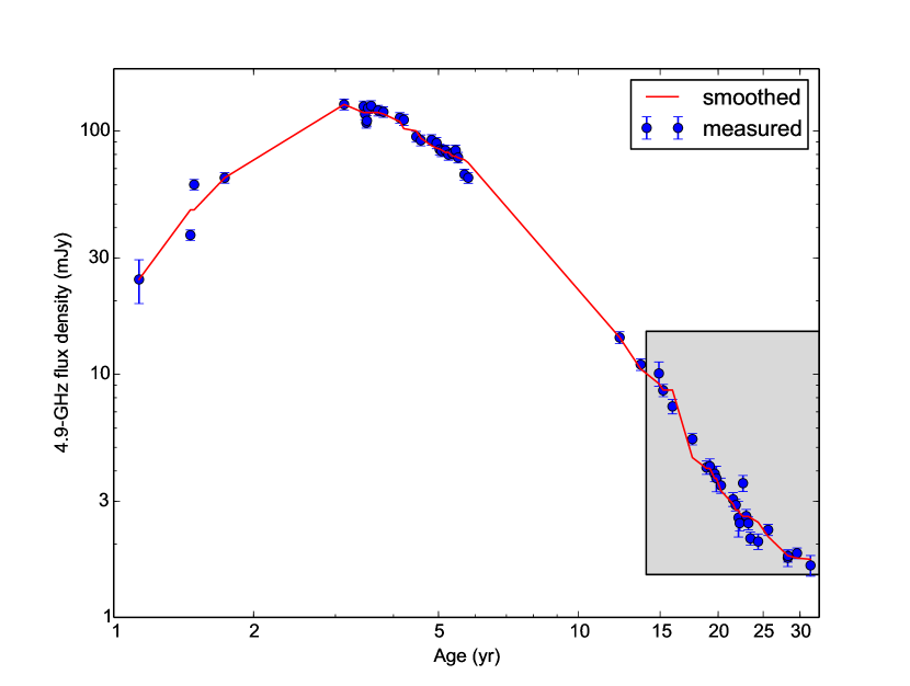
Figure 2: The complete 5-GHz lightcurve of SN 1986J, based on measurements from the present work as well as ones from Weiler et al. (1990), Paper I and Paper II. We show the measured values with their estimated standard errors in blue, and a smoothed average curve in red. The smoothing was a simple boxcar averaging in log(age) and log(flux-density), with the width of the boxcar being 20% in age. The lightly shaded rectangle shows the time interval which we use for modeling the effect of the central component on the SED.

We plot the multi-frequency flux densities at $t>14$ yr in two ways: first, in Figure 3 we plot the evolution of the flux density with time at several different frequencies for the period 1998 to 2016 ($t=15$ to 32 yr). Second, in Figure 4 we plot the SED of a number of recent epochs. In both figures, we include some earlier measurements from Paper II, and Bietenholz et al. (2004, 2005).

Figure 3: The radio lightcurves of SN 1986J at frequencies between 1.5 and 22 GHz. For clarity, the lightcurves at 8.4 GHz and 22 GHz were shifted down in flux density by factors of 3 and 10 respectively. The plotted error bars are $1\sigma$ standard errors which include both statistical and systematic contributions added in quadrature. Data are taken from this paper and Paper II, Bietenholz et al. (2005) and Bietenholz et al. (2004). In § 3, we describe our Bayesian fit to the evolving spectral energy distribution after the first appearance of the central (inverted spectrum) component at $t=14.9$ yr, and we show the fitted lightcurves using dotted lines of the same colors as were used for the measurements from the same epoch.

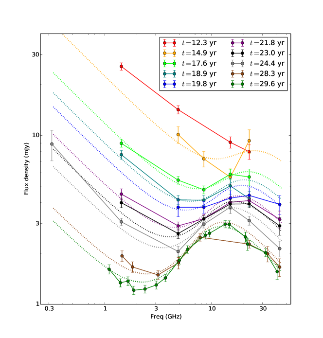
Figure 4: The evolving SED of SN 1986J. The colored points and associated solid lines show the SED at the indicated age (in years, calculated from $t_{0}=1983.2$), with the earliest one at the top. The uncertainties are estimated standard errors, with statistical and systematic contributions added in quadrature. Data are taken from this paper, Paper II and Bietenholz et al. (2004, 2005). In § 3, we describe our Bayesian fit to the evolving spectral energy distribution after the first appearance of the central (inverted spectrum) component at $t=14.9$ yr. For reference, we include the spectrum at $t=12.3$ yr, before the emergence of the central component, which was not used in our fit. We plot the fitted spectra for each subsequent epoch using dotted lines of the same colors as were used for the measurements from the same epoch. The model is fairly simple, and fits the SEDs at all epochs simultaneously with only eight free parameters, so the fit to the measured spectrum at any one epoch is only approximate, but the model should give a good overall description of the evolution.

3 Bayesian Fit to the Evolution of the Spectral Energy Distribution

3.1 Model for the Bayesian Fit

Our latest broadband SED shows that at $t=29.6$ yr, the high-frequency turnover, $\nu_{\rm peak}$, occurs at $\sim$15 GHz, while the inversion in the spectrum, $\nu_{\rm inv}$, occurs at $\sim$2 GHz. The SED from $t=29.6$ yr as well as the earlier ones are shown in Figure 4. The high-frequency turnover was not observed till $t=17.6$ yr, at which point $\mbox{$\nu_{\rm peak}$}\simeq 17$ GHz. By $t=29.6$ yr, $\nu_{\rm peak}$ had moved downwards but only slightly to $\sim$14 GHz, and so $\mbox{$\nu_{\rm peak}$}\ \propto t^{(-0.3\pm 0.3)}$. The inversion was first detected at $t=14.9$ yr at which time $\mbox{$\nu_{\rm inv}$}\simeq 15$ GHz. By $t=29.6$ yr, $\mbox{$\nu_{\rm inv}$}\simeq 2$ GHz, so the inversion point is moving downwards in frequency much more rapidly with $\mbox{$\nu_{\rm inv}$}\propto t^{(-2.9\pm 0.4)}$.

We fitted a simple model to the observations after $t=14$ yr, where the SED is modeled as a combination of two parts. The first, due to the shell, is assumed to suffer no absorption so:

$$S_{\rm shell}=S_{0,{\rm shell}}\left(\frac{t}{\rm 20\>yr}\right)^{b_{\rm shell}}\,\left(\frac{\nu}{\rm 1\>GHz}\right)^{\alpha_{\rm shell}}$$

The second, due to the central component, has an intrinsic SED of

$$S_{\rm comp}=S_{0,{\rm comp}}\left(\frac{t}{\rm 20\>yr}\right)^{b_{\rm comp}}\>\left(\frac{\nu}{\rm 1\>GHz}\right)^{\alpha_{\rm comp}}$$

but is free-free absorbed by material with an emission measure, EM $=\int{N_{e}^{2}\cdot dl}$, where $N_{e}$ is the electron number density, and $l$ is the path-length along the line of sight.

In our model, the EM is also time-variable and is given by

$$\mathrm{EM}=\mathrm{EM}_{0}\cdot\left(\frac{t}{\rm 20\ yr}\right)^{b_{\rm EM}}\,\mbox{cm${}^{-6}$~{}pc},$$

and the corresponding optical depth is

$$\tau=3.28\times 10^{-7}\,\left(\frac{\nu}{\mathrm{GHz}}\right)^{-2.1}\,\left(\frac{T_{e}}{10^{4}\,\mathrm{K}}\right)^{-1.35}\,\left(\frac{\mathrm{EM}}{\mbox{cm${}^{-6}$~{}pc}}\right).$$

We assume an electron temperature of $T_{e}=10^{4}$ K.

In the case of purely external absorption, the inverted part of the spectrum has a steep frequency dependence with $S_{\mathrm{comp,\,abs}}\propto\nu^{2.1}$, which does not well match our observed SEDs (see Figure 4 and Paper II, ). We therefore take the emitting and the absorbing material to be mixed, in which case the inverted part of the spectrum has $S_{\mathrm{comp,\,abs}}\propto\nu^{(\alpha_{\rm comp}+2.1)}$. The contribution of the partly absorbed central component is then

$$S_{\mathrm{comp,\,abs}}=S_{\rm comp}\,\tau^{-1}\,(1-e^{-\tau})$$

This model is almost certainly an oversimplification, for example the spectral indices might also be time-variable, or the time-dependence of the various quantities might not in fact be of a powerlaw form. However, the results give some physical insight into how the time-dependencies of various quantities might interact to produce the observed sequence of SEDs.

3.2 Results from the Bayesian Fit

Having thus defined our model, we then performed a Bayesian fit, and used Monte-Carlo Markov chain integration to estimate the posterior probability distribution of the eight free parameters, namely $S_{0,{\rm shell}}$, $b_{\rm shell}$, $\alpha_{\rm shell}$, $S_{0,\,{\rm comp}}$, $b_{\rm comp}$, $\alpha_{\rm comp}$, EM₀, and $b_{\rm EM}$. Further details on the Bayesian fit and a comparison to a least-squares fit are given in Appendix A.

We obtained the following values:
$S_{0,{\rm shell}}=$ $\phantom{0}7.07\pm 0.17$ mJy, $b_{\rm shell}=$ $-3.92\pm 0.07$, $\alpha_{\rm shell}=$ $-0.63\pm 0.03$, $S_{0,{\rm comp}}=$ $61\pm 17$ mJy, $b_{\rm comp}=$ $-2.07\pm 0.16$, $\alpha_{\rm comp}=$ $-0.76\pm 0.07$, EM${}_{0}=$ $(1.64\pm 0.20)\times 10^{9}$ cm^-6 pc, and $b_{\rm EM}=$ $-2.72\pm 0.26$.
The listed uncertainties are the standard deviations over the posterior distribution as determined by the Markov-Chain Monte-Carlo integration. We plot the fitted spectra (as the dotted lines) in Figure 4. Note that $S_{0,{\rm comp}}$ and $\alpha_{\rm comp}$ are highly anti-correlated (see Appendix A). The fitted flux density of the central component at 10 GHz is better constrained than $S_{0,{\rm comp}}$, and is $10.4\pm 1.1$ mJy as evaluated from the posterior distribution. Our fit suggests that the shell brightness is declining rapidly, with $S_{\rm shell}\propto t^{-3.92\pm 0.07}$. Even the central component is declining in unabsorbed flux density, with $S_{\rm comp}\propto t^{-2.07\pm 0.16}$. As can be seen in Fig. 3, the 22-GHz flux density, where the central component is mostly optically thin, continues to decline, albeit slightly more slowly than that at 1.5 GHz, which is likely still dominated by the shell. At 10 GHz and $t=20$ yr, the unabsorbed flux density of the central component is $6\pm 1$ times larger than that of the shell. The central component is declining significantly less rapidly than the shell which implies that it is becoming relatively more dominant. In other words the fraction of the emission due to the central component is increasing with time, even at frequencies where the central component is optically thin. Once the central component dominates, the total flux density decline would flatten to about $S\propto t^{-2.07}$.

The amount of absorption suffered by the central component is also decreasing with time: in our fitted model, the emission measure, EM, of the material responsible for the free-free absorption of the central component is EM $\propto t^{-2.72\pm 0.26}$. It is the declining absorption that produces the apparent increase with time of the central component’s flux density at some frequencies, in particular at 5 GHz where it has come to dominate the images in the last decade.

Since EM = $\int{N_{e}^{2}\cdot dl}$, in a system which has a constant total number of free electrons and is homologously expanding $\propto t^{q}$ (all spatial dimensions $\propto t^{q}$), one would expect EM $\propto t^{-5q}$. Our fitted value of $b_{\rm EM}$ therefore suggests a system expanding with spatial dimensions $\propto t^{0.54\pm 0.05}$. This indicates a system which is slightly more decelerated than the supernova shell, for which we measured an expansion $r_{\rm out}\propto t^{0.69\pm 0.03}$ (Paper II).

From our VLBI images, we obtained a FWHM diameter of $1.3\times 10^{17}$ cm or 0.044 pc for the central component at $t=31.6$ yr. Our fit to the SED suggests that at that time, EM $=4.7\times 10^{8}$ cm^-6 pc, implying an average $N_{e}=1.0\times 10^{5}$ cm^-3 if the absorption is internal to the central component. For a uniform sphere of fully ionized material with mass in u (unified atomic mass units) per free electron, of $\mu_{e}=1.3$, this amounts to $M_{\rm ionized}\gtrsim 0.14$ $M_{\sun}$, so the mass within the central component would be at least that amount (see §4.2 below for a discussion of the case where the absorption is not internal to the central component but rather due to the supernova ejecta).

The fitted optically-thin spectral indices for the shell and the central component were $\alpha_{\rm shell}=-0.63\pm 0.03$ and $\alpha_{\rm comp}=-0.76\pm 0.07$. Although formally these are different by $1.7\sigma$, considering the relatively simple nature of our model, it is not clear whether the difference is significant. We performed a fit to the evolving SED where we used a single spectral index, $\alpha$, for both the shell and the central component, which fit the measurements almost as well, and obtained $\alpha=-0.64\pm 0.03$. Our measurements are therefore compatible with both the shell and the central component having the same optically-thin spectral index.

Our Bayesian fit to the SEDs implies that $S_{\rm comp}=14\times S_{\rm shell}$ at $t=29.6$ y and 5 GHz (before any absorption of the central component). This can be seen in Figure 4, where extrapolation of the high-frequency part of the spectrum, i.e., the sum of shell and central component spectra, would be $\sim$14 times higher than the low-frequency part which is just from the shell.

The approximate nature of our model notwithstanding, we can therefore say that the unabsorbed flux density from the central component is at least $10\times$ higher than that of the shell at $t=29.6$ yr. From our fitted FWHM width of the central component of $\theta_{\rm comp}=900$ $\mu$as and the estimated angular radius of the shell of $\mbox{$\theta_{\rm 90\%\;flux}$}\sim$4 mas at $t=29.6$ yr (Paper III), we calculate that the component occupies $\sim$1.3% of the projected area. The central component, therefore, must have an unabsorbed brightness $>10/0.013$ or $>750$ times that of the shell at $t=29.6$ yr.

3.3 Short-term Variation in the Flux Density

The model we used for the Bayesian fit had a smoothly evolving SED. However, as can be seen from Figures 3 and 4, although our model adequately reproduces the overall shapes of the multi-frequency radio lightcurves and the evolution of the SED, the measurements do show some significant deviations from the model. In particular, the lightcurve at 22 GHz, which is dominated by the central component, seems to show larger short-term deviations from the smoothly-evolving model, suggesting perhaps some variability of the central component.

There is also some evidence for short-term deviations or flares at other frequencies. The most prominent of these is a positive excursion of the flux density by a factor of $\sim$1.4 seen at both 4.9 and 8.4 GHz at $t=22.6$ yr. There was no corresponding measurement at 1.5 GHz, and at 22-GHz only an insignificant enhancement is seen. This suggests flaring behavior with a spectrum deviating notably from a powerlaw.

4 Discussion

We have presented new, broadband measurements of SN 1986J’s SED between 1 and 44 GHz, and fitted a model to its evolution. How can we interpret the evolution of the SED, and what light does it shed on the nature of SN 1986J’s mysterious central component, which appeared in VLBI images in conjunction with a dramatic evolution in the SED?

We will proceed to discuss four different hypotheses for the origin of the central component in light of our measurements. In § 4.1, we show that the first hypothesis, which is that the central component is merely a dense condensation in the circumstellar medium (CSM), lying by chance near the projected center of the source, is unlikely. Then, in § 4.2 we discuss absorption by the ejecta, which is a common feature of the three remaining hypotheses for the origin of the central component. In § 4.3 we discuss the second hypothesis, suggested by Chevalier (2012), in which SN 1986J was the second SN resulting from a massive binary, where the compact remnant from the first SN inspirals into the second star and produces a very anisotropic CSM in which the second supernova, SN 1986J, then explodes. In § 4.4, we discuss the third hypothesis, which is that the central component is a pulsar wind nebula around the nascent neutron star which was left behind by the SN explosion. Finally, in § 4.5 we discuss the fourth hypothesis, which is that the central component is radio emission associated with a black hole left behind by the explosion.

4.1 Is the Central Component Due to a Dense Condensation in the CSM?

Is it possible that the central component is merely the result of the supernova shock interacting with a dense condensation in the CSM, which lies by chance close to the projected center, but on the near side of the source along the line of sight? If the condensation were sufficiently dense, the condensation itself could provide the necessary opacity to account for the inverted part of the spectrum and the delayed turn-on. The central location would therefore be coincidental. Given that a somewhat similar bright radio spot was seen to the SE in earlier images (; ), which is indeed thought to be due to a condensation in the CSM, such a dense condensation would not be unique.

We measured a low proper motion for the central component, consistent with being stationary, in Paper III. Such low proper motion is expected for a CSM condensation unless its structure and placement deviates strongly from symmetry along the line of sight.

In this scenario, one would expect the central component to fade after the shock has progressed through it. The central component was first seen at $t=14.9$ yr, when the supernova was only 60% of its present size, and it is still getting brighter. Given that the condensation would have to be quite dense, the portion of the shock traversing the condensation would slow considerably compared to the remainder, and for sufficiently high densities, lifetimes of a few decades would not be excluded. Since the central component is still brightening relative to the shell, the shock would probably not have traversed more than half of the putative CSM clump. We measured a sky-plane radius for the central component of $6.7\times 10^{17}$ cm (Paper III). Assuming a spherical clump, and given that the central component has been visible since $t=14$ yr, we can calculate that the shock speed within the clump would have to be $<1300$ km s^-1, which is $\lesssim$23% of the speed of the parts of the shock unaffected by the central component of $\sim$5700 km s^-1 ($t=15.9-25.6$ yr, Paper II, ). This would necessitate quite high densities in the clump.

The high surface brightness (before absorption) of $\gtrsim 750$ times that of the remainder of the shell, seems hard to accommodate in this scenario. When the shock traverses a density jump in the CSM, brightness changes on the same order as the magnitude of the jump in density are expected, suggesting that the clump should have a density $\gtrsim 750$ times that of the remainder of the CSM at that radius. Given the average densities expected from mass loss at a rate of $4\sim 10\times 10^{-5}\mbox{$M_{\sun}$~{}yr${}^{-1}/10$~{}km~{}s${}^{-1}$}$ of $(5\sim 13)\times 10^{22}$ g cm^-3 (Paper II), we would therefore expect number densities in the clump of $(3\sim 7)\times 10^{-19}$ g cm^-3, or, assuming atomic H, number densities of $2\sim 4\times 10^{5}$ cm^-3.

A clumpy CSM has been suggested for SN 1986J with shocks driven into dense clumps in the CSM explaining both the X-ray emission and low line velocities (Chugai, 1993). Clumps with similarly high number densities have been suggested in the CSM of other SNe, for example values in excess of $10^{6}$ cm^-3, even higher than we surmised for a putative CSM condensation in SN 1986J, have been suggested in SN 2006jd and SN2010jl (Smith et al., 2009; Fransson et al., 2014, respectively). However, the number of such clumps is thought to be large ($\sim$1000), their sizes small ($\sim 3\times 10^{15}$ cm), and their filling factor low, ($\sim$0.005), very much in contrast to what we find for SN 1986J. A clumpy CSM therefore would be unable to explain either the fact that we see only a single bright spot in SN 1986J or its longevity.

4.2 Absorption by the Supernova Ejecta

If the central component is not a fortuitously-placed clump in the CSM, near the center only in projection, then it is in (or close to) the physical center of the expanding supernova. The absorption of its radio emission at low frequencies would then be due to free-free absorption by the intervening supernova ejecta along the line of sight.

Can we deduce anything about the ejecta from our radio observations? In our Bayesian model of the evolving SED we found that the best fit had a time-dependent emission measure of

$${\rm EM}(t)=(1.64\pm 0.21)\times 10^{9}\cdot\left(\frac{t}{\rm\,20\,yr}\right)^{-2.72\pm 0.26}\;\mbox{cm${}^{-6}$~{}pc}.$$

4.2.1 Uniformly Distributed Free Electrons

If we assume that the thermal free electrons responsible for the EM are uniformly distributed out to the reverse shock, which we take to be at 80% of the outer radius of the SN (taken from our fit in Paper II, ), and therefore to be at $4.3\times 10^{17}$ cm at $t=20$ yr, then we can calculate that the average value for $N_{e}$ must be $1.1\times 10^{5}$ cm^-3. If we assume a uniform distribution of matter and $\mu_{e}=1.3$, this implies a mass of $\sim$40 $M_{\sun}$ of fully ionized matter. This is higher than is reasonable, so we must conclude that the density distribution of the absorbing matter is non-uniform.

As shown by Chevalier & Fransson (1994), the ejecta are not expected to be uniformly ionized, instead, probably only the outer portion of the ejecta, nearest the reverse shock, will be highly ionized. The total amount of ionized material in the ejecta of a SN, $M_{\rm ion}$, is not well known: $M_{\rm ion}$ depends on the poorly-known ionization fraction and distribution of the ionized material in the ejecta. It is expected that the ejecta will cool and become neutral except for a shell which is heated by emission from the shocks (Chevalier & Fransson, 1994), so $M_{\rm ion}$ is likely to be only a fraction of the total ejecta mass. The expected value of $M_{\rm ion}$ for SN 1986J is likely in the range of 0.5 to 5 $M_{\sun}$. Zanardo et al. (2014) argues that $M_{\rm ion}$ in the ejecta of SN 1987A is in the range of 0.7 to 2.5 $M_{\sun}$, and since SN 1986J’s progenitor was probably more massive than that of SN 1987A, we consider values of $M_{\rm ion}$ up to 5 $M_{\sun}$, and consider values larger than that unlikely.

4.2.2 Non-Uniformly Distributed Free Electrons

By making some assumptions about the shape of the ionized region within the ejecta, we can constrain the distribution of ionized matter using our fitted values of EM. If we assume spherical symmetry, then the ionized matter must be distributed in a region in the shape either of a spherical shell or a sphere. We consider both possibilities. First, a spherical shell, bounded on the outside at radius $r_{\rm rev.\;shock}$ by the reverse shock, based on the expectation that the ejecta will be ionized from the outside by the shock. Second, a spherical region in the interior of the ejecta, extending out to some radius $<\mbox{$r_{\rm rev.\;shock}$}$. The EM then depends on $M_{\rm ion}$ and the path-length through the ionized matter (and also, but only weakly, on $\mu_{e}$, and we assume again that $\mu_{e}$ = 1.3 for the ejecta). The path-length is the thickness of the shell or the radius of the sphere in the two cases.

In Figure 5 we plot the value of $M_{\rm ion}$ required to produce the EM of $1.64\pm 0.21\times 10^{9}$ cm^-6 pc as a function of the path-length for our two chosen distributions, with the value of the EM being the one we found for SN 1986J at $t=20$ yr.

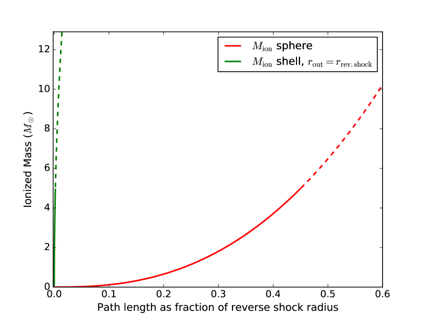
Figure 5: The ionized mass ($M_{\rm ion}$) in the ejecta of SN 1986J for an emission measure (EM) through the ejecta of $1.64\times 10^{9}$ cm^-6 pc, as a function of path-length, which we express in fractions of the reverse shock radius, $r_{\rm rev.\;shock}$. The value of EM is the one we found for SN 1986J at $t=20$ yr (see text, § 3.2). We assume a mass per free electron, $\mu_{e}$ of 1.3 u. The green line near the left edge shows $M_{\rm ion}$ for ionized matter distributed in a spherical shell extending out to $r_{\rm rev.\;shock}$, with the path-length being the thickness of the shell, while the red line shows $M_{\rm ion}$ for a spherical distribution of ionized matter, extending out to so some $r<\mbox{$r_{\rm rev.\;shock}$}$, with the path-length being the radius of the sphere. We consider $M_{\rm ion}$ = 5 $M_{\sun}$ to be a reasonable upper limit for the total amount of ionized matter in SN 1986J, and we plot values of $M_{\rm ion}$$>5$ using dashed lines. For a spherical shell, only very thin shells (thickness $<0.002\,\mbox{$r_{\rm rev.\;shock}$}$) are possible.

As can be seen, an ionized region near the reverse shock cannot produce our value of EM except in the case of large mass $M_{\rm ion}$ concentrated in a very thin shell, for example $M_{\rm ion}$= 5 $M_{\sun}$ in a shell of thickness only 0.002 times the reverse shock radius, or $9\times 10^{14}$ cm. Such a large mass within such a very thin shell seems improbable.

If the ejecta are ionized from the center of the supernova, then a spherical region of ionized ejecta can easily produce the required value of EM, with, for example, $M_{\rm ion}$= 2 $M_{\sun}$ in a region with a radius of $0.3\times$ that of the reverse shock, or $1.3\times 10^{17}$ cm.

Our value of EM depends on an assumed electron temperature of $T_{e}=10^{4}$ K. Could the required absorption be produced if $T_{e}$ were in fact substantially different? Lower values of $T_{e}$ would increase the absorption, and thus lower the ionized mass, i.e. the value of $M_{\rm ion}$, required, however, such low values would likely not be associated with sufficient ionization to produce the free electrons required for the absorption. Higher values of $T_{e}$ would only increase the value $M_{\rm ion}$ required.

The value of the EM from the ejecta is very sensitive to the radial distribution of the ionized ejecta. The density distribution in the interior part of the ejecta is much flatter than the steep profile in the outside regions, but nonetheless probably not constant with radius. Density distributions with $\rho\propto r^{n}$ with $n\sim-1$ are expected (e.g., Matzner & McKee, 1999). For any density distribution with $n<-0.5$, the formal value of the EM becomes infinite near $r=0$. For inner radii small compared to the outer radius, however, our conclusions above are not much altered: if, for example, we take a $\rho\propto r^{-1}$ density distribution extending inward from $0.25\times$ the reverse shock radius ($1.9\times 10^{17}$ cm at $t=20$ yr) to the radius we measured for the central component of $6.7\times 10^{16}$ cm, we find that our fitted value of EM can be produced with $\mbox{$M_{\rm ion}$}=1.5$ $M_{\sun}$.

Our conclusion, that producing the value of the EM we observed for the central component requires that the absorbing ionized material be concentrated in the inner part of SN 1986J, therefore seems robust. Unless $M_{\rm ion}$ is so concentrated, unreasonably large total masses ($>5$ $M_{\sun}$) are required to produce the observed absorption. The only other way to produce the observed absorption would be to have a few $M_{\sun}$ distributed in a very thin shell near the reverse shock which we consider unlikely, or of course to have $M_{\rm ion}$ not spherically distributed, which would imply that our particular line of sight suffers from much higher absorption than most. Our value of EM also places some constraints on the associated dispersion measure, but we defer discussion of dispersion measure and the implications for fast radio bursts to a companion paper: Bietenholz & Bartel (2017a).

4.3 Is the Central Component Due to a Common-Envelope Evolution of SN 1986J’s Progenitor?

The first hypothesis for origin of the bright central component was recently suggested by Chevalier (2012). In this hypothesis, Type IIn supernovae, such as SN 1986J, arise from massive-star binary systems that have undergone a period of common-envelope (CE) evolution after the first star in the system exploded as a supernova. SNe resulting from massive binary systems are not unexpected since a large fraction of massive stars is expected to be in binaries (Sana et al., 2012). The explosion of the first star, not observed in the case of SN 1986J, leaves behind a compact object (neutron star or black hole), and a subsequent CE phase results in the inspiral of the compact object into the second star. The CE phase causes a period of very strong and highly anisotropic mass loss, which is followed by the second, observed supernova explosion (for a more elaborate, triple-star version of this scenario, see Justham et al., 2014). The result is a highly anisotropic CSM, much denser in the equatorial plane of the binary than elsewhere.

If SN 1986J originates from such a system, then after the explosion, part of the shock expands relatively rapidly through the lower density polar regions, producing the observed “shell” component, but another part of the shock interacts with the very dense equatorial CSM, expanding much more slowly and producing the observed central component. The density contrast between the equatorial and the polar CSM can be more than an order of magnitude (Ricker & Taam, 2012). The shock has something like an hourglass shape with the central component representing the narrow waist of the hourglass, with our line of sight being intermediate between a polar and an equatorial one. The ejecta are initially opaque to radio waves, so the ejecta which expand above and below the equatorial disk will initially free-free absorb any emission from the part of the shock in the disk. Only after some time do the bulk of the ejecta expand, fragment or recombine to the point where the central disk can be seen, at which point the radio central component “turns on.”

Is this hypothesis consistent with our observations? We showed in § 4.2 above that the observed amount of absorption of the central component, i.e., the part of the shock interacting with the putative dense equatorial disk, was compatible with what would be expected from a few $M_{\sun}$ of ionized supernova ejecta. Although the shock and the ejecta have a non-spherical structure, the system might be expected to expand in an approximately homologous manner, albeit with the portion of the shock in the dense equatorial disk traveling much more slowly than the rest. Our observations of the evolving SED are in fact approximately consistent with a homologously expanding system. We also find that the emission from the central component and from the shell have approximately the same optically thin spectral index, which is also expected in this case.

We further found in § 4.2 that the ionized material responsible for the absorption seen towards the central component is most likely near the center of the SN, rather than being out towards the outer edge of the SN. Such concentration near the center is also expected in the case of a highly anisotropic CSM resulting from CE evolution, since the dense, ionized material would also be near the narrow waist of the hourglass.

The CE hypothesis therefore seems broadly consistent with our observations, although modeling of the CE scenario, against which we could compare our observations in detail, has not been carried out to date, and none of our VLBI images obviously suggest an hour-glass morphology.

4.4 Is the Central Component a Pulsar Wind Nebula?

The second hypothesis is that the central component is an emerging pulsar wind nebula (PWN), forming around the neutron star left behind in the supernova explosion. In this case, the central location and its low proper motion are readily explained.

A PWN is expected to expand with velocities in the range of 1000 to 2000 km s^-1, and to have a size of 5 to 20% of that of the forward shock at ages of a few decades. This size is consistent with our measurement of the central component’s radius (HWHM) of $\sim$9% of the shell radius at $t=31.6$ yr (Paper III).

The 20-GHz flux density of the central component at $t=30$ yr was $\sim$2 mJy (see Figure 4), corresponding to a spectral luminosity of $\sim 3.3\times 10^{26}$ erg s^-1 Hz^-1, or a luminosity ($\nu L_{\nu}$) of $6.6\times 10^{36}$ erg s^-1, which is $\sim$120 times the current value for the $\sim$1000-yr old Crab Nebula (see, e.g., Bietenholz et al., 1997). The spindown power of young pulsars is expected to be $\gtrsim 10^{39}$ erg s^-1, several orders of magnitude higher than the above luminosity, and thus easily able to power the putative PWN. The spindown power is expected to be constant or decay only slowly with time (e.g., Kotera et al., 2013; Chevalier & Fransson, 1992). Gelfand et al. (2009) modeled the evolution of a PWN and predicted radio luminosities comparable to that observed for SN 1986J’s central component at $t=20$ yr. In their model, the radio luminosity of the PWN decays relatively slowly, approximately as $t^{-0.5}$, for the first few decades. Although we indeed found that the radio luminosity of the central component is decaying with time, it seems to be decaying significantly faster ($S_{\rm comp}\propto t^{-2.07\pm 0.16}$) than suggested by Gelfand et al. (2009)’s model of PWN.

The optically-thin spectral index of the central component was $-0.76\pm 0.07$, which is considerably steeper than observed in any known PWN, which have spectral indices in the range $-0.3$ to 0.0 (Gaensler & Slane 2006; see also Green 2014). We further found that the decrease of the absorption of the central component suggested a system that was decelerated perhaps slightly more than the shell, which is already significantly decelerated in SN 1986J (with $r\propto t^{0.69}$ Paper II, ). One would expect a PWN, by contrast, to be somewhat accelerated, since the PWN is driven into the still freely expanding ejecta interior to the decelerated forward shock (e.g., Chevalier & Fransson, 1992; Gelfand et al., 2009; Bietenholz & Nugent, 2015).

On the balance, the observations do not favor a PWN explanation, although little enough is known about young PWN that such an explanation cannot be decisively ruled out.

4.5 Is the Central Component Due to a Newly Formed Black Hole?

The third hypothesis is that the central component is due to a newly formed black hole. The progenitor of SN 1986J was thought to be massive (Rupen et al., 1987; Weiler et al., 1990) and might therefore have produced a black hole instead of a neutron star. Could the central component be radio emission originating from a black hole environment, specifically in the form of jets powered by fallback accretion? We note that the accretion could occur onto a neutron star as well as onto a black hole but, as we explain below, we consider this possibility less likely.

Radio emitting jets in accreting black-hole systems can have a wide range of radio spectra, due to the possible presence of both self-absorbed and optically thin components, so the central component’s observed optically thin spectrum can easily be accommodated by this hypothesis. The slightly higher short-term variability at 22-GHz noted in § 3.3 is also expected in this case.

However, SN 1986J’s central component is far more radio-luminous than any known stellar-mass black hole system: at $t=30$ yr, the central component has a measured radio luminosity of $L_{\rm R}$= $3\times 10^{35}$ erg s^-1 ($\nu L_{\nu}$), with the unabsorbed value being about an order of magnitude larger (§ 4.2). Known accreting stellar-mass black hole systems in X-ray binaries have $\mbox{$L_{\rm R}$}\lesssim 10^{32}$ erg s^-1 (see, e.g., Körding et al., 2006). Of course, an accreting black hole could have a wide range of $L_{\rm R}$ depending on the accretion rate, and one in SN 1986J may be accreting at a much higher rate than any of those in X-ray binaries.

The X-ray emission in accreting black holes is generally correlated with the radio emission. Can we therefore constrain a possible accreting black hole in SN 1986J using X-ray observations? Indeed, in the case of the Type IIL SN 1979C, a flattening of the X-ray lightcurve at a luminosity comparable to $L_{\rm Edd}$ has been interpreted in terms of a newly formed black hole (Patnaude et al., 2011). However, no clear central component has been seen in the radio in SN 1979C (Bartel & Bietenholz, 2008). Furthermore, Dwarkadas & Gruszko (2012) show that SN 1979C’s flat X-ray lightcurve, as well as those of some Type IIn SNe, could be due to circumstellar interaction rather than a central black hole.

In any case, the X-ray lightcurve of SN 1986J does not seem to be particularly flat: X-ray observations have been obtained at various times between $t\simeq 8.5$ yr and 20.6 yr (1991 and 2003), and Houck (2005) found that the X-ray flux (0.5 to 2.5 keV) was declining with time $\propto t^{-1.7\pm 0.25}$, consistent with CSM interaction. No more recent X-ray measurements have been published.

Houck (2005) found that the unabsorbed X-ray luminosity, $L_{\rm X}$, at $t=20.6$ yr was $1.9\times 10^{39}$ erg s^-1 (0.5 to 2.5 keV), equal to the Eddington luminosity $L_{\rm Edd}$ of a 16 $M_{\sun}$ black hole. While this value is possible for an accreting black hole, it is larger than expected for long-lasting fallback accretion (Perna et al., 2014).

It has been observed that the $L_{\rm R}$, $L_{\rm X}$, and the black-hole mass for accreting black holes are related and lie on a “fundamental plane” (see, e.g., Ho, 2008; Falcke et al., 2004; Merloni et al., 2003). The relationship holds for a wide range of masses from stellar mass black holes in Galactic X-ray binaries through supermassive ones in the centers of galaxies. If the emission from the center of SN 1986J is due to an accreting black hole, can we place it on this fundamental plane? Merloni et al. (2003) gives a plot of the projected fundamental plane, with an X-axis of $0.60\log(\mbox{$L_{\rm X}$})+0.78\log(M)$, where $L_{\rm X}$ is in erg s^-1 and $M$ is the black hole mass in $M_{\sun}$. If we assume that all the X-ray emission at $t\sim 20.7$ yr is due to the central component, its $L_{\rm X}$ would be $1.9\times 10^{39}$ erg s^-1. If we further take a relatively high black hole mass of 20 $M_{\sun}$, we find that the fundamental plane relationship predicts that $\mbox{$L_{\rm R}$}\simeq 3\times 10^{31}$ erg s^-1. This is almost 4 orders of magnitude fainter than the measured $L_{\rm R}$ of the central component at that age ($\sim 3\times 10^{35}$ erg s^-1). In fact, given that there is significant absorption by the ejecta at 5 GHz, the intrinsic $L_{\rm R}$ is likely higher by up to an order of magnitude. A mass much above 20 $M_{\sun}$ also seems unlikely. Although there is considerable scatter in the fundamental plane relationship, SN 1986J’s central component seems to have a far higher ratio of $L_{\rm R}$/$L_{\rm X}$ than accreting black holes which are on the fundamental plane, in fact far higher than any known stellar-mass black hole systems. It might be expected that a black hole as young as one in SN 1986J would accrete at a much higher rate than the much older Galactic X-ray binaries, but high accretion rates seem to quench the radio emission rather than enhance it (e.g., Fender et al., 2010). SN 1986J’s high radio luminosity, and in particular, its high ratio of $L_{\rm R}$/$L_{\rm X}$, seem discrepant with that seen in other accreting black hole systems.

As noted above, the accreting object could in fact be a neutron star rather than a black hole, as accreting neutron stars can also power jets and produce radio emission. However, for the same X-ray luminosity, neutron-star systems tend to have lower radio luminosities than black-hole systems (Körding, 2014), so we consider an accreting neutron star less likely than a black hole.

In summary, the clearly distinct, stationary central compact radio component could be interpreted in terms of an accreting black-hole system. As we noted in Paper III, the hotspot to the NE is approximately aligned with the extension of the central component, which, although quite inconclusive, could be interpreted in terms of a jet structure. However, although they do not rule out the black-hole hypothesis, the high radio luminosity, the declining X-ray lightcurve and the large ratio of $\mbox{$L_{\rm R}$}/\mbox{$L_{\rm X}$}$ argue against it.

5 Summary and Conclusions

We obtained new multi-frequency VLA flux density measurements of SN 1986J, made in conjunction with VLBI observations, which showed the continued evolution of its spectral energy distribution. We found that:

1. The radio spectral energy distribution shows both an inversion and a high frequency turnover. Between these two points, the emission increases with increasing frequency. The inverted part of the spectrum is due to the central component, which is absorbed at low frequencies thus producing the high-frequency turnover. At frequencies below the inversion, the shell emission dominates. The inversion is presently near 2 GHz, and the high-frequency turnover near 15 GHz, and both the inversion and turnover are progressing downward in frequency with time.

2. We performed a Bayesian fit of a model consisting of a shell and a partly absorbed central component to the evolving spectrum. The fit suggests that the optically thin, or intrinsic, spectral indices of the central component and the shell radio emission are consistent with being the same (at $\alpha\simeq-0.64$). At $t=20$ yr, the absorption of the central component is produced by material with an emission measure of $(1.64\pm 0.20)\times 10^{9}$ cm^-6 pc which is decreasing with time $\propto t^{-2.72\pm 0.26}$. The unabsorbed flux densities of both the central component and the shell are decreasing with time, although that of the central component is decreasing less rapidly, hence the central component becomes ever more dominant. The evolution of the spectrum is approximately consistent with a system with a constant mass and ionization fraction expanding homologously with the same $r\propto t^{0.69}$ that is observed for the shell with VLBI.

3. The central component is unlikely to be due to a dense condensation in the CSM, central only in projection, due to its high surface brightness and its long lifetime. It is therefore almost certainly in the physical center of the expanding shell of ejecta. 4. The ionized material responsible for the radio absorption seen towards the central component must be distributed non-uniformly. To provide the necessary absorption with less then 5 $M_{\sun}$ of ionized material in a spherically-symmetric distribution probably requires that the ionized material be concentrated towards the center of SN 1986J, and not near the reverse shock. 5. The central component could be explained by SN 1986J being the second supernova in a binary system, with SN 1986J’s ejecta interacting with an aspherical region of very dense mass-loss from the progenitor which arose during period of common-envelope binary evolution when the compact remnant of the first supernova was within the envelope of SN 1986J’s progenitor. The central component in this picture is due to the part of the supernova shock which is interacting with the disk of very dense CSM produced resulting from the common-envelope phase, while the remainder of the shell is due to less equatorial parts of the shock which interact with the more normal supergiant wind. 6. The central component could be due to a young pulsar wind nebula, however, the steep intrinsic spectrum and the relatively rapid decay with time of its unabsorbed flux density is not consistent with what is expected. 7. The central component might be due to a newly-formed accreting black hole in the center of SN 1986J. However, it has a far higher radio luminosity, both absolutely and in comparison to the X-ray luminosity, than any known stellar-mass black-hole systems. On the other hand, not much is known about the characteristics of newly-formed black holes in supernovae.

Appendix A Details of Bayesian Fit and Comparison to Least-Squares Fit

We performed a Bayesian analysis and fitted a simple model of the evolution of the SED to our flux-density measurements. The model has eight free parameters, described in § 3.1, namely $S_{0,{\rm shell}},\,b_{\rm shell},\alpha_{\rm shell},\,S_{0,\,{\rm comp}},\,b_{\rm comp},\,\alpha_{\rm comp}$, EM₀, and $b_{\rm EM}$. We performed a Monte-Carlo Markov chain integration to estimate the posterior probability distribution of the free parameters given our flux density measurements (both ones listed in Table 1 and earlier ones). We used the PyMC package, version 2.3, by C. Fonnesbeck et al., which is available at http://pymc-devs.github.io/pymc/README.html. We give the prior distributions used for each parameter in Table 2.

The mean values and standard deviations over the posterior distributions were given in § 3.2, but we repeat them in Table 2 for convenience. We show the details of the posterior distributions in a “corner plot” in Figure 6. We also performed a weighted least-squares fit of the model to the measurements, and we obtained the results also listed in Table 2. The means over the Bayesian posterior distributions, which we use as our estimators, are consistent well within $1\sigma$ with the least-squares best-fit values, as is expected since our prior distributions are largely uninformative.

The fitted values for $S_{0,{\rm comp}}$ and $\alpha_{\rm comp}$ are strongly anti-correlated, but this is largely due to our use of a low nominal frequency of 1 GHz for $S_{0,{\rm comp}}$. Since the low-frequency flux-density is dominated by that of the shell, our measurements only poorly constrain the flux density of the central component at 1 GHz ($S_{0,{\rm comp}}$). At 10 GHz, where the central component is more dominant, the measurements constrain the flux density of the central component much more accurately. Therefore low values of $S_{0,{\rm comp}}$ in conjunction with flat values of $\alpha_{\rm comp}$, or high values of $S_{0,{\rm comp}}$ in conjunction with steep values of $\alpha_{\rm comp}$ are both possible. The flux density of the central component at 10 GHz is thus more narrowly constrained than our value of $S_{0,{\rm comp}}$ at 1 GHz of $61\pm 17$ mJy might suggest: examining the posterior distribution of the central component’s flux density at 10 GHz, we obtain a mean value of $10.4\pm 1.1$ mJy.

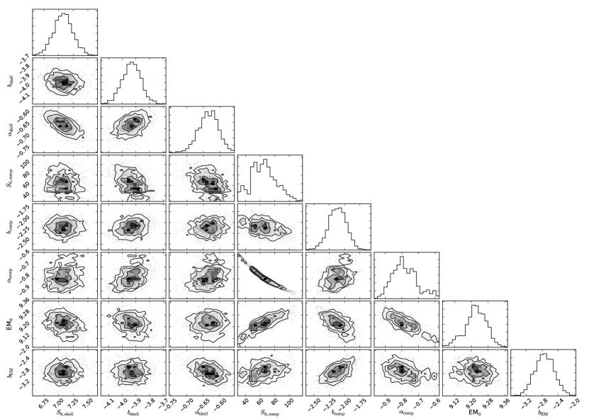
Figure 6: Joint posterior distribution (“corner plot”) of the fitted parameters. The top plot in each column gives the marginal posterior distribution of the fitted variable, while the remainder show scattergrams showing the correlation between pairs of the fitted parameters. The contours in the scatter plots are drawn at the 1, 2, and 3$\sigma$ points in the distribution. The plot was made with the “corner.py” package (Foreman-Mackey, 2016).

Table 2: Comparison of Bayesian and Least-Squares Estimates

Parameter	Prior Distribution	Bayesian fit posterior mean	Least squares best-fit	Units
		and standard deviation	and standard error
S_0,shell	uniform, 3 to 20	7.07 ±0.17	7.08 ±0.17	mJy
b_shell	uniform, $-5$ to $-2$	-3.92 ±0.07	-3.92 ±0.08	$\cdots$
α_shell	normal, mean=$-0.6,\sigma=1$	-0.63 ±0.03	-0.63 ±0.03	$\cdots$
S_0,comp	uniform, 5 to 200	61 ±17	60 ±19	mJy
b_comp	uniform, $-4$ to +1	-2.07 ±0.16	-2.11 ±0.16	$\cdots$
α_comp	normal, mean=$-0.6,\sigma=1$	-0.76 ±0.07	-0.77 ±0.08	$\cdots$
EM_0	log-uniform, 0.1 to 10	1.64 ±0.20	1.64 ±0.22	$\times 10^{9}$ cm-6 pc
b_EM	uniform, $-5$ to $-1$	-2.72 ±0.26	-2.76 ±0.26	$\cdots$

References

- Baars et al. (1977) Baars, J. W. M., Genzel, R., Pauliny-Toth, I. I. K., & Witzel, A. 1977, A&A, 61, 99
- Bartel & Bietenholz (2008) Bartel, N., & Bietenholz, M. F. 2008, ApJ, 682, 1065
- Bartel & Bietenholz (2014) Bartel, N., & Bietenholz, M. F. 2014, in IAU Symposium, Vol. 296, Supernova Environmental Impacts, ed. A. Ray & R. A. McCray, 53–57
- Bietenholz (2014) Bietenholz, M. 2014, in 12th European VLBI Network Symposium and Users Meeting (2014), published by SISSA, Trieste, ed. A. Tarchi, M. Giroletti, & L. Feretti, 51
- Bietenholz & Bartel (2007) Bietenholz, M. F., & Bartel, N. 2007, ApJ, 665, L47
- Bietenholz & Bartel (2017a) —. 2017a, ArXiv e-prints, arXiv:1707.07746
- Bietenholz & Bartel (2017b) —. 2017b, ApJ, 839, 10
- Bietenholz et al. (2002) Bietenholz, M. F., Bartel, N., & Rupen, M. P. 2002, ApJ, 581, 1132
- Bietenholz et al. (2004) —. 2004, Science, 304, 1947
- Bietenholz et al. (2005) —. 2005, Advances in Space Research, 35, 1052
- Bietenholz et al. (2010) —. 2010, ApJ, 712, 1057
- Bietenholz et al. (1997) Bietenholz, M. F., Kassim, N., Frail, D. A., et al. 1997, ApJ, 490, 291
- Bietenholz & Nugent (2015) Bietenholz, M. F., & Nugent, R. L. 2015, MNRAS, 454, 2416
- Chevalier (1987) Chevalier, R. A. 1987, Nature, 329, 611
- Chevalier (2012) —. 2012, ApJ, 752, L2
- Chevalier & Fransson (1992) Chevalier, R. A., & Fransson, C. 1992, ApJ, 395, 540
- Chevalier & Fransson (1994) —. 1994, ApJ, 420, 268
- Chugai (1993) Chugai, N. N. 1993, ApJ, 414, L101
- Dwarkadas & Gruszko (2012) Dwarkadas, V. V., & Gruszko, J. 2012, MNRAS, 419, 1515
- Falcke et al. (2004) Falcke, H., Körding, E., & Markoff, S. 2004, A&A, 414, 895
- Fender et al. (2010) Fender, R. P., Gallo, E., & Russell, D. 2010, MNRAS, 406, 1425
- Fonnesbeck et al. (2015) Fonnesbeck, C., Patil, A., Huard, D., & Salvatier, J. 2015, PyMC: Bayesian Stochastic Modelling in Python, Astrophysics Source Code Library, ascl:1506.005
- Foreman-Mackey (2016) Foreman-Mackey, D. 2016, The Journal of Open Source Software, 1, doi:10.21105/joss.00024
- Fransson et al. (2014) Fransson, C., Ergon, M., Challis, P. J., et al. 2014, ApJ, 797, 118
- Gaensler & Slane (2006) Gaensler, B. M., & Slane, P. O. 2006, ARA&A, 44, 17
- Gelfand et al. (2009) Gelfand, J. D., Slane, P. O., & Zhang, W. 2009, ApJ, 703, 2051
- Green (2014) Green, D. A. 2014, Bulletin of the Astronomical Society of India, 42, 47
- Greisen (2003) Greisen, E. W. 2003, in Astrophysics and Space Science Library, Vol. 285, Information Handling in Astronomy - Historical Vistas, ed. A. Heck, 109
- Ho (2008) Ho, L. C. 2008, ARA&A, 46, 475
- Houck (2005) Houck, J. C. 2005, in X-Ray and Radio Connections (eds. L.O. Sjouwerman and K.K Dyer). Published electronically by NRAO, http://www.aoc.nrao.edu/events/xraydio, held 3-6 February 2004 in Santa Fe, New Mexico, USA, (E3.03) 6 pages
- Justham et al. (2014) Justham, S., Podsiadlowski, P., & Vink, J. S. 2014, ApJ, 796, 121
- Körding (2014) Körding, E. 2014, Space Sci. Rev., 183, 149
- Körding et al. (2006) Körding, E., Falcke, H., & Corbel, S. 2006, A&A, 456, 439
- Kotera et al. (2013) Kotera, K., Phinney, E. S., & Olinto, A. V. 2013, MNRAS, 432, 3228
- Matzner & McKee (1999) Matzner, C. D., & McKee, C. F. 1999, ApJ, 510, 379
- McMullin et al. (2007) McMullin, J. P., Waters, B., Schiebel, D., Young, W., & Golap, K. 2007, in Astronomical Society of the Pacific Conference Series, Vol. 376, Astronomical Data Analysis Software and Systems XVI, ed. R. A. Shaw, F. Hill, & D. J. Bell, 127
- Merloni et al. (2003) Merloni, A., Heinz, S., & di Matteo, T. 2003, MNRAS, 345, 1057
- Milisavljevic et al. (2008) Milisavljevic, D., Fesen, R. A., Leibundgut, B., & Kirshner, R. P. 2008, ApJ, 684, 1170
- Mulcahy (2014) Mulcahy, D. D. 2014, Ph.D. Thesis
- Patnaude et al. (2011) Patnaude, D. J., Loeb, A., & Jones, C. 2011, New A, 16, 187
- Perley & Butler (2013) Perley, R. A., & Butler, B. J. 2013, ApJS, 204, 19
- Perna et al. (2014) Perna, R., Duffell, P., Cantiello, M., & MacFadyen, A. I. 2014, ApJ, 781, 119
- Ricker & Taam (2012) Ricker, P. M., & Taam, R. E. 2012, ApJ, 746, 74
- Rupen et al. (1987) Rupen, M. P., van Gorkom, J. H., Knapp, G. R., Gunn, J. E., & Schneider, D. P. 1987, AJ, 94, 61
- Sana et al. (2012) Sana, H., de Mink, S. E., de Koter, A., et al. 2012, Science, 337, 444
- Smith et al. (2009) Smith, N., Silverman, J. M., Chornock, R., et al. 2009, ApJ, 695, 1334
- Temple et al. (2005) Temple, R. F., Raychaudhury, S., & Stevens, I. R. 2005, MNRAS, 362, 581
- Tinyanont et al. (2016) Tinyanont, S., Kasliwal, M. M., Fox, O. D., et al. 2016, ApJ, 833, 231
- Turtle et al. (1987) Turtle, A. J., Campbell-Wilson, D., Bunton, J. D., et al. 1987, Nature, 327, 38
- van Gorkom et al. (1986) van Gorkom, J., Rupen, M., Knapp, G., et al. 1986, IAU Circ., 4248, 1
- Weiler et al. (2002) Weiler, K. W., Panagia, N., Montes, M. J., & Sramek, R. A. 2002, ARA&A, 40, 387
- Weiler et al. (1990) Weiler, K. W., Panagia, N., & Sramek, R. A. 1990, ApJ, 364, 611
- Zanardo et al. (2014) Zanardo, G., Staveley-Smith, L., Indebetouw, R., et al. 2014, ApJ, 796, 82