Parameterized Approximation Algorithms for
Bidirected Steiner Network Problems

Abstract

The Directed Steiner Network (DSN) problem takes as input a directed graph $G=(V,E)$ with non-negative edge-weights and a set ${\mathcal{D}}\subseteq V\times V$ of $k$ demand pairs. The aim is to compute the cheapest network $N\subseteq G$ for which there is an $s\to t$ path for each $(s,t)\in{\mathcal{D}}$. It is known that this problem is notoriously hard as there is no $k^{1/4-o(1)}$-approximation algorithm under Gap-ETH, even when parametrizing the runtime by $k$ [Dinur & Manurangsi, ITCS 2018]. In light of this, we systematically study several special cases of DSN and determine their parameterized approximability for the parameter $k$.

For the bi-DSN${}_{\textsc{Planar}}$ problem, the aim is to compute a solution $N\subseteq G$ whose cost is at most that of an optimum planar solution in a bidirected graph $G$, i.e., for every edge $uv$ of $G$ the reverse edge $vu$ exists and has the same weight. This problem is a generalization of several well-studied special cases. Our main result is that this problem admits a parameterized approximation scheme (PAS) for $k$. We also prove that our result is tight in the sense that (a) the runtime of our PAS cannot be significantly improved, and (b) no PAS exists for any generalization of bi-DSN${}_{\textsc{Planar}}$, under standard complexity assumptions. The techniques we use also imply a polynomial-sized approximate kernelization scheme (PSAKS). Additionally, we study several generalizations of bi-DSN${}_{\textsc{Planar}}$ and obtain upper and lower bounds on obtainable runtimes parameterized by $k$.

One important special case of DSN is the Strongly Connected Steiner Subgraph (SCSS) problem, for which the solution network $N\subseteq G$ needs to strongly connect a given set of $k$ terminals. It has been observed before that for SCSS a parameterized $2$-approximation exists for parameter $k$ [Chitnis et al., IPEC 2013]. We give a tight inapproximability result by showing that for $k$ no parameterized $(2-{\varepsilon})$-approximation algorithm exists under Gap-ETH. Additionally, we show that when restricting the input of SCSS to bidirected graphs, the problem remains NP-hard but becomes FPT for $k$.

1 Introduction

In this work we study the Directed Steiner Network (DSN) problem, in which a directed graph $G=(V,E)$ with non-negative edge weights is given together with a set of $k$ demands ${\mathcal{D}}=\{(s_{i},t_{i})\}_{i=1}^{k}\subseteq V\times V$. The aim is to compute a minimum cost (in terms of edge weights) network $N\subseteq G$ containing a directed $s_{i}\to t_{i}$ path for each $i\in\{1,\ldots,k\}$. This problem has applications in network design [kerivin2005design], and for instance models the setting where nodes in a radio or ad-hoc wireless network connect to each other unidirectionally [chen1989strongly, ramanathan2000topology].

The DSN problem is notoriously hard. First of all, it is NP-hard, and one popular way to handle NP-hard problems is to efficiently compute an $\alpha$-approximation, i.e., a solution that is guaranteed to be at most a factor $\alpha$ worse than the optimum. For this paradigm we typically demand that the algorithm computing such a solution runs in polynomial time in the input size $n=|V|$. However for DSN it is known that even computing an $O(2^{\log^{1-{\varepsilon}}n})$-approximation is not possible [dodis1999design] in polynomial time, unless NP $\subseteq$ DTIME$(n^{\text{polylog}(n)})$. It is possible to obtain approximation factors $O(n^{2/3+{\varepsilon}})$ and $O(k^{1/2+{\varepsilon}})$ though [berman2013approximation, DBLP:journals/talg/ChekuriEGS11, FKN12]. For settings where the number $k$ of demands is fairly small, one may aim for algorithms that only have a mild exponential runtime blow-up in $k$, i.e., a runtime of the form $f(k)\cdot n^{O(1)}$, where $f(k)$ is some function independent of $n$. If an algorithm computing the optimum solution with such a runtime exists for a computable function $f(k)$, then the problem is called fixed-parameter tractable (FPT) for parameter $k$. However it is unlikely that DSN is FPT for this well-studied parameter, as it is known to be W[1]-hard [DBLP:journals/siamdm/GuoNS11] when parameterized by $k$. In fact one can show [DBLP:conf/soda/ChitnisHM14] that under the Exponential Time Hypothesis (ETH) there is no algorithm computing the optimum in time $f(k)\cdot n^{o(k)}$ for any function $f(k)$ independent of $n$. ETH assumes that there is no $2^{o(n)}$ time algorithm to solve 3SAT [ImpagliazzoP01, ImpagliazzoPZ01]. The best we can hope for is therefore a so-called XP-algorithm computing the optimum in time $n^{O(k)}$, and this was also shown to exist by DBLP:journals/siamcomp/FeldmanR06.

None of the above algorithms for DSN seem satisfying though, either due to slow runtimes or large approximation factors. To circumvent the hardness of the problem, one may aim for parameterized approximations, which have recently received increased attention for various problems (cf. the recent survey in [DBLP:journals/algorithms/FeldmannSLM20]). In this paradigm an $\alpha$-approximation is computed in time $f(k)\cdot n^{O(1)}$ for parameter $k$, where $f(k)$ again is a computable function independent of $n$. Unfortunately, a recent result by DM18 excludes significant improvements over the known polynomial time approximation algorithms [berman2013approximation, DBLP:journals/talg/ChekuriEGS11, FKN12], even if allowing a runtime parameterized in $k$. More specifically, no $k^{1/4-o(1)}$-approximation is possible in time $f(k)\cdot n^{O(1)}$ for any function $f(k)$ under the Gap Exponential Time Hypothesis (Gap-ETH), which postulates that there exists a constant ${\varepsilon}>0$ such that no (possibly randomized) algorithm running in $2^{o(n)}$ time can distinguish whether all or at most a $(1-{\varepsilon})$-fraction of clauses of any given 3SAT formula can be satisfied [Dinur16, MR17].

Given these hardness results, the main question we explore is: what approximation factors and runtimes are possible for special cases of DSN when parameterizing by $k$? There are two types of standard special cases that are considered in the literature:

• Restricting the input graph $G$ to some special graph class. A typical assumption for instance is that $G$ is planar (where a directed graph is planar if the underlying undirected graph is).

• Restricting the pattern of the demands in ${\mathcal{D}}$. For example, one standard restriction is to have a set $R\subseteq V$ of terminals, a fixed root $r\in R$, and demand set ${\mathcal{D}}=\{(r,t)\mid t\in R\}$, which is the well-known Directed Steiner Tree (DST) problem.

In fact, an optimum solution to the DST problem is an arborescence (hence the name), i.e., it is planar. Thus if an algorithm is able to compute a solution that costs at most as much as the cheapest planar DSN solution in an otherwise unrestricted graph, it can be used for both the above types of restrictions: it can of course be used if the input graph is planar as well, and it can also be used if the demand pattern implies that the optimum must be planar. Taking the structure of the optimum solution into account has been a fruitful approach leading to several results on related problems, both for approximation and fixed-parameter tractability, from which we also draw some of the inspiration for our results (cf. Section 1.2). A main focus of our work is to systematically explore the influence of the structure of solutions on the complexity of the DSN problem. Formally, fixing a class ${\mathcal{K}}$ of graphs, we define the DSN${}_{\mathcal{K}}$ problem, which asks for a solution network $N\subseteq G$ for $k$ given demands such that the cost of $N$ is at most that of an optimum solution in $G$ belonging to the class ${\mathcal{K}}$, i.e., we compare against a feasible solution from ${\mathcal{K}}$ of minimum cost. Note that the solution $N$ does not have to belong to the class ${\mathcal{K}}$. As explained for the class of planar graphs above, DSN${}_{\mathcal{K}}$ can be thought of as the special case that lies between restricting the input to the class ${\mathcal{K}}$ and the general unrestricted case.

The DSN${}_{\mathcal{K}}$ problem has been implicitly studied in several results before for various classes ${\mathcal{K}}$ (cf. Table 1), in particular when ${\mathcal{K}}$ contains either planar graphs, or graphs of bounded treewidth (here the undirected treewidth is meant, i.e., the treewidth of the underlying undirected graph). For these results, typically an algorithm is given that computes a solution for an input of a class ${\mathcal{K}}$, but the algorithm is in fact more general and can also be applied to the corresponding DSN${}_{\mathcal{K}}$ problem. Our algorithms presented in this paper for the class ${\mathcal{K}}$ of planar graphs are also of this type. The reader may therefore want to think of the case when the input is planar for our algorithms. On the other hand, our corresponding hardness results are for the more general DSN${}_{\mathcal{K}}$ problem, which means that they rule out algorithms of this general type. In particular, they can be interpreted as saying that if there are algorithms for input graphs from ${\mathcal{K}}$ that beat our lower bounds for the more general DSN${}_{\mathcal{K}}$ problem, then they cannot be of the general type that seems prevalent in the study of the DSN problem for special input graphs.

Another special case we consider is the bi-DSN problem, where the input graph $G$ is bidirected, i.e., for every edge $uv$ of $G$ the reverse edge $vu$ exists in $G$ as well and has the same weight as $uv$. This in turn can be understood as the case lying between undirected and directed graphs, since bidirected graphs are directed, but, similar to undirected graphs, a path can be traversed in either direction at the same cost. Bidirected graphs model the realistic setting [chen1989strongly, ramanathan2000topology, wang2008approximate, lam2015dual] when the cost of transmitting from a node $u$ to a node $v$ in a wireless network is the same in both directions, which for instance happens if the nodes all have the same transmitter model.

We systematically study several special cases of DSN resulting from the above restrictions, and prove several matching upper and lower bounds on runtimes parameterized by $k$. We now give a brief overview of the studied problems, and refer to Section 1.1 for a detailed exposition of our results.

bi-DSN${}_{\textsc{Planar}}$,

i.e., the DSN${}_{\mathcal{K}}$ problem on bidirected inputs, where ${\mathcal{K}}$ is the class of planar graphs: For this problem we present our main result, which is that bi-DSN${}_{\textsc{Planar}}$ admits a parameterized approximation scheme (PAS), i.e., an algorithm that for any ${\varepsilon}>0$ computes a $(1+{\varepsilon})$-approximation in $f({\varepsilon},k)\cdot n^{g({\varepsilon})}$ time for some computable functions $f$ and $g$. We also prove that, unless FPT=W[1], no efficient parameterized approximation scheme (EPAS) exists, i.e., there is no algorithm computing a $(1+{\varepsilon})$-approximation in $f({\varepsilon},k)\cdot n^{O(1)}$ time for any computable function $f$. Thus the degree of the polynomial runtime dependence on $n$ has to depend on ${\varepsilon}$.

bi-DSN,

i.e., the DSN problem on bidirected inputs: The above PAS for the rather restricted bi-DSN${}_{\textsc{Planar}}$ problem begs the question of whether a PAS also exists for any more general problems, such as bi-DSN. In particular, one may at first think that bi-DSN closely resembles the undirected variant of DSN, i.e., the well-known Steiner Forest (SF) problem, which is FPT [DBLP:conf/icalp/FeldmannM16, DBLP:journals/networks/DreyfusW71] for parameter $k$. Surprisingly however, we can show that bi-DSN is almost as hard as DSN (with almost-matching runtime lower bound under ETH), and moreover, no PAS exists under Gap-ETH.

Apart from the DST problem, another well-studied special case of DSN with restricted demands is when the demand pairs form a cycle, i.e., we are given a set $R=\{t_{1},\ldots,t_{k}\}$ of $k$ terminals and the set of demands is ${\mathcal{D}}=\{(t_{i},t_{i+1})\}_{i=1}^{k}$ where $t_{k+1}=t_{1}$. Since this implies that any optimum solution is strongly connected, this problem is accordingly known as the Strongly Connected Steiner Subgraph (SCSS) problem. In contrast to DST, it is implicit from [DBLP:journals/siamdm/GuoNS11] (by a reduction from the Clique problem) that optimum solutions to SCSS do not belong to any minor-closed graph class. Thus SCSS is not easily captured by some DSN${}_{\mathcal{K}}$ problem for a restricted class ${\mathcal{K}}$. Nevertheless it is still possible to exploit the structure of the optimum solution to SCSS, which results in the following findings.

SCSS:

It is known that a $2$-approximation is obtainable [DBLP:conf/iwpec/ChitnisHK13] when parameterizing by $k$. We prove that the factor of $2$ is best possible under Gap-ETH. To the best of our knowledge, this is the first example of a problem with a tight parameterized approximation result with non-trivial approximation factor (in this case $2$), which also beats any approximation computable in polynomial time.

bi-SCSS,

i.e., the SCSS problem on bidirected inputs: As for bi-DSN, one might think that bi-SCSS is easily solvable via its undirected version, i.e., the well-known Steiner Tree (ST) problem. In particular, the ST problem is FPT [DBLP:journals/networks/DreyfusW71] for parameter $k$. However, it is not the case that simply taking an optimum undirected solution twice in a bidirected graph will produce a (near-)optimum solution to bi-SCSS (see Figure 1). Nevertheless we prove that bi-SCSS is FPT for parameter $k$ as well, while also being NP-hard. Our algorithm is non-trivial and does not apply any methods used for undirected graphs. To the best of our knowledge, bidirected inputs are the first example where SCSS remains NP-hard but turns out to be FPT parameterized by $k$.

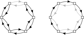
Figure 1: A bi-SCSS instance where all vertices are terminals. Left: Black edges show a solution which takes an undirected optimum twice. Right: The actual optimum solution is shown in black.

1.1 Our results

Bidirected inputs with planar solutions.

Our main theorem implies the existence of a PAS for bi-DSN${}_{\textsc{Planar}}$, where the parameter is the number $k$ of demands.

Theorem 1.1.

There is a $2^{O(k^{2})}n^{2^{O(1/{\varepsilon})}}$ time algorithm for bi-DSN${}_{\textsc{Planar}}$, that for any ${\varepsilon}>0$ computes a $(1+{\varepsilon})$-approximation.

This result begs the question of whether the considered special case is not too restrictive. Should it not be possible to obtain better runtimes and/or should it not be possible to even compute the optimum solution when parameterizing by $k$ for this very restricted problem? And could it not be that a similar result is true in more general settings, when for instance the input is bidirected but the optimum is not restricted to a planar graph? We prove that both questions can be answered in the negative.

First off, it is not hard to prove that a polynomial time approximation scheme (PTAS) is not possible for bi-DSN${}_{\textsc{Planar}}$, i.e., it is necessary to parameterize by $k$ in Theorem 1.1. This is implied by the following result, since (as mentioned before) a PTAS for bi-DSN${}_{\textsc{Planar}}$ would also imply a PTAS for bi-DST, i.e., the DST problem on bidirected input graphs.

Theorem 1.2.

The bi-DST problem (and by extension also the bi-DSN${}_{\textsc{Planar}}$ problem) is APX-hard.

One may wonder however, whether parameterizing by $k$ does not make the bi-DSN${}_{\textsc{Planar}}$ problem FPT, so that approximating the planar optimum as in Theorem 1.1 would in fact be unnecessary. Furthermore, even if it is necessary to approximate, one may ask whether the runtime given in Theorem 1.1 can be improved. In particular, note that the runtime we obtain in Theorem 1.1 is similar to that of a PTAS, i.e., the exponent of $n$ in the running time depends on ${\varepsilon}$. Ideally we would like an EPAS, which has a runtime of the form $f(k,{\varepsilon})\cdot n^{O(1)}$, i.e., we would like to treat ${\varepsilon}$ as a parameter as well. The following theorem shows that both approximation and runtime dependence on ${\varepsilon}$ are in fact necessary in Theorem 1.1.

Theorem 1.3.

The bi-DSN${}_{\textsc{Planar}}$ problem is W[1]-hard parameterized by $k$. Moreover, under ETH, for any computable functions $f(k)$ and $f(k,{\varepsilon})$, the bi-DSN${}_{\textsc{Planar}}$ problem

• has no $f(k)\cdot n^{o(\sqrt{k})}$ time algorithm to compute an optimum solution, i.e., a solution with cost at most that of the cheapest planar one, and

• has no $f(k,{\varepsilon})\cdot n^{o(\sqrt{k})}$ time algorithm to compute a solution with cost at most $(1+{\varepsilon})$ times that of the cheapest planar one, if ${\varepsilon}>0$ is part of the input.

It stands out that to compute optimum solutions, this theorem rules out runtimes for which the dependence of the exponent of $n$ is substantially better than $\sqrt{k}$, while for the general DSN problem, as mentioned above, the both necessary and sufficient dependence of the exponent is linear in $k$ [DBLP:journals/siamcomp/FeldmanR06, DBLP:conf/soda/ChitnisHM14]. Could it be that bi-DSN${}_{\textsc{Planar}}$ is just as hard as DSN when computing optimum solutions? The answer is no, as the next theorem shows.

Theorem 1.4.

There is a $2^{O(k^{3/2}\log k)}\cdot n^{O(\sqrt{k})}$ time algorithm to compute the optimum solution for bi-DSN${}_{\textsc{Planar}}$, i.e., a solution with cost at most that of the cheapest planar one.

This result is an example of the so-called “square-root phenomenon”: planarity often allows runtimes that improve the exponent by a square root factor in terms of the parameter when compared to the general case [planar-1, planar-2, planar-3, planar-4, planar-5, planar-6, planar-7, planar-8, new-planar]. Interestingly though, DBLP:conf/soda/ChitnisHM14 show that under ETH, no $f(k)\cdot n^{o(k)}$ time algorithm can compute the optimum solution to DSN${}_{\textsc{planar}}$. Thus assuming a bidirected input graph in Theorem 1.4 is necessary (under ETH) to obtain a factor of $O(\sqrt{k})$ in the exponent of $n$.

Bidirected inputs.

Since in contrast to bi-DSN${}_{\textsc{Planar}}$, the bi-DSN problem does not restrict the optimum solutions, one may wonder whether a parameterized approximation scheme as in Theorem 1.1 is possible for this more general case as well. We answer this in the negative by proving the following result, which implies that restricting the optima to planar graphs was necessary for Theorem 1.1.

Theorem 1.5.

Under Gap-ETH, there exists a constant $\alpha>1$ such that for any computable function $f(k)$ there is no $f(k)\cdot n^{O(1)}$ time algorithm that computes an $\alpha$-approximation for bi-DSN.

Also for the other obvious generalization of bi-DSN${}_{\textsc{Planar}}$, in which the input graph is unrestricted but we need to compute the planar optimum (i.e., the DSN${}_{\textsc{Planar}}$ problem), no parameterized approximation scheme exists. This follows from a recent result [Chitnis19-directed], which shows that no $(2-{\varepsilon})$-approximation can be computed for DSN${}_{\textsc{Planar}}$ in $f(k)\cdot n^{O(1)}$ time for any ${\varepsilon}>0$ and computable function $f$, under Gap-ETH.

What approximation factors can be obtained for bi-DSN when parameterizing by $k$, given the lower bound of Theorem 1.5 on one hand, and the before-mentioned result [DM18] that rules out a $k^{1/4-o(1)}$-approximation for DSN in time parameterized by $k$ on the other? It turns out that it is not too hard to obtain a constant approximation for bi-DSN, given the similarity of bidirected graphs to undirected graphs. In particular, relying on the fact that for the undirected version of DSN, i.e. the SF problem, there is a polynomial time $2$-approximation algorithm by steiner-forest, and an FPT algorithm based on DBLP:journals/networks/DreyfusW71, we obtain the following theorem, which is also in contrast to Theorem 1.2.

Theorem 1.6.

The bi-DSN problem admits a $4$-approximation in polynomial time, and a $2$-approximation in $2^{O(k)}\cdot n^{O(1)}$ time.

Even if Theorem 1.5 in particular shows that bi-DSN cannot be FPT under Gap-ETH, it does not give a strong lower bound on the runtime dependence in the exponent of $n$. However using the weaker ETH assumption we can obtain such a lower bound, as the next theorem shows. Interestingly, the obtained lower bound implies that when aiming for optimum solutions, the restriction to bidirected inputs does not make DSN easier than the general case, as also for bi-DSN the $n^{O(k)}$ time algorithm by DBLP:journals/siamcomp/FeldmanR06 is essentially best possible. This is in contrast to the bi-DSN${}_{\textsc{Planar}}$ problem where the square-root phenomenon takes effect as shown by Theorem 1.4.

Theorem 1.7.

The bi-DSN problem is W[1]-hard parameterized by $k$. Moreover, under ETH there is no $f(k)\cdot n^{o(k/\log k)}$ time algorithm for bi-DSN, for any computable function $f(k)$.

Strongly connected solutions.

Just like the more general DSN problem, the SCSS problem is W[1]-hard [DBLP:journals/siamdm/GuoNS11] parameterized by $k$, and is also hard to approximate as no polynomial time $O(\log^{2-{\varepsilon}}n)$-approximation is possible [approx-hardness], unless NP $\subseteq$ ZTIME$(n^{\text{polylog}(n)})$. However it is possible to exploit the structure of the optimum to SCSS to obtain a $2$-approximation algorithm parameterized by $k$, as observed by DBLP:conf/iwpec/ChitnisHK13. This is because any strongly connected graph is the union of two arborescences, and these form solutions to DST. The $2$-approximation follows, since DST is FPT by the classic result of DBLP:journals/networks/DreyfusW71. Thus in contrast to DSN, for SCSS it is possible to beat any approximation factor obtainable in polynomial time when parameterizing by $k$.

Theorem 1.8 ([DBLP:conf/iwpec/ChitnisHK13]).

The SCSS problem admits a $2$-approximation in $3^{k}\cdot n^{O(1)}$ time.

An obvious question now is whether the approximation ratio of this rather simple algorithm can be improved. Interestingly we are able to show that this is not the case. To the best of our knowledge, this is the first example of a problem with a tight parameterized approximation result with non-trivial approximation factor (in this case $2$), which also beats any approximation computable in polynomial time.

Theorem 1.9.

Under Gap-ETH, for any ${\varepsilon}>0$ and any computable function $f(k)$, there is no $f(k)\cdot n^{O(1)}$ time algorithm that computes a $(2-{\varepsilon})$-approximation for SCSS.

We remark that our reduction for Theorem 1.9 uses edge weights, which however can be polynomially bounded. As a consequence an instance can be further reduced in polynomial time by first scaling the edge weights to polynomially bounded integers, and then subdividing each edge $w$ times if its weight is $w$. This results in an equivalent unweighted instance, and thus the lower bound of Theorem 1.9 is also valid for unweighted instances of SCSS.

Bidirected inputs with strongly connected solutions.

In light of the above results for restricted cases of DSN, what can be said about restricted cases of SCSS? It is implicit in the work of DBLP:conf/soda/ChitnisHM14 that SCSS${}_{\textsc{Planar}}$, i.e., the problem of computing a solution of cost at most that of the cheapest strongly connected planar solution, can be solved in $2^{O(k\log k)}\cdot n^{O(\sqrt{k})}$ time, while under ETH no $f(k)\cdot n^{o(\sqrt{k})}$ time algorithm is possible. Hence SCSS${}_{\textsc{Planar}}$ is slightly easier than DSN${}_{\textsc{planar}}$ where the exponent of $n$ needs to be linear in $k$, as mentioned before. On the other hand, the bi-SCSS problem turns out to be a lot easier to solve than bi-DSN. This is implied by the next theorem, which stands in contrast to Theorem 1.5 and Theorem 1.7.

Theorem 1.10.

There is a $4^{k^{2}+O(k)}\cdot n^{O(1)}$ time algorithm for bi-SCSS, i.e., it is FPT for parameter $k$.

Could it be that bi-SCSS is even solvable in polynomial time? We prove that this is not the case, unless P = NP. To the best of our knowledge, the class of bidirected graphs is the first example where SCSS remains NP-hard but turns out to be FPT parameterized by $k$. Moreover, note that the above algorithm has an exponential runtime in $k^{2}$. We conjecture that a single exponential runtime should suffice, and we also obtain a lower bound result of this form.

Theorem 1.11.

The bi-SCSS problem is NP-hard. Moreover, under ETH there is no $2^{o(k)}\cdot n^{O(1)}$ time algorithm for bi-SCSS.

Remark.

For ease of notation, throughout this paper we chose to use the number of demands $k$ uniformly as the parameter. Alternatively one might also consider the smaller parameter $|R|$, where $R=\bigcup_{i=1}^{k}\{s_{i},t_{i}\}$ is the set of terminals (as also done in [DBLP:conf/stacs/EibenKPS19]). Note for instance that in case of the SCSS problem, $k=|R|$, while for DSN, $k$ can be as large as $\Theta(|R|^{2})$. However we always have $k\geq|R|/2$, since the demands can form a matching in the worst case. It is interesting to note that all our algorithms for DSN have the same running time for parameter $|R|$ as for parameter $k$. That is, we may set $k=|R|$ in Theorem 1.1, Theorem 1.4, and Theorem 1.6.

	algorithms			lower bounds
problem	approx.	runtime	ref.	approx.	runtime	ref.
DSN	–	$n^{O(k)}$	[DBLP:journals/siamcomp/FeldmanR06]	–	$f(k)\cdot n^{o(k)}$	[DBLP:conf/stacs/EibenKPS19, DBLP:journals/siamdm/GuoNS11]
DSN	$O(k^{\frac{1}{2}+{\varepsilon}})$	$n^{O(1)}$	[DBLP:journals/talg/ChekuriEGS11]	$k^{\frac{1}{4}-o(1)}$	$f(k)\cdot n^{O(1)}$	[DM18]
DSN${}_{\textsc{TW: }\omega}$	–	$2^{O(k\omega\log\omega)}\cdot n^{O(\omega)}$	[DBLP:conf/icalp/FeldmannM16]	–	$f(k,\omega)\cdot n^{o(\omega)}$	[DBLP:conf/icalp/FeldmannM16]
bi-DSN${}_{\textsc{Planar}}$	–	$2^{O(k^{3/2}\log k)}\cdot n^{O(\sqrt{k})}$	Thm 1.4	–	$f(k)\cdot n^{o(\sqrt{k})}$	Thm 1.3
bi-DSN${}_{\textsc{Planar}}$	$1+{\varepsilon}$	$2^{O(k^{2})}n^{2^{O(1/{\varepsilon})}}$	Thm 1.1	$1+{\varepsilon}$	$f(\varepsilon,k)\cdot n^{o(\sqrt{k})}$	Thm 1.3
DSN${}_{\textsc{Planar}}$	–	$n^{O(k)}$	[DBLP:conf/stacs/EibenKPS19, DBLP:journals/siamcomp/FeldmanR06]	–	$f(k)\cdot n^{o(k)}$	[DBLP:conf/soda/ChitnisHM14]
DSN${}_{\textsc{Planar}}$	$\alpha\geq 2$	(open)		$(2-{\varepsilon})$	$f(k)\cdot n^{O(1)}$	[Chitnis19-directed]
bi-DSN	–	$n^{O(k)}$	[DBLP:journals/siamcomp/FeldmanR06]	–	$f(k)\cdot n^{o(k/\log k)}$	Thm 1.7
bi-DSN	2	$2^{O(k)}\cdot n^{O(1)}$	Thm 1.6	$\alpha\in\Theta(1)$	$f(k)\cdot n^{O(1)}$	Thm 1.5
bi-DSN	$4$	$n^{O(1)}$	Thm 1.6	$\alpha\in\Theta(1)$	$n^{O(1)}$	Thm 1.2
SCSS	–	$n^{O(k)}$	[DBLP:journals/siamcomp/FeldmanR06]	–	$f(k)\cdot n^{o(k/\log k)}$	[DBLP:journals/siamdm/GuoNS11, DBLP:conf/soda/ChitnisHM14]
SCSS	$2$	$3^{k}\cdot n^{O(1)}$	[DBLP:conf/iwpec/ChitnisHK13]	$2-{\varepsilon}$	$f(k)\cdot n^{O(1)}$	Thm 1.9
SCSS${}_{\textsc{Planar}}$	–	$2^{O(k\log k)}\cdot n^{O(\sqrt{k})}$	[DBLP:conf/soda/ChitnisHM14]	–	$f(k)\cdot n^{o(\sqrt{k})}$	[DBLP:conf/soda/ChitnisHM14]
bi-SCSS	–	$4^{k^{2}+O(k)}\cdot n^{O(1)}$	Thm 1.10	–	$2^{o(k)}\cdot n^{O(1)}$	Thm 1.11

Table 1: Summary of achievable runtimes for DSN and SCSS when parameterizing by $k$. A dash (–) refers to computing optimum solutions. Some of the previous results are implicit and in the papers are rather stated for the case when the input graphs are restricted to the same class as the optimum solutions.

1.2 Our techniques

It is already apparent from the above exposition of our results, that understanding the structure of the optimum solution is a powerful tool when studying DSN and its related problems (cf. Table 1). This is also apparent when reading the literature on these problems, and we draw some of our inspiration from these known results, as described below.

Approximation scheme for bi-DSN${}_{\textsc{Planar}}$.

We generalize the insights on the structure of optimum solutions to the classical Steiner Tree (ST) problem for our main result in Theorem 1.1. For the ST problem, an undirected edge-weighted graph is given together with a terminal set $R$, and the task is to compute the cheapest tree connecting all $k$ terminals. For this problem only polynomial-time $2$-approximations were known [GP68, V01], until it was taken into account [KZ97, PS00, zelikovsky_1993_11_over_6_apx, RZ05] that any optimum Steiner tree can be decomposed into so-called full components, i.e., subtrees for which exactly the leaves are terminals. If a full component contains only a small subset of size $k^{\prime}$ of the terminals, it is the solution to an ST instance, for which the optimum can be computed efficiently in time $3^{k^{\prime}}\cdot n^{O(1)}$ using the algorithm of DBLP:journals/networks/DreyfusW71. A fundamental observation proved by borchers-du is that for any $k^{\prime}$ there exists a solution to ST of cost at most $1+\frac{1}{\lfloor\log_{2}k^{\prime}\rfloor}$ times the optimum, in which every full component contains at most $k^{\prime}$ terminals. Thus setting $k^{\prime}=2^{1/{\varepsilon}}$ for some constant ${\varepsilon}>0$, all full-components with at most $2^{1/{\varepsilon}}$ terminals can be computed in polynomial time, and among them exists a collection forming a $(1+{\varepsilon})$-approximation. The key to obtain approximation ratios smaller than $2$ for ST is to cleverly select a good subset of all computed full-components. This is for instance done in [DBLP:journals/jacm/ByrkaGRS13] via an iterative rounding procedure, resulting in an approximation ratio of $\ln(4)+{\varepsilon}<1.39$, which currently is the best one known.

Our main technical contribution is to generalize the borchers-du Theorem to bi-DSN${}_{\textsc{Planar}}$. In particular, to obtain our approximation scheme of Theorem 1.1, we employ a similar approach by decomposing a bi-DSN${}_{\textsc{Planar}}$ solution into sub-instances, each containing a small number of terminals. As bi-DSN${}_{\textsc{Planar}}$ is W[1]-hard by Theorem 1.3, we cannot hope to compute optimum solutions to each sub-instance as efficiently as for ST. However, we provide an XP-algorithm with runtime $2^{O(k^{3/2}\log k)}\cdot n^{O(\sqrt{k})}$ for bi-DSN${}_{\textsc{Planar}}$ in Theorem 1.4. Thus if every sub-instance contains at most $2^{1/{\varepsilon}}$ terminals, each can be solved in $n^{2^{O(1/{\varepsilon})}}$ time, and this accounts for the “non-efficient” runtime of our approximation scheme. Since we allow runtimes parameterized by $k$, we can then search for a good subset of precomputed small optimum solutions to obtain a solution to the given demand set ${\mathcal{D}}$. For the latter solution to be a $(1+{\varepsilon})$-approximation however, we need to generalize the borchers-du Theorem for ST to bi-DSN${}_{\textsc{Planar}}$ (see Theorem 4.1 for the formal statement). This constitutes the bulk of the work to prove Theorem 1.1.

Exact algorithms for bi-DSN${}_{\textsc{Planar}}$ and bi-SCSS.

Also from a parameterized point of view, understanding the structure of the optimum solution to DSN has lead to useful insights in the past. We will leverage one such recent result by DBLP:conf/icalp/FeldmannM16, where the above mentioned standard special case of restricting the patterns of the demands in ${\mathcal{D}}$ is studied in depth. The result is a complete dichotomy over which classes of restricted patterns define special cases of DSN that are FPT and which are W[1]-hard for parameter $k$. The high-level idea is that whenever the demand patterns imply optimum solutions of constant treewidth, there is an FPT algorithm computing such an optimum. In contrast, the problem is W[1]-hard whenever the demand patterns imply the existence of optimum solutions of arbitrarily large treewidth. The FPT algorithm from [DBLP:conf/icalp/FeldmannM16] lies at the heart of all our positive results, and therefore shows that the techniques developed in [DBLP:conf/icalp/FeldmannM16] to optimally solve special cases of DSN can be extended to find (near-)optimum solutions for other W[1]-hard special cases as well. It is important to note that the algorithm of [DBLP:conf/icalp/FeldmannM16] can also be used to compute the cheapest solution of treewidth at most $\omega$, even if there is an even better solution of treewidth larger than $\omega$ (which might be hard to compute). Formally, the result leveraged in this paper is the following.

Theorem 1.12 (implicit in Theorem 5 of [DBLP:conf/icalp/FeldmannM16]).

If ${\mathcal{K}}$ is the class of graphs with treewidth at most $\omega$, then the DSN${}_{\mathcal{K}}$ problem can be solved in $2^{O(k\omega\log\omega)}\cdot n^{O(\omega)}$ time.

We exploit the algorithm given by Theorem 1.12 to prove our algorithmic results of Theorem 1.4 and Theorem 1.10. In particular, we prove that any bi-DSN${}_{\textsc{Planar}}$ solution has treewidth $O(\sqrt{k})$, from which Theorem 1.4 follows immediately. For bi-SCSS however, we give an example of an optimum solution of treewidth $\Omega(k)$. Hence we cannot exploit the algorithm of Theorem 1.12 directly to obtain Theorem 1.10. In fact on general input graphs, a treewidth of $\Omega(k)$ would imply that the problem is W[1]-hard by the hardness results in [DBLP:conf/icalp/FeldmannM16] (which was indeed originally shown by DBLP:journals/siamdm/GuoNS11). As this stands in stark contrast to Theorem 1.10, it is particularly interesting that the SCSS problem on bidirected input graphs is FPT. We prove this result by decomposing an optimum solution to bi-SCSS into sub-instances of bi-SCSS${}_{\mathcal{K}}$, where ${\mathcal{K}}$ is a class of directed graphs of treewidth $1$ (so-called poly-trees). For each such sub-instance we can compute a solution in $2^{O(k)}\cdot n^{O(1)}$ time by using Theorem 1.12 (for $\omega=1$), and then combine them into an optimum solution to bi-SCSS.

W[1]-hardness and runtime lower bounds.

Our hardness proofs for bi-DSN are based on reductions from the Grid Tiling problem [pc-book]. This problem is particularly well-suited to prove hardness for problems on planar graphs, due to its grid-like structure. We first develop a specific gadget that can be exploited to show hardness for bidirected graphs. This gadget however is not planar. We only exploit the structure of Grid Tiling to show that the optimum solution is planar for Theorem 1.3. For Theorem 1.7 we modify this reduction to obtain a stronger runtime lower bound, but in the process we lose the property that the optimum is planar.

Parameterized inapproximability.

Our hardness result for SCSS is proved by combining a variant of a known reduction by DBLP:journals/siamdm/GuoNS11 with a recent parameterized hardness of approximation result for Densest $k$-Subgraph [param-inapprox]. Our inapproximability result for bi-DSN is shown by combining our W[1]-hardness reduction with the same hardness of approximation result of Densest $k$-Subgraph.

1.3 Approximate kernelization

A topic closely related to parameterized algorithms is kernelization, which concerns efficient pre-processing algorithms. As formalized by lokshtanov2017lossy, an $\alpha$-approximate kernel for an optimization problem consists of a reduction and a lifting algorithm, both running in polynomial time. The reduction algorithm takes an instance $I$ with parameter $k$ and computes a new instance $I^{\prime}$ and parameter $k^{\prime}$, such that the size $|I^{\prime}|+k^{\prime}$ of the new instance is bounded by some function $f(k)$ of the input parameter. This new instance $I^{\prime}$ is also called a kernel of $I$. The lifting algorithm takes as input any $\beta$-approximation for the kernel $I^{\prime}$ and computes an $\alpha\beta$-approximate solution for $I$.

It has long been known that a problem is FPT if and only if it admits an exact kernel, i.e., a $1$-approximate kernel. lokshtanov2017lossy prove that this is also the case in general: a problem has a parameterized $\alpha$-approximation algorithm if and only if it admits an $\alpha$-approximate kernel. Note that the size of the kernel might in general be very large, even if it is bounded in the input parameter. Therefore a well-studied interesting question is whether a polynomial-sized kernel exists, which can be taken as evidence that a problem admits a very efficient pre-processing algorithm. If a problem admits a polynomial-sized $(1+{\varepsilon})$-approximate kernel for every ${\varepsilon}>0$, then we say that it admits a polynomial-sized approximate kernelization scheme (PSAKS).

The ST problem is known to be FPT [DBLP:journals/networks/DreyfusW71], while not admitting any polynomial-sized exact kernel [dom] for parameter $k$, unless NP $\subseteq$ coNP/Poly. However, as noted by lokshtanov2017lossy, the borchers-du Theorem implies the existence of a PSAKS for the ST problem. As a consequence of our generalization of the borchers-du Theorem we also obtain a PSAKS for bi-DSN${}_{\textsc{Planar}}$ (see Section 4 for a formal statement). This is despite the fact that this problem does not admit any exact kernel for parameter $k$ according to Theorem 1.3. Furthermore, we observe that the same kernel is in fact a polynomial-sized $(2+{\varepsilon})$-approximate kernel for the bi-DSN problem. This nicely complements the existence of a parameterized $2$-approximation algorithm according to Theorem 1.6.

1.4 Related work

The ST problem is one of the 21 NP-hard problems listed in the seminal paper of MR51:14644. DBLP:journals/networks/DreyfusW71 showed that the problem is solvable in time $3^{k}\cdot n^{O(1)}$, which was later improved [fuchs2007dynamic] to $(2+{\varepsilon})^{k}\cdot n^{O(1)}$ for any constant ${\varepsilon}>0$. For values $k>2\log n\log^{3}\log n$ an even faster algorithm exists [vygen2011faster]. For unweighted graphs an algorithm with runtime $2^{k}\cdot n^{O(1)}$ can be obtained [BjorklundHKK07, DBLP:journals/algorithmica/Nederlof13]. An early LP-based $2$-approximation algorithm for ST uses the so-called bidirected cut relaxation (BCR) [wong1984dual, E67, feldmann2016equivalence], which formulates the problem by bidirecting the undirected input graph. Thus bidirected instances have implicitly been used even for the classical ST problem since the 1960s. For ST and SF there are PTASes on planar and bounded genus graphs [bateni2011approximation, eisenstat2012efficient].

A recent result [DBLP:conf/stacs/EibenKPS19] investigates the complexity of DSN with respect to the stronger parameter $|R|$ (instead of the number of demands $k$; see remark above). It is shown that for bounded genus graphs the DSN problem can be solved in $f(|R|)\cdot n^{O(|R|)}$ time, while in general no $f(|R|)\cdot n^{o(|R|^{2}/\log|R|)}$ time algorithm exists, under ETH. The DST problem has an $O(k^{\varepsilon})$-approximation in polynomial time [DBLP:journals/jal/CharikarCCDGGL99], and an $O(\log^{2}k/\log\log k)$-approximation in quasi-polynomial time [DBLP:conf/stoc/0001LL19]. Moreover, no better approximation is possible in quasi-polynomial time [DBLP:conf/stoc/0001LL19]. A long standing open problem is whether a polynomial-time algorithm with poly-logarithmic approximation guarantee exists for DST. The SCSS problem has also been studied in the special case when $R=V$. This case is commonly known as Minimum Strongly Connected Spanning Subgraph, and the best approximation factor known is $2$, which is also given by computing two spanning arborescences [frederickson1981approximation], and for $R=V$ can be done in polynomial time. For the unweighted case however, a $3/2$-approximation is obtainable [vetta2001approximating], which is contrast to unweighted SCSS, where the lower bound of Theorem 1.9 is also valid.

Bidirected input graphs have been studied in the context of radio and ad-hoc wireless networks [chen1989strongly, ramanathan2000topology, wang2008approximate, lam2015dual]. In the Power Assignment problem, nodes of a given bidirected network need to be activated in order to induce a network satisfying some connectivity condition. For instance in [chen1989strongly], the problem of finding a strongly connected network is considered, but also other settings such as $2$-(vertex/edge)-connectivity [wang2008approximate] or $k$-(vertex/edge)-connectivity [lam2015dual] have been studied.

1.5 Organization of the paper

We give some preliminaries and basic observations on the structure of optimum solutions to bi-DSN in bidirected input graphs in Section 2. These are used throughout Section 4, where we present our approximation scheme for bi-DSN${}_{\textsc{Planar}}$ of Theorem 1.1, and LABEL:sec:alg-opt, where we show how to compute optimum solutions to bi-DSN${}_{\textsc{Planar}}$ for Theorem 1.4 and bi-SCSS for Theorem 1.10. Before presenting our main result of Section 4 however, we first need to develop the approximation algorithms for bi-DSN of Theorem 1.6, which we do in Section 3 together with the hardness result for bi-DSN${}_{\textsc{Planar}}$ of Theorem 1.2. The inapproximability results for bi-DSN of Theorem 1.5 and SCSS of Theorem 1.9 are given in LABEL:sec:inapprox, and the remaining runtime lower bounds for bi-DSN${}_{\textsc{Planar}}$ of Theorem 1.3, bi-DSN of Theorem 1.7, and bi-SCSS of Theorem 1.11 can be found in LABEL:sec:lb. In LABEL:app:dsn we present the reduction that was used later by DM18 to prove the $k^{1/4-o(1)}$-approximation hardness for DSN. Finally, in LABEL:sec:questions we list some open questions.

2 Structural properties of optimum solutions to bi-DSN

In this section we give some definitions relevant to directed and bidirected graphs, and some fundamental observations on solutions to bi-DSN that we will use throughout the paper.

Due to the similarity of bidirected graphs to undirected graphs, we will often exploit the structure of the underlying undirected graph of a given bidirected graph. More generally, for any directed graph $G$ we denote the underlying undirected graph by $\overline{G}$. A poly-graph is obtained by directing the edges of an undirected graph, and analogously we obtain poly-cycles, poly-paths, and poly-trees. A strongly connected poly-cycle is a directed cycle, and a poly-tree for which all vertices can reach (or are reachable from) a designated root vertex $r$ is called an out-arborescence (or in-arborescence). Note that for any edge $uv$ of a poly-graph, the reverse edge $vu$ does not exist, and so a poly-graph is in a sense the opposite of a bidirected graph. In between poly-graphs and bidirected graphs are general directed graphs.

2.1 Cycles of optimum solutions in bidirected graphs

We need the following observation, which has far reaching consequences for bi-DSN algorithms. An optimum bi-DSN solution may contain poly-cycles, which are not directed cycles: consider for instance a bidirected graph for which the underlying undirected graph is a cycle on four vertices and every edge has unit weight. If the vertices are numbered $1,2,3,4$ along the cycle and the demands are $\{(1,2),(1,4),(3,2),(3,4)\}$, then it is not hard to see that an optimum solution is given by the poly-cycle with edges corresponding to the demands, i.e., the edge set $\{(1,2),(1,4),(3,2),(3,4)\}$. As the following lemma shows however, any such poly-cycle can be replaced by a directed cycle.

Lemma .

Let $O$ be a poly-cycle of a subgraph $N\subseteq G$ in a bidirected graph $G$. Replacing $O$ with a directed cycle on $V(O)$ in $N$ results in a subgraph $M$ of $G$ with cost at most that of $N$, such that a $u\to v$ path exists in $M$ for every vertex pair $u,v$ for which $N$ contained a $u\to v$ path.

Proof.

Removing all edges of $O$ in $N$ and replacing them with a directed cycle cannot increase the cost, as $G$ is bidirected (the cost may decrease if an edge $uv$ of $O$ is replaced by an edge $vu$, which is already contained in $N$). Any $u\to v$ path that leads through $O$ in $N$ can be rerouted through the strongly connected directed cycle in $M$. ∎

From this we can deduce the following useful observation, which we will exploit for all of our algorithms. The intuitive meaning of it is that any poly-cycle of an optimum bi-DSN solution splits the solution into parts of which each contains at least one terminal.

Lemma .

Let $N\subseteq G$ be an optimum bi-DSN solution in a bidirected graph $G$, such that $N$ contains a poly-cycle $O\subseteq N$. Every edge of $N$ that is incident to two vertices of $O$ is also part of $O$. Moreover, every connected component of the graph resulting from removing $V(O)$ from $N$ contains at least one terminal.

Proof.

By Section 2.1 we may exchange $O$ with a directed cycle $O^{\prime}$ without increasing the cost and maintaining all connections for the demands given by the bi-DSN instance. Since $N$ has minimum cost, this means that the resulting network $N^{\prime}$ is also an optimum solution. Assume that $N$ contained some edge $e$ incident to two vertices of $O$ but $e\notin E(O)$. The edge $e$ cannot be a reverse edge of some edge $f$ of $O$, as we could replace $O$ with a cycle directed in the same direction as $e$. This would decrease the cost as $N^{\prime}$ only contains $e$, while $N$ contains both $e$ and $f$. We are left with the case that $e$ is a chord of $O$, i.e., it connects two non-adjacent vertices of $O$. However in this case, the endpoints of $e$ are strongly connected through $O^{\prime}$ in $N^{\prime}$ even after removing $e$. Thus we would be able to safely remove $e$ and decrease the cost of $N^{\prime}$.

Now assume that some connected component $C$ of the graph obtained from $N$ by removing $V(O)$ contains no terminal. Note that $C$ also exists in the graph obtained from $N^{\prime}$ by removing $O^{\prime}$ and its vertices. As $C$ contains no terminals, any $s\to t$ path in $N^{\prime}$ for a demand $(s,t)$ that contains a vertex of $C$ must contain a $u\to v$ subpath for some vertices $u,v\in V(O^{\prime})$ with internal vertices from $C$. However the vertices $u,v$ are strongly connected through $O^{\prime}$ and hence the $u\to v$ subpath can be rerouted via $O^{\prime}$. This means we may safely remove $C$ from $N^{\prime}$ without loosing any connections for the required demands. However this contradicts the optimality of $N^{\prime}$, and in turn also our assumption that $N$ is an optimum solution. ∎

2.2 Reducing the vertex degrees

For our proofs, it will be convenient to assume that the degrees of the vertices in some given graph are bounded. More specifically, consider a (possibly planar) graph $N$ connecting a terminal set $R$ according to some set of demands. We use the standard procedure below, which assures that every terminal has only one neighbour in $N$, and every Steiner vertex of $N$, i.e. every non-terminal in $V(N)\setminus R$, has exactly three neighbours in $N$.

We execute the following steps on $N$ in the given order. It is easy to see that these operations preserve planarity (if $N$ is planar), the cost of $N$, and the connectivity according to the demands.

1. For every terminal $t\in R$ that has more than one neighbour in $N$, we introduce a new Steiner vertex $v$ and add the edges $vt$ and $tv$ with cost $0$ each. Thereafter every neighbour $w$ of $t$ different from $v$ is made a neighbour of $v$ instead. That is, the edges $wt$ and $tw$ are replaced by the edges $wv$ and $vw$ of the same cost. After this, every terminal in $N$ has one neighbour only.

2. Then for every Steiner vertex $v$ with more than $3$ neighbours in $N$, we split $v$ into two vertices as follows. In case $N$ is planar we first fix a drawing of $N$. Then we introduce a new Steiner vertex $u$ and edges $uv$ and $vu$ with cost $0$ each. As the new vertex only has one neighbour, we may draw $u$ in an arbitrary face of $N$ that is incident to $v$. Let $F$ be this face containing $u$, and let $w_{1}$ and $w_{2}$ be the two neighbours of $v$ incident to $F$ that are different from $u$. For each $j\in\{1,2\}$, we replace the edges $vw_{j}$ and $w_{j}v$ with edges $uw_{j}$ and $w_{j}u$, respectively. We maintain the edge costs in each of these replacement steps. Note that $N$ remains planar under this operation. In case $N$ is not planar, we proceed in the same way but simply pick arbitrary neighbours $w_{1},w_{2}$ of $v$ that are different from $u$. After repeating this for every Steiner vertex with more than $3$ neighbours, all Steiner vertices of $N$ have at most three neighbours.

3. Next we consider each Steiner vertex $v$ that has exactly two neighbours $u$ and $w$. If $N$ contains the path $uvw$, we add an edge $uw$ with the same cost as the path. Similarly, if $N$ has a $wvu$ path, we introduce the edge $wu$ with the same cost. We then remove the vertex $v$. After this all Steiner vertices of $N$ have exactly three neighbours.

3 Hardness and algorithms for bi-DSN via undirected graphs

In this section we present two results for problems on bidirected graphs that follow from corresponding results on undirected graphs. We first prove Theorem 1.2, which we restate below. In particular, it implies that bi-DSN${}_{\textsc{Planar}}$ has no PTAS, unless P=NP.

See 1.2

Proof.

Given a Steiner Tree (ST) instance on an undirected graph $\overline{G}$, we simply bidirect each edge to obtain the bidirected graph $G$. We then choose any of the terminals in $G$ as the root to get an instance of bi-DST. It is easy to see that any solution to ST in $\overline{G}$ corresponds to a solution to bi-DST in $G$ of the same cost, and vice versa. As the ST problem is APX-hard [chlebik2002approximation], the hardness carries over to bi-DST. ∎

Note that as the definition of the ST problem does not restrict the feasible solutions to trees, this hardness result does not restrict the approximate solutions to bi-DST to arborescences either. That is, it is also hard to compute an approximation $N$ to the optimum bi-DSN${}_{\textsc{Planar}}$ solution, even if we allow $N$ to be a non-planar graph.

Next we turn to the positive result of Theorem 1.6, which we also restate below. Note that this theorem is in contrast to Theorem 1.2 and Theorem 1.5.

See 1.6

Proof.

Given a bidirected graph $G$ and a demand set ${\mathcal{D}}=\{(s_{i},t_{i})\mid 1\leq i\leq k\}$ of an instance to bi-DSN, we reduce it to an instance of the Steiner Forest (SF) problem in the underlying undirected graph $\overline{G}$ with the corresponding unordered demand set $\overline{{\mathcal{D}}}=\{\{s_{i},t_{i}\}\mid(s_{i},t_{i})\in{\mathcal{D}}\}$. The returned bi-DSN solution is the network $N\subseteq G$ that contains both edges $uv$ and $vu$ for any undirected edge between $u$ and $v$ of the SF solution computed for $\overline{G}$. Thus the cost of $N$ is at most twice the cost of the SF solution. At the same time, the optimum SF solution in $\overline{G}$ has cost at most that of the optimum bi-DSN solution in $G$, since taking the underlying undirected graph of the latter is an SF solution in $\overline{G}$.

The first part of theorem now follows by using the polynomial time $2$-approximation algorithm steiner-forest for the SF problem. We now show how to solve the SF problem in $2^{O(k)}\cdot n^{O(1)}$ time using the FPT algorithm of DBLP:journals/networks/DreyfusW71 for the ST problem which runs in $3^{p}\cdot n^{O(1)}$ time where $p$ is number of terminals. However, as observed in [DBLP:conf/icalp/FeldmannM16], it can also easily be used for SF as well: the optimum solution to SF is a forest and therefore the terminal set can be partitioned so that each part is a tree in the optimum. We now use dynamic programming: for each $X\subseteq[k]$ let $\text{OPT}[X]$ denote the minimum cost solution for the instance of SF with the terminal pairs $\overline{{\mathcal{D}}}_{X}:=\{\{s_{i},t_{i}\}\mid i\in X\}$. We define $\text{OPT}[\emptyset]=0$. Then, we have the following recurrence

$$\text{OPT}[X]=\min_{Y\subseteq X,Y\neq\emptyset}\Big{\{}\text{DF}[Y]+\text{OPT}[X\setminus Y]\Big{\}}$$

where $\text{DF}[Y]$ is the cost obtained by running the Dreyfus-Wagner algorithm on the instance of ST whose terminal set is $Y$. The correctness of the recurrence follows since the forest which forms the optimal solution of the instance of SF with terminal pairs $\overline{{\mathcal{D}}}_{X}$ must contain some non-empty subset of the terminal pairs in one of its trees. The final answer that we output is $\text{OPT}\big{[}[k]\big{]}$. Since the running time of the Dreyfus-Wagner algorithm is $3^{p}\cdot n^{O(1)}$, the running time of the dynamic program is ∑_i=1^k (ki)⋅( ∑_j=1^i 3^2j⋅n^O(1)) ≤9⋅n^O(1)⋅(∑_i=1^k (ki)⋅9^i ) = 2^O(k)⋅n^O(1)∎

In Section 4 we will prove that a PSAKS exists for the bi-DSN${}_{\textsc{Planar}}$ problem. One ingredient for this will be the existence of a polynomial time algorithm that gives a good estimate of the cost of a planar optimum solution. The $4$-approximation algorithm of Theorem 1.6 provides a good lower bound on the cost of the overall optimum, and thus also for the planar optimum. However, a priori this does not provide a good upper bound, since the planar optimum might cost a lot more than the overall optimum, and thus than the approximation. Note though that both algorithms of Theorem 1.6 compute planar solutions, and hence they also upper bound the optimum planar solution. In particular, the existence of a planar $2$-approximation of the optimum solution to bi-DSN implies that the planar optimum cannot cost more than twice the overall optimum, as summarized below.

Corollary .

For any bi-DSN instance with optimum solution $N$, there exists a planar solution $N^{\prime}$ such that $\operatorname{cost}(N^{\prime})\leq 2\operatorname{cost}(N)$.

4 An approximation scheme for bi-DSN${}_{\textsc{Planar}}$

In this section we prove Theorem 1.1, which is restated below. Note that since we have $k$ demand pairs, it follows that the number $|R|$ of terminals is at most $2k$, where $R=\bigcup_{i=1}^{k}\{s_{i},t_{i}\}$. Henceforth in this section, we use the upper bound $2k$ on the number of terminals $|R|$ for ease of presentation (when instead we could replace $k$ by $|R|$ in the running time of Theorem 1.1).

See 1.1

The bulk of the proof is captured by the following result, which generalizes the corresponding theorem by borchers-du for the ST problem, and which is our main technical contribution. In order to facilitate the definition of a sub-instance to DSN, we encode the demands of a DSN instance using a pattern graph $H$, as also done in [DBLP:conf/icalp/FeldmannM16]: the vertex set of $H$ is the terminal set $R$, and $H$ contains the directed edge $st$ if and only if $(s,t)$ is a demand. Hence the DSN problem asks for a minimum cost network $N\subseteq G$ having an $s\to t$ path for each edge $st$ of $H$. Here $\operatorname{cost}(N)$ denotes the cost of a graph (solution) $N$, i.e., the sum of its edge weights.

Theorem 4.1.

Let $G$ be a bidirected graph, and $H$ a pattern graph on $R\subseteq V(G)$. Let $N\subseteq G$ be the cheapest planar solution to pattern $H$. For any ${\varepsilon}>0$, there exists a set of patterns ${\mathcal{H}}$ such that

1. $V(H^{\prime})\subseteq R$ with $|V(H^{\prime})|\leq 2^{1+1/{\varepsilon}}$ for each $H^{\prime}\in{\mathcal{H}}$,

2. given any feasible solutions $N_{H^{\prime}}\subseteq G$ for all $H^{\prime}\in{\mathcal{H}}$, the union $\bigcup_{H^{\prime}\in{\mathcal{H}}}N_{H^{\prime}}$ of the these solutions forms a feasible solution to $H$, and

3. there exist feasible planar solutions $N^{*}_{H^{\prime}}\subseteq G$ for all $H^{\prime}\in{\mathcal{H}}$ such that
   $\sum_{H^{\prime}\in{\mathcal{H}}}\operatorname{cost}(N^{*}_{H^{\prime}})\leq(1+{\varepsilon})\cdot\operatorname{cost}(N)$.

Note that the pattern graphs $H^{\prime}$ of the set ${\mathcal{H}}$ in this theorem do not have to be subgraphs of the given pattern $H$. In fact, as the proof of Theorem 4.1 below shows, in general they are not. Before we give the proof, we describe the consequences of this theorem.

Consequences of Theorem 4.1.

Our approximation scheme of Theorem 1.1 will compute optimum planar solutions to all patterns with at most $2^{1+1/{\varepsilon}}$ terminals using the XP algorithm of Theorem 1.4, and then essentially find the set ${\mathcal{H}}$ of Theorem 4.1 via a dynamic program. This is captured in the following proof.

Proof of Theorem 1.1..

The first step of the algorithm is to consider every possible pattern graph on at most $g({\varepsilon})=2^{1+1/{\varepsilon}}$ terminals from $R$. For each such pattern $H^{\prime}$ the algorithm computes an optimum bi-DSN${}_{\textsc{Planar}}$ solution $N_{H^{\prime}}$ (if any) using the algorithm of Theorem 1.4. Since any considered pattern graph has at most $2{g({\varepsilon})\choose 2}<g({\varepsilon})^{2}$ edges, and (regardless of the input pattern $H$) there is a total of $2{2k\choose 2}<4k^{2}$ possible demands between the at most $2k$ terminals of $R$, the total number of considered pattern graphs is less than $\sum_{i=0}^{g({\varepsilon})^{2}}{4k^{2}\choose i}=k^{2^{O(1/{\varepsilon})}}$. An optimum planar solution (if it exists) to each of these patterns is computed in $2^{g({\varepsilon})^{3/2}\log g({\varepsilon})}\cdot n^{O(\sqrt{g({\varepsilon})})}=n^{2^{O(1/{\varepsilon})}}$ time via Theorem 1.4. Hence up to now the algorithm takes $n^{2^{O(1/{\varepsilon})}}$ time, as $k\in O(n^{2})$.

The next step is to use a dynamic program to compute a solution to the input pattern $H$ by putting together these pre-computed planar solutions. More concretely, let $N_{1},\ldots,N_{p}$ be all the solutions computed in the first step (given in any arbitrary order). For any subset ${\mathcal{N}}$ of these planar graphs, in the following we denote by $\operatorname{cost}({\mathcal{N}}):=\sum_{N\in{\mathcal{N}}}\operatorname{cost}(N)$ their total cost and by $\bigcup{\mathcal{N}}:=\bigcup_{N\in{\mathcal{N}}}N$ their union. For $1\leq i\leq p$ and any pattern graph $H^{\prime}$, we define σ(H’,i)=min{cost(N) — N⊆{N_1, …,N_i} and ⋃N feasible for H’} to be the minimum total cost of a subset of the first $i$ planar graphs $N_{1},\ldots,N_{i}$ that forms a feasible solution to $H^{\prime}$. Note that the total cost of a set ${\mathcal{N}}$ counts edges appearing in more than one graphs of ${\mathcal{N}}$ several times. If no feasible solution to $H^{\prime}$ can be obtained from any subset of $N_{1},\ldots,N_{i}$, then we define $\sigma(H^{\prime},i)$ to be $\infty$.

Let ${\mathcal{H}}$ be the set of patterns given by Theorem 4.1 for the optimum planar solution $N$ to $H$, and let $N^{*}_{H^{\prime}}$ be the planar solution to each $H^{\prime}\in{\mathcal{H}}$ given by the theorem. The existence of $N^{*}_{H^{\prime}}$ implies that for each $H^{\prime}\in{\mathcal{H}}$ there is also a feasible planar solution $N_{H^{\prime}}$ among $N_{1},\ldots,N_{p}$, and by Theorem 4.1 their union $\bigcup_{H^{\prime}\in{\mathcal{H}}}N_{H^{\prime}}$ is a feasible solution to $H$. Thus σ(H,p)≤∑_H’∈H cost(N_H’) ≤∑_H’∈H cost(N^*_H’) = (1+ε)cost(N), where the second inequality follows since each computed planar solution $N_{i}$ (and thus each $N_{H^{\prime}}$ where $H^{\prime}\in{\mathcal{H}}$) is an optimum solution due to Theorem 1.4. We conclude that $\sigma(H,p)$ is the value of a $(1+{\varepsilon})$-approximation to the optimum bi-DSN${}_{\textsc{Planar}}$ solution.

To recursively compute $\sigma(H^{\prime},i)$ for any pattern graph $H^{\prime}$ on $R$ and any $1\leq i\leq p$, we keep track of the subset ${\mathcal{N}}^{i}_{H^{\prime}}\subseteq\{N_{1},\ldots,N_{i}\}$ of planar graphs that obtain the cost stored by the following dynamic program in $\sigma(H^{\prime},i)$. For $i=1$ we just check whether $N_{1}$ is a feasible solution to $H^{\prime}$. If so, we set $\sigma(H^{\prime},1)=\operatorname{cost}(N_{1})$ and ${\mathcal{N}}^{1}_{H^{\prime}}=\{N_{1}\}$, while otherwise we set $\sigma(H^{\prime},1)=\infty$ and ${\mathcal{N}}^{1}_{H^{\prime}}=\emptyset$. This obviously computes $\sigma(H^{\prime},1)$ correctly. To compute $\sigma(H^{\prime},i)$ for any $i\geq 2$, we check for every pattern graph $H^{\prime\prime}$ whether $(\bigcup{\mathcal{N}}^{i-1}_{H^{\prime\prime}})\cup N_{i}$ is a feasible solution to $H^{\prime}$. Among all such solutions and the graph $\bigcup{\mathcal{N}}^{i-1}_{H^{\prime}}$ we store the cost of the cheapest option. More formally, we claim that for $i\geq 2$

$$\sigma(H^{\prime},i)=\min\Big{\{}\sigma(H^{\prime},i-1),\sigma(H^{\prime\prime},i-1)+\operatorname{cost}(N_{i})\leavevmode\nobreak\ \Big{|}\\ H^{\prime\prime}\text{ is a pattern with }\big{(}\bigcup{\mathcal{N}}^{i-1}_{H^{\prime\prime}}\big{)}\cup N_{i}\text{ feasible for }H^{\prime}\Big{\}}.$$ (1)

If the right-hand side of (1) is some finite value, we set ${\mathcal{N}}^{i}_{H^{\prime}}$ to the subset obtaining the minimum (i.e., either ${\mathcal{N}}^{i-1}_{H^{\prime}}$ or ${\mathcal{N}}^{i-1}_{H^{\prime\prime}}\cup\{N_{i}\}$ for some $H^{\prime\prime}$). Otherwise, we let ${\mathcal{N}}^{i}_{H^{\prime}}=\emptyset$.

To show that the recursion given by (1) is correct, fix $H^{\prime}$ and $i\geq 2$, and let ${\mathcal{N}}^{*}\subseteq\{N_{1},\ldots,N_{i}\}$ be the subset of planar graphs defining $\sigma(H^{\prime},i)$, i.e., ${\mathcal{N}}^{*}$ minimizes the right-hand side of (4). We need to show that $\operatorname{cost}({\mathcal{N}}^{i}_{H^{\prime}})=\operatorname{cost}({\mathcal{N}}^{*})$. First note that by (1), $\bigcup{\mathcal{N}}^{i}_{H^{\prime}}$ is a feasible solution to $H^{\prime}$ and is the union of some subset of $N_{1},\ldots,N_{i}$, so that $\operatorname{cost}({\mathcal{N}}^{i}_{H^{\prime}})\geq\operatorname{cost}({\mathcal{N}}^{*})$ by definition of ${\mathcal{N}}^{*}$. In case $N_{i}\notin{\mathcal{N}}^{*}$, by induction we have $\operatorname{cost}({\mathcal{N}}^{i-1}_{H^{\prime}})=\operatorname{cost}({\mathcal{N}}^{*})$, and so $\operatorname{cost}({\mathcal{N}}^{i}_{H^{\prime}})\leq\operatorname{cost}({\mathcal{N}}^{*})$, since $\sigma(H^{\prime},i-1)=\operatorname{cost}({\mathcal{N}}^{i-1}_{H^{\prime}})$ is considered as one of the values over which (1) minimizes. In the other case when $N_{i}\in{\mathcal{N}}^{*}$, consider the graph $\bigcup({\mathcal{N}}^{*}\setminus\{N_{i}\})$ obtained by taking the union of all planar graphs in ${\mathcal{N}}^{*}$ except $N_{i}$ (note that it may still contain edges of $N_{i}$). Now let $H^{\prime\prime}$ be the pattern graph on $R$, which contains an edge $st$ if and only if $\bigcup({\mathcal{N}}^{*}\setminus\{N_{i}\})$ contains an $s\to t$ path. By induction we have $\operatorname{cost}({\mathcal{N}}^{i-1}_{H^{\prime\prime}})\leq\operatorname{cost}({\mathcal{N}}^{*}\setminus\{N_{i}\})$, and adding $\operatorname{cost}(N_{i})$ to both sides of this inequality we get $\operatorname{cost}({\mathcal{N}}^{i-1}_{H^{\prime\prime}})+\operatorname{cost}(N_{i})\leq\operatorname{cost}({\mathcal{N}}^{*})$, since ${\mathcal{N}}^{*}$ contains $N_{i}$. Moreover, $(\bigcup{\mathcal{N}}^{i-1}_{H^{\prime\prime}})\cup N_{i}$ is a feasible solution to $H^{\prime}$, since $\bigcup{\mathcal{N}}^{i-1}_{H^{\prime\prime}}$ is a feasible solution to $H^{\prime\prime}$ and adding $N_{i}$ we obtain an $s\to t$ path between terminals $s,t\in R$ if and only if $\bigcup{\mathcal{N}}^{*}$ contains some $s\to t$ path as well. Hence $\operatorname{cost}({\mathcal{N}}^{i}_{H^{\prime}})\leq\operatorname{cost}({\mathcal{N}}^{i-1}_{H^{\prime\prime}})+\operatorname{cost}(N_{i})$, as the latter term is equal to $\sigma(H^{\prime\prime},i-1)+\operatorname{cost}(N_{i})$ and is considered as one of the values over which (1) minimizes. In conclusion, also if $N_{i}\in{\mathcal{N}}^{*}$ we have $\operatorname{cost}({\mathcal{N}}^{i}_{H^{\prime}})\leq\operatorname{cost}({\mathcal{N}}^{*})$ and so $\operatorname{cost}({\mathcal{N}}^{i}_{H^{\prime}})=\operatorname{cost}({\mathcal{N}}^{*})$. Thus the recursion given in (1) correctly computes the value of $\sigma(H^{\prime},i)$ according to its definition in (4).

To bound the runtime of the dynamic program, recall that there are $2{2k\choose 2}<4k^{2}$ possible demands between the at most $2k$ terminals of $R$. Hence the number of considered pattern graphs $H^{\prime}$ is less than $2^{4k^{2}}$. Recall also that the first step of the algorithm computes (at most) one planar solution to each pattern on at most $g({\varepsilon})$ terminals of which there are $n^{2^{O(1/{\varepsilon})}}$ as $k\in O(n^{2})$. Thus the asymptotic size of the table given by all entries $\sigma(H^{\prime},i)$ (with $1\leq i\leq p\leq n^{2^{O(1/{\varepsilon})}}$) is $2^{O(k^{2})}n^{2^{O(1/{\varepsilon})}}$. To compute one entry of the table via (1), we need to consider every pattern $H^{\prime\prime}$ for each of which we perform a feasibility check, which can be done in polynomial time. Thus the runtime per entry is $2^{O(k^{2})}\cdot n^{O(1)}$, and the total runtime of the algorithm (including the first step) is bounded by $2^{O(k^{2})}n^{2^{O(1/{\varepsilon})}}$. ∎

Note that even though the output of the algorithm is a $(1+{\varepsilon})$-approximation to the cheapest planar solution, the computed solution may not be planar if the input graph is not. Theorem 4.1 shows though that the borchers-du Theorem can be extended to a much more general case, while the inapproximability results of Theorem 1.5 for bi-DSN and of [Chitnis19-directed] for DSN${}_{\textsc{Planar}}$ show that no further generalizations in this direction are possible. Another consequence of the borchers-du Theorem for the ST problem is the existence of a PSAKS for ST, as recently shown by lokshtanov2017lossy. By similar arguments this is also true for bi-DSN${}_{\textsc{Planar}}$, due to Theorem 4.1. A simple observation is that the same kernel is also a $(2+{\varepsilon})$-approximate kernel for bi-DSN due to Section 3, which complements the parameterized $2$-approximation of Theorem 1.6. We defer the proof of the following corollary to the end of this section, since we will utilize some of the insights gained to prove Theorem 4.1 (in particular those from Section 4 below).

Corollary .

The bi-DSN${}_{\textsc{Planar}}$ problem admits a polynomial-size approximate kernelization scheme (PSAKS) of size $k^{2^{O(1/{\varepsilon})}}$. The same kernel is also a polynomial-sized $(2+{\varepsilon})$-approximate kernel for bi-DSN.

Proving Theorem 4.1.

We first use the transformations of Section 2.2 on the cheapest planar solution $N\subseteq G$, so that each terminal has only $1$ neighbour, and each Steiner vertex has exactly $3$ neighbours. Furthermore, let $G_{N}$ be the graph spanned by the edge set $\{uv,vu\mid uv\in E(N)\}$, i.e., it is the underlying bidirected graph of $N$ after performing the transformations of Section 2.2 on $N$. In particular, also in $G_{N}$ each terminal has only $1$ neighbour, and each Steiner vertex has exactly $3$ neighbours. It is not hard to see that proving Theorem 4.1 for the solution $N$ in $G_{N}$ implies the same result for the original solution in $G$, by reversing all transformations given in Section 2.2.

The proof consists of two parts, of which the first exploits the bidirectedness of $G_{N}$, while the second exploits the planarity of $N$. The first part will identify paths connecting each Steiner vertex to some terminal in such a way that the paths do not overlap much. This will enable us to select a subset of these paths in the second part, so that the total weight of the selected paths is an ${\varepsilon}$-fraction of the cost of the solution $N$. This subset of paths will be used to connect terminals to the boundary vertices of small regions into which we divide $N$. These regions extended by the paths then form solutions to sub-instances, which together have a cost of $1+{\varepsilon}$ times the optimum. The first part is captured by the next lemma.

Lemma .

Let $N\subseteq G_{N}$ be the cheapest planar solution to a pattern graph $H$ on $R\subseteq V(G_{N})$. For every Steiner vertex $v\in V(N)\setminus R$ of $N$ there is a path $P_{v}$ in $G_{N}$, such that $P_{v}$ is a $v\to t$ path to some terminal $t\in R$, and the total cost $\sum_{v\in V(N)\setminus R}\operatorname{cost}(P_{v})$ of these paths is $O(\operatorname{cost}(N))$.

For the second part we give each vertex $v$ of $N$ a weight $c(v)$, which is zero for terminals and equal to $\operatorname{cost}(P_{v})$ for each Steiner vertex $v\in V(N)\setminus R$ and corresponding path $P_{v}$ given by Section 4. We now divide the optimum solution $N$ into regions of small size, such that the boundaries of the regions have small total weight.

Definition .

A region is a subgraph of $N$, and given a set of regions, a boundary vertex is a vertex that lies in at least two regions. Given a planar graph $N$ and a value $r$, a weighted weak $r$-division is a set of regions of $N$ inducing a partition on the edges of $N$, such that each region has at most $r$ vertices, and the total weight of all boundary vertices is an $O(1/\log r)$-fraction of the total weight $\sum_{v\in V(N)}c(v)$.

Unweighted weak $r$-divisions of planar graphs have found many applications in approximation algorithms, and are for instance defined in [italiano2011improved]. For these, the total number of boundary vertices is at most $O(n/\sqrt{r})$ (they are called “weak” since they do not bound the boundary vertices of each region individually). Additionally, the number of regions is bounded by $O(n/r)$ in this case [italiano2011improved, frederickson1981approximation]. To prove the existence of such weak $r$-divisions for planar graphs, a separator theorem is applied recursively until each resulting region is small enough. The bound on the number of boundary vertices follows from the well-known fact that any planar graph has a small separator of size $O(\sqrt{n})$.

We however need to bound the total weight of the boundary vertices to obtain weighted weak $r$-divisions. Unfortunately, separator theorems are not helpful here, since they only bound the number of vertices in the separator but cannot bound their weight. Instead we leverage techniques developed for the Klein-Plotkin-Rao (KPR) Theorem [KPR-Lee, KPR, fakcharoenphol2003improved]. Even though the obtained $O(1/\log r)$-fraction for the weighted case is exponentially worse than the $O(1/\sqrt{r})$-fraction for unweighted graphs obtained in [italiano2011improved, frederickson1981approximation], it follows from a lower bound result of borchers-du that for weighted graphs this is best possible, even if the graph is a tree. In contrast to the unweighted case, we also do not guarantee any bound on the number of regions, and we do not need such a bound either. Our proof follows the outlines of the proof given by Lee [KPR-Lee] for the KPR Theorem.

Lemma .

Let $N$ be a directed planar graph for which each vertex has at most $3$ neighbours, and let each vertex $v$ of $N$ have a weight $c(v)\in\mathbb{R}$. For any $r\in\mathbb{N}$ there is a weighted weak $r$-division.

We first show how to put Section 4 and Section 4 together in order to prove Theorem 4.1, before proving the lemmas.

Proof of Theorem 4.1.

Given the cheapest planar solution $N$, recall that if $v$ is a Steiner vertex then we set the weight $c(v)$ to $\operatorname{cost}(P_{v})$, i.e., the path costs of the paths $P_{v}$ of Section 4, and otherwise we set the weight to $0$. Let ${\mathcal{E}}$ be the partition of the edges of $N$ induced by the weighted weak $r$-division of $N$ given by Section 4 using the weights $c(v)$. To identify the pattern set ${\mathcal{H}}$, we first construct a graph $N_{E}\subseteq G_{N}$ from every edge set $E\in{\mathcal{E}}$ and the paths given by Section 4, after which we extract a pattern from it. We let $r=2^{1/{\varepsilon}}$ in Section 4, so that each region has at most $2^{1/{\varepsilon}}$ vertices and the total weight of the boundary vertices is an $O({\varepsilon})$-fraction of the total weight.

We first include the graph spanned by $E$ in $N_{E}$. For every Steiner vertex $v$ that is a boundary vertex of the $r$-division inducing ${\mathcal{E}}$ and is incident to some edge of $E$, we also include the $v\to t$ path $P_{v}$ given by Section 4 in $N_{E}$. As $G_{N}$ is bidirected, the reverse $t\to v$ path of $P_{v}$ also exists in $G_{N}$, and we include this path in $N_{E}$ as well. Let $H_{E}$ be the pattern that has the terminal set of $N_{E}$ as its vertices, and an edge $st$ if and only if there is an $s\to t$ path in $N_{E}$. The pattern set ${\mathcal{H}}$ contains all patterns $H_{E}$ constructed in this way for the edge sets $E\in{\mathcal{E}}$. We need to show (1) that each pattern $H_{E}$ contains a bounded number of terminals, (2) that the union of any solutions to these patterns is feasible for the input pattern $H$, and (3) that there are solutions to the patterns with total cost at most $(1+O({\varepsilon}))\cdot\operatorname{cost}(N)$. Making ${\varepsilon}$ sufficiently small, this implies Theorem 4.1.

For the first part, the bound on the terminals in a pattern $H_{E}$ follows from the bound on the vertices spanned by the edges of $E$, as given in Section 4: the graph $N_{E}$ contains all terminals spanned by the edges of $E$, and one terminal for each boundary vertex that is a Steiner vertex spanned by $E$. Thus the total number of terminals of $N_{E}$, and therefore also of $H_{E}$, is at most $2r=2^{1+1/{\varepsilon}}$.

For the second part, consider any solutions $N^{\prime}_{E}$ to the patterns $H_{E}\in{\mathcal{H}}$. We need to show that for every edge $st$ of $H$ there is an $s\to t$ path in the union $\bigcup_{H_{E}\in{\mathcal{H}}}N^{\prime}_{E}$. As $N$ is a feasible solution to $H$, it contains an $s\to t$ path $P\subseteq N$. Consider the sequence $P_{1},P_{2},\ldots,P_{\ell}$ of subpaths of $P$, such that the edges of each subpath belong to the same edge set of ${\mathcal{E}}$ and the subpaths are of maximal length under this condition. We construct a sequence $t_{0},t_{1},\ldots,t_{\ell}$ of terminals from these subpaths as follows. As it has maximal length, the endpoints of each subpath $P_{i}$ is either a Steiner vertex that is also a boundary vertex of ${\mathcal{E}}$, or a terminal (e.g. $s$ and $t$). First we set $t_{0}=s$. For any $i\geq 1$, let $E\in{\mathcal{E}}$ be the set that contains the edges of $P_{i}$. If the last vertex of $P_{i}$ is a terminal, then $t_{i}$ is that terminal, while if the last vertex is a Steiner vertex $v$, then $t_{i}$ is the terminal that the path $P_{v}$ included in $N_{E}$ connects to. If the first vertex of $P_{i}$ is a terminal, then clearly it is equal to $t_{i-1}$. Moreover, if the first vertex of $P_{i}$ is a Steiner vertex $v$, then by construction the graph $N_{E}$ contains the reverse $t_{i-1}\to v$ path of $P_{v}$. Thus $N_{E}$ contains a $t_{i-1}\to t_{i}$ path, and so the pattern $H_{E}$ contains the edge $t_{i-1}t_{i}$. This implies that also any arbitrary solution $N^{\prime}_{E}$ to $H_{E}$ contains a $t_{i-1}\to t_{i}$ path, and therefore the union $\bigcup_{E\in{\mathcal{E}}}N^{\prime}_{E}$ of arbitrary solutions contains a $t_{0}\to t_{\ell}$ path via the intermediate terminals $t_{i}$ where $i\in\{1,\ldots,\ell-1\}$. As $t_{0}=s$ and $t_{\ell}=t$, this means that the union is feasible for $H$.

For the third part we just bound $\sum_{E\in{\mathcal{E}}}\operatorname{cost}(N_{E})$, i.e., the special solutions $N^{*}_{H^{\prime}}$ of the theorem statement are exactly the solutions $N_{E}$ constructed above, which are subgraphs of the planar graph $G_{N}$ and thus are planar as well. Note that the cost of each $N_{E}$ is the cost of the edge set $E$ plus the cost of the paths $P_{v}$ and their reversed paths attached to the boundary Steiner vertices $v$ incident to $E$. The sum of the costs of all edge sets $E\in{\mathcal{E}}$ contribute exactly the cost of $N$ to $\sum_{E\in{\mathcal{E}}}\operatorname{cost}(N_{E})$, since ${\mathcal{E}}$ is a partition of the edges of $N$. As we assume that each boundary vertex $v$ of ${\mathcal{E}}$ has at most three neighbours, $v$ is incident to a constant number of edge sets of ${\mathcal{E}}$. Thus $\sum_{E\in{\mathcal{E}}}\operatorname{cost}(N_{E})$ also contains the cost of path $P_{v}$ only a constant number times: twice for each set $E\in{\mathcal{E}}$ incident to boundary vertex $v$, due to $P_{v}$ and its reverse path, which in a bidirected instance has the same cost as $P_{v}$. By Section 4, $\sum_{v\in B}c(v)\leq O({\varepsilon})\cdot\sum_{v\in V(N)}c(v)$, where $B$ is the set of boundary vertices of ${\mathcal{E}}$, and the cost $c(v)$ of a vertex is the cost of the path $P_{v}$ if $v$ is a Steiner vertex, and $0$ otherwise. Hence all paths $P_{v}$ and their reverse paths contained in all the graphs $N_{E}$ for $E\in{\mathcal{E}}$ contribute at most $O({\varepsilon})\cdot\sum_{v\in V(N)}c(v)=O({\varepsilon})\cdot\sum_{v}\operatorname{cost}(P_{v})$ to $\sum_{E\in{\mathcal{E}}}\operatorname{cost}(N_{E})$. By Section 4, $\sum_{v}\operatorname{cost}(P_{v})=O(\operatorname{cost}(N))$, and so $\sum_{E\in{\mathcal{E}}}\operatorname{cost}(N_{E})=(1+O({\varepsilon}))\cdot\operatorname{cost}(N)$. ∎

We now turn to proving the two remaining lemmas, starting with finding paths for Steiner vertices for Section 4.

Proof of Section 4.

We begin by analysing the structure of optimal DSN solutions in bidirected graphs, based on Section 2.1. Here a condensation graph of a directed graph results from contracting each strongly connected component, which hence is a DAG.

Claim .

For any solution $N\subseteq G_{N}$ to a pattern $H$, there is a solution $M\subseteq G_{N}$ to $H$ with $\operatorname{cost}(M)\leq\operatorname{cost}(N)$ and $\overline{N}=\overline{M}$, such that the condensation graph of $M$ is a poly-forest.

Proof.

Let $C$ be a subgraph of $N$, which induces a maximal $2$-connected component in $\overline{N}$. Assume there is a vertex pair $u,v\in V(C)$ for which no $u\to v$ path exists in $C$. As $C$ induces a $2$-connected component in $\overline{N}$, by Menger’s Theorem [MR2159259] there are two internally disjoint poly-paths $P$ and $Q$ between $u$ and $v$ in $C$, which together form a poly-cycle $O$. By Section 2.1 we may replace $O$ by a directed cycle without increasing the cost, and so that there is a directed path for every pair of vertices for which such a path existed before. Additionally, this step introduces a $u\to v$ path along this new directed cycle in $C$. Repeating this for any pair of vertices for which no directed path exists in $C$ will eventually result in a strongly connected component. Hence we can make every component of $N$, which induces a maximal $2$-connected component in $\overline{N}$, strongly connected without increasing the cost. Note also that $\overline{N}$ does not change.

After this procedure we obtain the graph $M\subseteq G_{N}$. The maximal $2$-connected components in $\overline{M}$ induce subgraphs of the strongly connected components of $M$ (they may be subgraphs due to cycles of length $2$ in $M$, which are bridges in $\overline{M}$). Contracting all strongly connected components of $M$ must therefore result in a poly-forest, as any poly-cycle in the condensation graph would also induce a cycle in $\overline{M}$. $\lrcorner$

By Section 4 we may assume w.l.o.g. that the condensation graph of the optimum solution $N$ is a poly-forest such that every terminal has one neighbour and every Steiner vertex has three neighbours. Consider a weakly connected component $C$ of $N$, i.e., inducing a connected component of $\overline{N}$. We first extend $C$ to a strongly connected graph $C^{\prime}$ as follows. Let $F$ be the edges of $C$ that do not lie in a strongly connected component, i.e., they are the edges of the condensation graph of $C$. Let $\widetilde{F}=\{uv\mid vu\in F\}$ be the set containing the reverse edges of $F$, and let $C^{\prime}$ be the strongly connected graph spanned by all edges of $C$ in addition to the edges in $\widetilde{F}$. Note that adding $\widetilde{F}$ to $C$ increases the cost by at most a factor of two as $G_{N}$ is bidirected, while the number of neighbours of any vertex does not change. We claim that in fact $C^{\prime}$ is a minimal SCSS solution to the terminal set $R_{C}\subseteq R$ contained in $C$, that is, removing any edge of $C^{\prime}$ will disconnect some terminal pair of $R_{C}$.

For this, consider any $s\to t$ path of $C^{\prime}$ containing an edge $e\in\widetilde{F}$ for some terminal pair $s,t\in R_{C}$. As the edges $F$ of the condensation graph of $C$ form a poly-tree, every path from $s$ to $t$ in $C^{\prime}$ must pass through $e$. In particular there is no $s\to t$ path in $C$, and thus there is no edge $st$ in the pattern graph $H$. Or equivalently, for any terminal pair $s,t\in R_{C}$ for which there is a demand $st\in E(H)$, no $s\to t$ path in $C^{\prime}$ passes through an edge of $\widetilde{F}$. Thus for such a terminal pair the set of paths from $s$ to $t$ is the same in $C^{\prime}$ and $C$. Since $N$ is an optimum solution so that every edge $e$ of $C$ is necessary for some pair $s,t\in R_{C}$ with $st\in E(H)$, the edge $e$ is still necessary in $C^{\prime}$. Moreover, for any of the added edges $uv\in\widetilde{F}$ the reverse edge $vu\in F$ was necessary in $C$ to connect some $s\in R_{C}$ to some $t\in R_{C}$. As observed above, $uv$ is necessary to connect $t$ to $s$ in $C^{\prime}$, since the edges $F$ of the condensation graph form a poly-tree.

As $C^{\prime}$ is a minimal SCSS solution to the terminals $R_{C}$ contained within, it is the union of an in-arborescence $A_{in}$ and out-arborescence $A_{out}$, both with the same root $r\in R_{C}$ and leaf set $R_{C}\setminus\{r\}$, since every terminal only has one neighbour in $G_{N}$. A branching point of an arborescence $A$ is a vertex with at least two children in $A$. We let $W\subseteq V(C^{\prime})$ be the set consisting of all terminals $R_{C}$ and all branching points of $A_{in}$ and $A_{out}$. We will need that any vertex of $C^{\prime}$ has a vertex of $W$ in its close vicinity. That is, if $N[v]=N(v)\cup\{v\}$ denotes the closed neighbourhood of a vertex $v$ and $N^{2}[v]=\bigcup_{u\in N[v]}N[u]$, we prove the following.

Claim .

For every vertex $v$ of $C^{\prime}$, there is a vertex of $W$ in $N^{2}[v]$.

Proof.

Assume that $v\notin W$, since otherwise we are done. Such a vertex must be a Steiner vertex, and hence has exactly three neighbours in $C^{\prime}$. As $v$ is not a branching point of $A_{in}$ or $A_{out}$, this means that $v$ is incident to two edges of $A_{in}$ and two edges of $A_{out}$. This can either mean that there are three edges incident to $v$ of which one lies in both $A_{in}$ and $A_{out}$, or there are four edges incident to $v$ of which two connect to the same neighbour of $v$ but point in opposite directions. Consider the former case first, i.e., there is one of the edges $e$ incident to $v$ that lies in the intersection of the two arborescences, another incident edge $f^{v}_{in}$ that lies in $A_{in}$ but not in $A_{out}$, and a third incident edge $f^{v}_{out}$ that lies in $A_{out}$ but not in $A_{in}$. Now assume for a contradiction that the neighbour $u$ of $v$ incident to $e$ also does not belong to $W$, and w.l.o.g., let $e=vu$ (for the symmetric when $e=uv$, an analogous argument to the following exists). In particular, both $f^{v}_{in}$ and $f^{v}_{out}$ are incoming edges to $v$. By the same observations as for $v$, there must be an incident edge $f^{u}_{in}$ to $u$ that lies in $A_{in}$ but not in $A_{out}$, and an incident edge $f^{u}_{out}$ that lies in $A_{out}$ but not in $A_{in}$. Both these edges must be outgoing of $u$. See Figure 2.

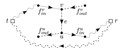
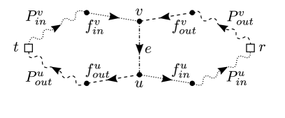
Figure 2: The case when $e=vu$ lies in both $A_{in}$ (dotted) and $A_{out}$ (dashed). Edges are straight lines, paths are wavy and may intersect. On the left: assuming that $A_{out}$ contains a path from the root $r$ to terminal $t$ that does not contain $e$ leads to a contradiction, since $f^{v}_{out}$ would then be redundant. On the right: otherwise, the paths connecting $r$ and $t$ with $v$ and $u$ imply the existence of a poly-cycle, which due to $e$ has a chord, again leading to a contradiction.

The in-arborescence $A_{in}$ contains a $t\to r$ path from some terminal $t\in R_{C}$ to the root $r$ passing through $e$. We claim that $A_{out}$ must contain an $r\to t$ path to the same terminal $t$ passing through $e$ as well. If this were not the case there would be some other $r\to t$ path of $A_{out}$ not containing $e$. Together with the $t\to v$ subpath of the $t\to r$ path in $A_{in}$, this implies an $r\to v$ path not containing $f^{v}_{out}$: the latter edge is not contained in $A_{in}$ and therefore cannot be part of the $t\to v$ subpath. However this means that every terminal reachable from $r$ via $v$ in $C^{\prime}$ is reachable by a path not containing $f^{v}_{out}$. As this edge is not contained in $A_{in}$, it could safely be removed from $C^{\prime}$ without disconnecting any terminal pair. This would contradict the minimality of $C^{\prime}$, which means there must be an $r\to t$ path in $A_{out}$ that passes through $v$.

For this terminal $t$, we can conclude that there is a $t\to v$ path $P^{v}_{in}\subseteq A_{in}$ ending in $f^{v}_{in}$, a $u\to r$ path $P^{u}_{in}\subseteq A_{in}$ starting in $f^{u}_{in}$, but also an $r\to v$ path $P^{v}_{out}\subseteq A_{out}$ ending in $f^{v}_{out}$, and a $u\to t$ path $P^{u}_{out}\subseteq A_{out}$ starting in $f^{u}_{out}$. Moreover, none of these four paths contains $e$. Note that the union $P^{v}_{in}\cup P^{u}_{in}\cup P^{v}_{out}\cup P^{u}_{out}$ of the four paths contains a poly-cycle $O$ for which $e$ is a chord, i.e., it connects two non-adjacent vertices of $O$.

The strongly connected component $C^{\prime}$ was constructed from the component $C$ of the optimum solution $N$ by adding the set $\widetilde{F}$ of reverse edges to some existing edge set $F$ of $C$. Hence, even if $O$ and/or $e$ do not exist in $N$, there still exists a poly-cycle $O^{\prime}$ in $N$ with the same vertex set and underlying undirected graph as $O$, and an edge $e^{\prime}$ that is a chord to $O^{\prime}$, which may be $e$ or its reverse edge. This contradicts the optimality of $N$ by Section 2.1, and thus $u\in N(v)$ is in $W$.

It remains to consider the case when $v$ has four incident edges. This means that for one neighbour $u$ of $v$ there are two edges $uv$ and $vu$ in $C^{\prime}$ of which one belongs to $A_{in}$ and the other to $A_{out}$. W.l.o.g., let $uv$ belong to $A_{out}$ (for the other case when $uv$ belongs to $A_{in}$, by symmetry an analogous argument to the following exists). Now let $w_{out}$ and $w_{in}$ be the other two neighbours of $v$, for which the edge $vw_{out}$ is in $A_{out}$, while the edge $w_{in}v$ is in $A_{in}$. If either $w_{in}$ or $w_{out}$ is in $W$, we are done. Hence assuming that $w_{in},w_{out}\notin W$, just as $v$, both $w_{in}$ and $w_{out}$ are Steiner vertices with three neighbours, each incident to two edges of $A_{in}$ and two edges of $A_{out}$. If either $w_{in}$ or $w_{out}$ has an incident edge that lies in the intersection of $A_{in}$ and $A_{out}$, by the same argument as for $v$ above, some vertex of $N(w_{in})\cup N(w_{out})$ must lie in $W$. As $N(w_{in})\cup N(w_{out})\subseteq N^{2}[v]$ this would conclude the proof.

Figure 3: The case when $vu$ lies in $A_{in}$ (dotted) and $uv$ lies in $A_{out}$ (dashed). Assuming that neither $w_{in}$ nor $w_{out}$ has an incident edge lying in both arborescences leads to a contradiction, since $vu$ being a bridge in $\overline{C^{\prime}}$ implies a path of $A_{in}$ (wavy) connecting $w_{out}$ with $x_{in}$, but $x_{in}w_{in}$ is also a bridge in $\overline{C^{\prime}}$.

Hence assume that neither $w_{in}$ nor $w_{out}$ has an incident edge lying in both arborescences. Thus $w_{out}$ has a neighbour $x_{out}\neq v$ such that $w_{out}x_{out}\in E(A_{out})$ and $x_{out}w_{out}\in E(A_{in})$, and $w_{in}$ has a neighbour $x_{in}\neq v$ such that $x_{in}w_{in}\in E(A_{in})$ and $w_{in}x_{in}\in E(A_{out})$. See Figure 3. Note that $x_{in}\neq x_{out}$ as otherwise $A_{in}$ would have a vertex of out-degree more than one. Moreover, by the following argument, we can conclude that in $\overline{C^{\prime}}$, all three undirected edges $vu$, $x_{out}w_{out}$, and $x_{in}w_{in}$ are bridges. Consider any edge $e$ in the component $C$ of the optimum solution $N$ from which $C^{\prime}$ was constructed. By Section 2.1, the reverse edge of $e$ can only exist in $C$ if $e$ does not lie on any poly-cycle. That is, if $e$ and its reverse edge exist in $C$ then the corresponding edge in $\overline{C}$ is a bridge. To obtain $C^{\prime}$ from $C$ we added $\widetilde{F}$, which contains all reverse edges of the condensation graph of $C$. From Section 4 we concluded that the condensation graph of $C$ is a poly-forest. Thus any edge of $C^{\prime}$ for which the reverse edge exists in $C^{\prime}$ as well, must correspond to a bridge in $\overline{C^{\prime}}$, including $vu$, $x_{out}w_{out}$, and $x_{in}w_{in}$, which all lie in $A_{in}$. Note also that by the same observations, $v$, $w_{out}$, and $w_{in}$ lie in the same $2$-connected component of $\overline{C^{\prime}}$, as the reverse edges of $vw_{out}$ and $w_{in}v$ do not exist in $C^{\prime}$.

This means that $A_{in}$ contains a path starting in $x_{out}w_{out}$, which reaches the root of $A_{in}$ by passing through $vu$, as the latter is a bridge of $\overline{C^{\prime}}$ while $v$ and $w_{out}$ lie in the same $2$-connected component of $\overline{C^{\prime}}$. Since neither $v$ nor $w_{in}$ is a branching point of $A_{in}$ while $x_{in}w_{in},w_{in}v,vu\in E(A_{in})$, this path of $A_{in}$ contains the subpath given by the sequence $x_{in}w_{in}vu$. But this means that there is a path from $x_{out}w_{out}$ to $x_{in}$ that does not pass through $w_{in}x_{in}\in A_{out}$. This contradicts the fact that $x_{in}w_{in}$ is a bridge of $\overline{C^{\prime}}$, and thus concludes the proof. $\lrcorner$

As the graph $G_{N}$ is bidirected, for any $v$-$u$ path $P$ in the underlying undirected graph $\overline{G}_{N}$ of $G_{N}$, there exists a corresponding directed $v\to u$ path in $G_{N}$ of the same cost. Therefore, we can ignore the directions of the edges in $C^{\prime}$ and the arborescences $A_{out}$ and $A_{in}$ to identify the paths $P_{v}$ for Steiner vertices $v$ of $N$. Thus we will only consider paths in the graphs $\overline{C^{\prime}}$, $\overline{A}_{out}$, and $\overline{A}_{in}$ from now on. In particular, we exploit the following observation found in [du1991better] (and also used by borchers-du) on undirected trees.

Claim ([du1991better, Lemma 3.2]).

For any undirected tree $T$ we can find a path $P_{v}\subseteq T$ for every branching point $v$, such that $P_{v}$ leads from $v$ to some leaf of $T$, and all these paths $P_{v}$ are pairwise edge-disjoint.

If a Steiner vertex $v$ of $C^{\prime}$ is a branching point of $A_{out}$ ($A_{in}$), we let $P_{v}$ be the corresponding path in $\overline{A}_{out}$ ($\overline{A}_{in}$) given by Section 4 from $v$ to some leaf of $A_{out}$ ($A_{in}$), which is a terminal. Note that paths in $\overline{A}_{in}$ may overlap with paths in $\overline{A}_{out}$. However any edge in the union of all the paths $P_{v}$ chosen so far is contained in at most two such paths, one for a branching point of $A_{out}$ and one for a branching point of $A_{in}$.

It remains to choose a path $P_{v}$ for every Steiner vertex $v$ that is neither a branching point of $A_{out}$ nor of $A_{in}$, i.e., for every vertex not in $W$. By Section 4 for any such vertex $v\notin W$ there is a vertex $u\in N^{2}[v]$ for which $u\in W$. If $u$ is a terminal, then the path $P_{v}$ is simply the edge $vu$ if $u\in N(v)$ or the corresponding path $vwu$ for some $w\in N(v)$ otherwise. If $u$ is not a terminal but a branching point of $A_{out}$ or $A_{in}$, then we chose a path $P_{u}$ for $u$ above. In this case, $P_{v}$ is the path contained in the walk given by extending the path $P_{u}$ by the edge $vu$ or the path $vwu$, respectively. Note that, as any vertex of $C^{\prime}$ has at most $3$ neighbours, any terminal or branching point $u\in W$ can be used in this way for some vertex $v\notin W$ at most nine times. Therefore any edge in the union of all chosen paths is contained in $O(1)$ paths. Consequently the total cost $\sum_{v\in V(N)\setminus R}\operatorname{cost}(P_{v})$ is $O(\operatorname{cost}(C^{\prime}))$, and as $\operatorname{cost}(C^{\prime})\leq 2\operatorname{cost}(C)$ we also get $\sum_{v\in V(N)\setminus R}\operatorname{cost}(P_{v})=O(\operatorname{cost}(C))$.

We may repeat these arguments for every weakly connected component of $N$ to obtain the lemma. ∎

Next we give the proof of Section 4, which shows that there are weighted weak $r$-divisions for planar graphs.

Proof of Section 4.

We will not be concerned with the edge weights of $N$ and accordingly define the distance function $d_{M}(u,v)$ for any subgraph $M$ of $N$ to be the hop-distance between $u$ and $v$ in $\overline{M}$, i.e., the minimum number of edges on any path from $u$ to $v$ in $\overline{M}$. The idea (as outlined in [KPR-Lee, fakcharoenphol2003improved]) is to iteratively “chop” the vertices of $N$ into disjoint sets that induce annuli of bounded thickness measured in the hop-distance, using the following random process. For a fixed value $\tau$, if we are given some connected graph $M$, then we first choose an offset $\tau_{0}\in\{1,\ldots,\tau\}$ uniformly at random and an arbitrary vertex $v_{0}$ of $M$. A so-called $\tau$-chop then is the partition of the vertices of $M$ defined by the sets A_0&={v∈V(M)∣d_M(v_0,v)¡τ_0} and
A_i={v∈V(M)∣τ_0+(i-1)τ≤d_M(v_0,v)¡τ_0+iτ} for i≥1.

We define a $\tau$-chop of a disconnected graph as the partition given by the union $\bigcup_{\ell}{\mathcal{P}}_{\ell}$ of $\tau$-chops ${\mathcal{P}}_{\ell}$, $\ell\geq 1$, of the connected components, where for each component we choose an offset $\tau_{0}$ uniformly at random and an arbitrary vertex $v_{0}$. Finally, a $\tau$-chop of a partition ${\mathcal{P}}$ is the refined partition given by the union of $\tau$-chops on each subgraph induced by a set in ${\mathcal{P}}$, again choosing a $v_{0}$ and a $\tau_{0}$ for every component of the subgraphs. Hence we may start with $N$ and iteratively perform $\tau$-chops to obtain smaller and smaller subsets of vertices.

KPR-Lee now proves the following claim, where the weak diameter of a subgraph $M\subseteq N$ is the maximum hop-distance of any two vertices of $M$ measured in the underlying graph $N$, i.e., $\max_{u,v\in V(M)}d_{N}(u,v)$. Note that this claim holds independent of the choices of the vertices $v_{0}$ and the offsets $\tau_{0}$.

Claim (Lemma 2 in [KPR-Lee]).

If $N$ excludes $K_{h}$ as a minor, then any sequence of $h-1$ iterated $\tau$-chops on $N$ results in a partition ${\mathcal{P}}$ of $V(N)$, such that each graph induced by a set $S\in{\mathcal{P}}$ has weak diameter $O(h\tau)$.

Let ${\mathcal{P}}$ be the partition of $V(N)$ from Section 4. Since $N$ is planar, it excludes $K_{5}$ as a minor, and so the weak diameter of each set $S\in{\mathcal{P}}$ is $O(\tau)$. We define a partition $\overline{{\mathcal{E}}}$ of the edges of $\overline{N}$, consisting of sets $E_{S}\subseteq E(\overline{N})$ for each $S\in{\mathcal{P}}$. In particular, if $S$ is the set containing the lexicographically smaller vertex incident to an edge $e$ of $\overline{N}$, then $e$ is contained in $E_{S}$. Note that the weak diameter of a region $M_{S}$ spanned by an edge set $E_{S}$ is at most the weak diameter of the graph induced by $S$ plus $2$, i.e., also the weak diameter of $M_{S}$ is $O(\tau)$. Since $\overline{N}$ has maximum degree $3$, the weak diameter bounds the number of vertices in each region by $|V(M_{S})|=2^{O(\tau)}$ for every $S\in{\mathcal{P}}$. As $\overline{{\mathcal{E}}}$ corresponds to a partition ${\mathcal{E}}$ of the edges of $N$, for some $\tau=\Theta(\log r)$ we obtain an $r$-division given by ${\mathcal{E}}$ with the required bound on the sizes of the regions.

It remains to bound the weight of the boundary vertices, for which we bound the expected weight among the random choices of offsets. More concretely, note that when performing a single $\tau$-chop on a connected graph $M$ from a fixed vertex $v_{0}$, two adjacent vertices $u,v$ end up in different sets $S$ with probability at most $1/\tau$ by the choice of the offset $\tau_{0}$ and the definition of the sets $A_{i}$, $i\geq 0$. We assign the edge $uv$ of $\overline{N}$ to the set $E_{S}$ containing the lexicographically smaller vertex among $u$ and $v$. Thus any vertex $w$, which has degree at most $3$ in $\overline{N}$, is a boundary vertex of a region spanned by some set $E_{S}$ with probability at most $3/\tau$ when performing a single $\tau$-chop from a fixed vertex $v_{0}$. As we perform $h-1=4$ iterative $\tau$-chops, the expected weight of the boundary vertices is at most $\frac{3\cdot 4}{\tau}\sum_{v\in V(N)}c(v)$. Hence, since $N$ is planar and by our choice of $\tau=\Theta(\log r)$, there exists an $r$-division with only a $O(1/\log r)$-fraction of the total vertex weight in the boundary vertices. ∎

Proving Section 4.

Finally, we can also prove that Theorem 4.1 implies a PSAKS for bi-DSN${}_{\textsc{Planar}}$, by utilizing some of the insights of the above proofs. The proof essentially follows the same lines as the one given for the ST problem by lokshtanov2017lossy based on the borchers-du Theorem.

Proof of Section 4.

To obtain a polynomial-sized $(1+{\varepsilon})$-approximate kernel we proceed similar to the algorithm described at the beginning of this section, by first computing an optimum solution for every possible pattern graph on at most $g({\varepsilon})=2^{1+1/{\varepsilon}}$ terminals from $R$. Using the XP algorithm of Theorem 1.4, this takes $n^{2^{O(1/{\varepsilon})}}$ time, as determined before. If ${\varepsilon}$ is a constant, this amounts to a polynomial runtime. Taking the union of all precomputed solutions gives a graph, which due to Theorem 4.1 contains a $(1+{\varepsilon})$-approximation to the optimum of the input graph $G$ (by the same arguments showing that the algorithm computes a $(1+{\varepsilon})$-approximation). However the union is not a kernel, since its size is not necessarily bounded as a function of the parameter $k$. In particular, it may contain many vertices and the edge weights might be large.

To reduce the number of vertices, we apply the vertex degree transformations from Section 2.2 to each computed optimum solution $N_{H^{\prime}}$ to patterns $H^{\prime}$ on at most $g({\varepsilon})$ terminals. In particular, every Steiner vertex of $N_{H^{\prime}}$ now has exactly three neighbours. We use the insights from the proof of Section 4 to argue that $N_{H^{\prime}}$ has a bounded number of vertices. By Section 4 we may assume that $N_{H^{\prime}}$ is an optimum solution to $H^{\prime}$ for which the condensation graph is a poly-forest. Now consider a weakly connected component $C$ of $N_{H^{\prime}}$. As argued in the proof of Section 4, if we add to $C$ the edge set $\widetilde{F}$, which contains the reverse edges to those of the condensation graph of $C$, then we obtain a minimal SCSS solution $C^{\prime}$ for the terminal set $R_{C}\subseteq R$ contained in $C$. This means that $C^{\prime}$ is the union of an in-arborescence $A_{in}$ and an out-arborescence $A_{out}$, both rooted at some terminal $r\in R_{C}$ and with leaves from $R_{C}$. The number of branching points of each of these arborescences is at most $|R_{C}|$. Hence the set $W$ (as defined earlier) of branching points and terminals $R_{C}$ contains at most $3|R_{C}|$ vertices. Due to Section 4 we can map any vertex not contained in $W$ to a vertex in $W$ at hop-distance at most $2$. Since every vertex not in $W$ is a Steiner vertex and has three neighbours, at most $9$ vertices map to any particular vertex of $W$. Thus the number of vertices of $C$ not in $W$ is at most $27|R_{C}|$, which brings the total to at most $30|R_{C}|$ after adding $W$. This means that the number of vertices of $N_{H^{\prime}}$ is at most $30g({\varepsilon})=2^{O(1/{\varepsilon})}$. As calculated earlier, the total number of pattern graphs $H^{\prime}$ on at most $g({\varepsilon})$ terminals is $k^{2^{O(1/{\varepsilon})}}$. Hence taking the union of all computed solutions $N_{H^{\prime}}$ after applying the vertex degree transformations of Section 2.2 gives a graph $G^{\prime}$ with $2^{O(1/{\varepsilon})}\cdot k^{2^{O(1/{\varepsilon})}}=k^{2^{O(1/{\varepsilon})}}$ vertices, which is polynomial in the parameter $k$ if ${\varepsilon}$ is constant.

For the edge weights, lokshtanov2017lossy show how to round them in such a way that each edge weight can be stored using $O(\log(k/{\varepsilon}))$ bits for the ST problem. Here we will need slightly more bits. As an ingredient we use that a polynomial time constant approximation algorithm exists, which is provided by Theorem 1.6. In particular, let $M\subseteq G$ be a $4$-approximate solution computed by this algorithm for the input graph $G$. If the weight of an edge $e$ of the union graph $G^{\prime}$ currently is $w(e)$, then we define a rounded integer weight ^w(e)=⌊—E(G’)—w(e)εcost(M) ⌋, and set the edge weights of the union graph $G^{\prime}$ to $\widehat{w}(e)$ instead. By Section 3 we have $\operatorname{cost}(N)\leq 2\operatorname{cost}(M)$ for the optimum planar solution $N$ to the input instance, and so we may remove any edge of cost more than $2\operatorname{cost}(M)$. This implies that $\widehat{w}(e)\leq 2|E(G^{\prime})|/{\varepsilon}$, which asymptotically is $k^{2^{O(1/{\varepsilon})}}$, as the graph $G^{\prime}$ has $k^{2^{O(1/{\varepsilon})}}$ vertices. Hence each edge weight can be encoded using $2^{O(1/{\varepsilon})}\log(k)$ bits, and the size of the kernel including the edge weights is $k^{2^{O(1/{\varepsilon})}}$.

It remains to show that rounding the edge weights does not distort the solution costs by too much. Let $N^{\prime}\subseteq G^{\prime}$ be a $\beta$-approximation of the optimum planar solution in the kernel, i.e., using weights $\widehat{w}(e)$. Let also $N^{\star}$ be the optimum planar solution in $G^{\prime}$ when using the original weights $w(e)$. In particular, we get $\sum_{e\in E(N^{\prime})}\widehat{w}(e)\leq\beta\sum_{e\in E(N^{\star})}\widehat{w}(e)$, since the optimum planar solution in the kernel has cost at most that of $N^{\star}$ according to weights $\widehat{w}(e)$. Since $N^{\prime}$ has at most as many edges as $G^{\prime}$, the cost of $N^{\prime}$ measured by the original edge weights $w(e)$ compared to $N^{\star}$ and $M$ is ∑_e∈E(N’) w(e) &≤∑_e∈E(N’)