Dispersive readout of adiabatic phases

Abstract

We propose a protocol for the measurement of adiabatic phases of periodically driven quantum systems coupled to an open cavity that enables dispersive readout. It turns out that the cavity transmission exhibits peaks at frequencies determined by a resonance condition that involves the dynamical and the geometric phase. Since these phases scale differently with the driving frequency, one can determine them by fitting the peak positions to the theoretically expected behavior. For the derivation of the resonance condition and for a numerical study, we develop a Floquet theory for the dispersive readout of ac-driven quantum systems. The feasibility is demonstrated for two test cases that generalize Landau-Zener-Stückelberg-Majorana interference to two-parameter driving.

A state vector that undergoes a cyclic evolution in Hilbert space acquires a phase factor that can be divided into a dynamical and a geometric part Aharonov and Anandan (1987). The latter is gauge invariant and in the adiabatic limit agrees with the phase discovered earlier by Berry for cyclic adiabatic following Berry (1984). Ever since these phases have attracted much attention owing to their fundamental significance as well as for the their usefulness for, e.g., computing electronic properties of solids Xiao et al. (2010). The Floquet states of an ac driven system are periodic in time and describe a cyclic solution of the time-dependent Schrödinger equation Shirley (1965); Sambe (1973). Moreover, they can be characterized by a mean energy which is essentially the dynamical phase, while the geometric phase corresponds to the difference between the quasienergy and the mean energy Moore (1990); Grifoni and Hänggi (1998).

The direct observation of geometric phases is hindered by two obstacles. First, phases are commonly visible in interference effects that depend on the relative phase of a superposition. Second, interference is sensitive to the total phase without distinguishing between a dynamical and a geometric contribution. Therefore, measuring geometric phases requires the construction of a Hamiltonian for which the dynamical phase vanishes Unanyan and Fleischhauer (2004). This can be accomplished also dynamically by spin-echo ideas by which a $\pi$-pulse inverts the Bloch vector after half a driving period Falci et al. (2000); Peng et al. (2006); Leek et al. (2007). The present work proposes a measurement scheme for geometric phases which differs from previous ones in the way the dynamical and the geometric phase are disentangled.

Landau-Zener-Stückelberg-Majorana (LZSM) interference in solid-state qubits Shevchenko et al. (2010) is achieved by driving a qubit such that its excitation probability as a function of the detuning and the driving amplitude exhibits a characteristic pattern. The common one-parameter driving, however, restricts the adiabatic phases to multiples of $2\pi$, despite that beyond the adiabatic limit non-trivial geometric phases may emerge. Since LZSM interferometry became an established experimental technique, it is natural to use it as starting point and to extend it by a second driving that enables non-trivial adiabatic phases.

To gain information about a qubit, one frequently employs dispersive readout based on the coupling to a cavity. Then the cavity experiences a frequency shift which depends on the qubit state and can be probed via the transmission Blais et al. (2004). Theoretically this can be seen in the qubit-cavity Hamiltonian after a transformation to the dispersive frame Blais et al. (2004); Zueco et al. (2009). In a more systematic and generalizable treatment, one relates the cavity transmission to the susceptibility of the qubit coupled to it Petersson et al. (2012); Burkard and Petta (2016).

Here we generalize the theory of dispersive readout to ac driven quantum systems. We will find that the cavity transmission as a function of the driving frequency exhibits regularly spaced peaks. Their distances relate to the Berry phases of the adiabatic eigenstates.

Dispersive readout of a driven system.—We consider a driven quantum system, henceforth “qubit”, with the $T$-periodic Hamiltonian $H_{\text{qb}}(t)$ and the driving frequency $\Omega=2\pi/T$. Decoherence is taken into account by employing a quantum master equation that starts from the qubit-bath Hamiltonian $H_{\text{qb-bath}}=X\sum_{\nu}\lambda_{\nu}(b_{\nu}^{\dagger}+b_{\nu})$, with $b_{\nu}$ describing the modes of a bosonic environment Leggett et al. (1987); Hänggi et al. (1990), for details see Appendix B. Dispersive readout Blais et al. (2004) is enabled by coupling the qubit to an open cavity such that the central Hamiltonian reads (in units with $\hbar=1$)

$$H=H_{\text{qb}}(t)+gZ(a^{\dagger}+a)+\omega_{0}a^{\dagger}a$$ (1)

with a qubit operator $Z$ and $a$ the usual bosonic annihilation operator of the cavity mode. The cavity couples at both ends $\nu=1,2$ to incoming and outgoing modes. Starting again from a system-bath model, one can employ input-output theory Collett and Gardiner (1984); Gardiner and Zoller (2004); Clerk et al. (2010) to obtain the quantum Langevin equation

$$\dot{a}_{t}=-i\omega_{0}a_{t}-\frac{\kappa}{2}a_{t}-\sum_{\nu=1,2}\sqrt{\kappa_{\nu}}a_{\text{in},\nu}-igZ_{t}$$ (2)

with the input fields $a_{\text{in},\nu}$ and the cavity loss rate $\kappa=\kappa_{1}+\kappa_{2}$. The corresponding time-reversed equation provides the input-output relation $a_{\text{in},\nu}+a_{\text{out},\nu}=\sqrt{\kappa_{\nu}}a$ and the cavity transmission which contains information about the qubit.

In turn, the qubit experiences a force from the cavity which can be derived (see Appendix A) from linear response theory to read

$$\langle Z_{t}\rangle=g\int dt^{\prime}\,\chi(t,t^{\prime})\langle a^{\dagger}_{t^{\prime}}+a_{t^{\prime}}\rangle\,.$$ (3)

The susceptibility $\chi(t,t^{\prime})=-i\langle[Z(t),Z(t^{\prime})]\rangle^{(0)}\theta(t-t^{\prime})$ has to be evaluated at time $t^{\prime}$ in the absence of the cavity. Generally for time-dependent systems, such expressions depend explicitly on both times, while for periodic driving, $\chi(t,t^{\prime})=\chi(t+T,t^{\prime}+T)$. Consequently, upon introducing the time difference $\tau=t-t^{\prime}$ we find that $\chi(t,t-\tau)$ is $T$-periodic in $t$ Kohler et al. (2005) and, thus, can be written as

$$\chi(t,t-\tau)=\sum_{k}\int\frac{d\omega}{2\pi}\,e^{-ik\Omega t-i\omega\tau}\chi^{(k)}(\omega)\,.$$ (4)

This implies for Eq. (3) the Fourier representation $Z_{\omega}=g\sum_{k}\chi^{(k)}(\omega-k\Omega)(a_{\omega-k\Omega}+a^{\dagger}_{\omega-k\Omega})$ which reflects the frequency mixing inherent in the linear response of the driven quantum system.

Since $a_{\omega}$ has its dominating contribution at the bare cavity frequency $\omega_{0}$, the qubit response $Z_{\omega}$ mainly contains the frequencies $\pm\omega_{0}+k\Omega$, where contributions with $-\omega_{0}$ stem from the creation operator $a^{\dagger}_{\omega}$. For the backaction of the qubit to the oscillator, the component with frequency $\omega_{0}$ represents the only resonant excitation. In the good cavity limit $\kappa\ll\omega_{0},\Omega$, we can neglect within a rotating-wave approximation all non-resonant components, which means that the relevant qubit response is given by $Z_{\omega}=g\chi^{(0)}(\omega)a_{\omega}$. Inserting this result into Eq. (2), we obtain via Fourier transformation an expression for $a_{\omega}$. Together with the input-output relation follows the cavity transmission amplitude

$$t_{c}=\frac{\langle a_{\text{out},2}\rangle}{\langle a_{\text{in},1}\rangle}=\frac{i\sqrt{\kappa_{1}\kappa_{2}}}{\omega_{0}-\omega+g^{2}\chi^{(0)}(\omega)-i\kappa/2}.$$ (5)

Its dependence on $\chi$ allows one to acquire information about the qubit by probing the transmission $|t_{c}|^{2}$ Blais et al. (2004) (for graphical reasons, the reflection $R=1-|t_{c}|^{2}$ will be plotted).

Floquet theory.—The remaining task is the computation of $\chi^{(0)}(\omega)$. To this end, we employ the Floquet-Markov formalism developed in Ref. Kohler et al. (1997). It starts by diagonalizing $H_{\text{qb}}(t)-i\partial_{t}$ in the Hilbert space extended by the space of $T$-periodic functions Shirley (1965); Sambe (1973) to obtain the Floquet states $|\phi_{\alpha}(t)\rangle=|\phi_{\alpha}(t+T)\rangle$, the quasienergies $\epsilon_{\alpha}$, the mean energies $\bar{E}_{\alpha}$, and the stationary solutions of the Schrödinger equation, $|\psi_{\alpha}(t)\rangle=e^{-i\epsilon_{\alpha}t}|\phi_{\alpha}(t)\rangle$. The corresponding expression for the propagator, $U(t,t^{\prime})=\sum_{\alpha}e^{-i\epsilon_{\alpha}(t-t^{\prime})}|\phi_{\alpha}(t)\rangle\langle\phi_{\alpha}(t^{\prime})|$, allows us to deal with the interaction picture operators in $\chi(t,t^{\prime})$. Moreover, the Floquet states provide a convenient basis for the Bloch-Redfield master equation Redfield (1957); Blum (1996) for the qubit density operator which in this representation eventually becomes diagonal Kohler et al. (1997), $\rho_{\text{qb}}=\sum p_{\alpha}|\phi_{\alpha}(t)\rangle\langle\phi_{\alpha}(t)|$. In contrast to a static system, the probabilities $p_{\alpha}$ at long times are not simple Boltzmann factors.

With these ingredients, we find from Eq. (4) the susceptibility,

$$\chi^{(0)}(\omega)=\sum_{\beta,\alpha,k}\frac{(p_{\alpha}-p_{\beta})|Z_{\beta\alpha,k}|^{2}}{\omega+\epsilon_{\alpha}-\epsilon_{\beta}+k\Omega+i\gamma/2},$$ (6)

where $Z_{\beta\alpha,k}$ denotes the $k$th Fourier component of the $T$-periodic transition matrix element $Z_{\beta\alpha}(t)=\langle\phi_{\beta}(t)|Z|\phi_{\alpha}(t)\rangle$. To regularize the Fourier integrals, we have introduced the phenomenological level broadening $\gamma$ of the Floquet states.

Equation (5) together with Eq. (6) represents a generalization of dispersive readout to quantum systems under strong ac driving (in addition to the weak driving entailed by $a_{\text{in},1}$ via the cavity). For details of the derivation, see Appendix B.

Resonance condition, geometric phase, and adiabatic limit.—Upon resonant driving of the cavity with frequency $\omega=\omega_{0}$, the reflection $R$ assumes its maximum when the real part of the susceptibility (6) vanishes. This is the case when the quasienergies and the driving frequency obey the condition

$$\epsilon_{\beta}-\epsilon_{\alpha}=\omega_{0}+k\Omega_{k},$$ (7)

where $\Omega_{k}$ is the $k$th resonance (notice that smaller $\Omega_{k}$ have larger index).

The second cornerstone of our protocol stems from the relation between Floquet states and geometric phases. The former are time-periodic and during each cycle they acquire the phase $\epsilon_{\alpha}T=\bar{E}_{\alpha}T-\gamma_{\alpha}$, where $\gamma_{\alpha}=\int_{0}^{T}dt\langle\phi_{\alpha}(t)|i\partial_{t}|\phi_{\alpha}(t)\rangle$ is the (non-adiabatic) geometric phase of the Floquet state $|\phi_{\alpha}(t)\rangle$ Aharonov and Anandan (1987); Moore (1990); Grifoni and Hänggi (1998). To avoid difficulties with the quasienergies for small frequencies Hone et al. (1997), we substitute the $\epsilon_{\alpha}$ by $\bar{E}_{\alpha}-\gamma_{\alpha}/T$, where both $\bar{E}_{\alpha}$ and $\gamma_{\alpha}$ have a well-defined adiabatic limit in which $\gamma_{\alpha}$ becomes the Berry phase Aharonov and Anandan (1987); Moore (1990). Then the resonance condition (7) becomes

$$\frac{1}{\Omega_{k}}=C_{\beta\alpha}\Big{(}k+\frac{\gamma_{\beta\alpha}}{2\pi}\Big{)}$$ (8)

with $C_{\beta\alpha}=(\bar{E}_{\beta}-\bar{E}_{\alpha}-\omega_{0})^{-1}$ and the geometric phase $\gamma_{\beta\alpha}\equiv\gamma_{\beta}-\gamma_{\alpha}$.

This result suggests for the dispersive readout of adiabatic phases the following strategy. One considers low frequencies, such that the terms on the right-hand side of Eq. (8) assume their adiabatic limit (possible corrections are of the order $\Omega$). Then the cavity reflection $R(\Omega)$ exhibits peaks whose positions as a function of their index $k$ can be fitted to the expected linear behavior. This provides the adiabatic phase $\gamma_{\beta\alpha}$, the coefficient $C_{\beta\alpha}$ and, thus, the dynamical phase $-(\bar{E}_{\beta}-\bar{E}_{\alpha})T$. The index $k$ of the probed resonances may contain an offset $k_{0}$ which is irrelevant, because it changes $\gamma_{\beta\alpha}$ merely by an irrelevant multiple of $2\pi$.

In the low-frequency limit, the system will eventually reside in the Floquet state with the smallest mean energy, labelled with $\alpha=0$. Then dispersive readout probes the geometric phases $\gamma_{\beta 0}=\gamma_{\beta}-\gamma_{0}$.

Two-level system as test case.—The paradigmatic example for a Berry phase is the one of a two-level system with the pseudo-spin Hamiltonian $H_{\text{qb}}=\frac{1}{2}\mathbf{B}(t)\cdot\bm{\sigma}$ and the periodically time-dependent “magnetic field” $\mathbf{B}(t+T)=\mathbf{B}(t)$. As is well known Sakurai (1995), the adiabatic ground state of $H_{\text{qb}}$ acquires a geometric phase that equals the solid angle of the curve $\mathbf{B}(t)$ with respect to the origin. This implies that for a smooth behavior of the adiabatic phase as a function of a control parameter, $H_{\text{qb}}(t)$ must contain all three Pauli matrices. Let us therefore consider the qubit Hamiltonian

$$H_{\text{qb}}(t)=\frac{\Delta}{2}\sigma_{x}+\frac{\epsilon}{2}\sigma_{z}+A\sigma_{z}\cos(\Omega t)+B\sigma_{y}\sin(\Omega t)$$ (9)

with tunnel matrix element $\Delta$, detuning $\epsilon$, and driving amplitudes $A$ and $B$. For $B=0$ this model has been widely studied in the context of LZSM interference Shevchenko et al. (2010). To complete the model, we choose for the qubit-cavity coupling the operator $Z=\sigma_{z}$, while the qubit-bath interaction is specified by $X=\sigma_{x}$.

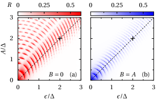
Figure 1: Reflection of the resonantly excited cavity as a function of the detuning and the amplitude for one-parameter driving (a) and two-parameter driving (b) of the qubit with frequency $\Omega=0.1\Delta$. Cavity frequency and line width are $\omega_{0}=0.95\Delta$ and $\kappa=\omega_{0}/1000$, while the coupling constants to the qubit and the bath read $g=0.005\Delta$ and $\alpha=0.01$. Crosses and dashed lines mark the values used in Figs. 2 and 3(a), respectively.

For later comparison, we start with one-parameter driving ($B=0$) for which $\gamma_{10}$ vanishes. Figure 1(a) shows the resulting cavity reflection as a function of the detuning and the driving amplitude. It has the typical shape of a low-frequency LZSM interference pattern Shevchenko et al. (2010). For two-parameter driving with equal amplitudes, $B=A$, [Fig. 1(b)], only the resonances close to $A\approx|\epsilon|$ are well visible. Henceforth we concentrate on this region.

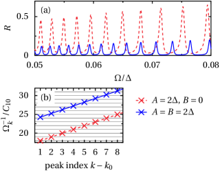
Figure 2: (a) Cavity reflection as a function of the driving frequency for one-parameter (dashed) and two-parameter driving (solid) with $A=\epsilon=2\Delta$. All other parameters are as in Fig. 1. (b) Corresponding reciprocal peak positions as a function of their index with an unknown offset $k_{0}$. The scaling factor $C_{10}$ stems from fitting the data to Eq. (8) with $\gamma_{10}$ as a second fit parameter. The vanishing Berry phases for one-parameter driving correspond to integer values marked by horizontal lines. Lines connecting the crosses are a guide to the eye.

According to our readout protocol, we consider fixed parameters and amplitudes and vary the driving frequency. The resulting cavity reflection [Fig. 2(a)] exhibits non-equidistant peaks. We fit their positions to the behavior predicted by Eq. (8) and, in doing so, determine from the spectrum both $C_{10}$ and the adiabatic phase $\gamma_{10}$. The accordingly scaled inverse peak positions are analyzed in Fig. 2(b). For one-parameter driving, they assume integer values in agreement with the fact that the adiabatic phases are multiples of $2\pi$. For two-parameter driving, according to Eq. (8), the values are shifted to non-integer values.

To verify that adiabatic phases can be obtained in a broad parameter range by the measurement of spectra such as the one in Fig. 2(a), we repeat this procedure for the amplitudes and detunings marked in Fig. 1 by dashed lines. The symbols in Fig. 3(a) depict the phases reconstructed in this way. The lines, by contrast, are obtained by diagonalizing $H_{\text{qb}}(t)$ and numerically evaluating $\gamma_{\alpha}^{\text{ad}}=\int_{0}^{T}dt\langle u_{\alpha}(t)|i\partial_{t}|u_{\alpha}(t)\rangle$ for each adiabatic eigenstate $|u_{\alpha}(t)\rangle$ on_ ; Simon and Mukunda (1993).

Typically the “measurement” deviates from the theoretically expected values by up to $0.03\pi$. This difference diminishes with smaller driving frequency [see inset of Fig. 3(a)] and therefore can be attributed mainly to non-adiabatic corrections. Moreover, for tiny driving amplitudes, the resonance peaks may not be very pronounced such that their positions cannot be determined well. Nevertheless, the numerical simulation of the experiment confirms the main message of this work, namely that the smooth growth of $\gamma_{10}$ with the amplitudes $A$ and $B$ can be determined from the resonance peaks in the dispersive readout, even when the system is not operated in the very deep adiabatic regime.

It is worthwhile to estimate the precision required in a possible experiment. In the fitting procedure, one determines $k+\gamma_{10}/2\pi=(\Omega_{k}C_{10})^{-1}$ for $k\sim 20$ and $0\leq|\gamma_{10}|<2\pi$. Hence, to identify $\gamma_{10}$ with a deviation clearly below $2\pi$, the relative error of the peak positions $\Omega_{k}$ should not exceed 1%. Then the accurracy is roughly as in the experiment of Ref. Leek et al. (2007).

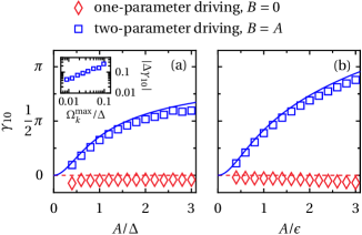
Figure 3: (a) Adiabatic phases as a function of the driving amplitude $A$ for the detuning $\epsilon=A$ marked in Fig. 1 by dashed lines. The symbols depict the values reconstructed from the positions of the first 10 resonance peaks with $\Omega<0.05\Delta$. The lines correspond to $\gamma_{10}^{\text{ad}}$ computed with the adiabatic eigenstates of $H_{\text{qb}}(t)$. Inset: Deviation $|\gamma_{10}-\gamma_{10}^{\text{ad}}|$ as a function of the largest $\Omega_{k}$ used for the fitting at $A=B=\epsilon=2\Delta$. (b) Corresponding plot for the alternative Hamiltonian (10) for constant detuning $\epsilon$ as a function of the driving amplitude $A$ with the tunneling $\Delta=A/1.2$.

Qubit with time-dependent tunnel phase.—As an alternative setup, we consider the Hamiltonian

$$H_{\text{qb}}^{\prime}(t)=\frac{\Delta}{2}\sigma_{x}+\frac{\epsilon}{2}\sigma_{z}+A\sigma_{x}\cos(\Omega t)-B\sigma_{y}\sin(\Omega t)\,,$$ (10)

where $\sigma_{z}$ refers to the charge degree of freedom, while $\sigma_{x}$ and $\sigma_{y}$ describe tunneling. Thus for $A=B$, the driving in Eq. (10) corresponds to a tunnel matrix element $\propto\exp(i\Omega t)$. This can be achieved with two quantum dots that are connected by two independent paths Gustavsson et al. (2007). Then a time-dependent flux between paths yields the driving in $H_{\text{qb}}^{\prime}(t)$. A further implementation has been proposed Falci et al. (2000); Peng et al. (2006) and realized Leek et al. (2007) by driving a qubit resonantly with a signal that possesses a linearly growing phase.

Since the driving couples to $\sigma_{x}$, we now keep the detuning $\epsilon$ fixed and vary the static tunneling $\Delta$. The resulting LZSM patterns are similar to those in Fig. 1, but with the main resonance lines for slightly larger amplitudes (see Appendix C). The directly computed adiabatic phase and the one extracted from the peak positions are compared in Fig. 3(b). Their agreement is similar to the one found for $H_{\text{qb}}(t)$.

Conclusions.—We have proposed a protocol for the dispersive readout of adiabatic phases of time-dependent quantum systems. Its main difference to previous proposals Unanyan and Fleischhauer (2004); Falci et al. (2000); Peng et al. (2006) and experiments Leek et al. (2007) lies in the treatment of the dynamical phase. While former works employed spin echo ideas or sophisticated Hamiltonians to physically eliminate the dynamical phase from the quantum dynamics, the present scheme provides the values of both phases from an analysis of the resonance spectrum. Therefore the protocol is applicable even when a dynamical phase cannot be avoided or reversed. The essential ingredients are, first, that the dynamical and the adiabatic phase as a function of the driving frequency scale differently and, second, that the resonance condition for dispersive readout of a driven quantum system can be expressed in terms of these phases. The importance of the scaling behavior relates the scheme to a proposal for measuring Chern numbers by considering the response of a quantum system to a quench as a function of the velocity at which the parameters are changed Gritsev and Polkovnikov (2012); Schroer et al. (2014). There, however, the measurement relies on a more involved quantum state tomography. Here, by contrast, the conceptually simpler dispersive readout signal is sufficient.

We have demonstrated the feasibility of the protocol by its numerical simulation for realistic solid-state qubits. The results indicate that even though the system is not operated in the deep adiabatic regime, present technology allows recovering the phases with a precision of roughly $\pi/30$ as follows from a rather conservative estimate. This may be improved by employing future qubits with less decoherence which enables smaller driving frequencies and yields sharper peaks.

For the theoretical description, we have developed a Floquet approach for the dispersive readout of periodically driven quantum systems. Its cornerstone is the identification of the relevant Fourier component of the qubit susceptibility. This theory was essential in two respects. First, it allowed the computation of the cavity reflection. Second, it provided insight to the measurement of driven quantum system as well as the resonance condition for the peaks in the transmission spectrum.

The recent experimental success with the dispersive readout of qubits in the context of LZSM interference indicates the feasibility of similar measurements with a second driving parameter. In turn, the prospects of observing in this way not only novel interference patterns, but also a quantity of fundamental interest such as the Berry phase may motivate researchers to attempt such experiments.

Appendix A Response of a strongly driven qubit to an additional weak driving

We consider a strongly driven quantum system with the time-dependent Hamiltonian $H_{0}(t)$ and a coupling to a heat bath. Then generally the reduced density operator $\rho_{0}(t)$ is time-dependent as well and may describe a situation far from equilibrium. In addition, the system is weakly driven by a force $f(t)$ entering via an operator $Y$, such that the Hamiltonian becomes $H(t)=H_{0}(t)+Yf(t)$. In an interaction picture that captures all influences but the weak additional driving, the Liouville-von Neumann equation reads $\dot{\rho}=-i[Y(t),\rho]f(t)$. Its integrated form provides the first-order solution

$$\rho(t)=\rho_{0}(t)-i\int_{-\infty}^{t}dt^{\prime}\,[Y(t^{\prime}),\rho_{0}(t^{\prime})]f(t^{\prime})\,,$$ (11)

such that the expectation value of an operator $Z$ reads

$$\langle Z_{t}\rangle=\langle Z_{t}\rangle^{(0)}+\int dt^{\prime}\,\chi(t,t^{\prime})f(t^{\prime})$$ (12)

with the susceptibility

$$\chi(t,t^{\prime})=-i\langle[Z(t),Y(t^{\prime})]\rangle_{t^{\prime}}^{(0)}\theta(t-t^{\prime})\,.$$ (13)

Formally, this is the usual Kubo formula, but with the equilibrium density operator replaced by the non-equilibrium $\rho_{0}(t^{\prime})$ which may depend on the dynamics of the strongly driven qubit as well as on its initial state. The latter is already the case for the usual dispersive readout Blais et al. (2004) by which one determines whether the qubit is initially in the ground state or in the excited state. Notice that the susceptibility $\chi(t,t^{\prime})$ depends explicitly on both times such that the integral in Eq. (12) generally is not a mere convolution.

Appendix B Susceptibility of a periodically driven system

If the Hamiltonian $H_{0}(t)$ is $T$-periodic, two-time expectation values such as the susceptibility in the long-time limit are invariant under a shift of both times, $\chi(t,t^{\prime})=\chi(t+T,t^{\prime}+T)$. Then introducing the time difference $\tau=t-t^{\prime}$ yields $\chi(t,t-\tau)=\chi(t+T,t+T-\tau)$. Consequently, the frequency representation of $\chi(t,t-\tau)$ can be written as a Fourier series in $t$, while the $\tau$-dependence still requires a Fourier integral Kohler et al. (2005). Therefore,

$$\chi(t,t-\tau)=\sum_{k}\int\frac{d\omega}{2\pi}e^{-ik\Omega t}e^{-i\omega\tau}\chi^{(k)}(\omega)$$ (14)

with $\Omega=2\pi/T$. Inserting this expression into Eq. (12) results in the linear response formula in Fourier space,

$$Z_{\omega}=Z_{\omega}^{(0)}+\sum_{k}\chi^{(k)}(\omega-k\Omega)f_{\omega-k\Omega}\,.$$ (15)

It reveals that the reaction of a periodically driven quantum system to a weak probe $f(t)$ is characterized by frequency mixing with sidebands separated by the frequency $\Omega$ of the strong driving.

B.1 Floquet theory

The explicit computation of the susceptibility may still be a formidable task. Here, we perform it within the Floquet-Markov approach of Refs. Kohler et al. (1997); Blattmann et al. (2015). It starts from a system-bath model Leggett et al. (1987); Hänggi et al. (1990) in which the qubit couples to an ensemble of harmonic oscillators described by the Hamiltonian $H_{\text{bath}}=\sum_{\nu}\hbar\omega_{\nu}b_{\nu}^{\dagger}b_{\nu}$, where $b_{\nu}$ is the usual bosonic annihilation operator of an oscillator with frequency $\omega_{\nu}$. The bath oscillators couple to a qubit operator $X$ according to the Hamiltonian

$$H_{\text{qb-bath}}=X\sum_{\nu}\lambda_{\nu}(b_{\nu}^{\dagger}+b_{\nu})\,.$$ (16)

The influence of the bath can be captured by its spectral density $J(\omega)=\pi\sum_{\nu}|\lambda_{\nu}|^{2}\delta(\omega-\omega_{\nu})\equiv J(\omega)=\pi\alpha\omega/2$ with the dimensionless coupling strength $\alpha$ Leggett et al. (1987); Hänggi et al. (1990). Within second-order perturbation theory one finds for the reduced qubit density operator the Bloch-Redfield master equation Redfield (1957); Blum (1996)

$$\begin{split}\dot{\rho}={}&-i[H_{\text{qb}}(t),\rho]\\ &-\int_{0}^{\infty}d\tau\big{\langle}[H_{\text{qb-bath}},[\tilde{H}_{\text{qb-bath}}(t,t-\tau),\rho]\big{\rangle}_{\text{bath,eq}}.\end{split}$$ (17)

For rather weak dissipation, $\rho(t)$ eventually becomes diagonal in the (time-dependent) basis of the Floquet states,

$$\rho_{0}(t)=\sum_{\alpha}p_{\alpha}|\phi_{\alpha}(t)\rangle\langle\phi_{\alpha}(t)|\,,$$ (18)

with the occupation probabilities $p_{\alpha}$. For this diagonal ansatz, the first term in Eq. (17) vanishes such that one obtains the Pauli-type master equation

$$\dot{p}_{\alpha}=\sum_{\beta}\big{(}W_{\alpha\leftarrow\beta}p_{\beta}-W_{\beta\leftarrow\alpha}p_{\alpha}\big{)}$$ (19)

with the generalized golden-rule rates

$$W_{\beta\leftarrow\alpha}=2\sum_{k}\big{|}X_{\beta\alpha,k}\big{|}^{2}N(\epsilon_{\beta}-\epsilon_{\alpha}-k\Omega),$$ (20)

and the Fourier components of the transitions matrix elements,

$$X_{\beta\alpha,k}=\int_{0}^{T}\frac{dt}{T}\,e^{ik\Omega t}\langle\phi_{\beta}(t)|X|\phi_{\alpha}(t)\rangle\,.$$ (21)

The function $N(\omega)=J(\omega)n_{\text{th}}(\omega)$ contains the bosonic thermal occupation number $n_{\text{th}}(\omega)=[e^{\hbar\omega/k_{B}T}-1]^{-1}$. In order to arrive at this concise form, we have defined the spectral density for negative $\omega$ as $J(\omega)=-J(-\omega)$, while the Bose function has been extended by analytic continuation.

Having obtained the time-independent long-time solutions for the probabilities $p_{\alpha}$, we can straightforwardly evaluate the susceptibility (14) which for $Y=Z$ results in the Fourier components

$$\chi^{(k)}(\omega)=\sum_{\alpha,\beta,k^{\prime}}\frac{(p_{\alpha}-p_{\beta})Z^{*}_{\beta\alpha,k^{\prime}-k}Z_{\beta\alpha,k^{\prime}}}{\omega+\epsilon_{\alpha}-\epsilon_{\beta}+k^{\prime}\Omega+i\gamma/2}\,,$$ (22)

where the matrix elements $Z_{\beta\alpha,k}$ are defined according to the $X_{\beta\alpha,k}$ in Eq. (21).

B.2 Limit of adiabatic following

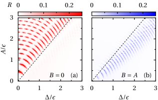
Figure 4: Cavity reflection for the alternative Hamiltonian $H_{\text{qb}}^{\prime}(t)$ for one-parameter driving with $B=0$ (a) and two-parameter driving with $B=A$ (b). Here the detuning $\epsilon$ is kept constant, while the tunneling $\Delta$ is varied. All other parameters are as in Fig. 1. The dashed lines mark the values used in Fig. 3(b).

It is instructive to relate the susceptibility (22) to the corresponding expression in the adiabatic limit based on the adiabatic solutions of the Schrödinger equation,

$$|\psi_{\alpha}(t)\rangle=e^{i\varphi_{\alpha}(t)}|u_{\alpha}(t)\rangle\,,$$ (23)

where the phase of each adiabatic eigenstate $|u_{\alpha}(t)\rangle$ is determined by $\dot{\varphi}_{\alpha}=\langle u_{\alpha}(t)|i\partial_{t}|u_{\alpha}(t)\rangle-E_{\alpha}(t)$. Integrating this equation of motion over one driving period yields

$$\varphi_{\alpha}(t+T)-\varphi_{\alpha}(t)=\gamma_{\alpha}^{\text{ad}}-\bar{E}_{\alpha}T$$ (24)

with the adiabatic phase $\gamma_{\alpha}^{\text{ad}}$ and the dynamical phase $-\bar{E}_{\alpha}T$ determined by the mean energy $\bar{E}_{\alpha}$. To make use of the time-periodicity that allows one to bring the susceptibility to the form of Eq. (14), we write the total phase as the sum of a linearly growing contribution and a $T$-periodic part $\tilde{\varphi}_{\alpha}(t)$,

$$\varphi_{\alpha}(t)=(\gamma_{\alpha}^{\text{ad}}/T-\bar{E}_{\alpha})t+\tilde{\varphi}_{\alpha}(t)\,,$$ (25)

which can be understood as definition of $\tilde{\varphi}_{\alpha}(t)$ whose $T$-periodicity follows from Eq. (24). The term in brackets reminds one to the quasienergy expressed by the geometric phase and the mean energy of a Floquet state, as is discussed in the main text.

To put this correspondence on a solid ground, we use the fact that within the adiabatic approximation, $|\psi_{\alpha}(t)\rangle$ solves the time-dependent Schrödinger equation. Then the state

$$|\phi_{\alpha}^{\text{ad}}(t)\rangle=e^{i\tilde{\varphi}_{\alpha}(t)}|u_{\alpha}(t)\rangle$$ (26)

on the one hand obeys the Floquet equation and on the other hand is $T$-periodic. Therefore it is a Floquet state with a quasienergy determined by the phase acquired during one driving period, $\epsilon^{\text{ad}}_{\alpha}=\bar{E}_{\alpha}-\gamma_{\alpha}^{\text{ad}}/T$.

With the Floquet form of the adiabatic eigenstates at hand, it is straightforward to evaluate the susceptibility. We assume that for slow driving the system follows the adiabatic ground state, such that the populations read $p_{\alpha}=\delta_{\alpha,0}$. Neglecting in Eq. (22) the counter-rotating contributions, i.e., those with $-p_{\beta}$ and $\beta\neq\alpha$, we find for the adiabatically driven quantum system the susceptibility

$$\chi^{(k)}(\omega)=\sum_{\beta\neq 0,k^{\prime}}\frac{Z^{*}_{\beta 0,k^{\prime}-k}Z_{\beta 0,k^{\prime}}}{\omega+\epsilon^{\text{ad}}_{0}-\epsilon^{\text{ad}}_{\beta}+k^{\prime}\Omega+i\gamma/2}\,.$$ (27)

Numerical tests demonstrate that for sufficiently low driving frequencies, the Floquet theory and the adiabatic theory indeed yield the same cavity reflection. This agreement also verifies the scaling of the resonance condition as a function of $\Omega$ upon which the measurement scheme for the adiabatic phase is based.

Appendix C LZSM pattern for the alternative Hamiltonian

Figure 4 shows the LZSM patterns for the alternative Hamiltonian

$$H_{\text{qb}}^{\prime}(t)=\frac{\Delta}{2}\sigma_{x}+\frac{\epsilon}{2}\sigma_{z}+A\sigma_{x}\cos(\Omega t)-B\sigma_{y}\sin(\Omega t)\,,$$ (28)

with the couplings to the bath and to the cavity specified as $X=Z=\sigma_{z}$. For both one-parameter driving (panel a) and two-parameter driving (panel b), the most pronounced resonances lie slightly above the bisecting line. For $A=1.2\Delta$, the readout signal turns out to be sufficiently strong for recovering the adiabatic phases, which motivates the choice of the amplitudes in Fig. 3(b) of the main text. As in the case of the Hamiltonian $H_{\text{qb}}(t)$, for two-parameter driving with equal amplitudes, the inner structure of the pattern vanishes, while only the outermost resonances remain.

References

- Aharonov and Anandan (1987) Y. Aharonov and J. Anandan, Phys. Rev. Lett. 58, 1593 (1987).
- Berry (1984) M. V. Berry, Proc. Roy. Soc. London, Ser. A 392, 45 (1984).
- Xiao et al. (2010) D. Xiao, M.-C. Chang, and Q. Niu, Rev. Mod. Phys. 82, 1959 (2010).
- Shirley (1965) J. H. Shirley, Phys. Rev. 138, B979 (1965).
- Sambe (1973) H. Sambe, Phys. Rev. A 7, 2203 (1973).
- Moore (1990) D. J. Moore, J. Phys. A: Math. Gen. 23, L665 (1990).
- Grifoni and Hänggi (1998) M. Grifoni and P. Hänggi, Phys. Rep. 304, 229 (1998).
- Unanyan and Fleischhauer (2004) R. G. Unanyan and M. Fleischhauer, Phys. Rev. A 69, 050302(R) (2004).
- Falci et al. (2000) G. Falci, R. Fazio, G. M. Palma, J. Siewert, and V. Vedral, Nature 407, 355 (2000).
- Peng et al. (2006) Z. H. Peng, M. J. Zhang, and D. N. Zheng, Phys. Rev. B 73, 020502(R) (2006).
- Leek et al. (2007) P. J. Leek, J. M. Fink, A. Blais, R. Bianchetti, M. Göppl, J. M. Gambetta, D. I. Schuster, L. Frunzio, R. J. Schoelkopf, and A. Wallraff, Science 318, 1889 (2007).
- Shevchenko et al. (2010) S. N. Shevchenko, S. Ashhab, and F. Nori, Phys. Rep. 492, 1 (2010).
- Blais et al. (2004) A. Blais, R.-S. Huang, A. Wallraff, S. M. Girvin, and R. J. Schoelkopf, Phys. Rev. A 69, 062320 (2004).
- Zueco et al. (2009) D. Zueco, G. M. Reuther, S. Kohler, and P. Hänggi, Phys. Rev. A 80, 033846 (2009).
- Petersson et al. (2012) K. D. Petersson, L. W. McFaul, M. D. Schroer, M. Jung, J. M. Taylor, A. A. Houck, and J. R. Petta, Nature 490, 380 (2012).
- Burkard and Petta (2016) G. Burkard and J. R. Petta, Phys. Rev. B 94, 195305 (2016).
- Leggett et al. (1987) A. J. Leggett, S. Chakravarty, A. T. Dorsey, M. P. A. Fisher, A. Garg, and W. Zwerger, Rev. Mod. Phys. 59, 1 (1987).
- Hänggi et al. (1990) P. Hänggi, P. Talkner, and M. Borkovec, Rev. Mod. Phys. 62, 251 (1990).
- Collett and Gardiner (1984) M. J. Collett and C. W. Gardiner, Phys. Rev. A 30, 1386 (1984).
- Gardiner and Zoller (2004) C. W. Gardiner and P. Zoller, Quantum Noise, 3rd ed. (Springer, Berlin and Heidelberg, 2004).
- Clerk et al. (2010) A. A. Clerk, M. H. Devoret, S. M. Girvin, F. Marquardt, and R. J. Schoelkopf, Rev. Mod. Phys. 82, 1155 (2010).
- Kohler et al. (2005) S. Kohler, J. Lehmann, and P. Hänggi, Phys. Rep. 406, 379 (2005).
- Kohler et al. (1997) S. Kohler, T. Dittrich, and P. Hänggi, Phys. Rev. E 55, 300 (1997).
- Redfield (1957) A. G. Redfield, IBM J. Res. Develop. 1, 19 (1957).
- Blum (1996) K. Blum, Density Matrix Theory and Applications, 2nd ed. (Springer, New York, 1996).
- Hone et al. (1997) D. W. Hone, R. Ketzmerick, and W. Kohn, Phys. Rev. A 56, 4045 (1997).
- Sakurai (1995) J. J. Sakurai, Modern Quantum Mechanics, 2nd ed. (Addison-Wesley, Reading, 1995).
- (28) A numerically stable evaluation of the adiabatic phases is achieved via the Bargmann invariant Simon and Mukunda (1993).
- Simon and Mukunda (1993) R. Simon and N. Mukunda, Phys. Rev. Lett. 70, 880 (1993).
- Gustavsson et al. (2007) S. Gustavsson, M. Studer, R. Leturcq, T. Ihn, K. Ensslin, D. C. Driscoll, and A. C. Gossard, Phys. Rev. Lett. 99, 206804 (2007).
- Gritsev and Polkovnikov (2012) V. Gritsev and A. Polkovnikov, Proc. Natl. Acad. Sci. USA 109, 6457 (2012).
- Schroer et al. (2014) M. D. Schroer, M. H. Kolodrubetz, W. F. Kindel, M. Sandberg, J. Gao, M. R. Vissers, D. P. Pappas, A. Polkovnikov, and K. W. Lehnert, Phys. Rev. Lett. 113, 050402 (2014).
- Blattmann et al. (2015) R. Blattmann, P. Hänggi, and S. Kohler, Phys. Rev. A 91, 042109 (2015).