Syllable-aware Neural Language Models:
A Failure to Beat Character-aware Ones

Abstract

Syllabification does not seem to improve word-level RNN language modeling quality when compared to character-based segmentation. However, our best syllable-aware language model, achieving performance comparable to the competitive character-aware model, has 18%–33% fewer parameters and is trained 1.2–2.2 times faster.

1 Introduction

Recent advances in neural language modeling (NLM) are connected with character-aware models Kim et al. (2016); Ling et al. (2015b); Verwimp et al. (2017). This is a promising approach, and we propose the following direction related to it: We would like to make sure that in the pursuit of the most fine-grained representations one has not missed possible intermediate ways of segmentation, e.g., by syllables. Syllables, in our opinion, are better supported as linguistic units of language than single characters. In most languages, words can be naturally split into syllables:

ES: el par-la-men-to a-po-yó la en-mien-da
RU: par-la-ment pod-der-žal po-prav-ku
(EN: the parliament supported the amendment)

Based on this observation, we attempted to determine whether syllable-aware NLM has any advantages over character-aware NLM. We experimented with a variety of models but could not find any evidence to support this hypothesis: splitting words into syllables does not seem to improve the language modeling quality when compared to splitting into characters. However, there are some positive findings: while our best syllable-aware language model achieves performance comparable to the competitive character-aware model, it has 18%–33% fewer parameters and is 1.2–2.2 times faster to train.

2 Related Work

Much research has been done on subword-level and subword-aware neural language modeling when subwords are characters Ling et al. (2015b); Kim et al. (2016); Verwimp et al. (2017) or morphemes Botha and Blunsom (2014); Qiu et al. (2014); Cotterell and Schütze (2015). However, not much work has been done on syllable-level or syllable-aware NLM. Mikolov et al. (2012) show that subword-level language models outperform character-level ones. They keep the most frequent words untouched and split all other words into syllable-like units. Our approach differs mainly in the following aspects: we make predictions at the word level, use a more linguistically sound syllabification algorithm, and consider a variety of more advanced neural architectures.

We have recently come across a concurrent paper Vania and Lopez (2017) where the authors systematically compare different subword units (characters, character trigrams, BPE Sennrich et al. (2016), morphemes) and different representation models (CNN, Bi-LSTM, summation) on languages with various morphological typology. However, they do not consider syllables, and they experiment with relatively small models on small data sets (0.6M–1.4M tokens).

3 Syllable-aware word embeddings

Let $\mathcal{W}$ and $\mathcal{S}$ be finite vocabularies of words and syllables respectively. We assume that both words and syllables have already been converted into indices. Let $\mathbf{E_{\mathcal{S}}}\in\mathbb{R}^{|\mathcal{S}|\times d_{\mathcal{S}}}$ be an embedding matrix for syllables — i.e., it is a matrix in which the $s$th row (denoted as $\mathbf{s}$) corresponds to an embedding of the syllable $s\in\mathcal{S}$. Any word $w\in\mathcal{W}$ is a sequence of its syllables $(s_{1},s_{2},\ldots,s_{n_{w}})$, and hence can be represented as a sequence of the corresponding syllable vectors:

$$[\mathbf{s_{1}},\mathbf{s_{2}},\ldots,\mathbf{s_{n_{w}}}].$$ (1)

The question is: How shall we pack the sequence (1) into a single vector $\mathbf{x}\in\mathbb{R}^{d_{\mathcal{W}}}$ to produce a better embedding of the word $w$? In our case “better” means “better than a character-aware embedding of $w$ via the Char-CNN model of Kim et al. (2016)”. Below we present several viable approaches.

Figure 1: Syllable-aware language model.

3.1 Recurrent sequential model (Syl-LSTM)

Since the syllables are coming in a sequence it is natural to try a recurrent sequential model:

$$\mathbf{h_{t}}=f(\mathbf{s_{t}},\mathbf{h_{t-1}}),\qquad\mathbf{h_{0}}=\mathbf{0},$$ (2)

which converts the sequence of syllable vectors (1) into a sequence of state vectors $\mathbf{h_{1:n_{w}}}$. The last state vector $\mathbf{h_{n_{w}}}$ is assumed to contain the information on the whole sequence (1), and is therefore used as a word embedding for $w$. There is a big variety of transformations from which one can choose $f$ in (2); however, a recent thorough evaluation Jozefowicz et al. (2015) shows that the LSTM Hochreiter and Schmidhuber (1997) with its forget bias initialized to $1$ outperforms other popular architectures on almost all tasks, and we decided to use it for our experiments. We will refer to this model as Syl-LSTM.

3.2 Convolutional model (Syl-CNN)

Inspired by recent work on character-aware neural language models Kim et al. (2016) we decided to try this approach (Char-CNN) on syllables. Our case differs mainly in the following two aspects:

1. The set of syllables $\mathcal{S}$ is usually bigger than the set of characters $\mathcal{C}$, and also the dimensionality $d_{\mathcal{S}}$ of syllable vectors is expected to be greater than the dimensionality $d_{\mathcal{C}}$ of character vectors. Both of these factors result in allocating more parameters on syllable embeddings compared to character embeddings.

2. On average a word contains fewer syllables than characters, and therefore we need narrower convolutional filters for syllables. This results in spending fewer parameters per convolution.

This means that by varying $d_{\mathcal{S}}$ and the maximum width of convolutional filters $L$ we can still fit the parameter budget of Kim et al. (2016) to allow fair comparison of the models.

Like in Char-CNN, our syllable-aware model, which is referred to as Syl-CNN-[L], utilizes max-pooling and highway layers Srivastava et al. (2015) to model interactions between the syllables. The dimensionality of a highway layer is denoted by $d_{\text{HW}}$.

3.3 Linear combinations

We also considered using linear combinations of syllable-vectors to represent the word embedding:

$$\textstyle\mathbf{x}=\sum_{t=1}^{n_{w}}\alpha_{t}(s_{t})\cdot\mathbf{s_{t}}.$$ (3)

The choice for ${\alpha_{t}}$ is motivated mainly by the existing approaches (discussed below) which proved to be successful for other tasks.

Syl-Sum: Summing up syllable vectors to get a word vector can be obtained by setting $\alpha_{t}(s_{t})=1$. This approach was used by Botha and Blunsom (2014) to combine a word and its morpheme embeddings into a single word vector.

Syl-Avg: A simple average of syllable vectors can be obtained by setting $\alpha_{t}(s_{t})={1}/{n_{w}}$. This can be also called a “continuous bag of syllables” in an analogy to a CBOW model Mikolov et al. (2013), where vectors of neighboring words are averaged to get a word embedding of the current word.

Syl-Avg-A: We let the weights $\alpha_{t}$ in (3) be a function of parameters $(a_{1},\ldots,a_{n})$ of the model, which are jointly trained together with other parameters. Here $n=\max_{w}\{n_{w}\}$ is a maximum word length in syllables. In order to have a weighted average in (3) we apply a softmax normalization:

$${\alpha_{t}}=\operatorname{softmax}(\mathbf{a})_{t}=\frac{\exp(a_{t})}{\sum_{\tau=1}^{n}\exp(a_{\tau})}$$ (4)

Syl-Avg-B: We can let $\alpha_{t}$ depend on syllables and their positions:

$$\alpha_{t}=\alpha_{t}(s_{t})=\operatorname{softmax}(\mathbf{a}_{s_{t}}+\mathbf{b})_{t}$$

where $\mathbf{A}\in\mathbb{R}^{d_{\mathcal{S}}\times n}$ (with elements ${a}_{s,t}$) is a set of parameters that determine the importance of each syllable type in each (relative) position, $\mathbf{b}\in\mathbb{R}^{n}$ is a bias, which is conditioned only on the relative position. This approach is motivated by recent work on using an attention mechanism in the CBOW model Ling et al. (2015a).

We feed the resulting $\mathbf{x}$ from (3) into a stack of highway layers to allow interactions between the syllables.

3.4 Concatenation (Syl-Concat)

In this model we simply concatenate syllable vectors (1) into a single word vector:

$$\textstyle\mathbf{x}=[\mathbf{s_{1}};\mathbf{s_{2}};\ldots;\mathbf{s_{n_{w}}};\underbrace{\mathbf{0};\mathbf{0};\ldots;\mathbf{0}}_{n-n_{w}}]$$

We zero-pad $\mathbf{x}$ so that all word vectors have the same length $n\cdot d_{\mathcal{S}}$ to allow batch processing, and then we feed $\mathbf{x}$ into a stack of highway layers.

4 Word-level language model

Once we have word embeddings $\mathbf{x_{1:k}}$ for a sequence of words $w_{1:k}$ we can use a word-level RNN language model to produce a sequence of states $\mathbf{h_{1:k}}$ and then predict the next word according to the probability distribution

$$\Pr(w_{k+1}|w_{1:k})=\operatorname{softmax}(\mathbf{h_{k}}\mathbf{W}+\mathbf{b}),$$

where $\mathbf{W}\in\mathbb{R}^{d_{\text{LM}}\times|\mathcal{W}|}$, $\mathbf{b}\in\mathbb{R}^{|\mathcal{W}|}$, and $d_{\text{LM}}$ is the hidden layer size of the RNN. Training the model involves minimizing the negative log-likelihood over the corpus $w_{1:K}$:

$$\textstyle-\sum_{k=1}^{K}\log\Pr(w_{k}|w_{1:k-1})\longrightarrow\min$$ (5)

As was mentioned in Section 3.1 there is a huge variety of RNN architectures to choose from. The most advanced recurrent neural architectures, at the time of this writing, are recurrent highway networks Zilly et al. (2017) and a novel model which was obtained through a neural architecture search with reinforcement learning Zoph and Le (2017). These models can be spiced up with the most recent regularization techniques for RNNs Gal and Ghahramani (2016) to reach state-of-the-art. However, to make our results directly comparable to those of Kim et al. (2016) we select a two-layer LSTM and regularize it as in Zaremba et al. (2014).

5 Experimental Setup

We search for the best model in two steps: first, we block the word-level LSTM’s architecture and pre-select the three best models under a small parameter budget (5M), and then we tune these three best models’ hyperparameters under a larger budget (20M).

Pre-selection: We fix $d_{\text{LM}}$ (hidden layer size of the word-level LSTM) at 300 units per layer and run each syllable-aware word embedding method from Section 3 on the English PTB data set Marcus et al. (1993), keeping the total parameter budget at 5M. The architectural choices are specified in Appendix A.

Hyperparameter tuning: The hyperparameters of the three best-performing models from the pre-selection step are then thoroughly tuned on the same English PTB data through a random search according to the marginal distributions:

• $d_{\mathcal{S}}\sim U(20,650)$,

• $\log(d_{\text{HW}})\sim U(\log(160),\log(2000))$,

• $\log(d_{\text{LM}})\sim U(\log(300),\log(2000))$,

with the restriction $d_{\mathcal{S}}<d_{\text{LM}}$. The total parameter budget is kept at 20M to allow for easy comparison to the results of Kim et al. (2016). Then these three best models (with their hyperparameters tuned on PTB) are trained and evaluated on small- (DATA-S) and medium-sized (DATA-L) data sets in six languages.

Optimizaton is performed in almost the same way as in the work of Zaremba et al. (2014). See Appendix B for details.

Syllabification: The true syllabification of a word requires its grapheme-to-phoneme conversion and then splitting it into syllables based on some rules. Since these are not always available for less-resourced languages, we decided to utilize Liang’s widely-used hyphenation algorithm Liang (1983).

6 Results

The results of the pre-selection are reported in Table 1.

Model	PPL	Model	PPL
LSTM-Word	88.0	Char-CNN	92.3
Syl-LSTM	88.7	Syl-Avg	88.5
Syl-CNN-2	86.6	Syl-Avg-A	91.4
Syl-CNN-3	84.6	Syl-Avg-B	88.5
Syl-CNN-4	86.8	Syl-Concat	83.7
Syl-Sum	84.6

Table 1: Pre-selection results. PPL stands for test set perplexity, all models have $\approx 5$M parameters.

All syllable-aware models comfortably outperform the Char-CNN when the budget is limited to 5M parameters. Surprisingly, a pure word-level model, LSTM-Word, also beats the character-aware one under such budget. The three best configurations are Syl-Concat, Syl-Sum, and Syl-CNN-3 (hereinafter referred to as Syl-CNN), and tuning their hyperparameters under 20M parameter budget gives the architectures in Table 2.

Model	$d_{\mathcal{S}}$	$d_{\text{HW}}$	$d_{\text{LM}}$	Size	PPL
Syl-CNN	242	1170	380	15M	80.5
Syl-Sum	438	1256	435	18M	80.3
Syl-Concat	228	781	439	13M	79.4

Table 2: Hyperparameters tuning. In Syl-CNN, $d_{\text{HW}}$ is a function of the primary hyperparameter $c=195$ (see Appendix A).

The results of evaluating these three models on small (1M tokens) and medium-sized (17M–57M tokens) data sets against Char-CNN for different languages are provided in Table 3.

Model	EN	FR	ES	DE	CS	RU
Char-CNN	78.9	184	165	239	371	261	DATA-S
Syl-CNN	80.5	191	172	239	374	269
Syl-Sum	80.3	193	170	243	389	273
Syl-Concat	79.4	188	168	244	383	265
Char-CNN	160	124	118	198	392	190	DATA-L
Syl-CNN	–	–	–	–	–	–
Syl-Sum	170	141	129	212	451	233
Syl-Concat	176	139	129	225	449	225

Table 3: Evaluation of the syllable-aware models against Char-CNN. In each case the smallest model, Syl-Concat, has 18%–33% less parameters than Char-CNN and is trained 1.2–2.2 times faster (Appendix C).

The models demonstrate similar performance on small data, but Char-CNN scales significantly better on medium-sized data. From the three syllable-aware models, Syl-Concat looks the most advantageous as it demonstrates stable results and has the least number of parameters. Therefore in what follows we will make a more detailed comparison of Syl-Concat with Char-CNN.

Shared errors: It is interesting to see whether Char-CNN and Syl-Concat are making similar errors. We say that a model gives an error if it assigns a probability less than $p^{\ast}$ to a correct word from the test set. Figure 2 shows the percentage of errors which are shared by Syl-Concat and Char-CNN depending on the value of $p^{\ast}$.

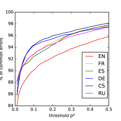
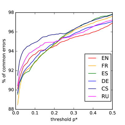
Figure 2: Percentage of errors shared by both Syl-Concat and Char-CNN on DATA-S (left) and DATA-L (right).

We see that the vast majority of errors are shared by both models even when $p^{\ast}$ is small (0.01).

PPL breakdown by token frequency: To find out how Char-CNN outperforms Syl-Concat, we partition the test sets on token frequency, as computed on the training data. We can observe in Figure 3 that, on average, the more frequent the word is, the bigger the advantage of Char-CNN over Syl-Concat. The more Char-CNN sees a word in different contexts, the more it can learn about this word (due to its powerful CNN filters). Syl-Concat, on the other hand, has limitations – it cannot see below syllables, which prevents it from extracting the same amount of knowledge about the word.

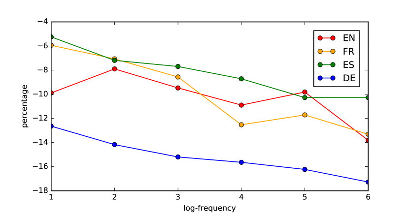
Figure 3: PPL reduction by token frequency, Char-CNN relative to Syl-Concat on DATA-L.

PCA of word embeddings: The intrinsic advantage of Char-CNN over Syl-Concat is also supported by the following experiment: We took word embeddings produced by both models on the English PTB, and applied PCA to them. Regardless of the threshold percentage of variance to retain, the embeddings from Char-CNN always have more principal components than the embeddings from Syl-Concat (see Table 4).

Model	80%	90%	95%	99%
Char-CNN	568	762	893	1038
Syl-Concat	515	729	875	1035

Table 4: Number of principle components when PCA is applied to word embeddings produced by each model, depending on % of variance to retain.

This means that Char-CNN embeds words into higher dimensional space than Syl-Concat, and thus can better distinguish them in different contexts.

LSTM limitations: During the hyperparameters tuning we noticed that increasing $d_{\mathcal{S}}$, $d_{\text{HW}}$ and $d_{\text{LM}}$ from the optimal values (in Table 2) did not result in better performance for Syl-Concat. Could it be due to the limitations of the word-level LSTM (the topmost layer in Fig. 1)? To find out whether this was the case we replaced the LSTM by a Variational RHN Zilly et al. (2017), and that resulted in a significant reduction of perplexities on PTB for both Char-CNN and Syl-Concat (Table 5). Moreover, increasing $d_{\text{LM}}$ from 439 to 650 did result in better performance for Syl-Concat. Optimization details are given in Appendix B.

Model	depth	$d_{\text{LM}}$	Size	PPL
RHN-Char-CNN	8	650	20M	67.6
RHN-Syl-Concat	8	439	13M	72.0
RHN-Syl-Concat	8	650	20M	69.4

Table 5: Replacing LSTM with Variational RHN.

Comparing syllable and morpheme embeddings: It is interesting to compare morphemes and syllables. We trained Morfessor 2.0 Creutz and Lagus (2007) in its default configuration on the PTB training data and used it instead of the syllabifier in our models. Interestingly, we got $\approx$3K unique morphemes, whereas the number of unique syllables was $\approx$6K. We then trained all our models on PTB under 5M parameter budget, keeping the state size of the word-level LSTM at 300 (as in our pre-selection step for syllable-aware models). The reduction in number of subword types allowed us to give them higher dimensionality $d_{\mathcal{M}}=100$ (cf. $d_{\mathcal{S}}=50$).

Convolutional (Morph-CNN-3) and additive (Morph-Sum) models performed better than others with test set PPLs 83.0 and 83.9 respectively. Due to limited amount of time, we did not perform a thorough hyperparameter search under 20M budget. Instead, we ran two configurations for Morph-CNN-3 and two configurations for Morph-Sum with hyperparameters close to those, which were optimal for Syl-CNN-3 and Syl-Sum correspondingly. All told, our best morpheme-aware model is Morph-Sum with $d_{\mathcal{M}}=550$, $d_{\text{HW}}=1100$, $d_{\text{LM}}=550$, and test set PPL 79.5, which is practically the same as the result of our best syllable-aware model Syl-Concat (79.4). This makes Morph-Sum a notable alternative to Char-CNN and Syl-Concat, and we defer its thorough study to future work.

Source code: The source code for the models discussed in this paper is available at https://github.com/zh3nis/lstm-syl.

7 Conclusion

It seems that syllable-aware language models fail to outperform competitive character-aware ones. However, usage of syllabification can reduce the total number of parameters and increase the training speed, albeit at the expense of language-dependent preprocessing. Morphological segmentation is a noteworthy alternative to syllabification: a simple morpheme-aware model which sums morpheme embeddings looks promising, and its study is deferred to future work.

Appendix A Pre-selection

In all models with highway layers there are two of them and the non-linear activation of any highway layer is a ReLU.

LSTM-Word: $d_{\mathcal{W}}=108$, $d_{\text{LM}}=300$.

Syl-LSTM: $d_{\mathcal{S}}=50$, $d_{\text{LM}}=300$.

Syl-CNN-[$L$]: $d_{\mathcal{S}}=50$, convolutional filter widths are $[1,\ldots,L]$, the corresponding convolutional filter depths are $[c\cdot l]_{l=1}^{L}$, $d_{\text{HW}}=c\cdot(1+\ldots+L)$. We experimented with $L=2,3,4$. The corresponding values of $c$ are chosen to be $120,60,35$ to fit the total parameter budget. CNN activation is $\tanh$.

Linear combinations: We give higher dimensionality to syllable vectors here (compared to other models) since the resulting word vector will have the same size as syllable vectors (see (3)). $d_{\mathcal{S}}=175$, $d_{\text{HW}}=175$ in all models except the Syl-Avg-B, where we have $d_{\mathcal{S}}=160$, $d_{\text{HW}}=160$.

Syl-Concat: $d_{\mathcal{S}}=50$, $d_{\text{HW}}=300$.

Appendix B Optimization

LSTM-based models: We perform the training (5) by truncated BPTT Werbos (1990); Graves (2013). We backpropagate for 70 time steps on DATA-S and for 35 time steps on DATA-L using stochastic gradient descent where the learning rate is initially set to 1.0 and halved if the perplexity does not decrease on the validation set after an epoch. We use batch sizes of 20 for DATA-S and 100 for DATA-L. We train for 50 epochs on DATA-S and for 25 epochs on DATA-L, picking the best-performing model on the validation set. Parameters of the models are randomly initialized uniformly in $[-0.05,0.05]$, except the forget bias of the word-level LSTM, which is initialized to $1$. For regularization we use dropout Srivastava et al. (2014) with probability 0.5 between word-level LSTM layers and on the hidden-to-output softmax layer. We clip the norm of the gradients (normalized by minibatch size) at 5. These choices were guided by previous work on word-level language modeling with LSTMs Zaremba et al. (2014).

To speed up training on DATA-L we use a sampled softmax Jean et al. (2015) with the number of samples equal to 20% of the vocabulary size Chen et al. (2016). Although Kim et al. (2016) used a hierarchical softmax Morin and Bengio (2005) for the same purpose, a recent study Grave et al. (2016) shows that it is outperformed by sampled softmax on the Europarl corpus, from which DATA-L was derived Botha and Blunsom (2014).

RHN-based models are optimized as in Zilly et al. (2017), except that we unrolled the networks for 70 time steps in truncated BPTT, and dropout rates were chosen to be as follows: 0.2 for the embedding layer, 0.7 for the input to the gates, 0.7 for the hidden units and 0.2 for the output activations.

Appendix C Sizes and speeds

On DATA-S, Syl-Concat has 28%–33% fewer parameters than Char-CNN, and on DATA-L the reduction is 18%–27% (see Fig. 4).

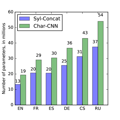
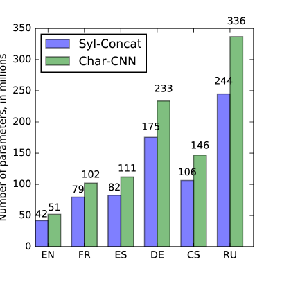
Figure 4: Model sizes on DATA-S (left) and DATA-L, in millions of trainable variables.

Training speeds are provided in the Table 6. Models were implemented in TensorFlow, and were run on NVIDIA Titan X (Pascal).

Model	EN	FR	ES	DE	CS	RU
Char-CNN	9	8	8	7	6	6	S
Syl-Concat	14	12	12	11	10	9
Char-CNN	10	8	7	5	7	4	L
Syl-Concat	22	13	13	6	10	5

Table 6: Training speeds, in thousands of tokens per second.

References

- Botha and Blunsom (2014) Jan Botha and Phil Blunsom. 2014. Compositional morphology for word representations and language modelling. In Proceedings of ICML.
- Chen et al. (2016) Wenlin Chen, David Grangier, and Michael Auli. 2016. Strategies for training large vocabulary neural language models. In Proceedings of ACL.
- Cotterell and Schütze (2015) Ryan Cotterell and Hinrich Schütze. 2015. Morphological word-embeddings. In Proceedings of HLT-NAACL.
- Creutz and Lagus (2007) Mathias Creutz and Krista Lagus. 2007. Unsupervised models for morpheme segmentation and morphology learning. ACM Transactions on Speech and Language Processing (TSLP), 4(1):3.
- Gal and Ghahramani (2016) Yarin Gal and Zoubin Ghahramani. 2016. A theoretically grounded application of dropout in recurrent neural networks. In Proceedings of NIPS.
- Grave et al. (2016) Edouard Grave, Armand Joulin, Moustapha Cissé, David Grangier, and Hervé Jégou. 2016. Efficient softmax approximation for gpus. arXiv preprint arXiv:1609.04309.
- Graves (2013) Alex Graves. 2013. Generating sequences with recurrent neural networks. arXiv preprint arXiv:1308.0850.
- Hochreiter and Schmidhuber (1997) Sepp Hochreiter and Jürgen Schmidhuber. 1997. Long short-term memory. Neural computation, 9(8):1735–1780.
- Jean et al. (2015) Sébastien Jean, Kyunghyun Cho, Roland Memisevic, and Yoshua Bengio. 2015. On using very large target vocabulary for neural machine translation. In Proceedings of ACL-IJCNLP.
- Jozefowicz et al. (2015) Rafal Jozefowicz, Wojciech Zaremba, and Ilya Sutskever. 2015. An empirical exploration of recurrent network architectures. In Proceedings of ICML.
- Kim et al. (2016) Yoon Kim, Yacine Jernite, David Sontag, and Alexander M Rush. 2016. Character-aware neural language models. In Proceedings of AAAI.
- Liang (1983) Franklin Mark Liang. 1983. Word Hy-phen-a-tion by Com-put-er. Citeseer.
- Ling et al. (2015a) Wang Ling, Lin Chu-Cheng, Yulia Tsvetkov, and Silvio Amir. 2015a. Not all contexts are created equal: Better word representations with variable attention. In Proceedings of EMNLP.
- Ling et al. (2015b) Wang Ling, Chris Dyer, Alan W Black, Isabel Trancoso, Ramon Fermandez, Silvio Amir, Luis Marujo, and Tiago Luis. 2015b. Finding function in form: Compositional character models for open vocabulary word representation. In Proceedings of EMNLP.
- Marcus et al. (1993) Mitchell P Marcus, Mary Ann Marcinkiewicz, and Beatrice Santorini. 1993. Building a large annotated corpus of english: The penn treebank. Computational linguistics, 19(2):313–330.
- Mikolov et al. (2013) Tomas Mikolov, Kai Chen, Greg Corrado, and Jeffrey Dean. 2013. Efficient estimation of word representations in vector space. arXiv preprint arXiv:1301.3781.
- Mikolov et al. (2012) Tomáš Mikolov, Ilya Sutskever, Anoop Deoras, Hai-Son Le, Stefan Kombrink, and Jan Cernocky. 2012. Subword language modeling with neural networks. preprint (http://www. fit. vutbr. cz/imikolov/rnnlm/char. pdf).
- Morin and Bengio (2005) Frederic Morin and Yoshua Bengio. 2005. Hierarchical probabilistic neural network language model. In Proceedings of AISTATS.
- Qiu et al. (2014) Siyu Qiu, Qing Cui, Jiang Bian, Bin Gao, and Tie-Yan Liu. 2014. Co-learning of word representations and morpheme representations. In Proceedings of COLING.
- Sennrich et al. (2016) Rico Sennrich, Barry Haddow, and Alexandra Birch. 2016. Neural machine translation of rare words with subword units. In Proceedings of ACL.
- Srivastava et al. (2014) Nitish Srivastava, Geoffrey E Hinton, Alex Krizhevsky, Ilya Sutskever, and Ruslan Salakhutdinov. 2014. Dropout: a simple way to prevent neural networks from overfitting. Journal of Machine Learning Research, 15(1):1929–1958.
- Srivastava et al. (2015) Rupesh K Srivastava, Klaus Greff, and Jürgen Schmidhuber. 2015. Training very deep networks. In Proceedings of NIPS.
- Vania and Lopez (2017) Clara Vania and Adam Lopez. 2017. From characters to words to in between: Do we capture morphology? In Proceedings of ACL.
- Verwimp et al. (2017) Lyan Verwimp, Joris Pelemans, Patrick Wambacq, et al. 2017. Character-word lstm language models. In Proceedings of EACL.
- Werbos (1990) Paul J Werbos. 1990. Backpropagation through time: what it does and how to do it. Proceedings of the IEEE, 78(10).
- Zaremba et al. (2014) Wojciech Zaremba, Ilya Sutskever, and Oriol Vinyals. 2014. Recurrent neural network regularization. arXiv preprint arXiv:1409.2329.
- Zilly et al. (2017) Julian Georg Zilly, Rupesh Kumar Srivastava, Jan Koutník, and Jürgen Schmidhuber. 2017. Recurrent highway networks. In Proceedings of ICML.
- Zoph and Le (2017) Barret Zoph and Quoc V Le. 2017. Neural architecture search with reinforcement learning. In Proceedings of ICLR.