Expansion of magnetic neutron stars in an energy (in)dependent spacetime

Abstract

Regarding the strong magnetic field of neutron stars and high energy regime scenario which is based on high curvature region near the compact objects, one is motivated to study magnetic neutron stars in an energy dependent spacetime. In this paper, we show that such strong magnetic field and energy dependency of spacetime have considerable effects on the properties of neutron stars. We examine the variations of maximum mass and related radius, Schwarzschild radius, average density, gravitational redshift, Kretschmann scalar and Buchdahl theorem due to magnetic field and also energy dependency of metric. First, it will be shown that the maximum mass and radius of neutron stars are increasing function of magnetic field while average density, redshift, the strength of gravity and Kretschmann scalar are decreasing functions of it. These results are due to a repulsive-like force behavior for the magnetic field. Next, the effects of the gravity’s rainbow will be studied and it will be shown that by increasing the rainbow function, the neutron stars could enjoy an expansion in their structures. Then, we obtain a new relation for the upper mass limit of a static spherical neutron star with uniform density in gravity’s rainbow (Buchdahl limit) in which such upper limit is modified as $M_{eff}<\frac{4c^{2}R}{9G}$. In addition, stability and energy conditions for the equation of state of neutron star matter are also investigated and a comparison with empirical results is done. It is notable that the numerical study in this paper is conducted by using the lowest order constrained variational (LOCV) approach in the presence of magnetic field employing AV18 potential.

I Introduction

Neutron stars with high-density baryonic matter and in the presence strong magnetic fields are of considerable interests in astrophysics. Interior strong magnetic field of a neutron star can form from the compression of constant magnetic flux. This magnetic field can be as large as $10^{19}\ G$ in the core of high density inhomogeneous gravitationally bound neutron stars Ferrer . By comparing with the observational data, the magnetic field strength of neutron stars is obtained about $10^{19}\ G$ Yuan . Besides, in the quark core of the high density neutron stars, the maximum field may reach up to about $10^{20}\ G$ Ferrer ; Tatsumi . On the other hand, in order to study the compact objects such as neutron and quark stars, one has to consider the effects of their curvature in the context of general relativity (GR). The first hydrostatic equilibrium equation (HEE) for stars was obtained by Tolman, Oppenheimer, and Volkoff (TOV) TolmanI ; TolmanII ; Oppenheimer . Employing TOV equation for investigating the properties of compact objects has been done by many authors Silbar ; Narain ; BordbarBY ; BoonsermVW ; LiX ; Oliveira ; He ; Yunes .

Strong magnetic fields have important influences on the structure of compact objects Heyl ; Cardall ; Kiuchi ; Ciolfi ; Lopes ; Chirenti ; Cheoun ; Belvedere ; Neilsen ; LopesDM . Using magnetohydrodynamic simulation in full GR, the stability of neutron stars with toroidal magnetic fields has been studied Kiuchi . It is found that non-rotating neutron stars are dynamically unstable for some value of magnetic field strength. Considering the equation of state (EoS) of the nuclear matter within a relativistic model subjected to a strong magnetic field, it has been shown that, the influence of magnetic field can increase the mass by more than $10\%$ for stars with hyperons interior Lopes . Employing an effective field theory model for the nuclear EoS and by considering two magnetic field geometries (tangled field and a force-free field), Kamiab et al Kamiab have shown that these fields have specific effects on the mass of neutron stars, so that it leads to increasing of the maximum mass more that $30\%$. The effects of a strong magnetic field on the nuclear EoS has been studied in Broderick . Cardall et al. Cardall have investigated static neutron stars by considering polodal magnetic fields with a simple class of electric current distribution. They have used the nuclear EoS evaluated by Broderick et al. in Ref. Broderick , and found that the magnetic field increases the maximum mass of neutron stars, Astashenok et al. Astashenok studied neutron stars in the context of F(R) gravity. They have used a nuclear EoS which was similar to the one extracted by Broderick et al. Broderick , and by assuming the global effect of magnetic field pressure, they found that the magnetic field can also increase the maximum mass of neutron star. The effects of strong magnetic fields on the structure of neutron stars in a perturbative $F(R)$ gravity and also a quantum hydrodynamics model have been investigated in Cheoun . It is shown that there exists a set of parameters for the modified gravity and magnetic field strength in which even a soft EoS can accommodate a large maximum neutron star mass through the modified mass-radius relation. In the framework of GR and relativistic mean field theory, employing the coupled Einstein-Maxwell-Thomas-Fermi equations, a model for both static and uniformly rotating neutron stars has been developed Belvedere . It is believed that the use of realistic parameters of rotating neutron stars obtained from numerical integration of the self-consistent axisymmetric general relativistic equations of equilibrium leads to the values of magnetic field and radiation efficiency of pulsars very different from estimates based on fiducial parameters.

In solar system scale or other moderate gravitational regimes, GR is an effective theory with accurate results, whereas in context of strong gravity (near the compact objects), this theory has problems various in which we address some of them. From the cosmological point of view, the usual GR cannot explain the accelerating expansion of the universe PerlmutterI ; PerlmutterII ; Riess . On the other hand, in order to construct a quantum theory of gravity, we have to evaluate the validity of theory in the ultraviolet (UV) regime. It was shown that GR is valid in infrared (IR) limit while in UV regime, it needs to improve for producing accurate results. Therefore, in order to include the UV regime, we have to modify GR. Horava-Lifshitz gravity Horava and gravity’s rainbow MagueijoII are two theories which include the UV regime by considering a modification of the usual energy-momentum relation. Among these two theories, gravity’s rainbow has more interesting results. Garattini and Saridakis GarattiniSar have shown that considering a suitable choice of the rainbow functions, the Horava-Lifshitz gravity can be related to the gravity’s rainbow.

Gravity’s rainbow can be originate from the generalization of double special relativity to the curved spacetime. The doubly special relativity Amelino-Camelia is the special relativity when we consider another upper limit constant to this theory. Indeed, in doubly special relativity there are two fundamental constants; the velocity of light ($c$), and the Planck energy ($E_{p}$). In doubly special relativity, a particle can not attain velocity and energy larger than $c$ and $E_{p}$, respectively ($v<c$ and $E<E_{p}$, in which $v$ and $E$ are, respectively, the velocity and the energy of a test particle). In this theory, the metric specifying spacetime is constructed by employing the spectrum of energy that particles can obtain Peng . Generalization of doubly special relativity in the presence of gravity leads to double GR or gravity’s rainbow MagueijoII . It is notable that, the gravity’s rainbow reduces to GR in the IR limit, in which the energy of particles has no direct effect on the curvature.

It was pointed out that although gravity’s rainbow modifies thermodynamical aspects of the black objects Ali ; HendiFEP ; HendiPEM , the uncertainty principle is valid LingLZ ; LiH . The effects of this gravity on information paradox posed by Hawking radiation and black holes evaporation have been studied in Ref. AliFM . Also, this theory has been investigated in context of black holes with different configurations Galan ; Gim . Another interesting result of this gravity is related to early universe. Indeed by considering the energy dependent Friedmann-Robertson-Walker metric, one can study the early universe without big bang singularity NonsingularI ; NonsingularII ; NonsingularIII ; NonsingularIV . Therefore, it is important to investigate the structure of other compact objects such as neutron and quark stars in this theory.

In the present work, firstly, we want to study the effects of strong magnetic field on the structure of neutron star in Einstein gravity. Then, by generalizing Einstein gravity to gravity’s rainbow in the present of strong magnetic fields, we will simultaneously investigated the effects of these two factors (magnetic field and rainbow function) on the structure of neutron star matter.

II Structure properties of magnetized neutron stars

In this paper, we are going to investigate the properties of the magnetized neutron stars using the TOV equation and the EoS introduced in Appendix (see Fig. 7 in Appendix B). The TOV equation in Einstein gravity is given by TolmanI ; TolmanII ; Oppenheimer

$$\frac{dP}{dr}=\frac{G\left(c^{2}M+4\pi r^{3}P\right)}{c^{2}r\left(2GM-c^{2}r\right)}\left(c^{2}\rho+P\right),$$ (1)

where $M=\int 4\pi r^{2}\rho(r)dr$, also $P$ and $\rho$ are, respectively, the pressure and density of the fluid which are measured by local observer. $G$ in the above equation is the gravitational constant.

Selecting central density under the boundary conditions $P(0)=P_{c}$, $m(0)=0$, we integrate the TOV equation outwards to radius $r=R$, at which $P$ vanishes. This yields the radius $R$ and mass $M=m(R)$ (see Ref. Shapiro ). The effects of magnetic field on the gravitational mass and radius of neutron star are presented in table 1. Also, the effects of magnetic field on the diagrams related to mass-central mass density ($M-\rho$) and mass-radius ($M-R$) relations are presented in Fig. 1. We found that the maximum mass and radius of magnetized neutron stars increase when the magnetic field grows. In order to more investigation the effect of magnetic field on neutron star, we study other interesting properties of our solution.

One of interesting quantities of neutron star is related to the average density of the magnetized neutron star can be written as

$$\overline{\rho}=\frac{3M}{4\pi R^{3}},$$ (2)

the obtained results of average density for different magnetic fields are interesting. According to table 1 one finds that the average density decreases when magnetic field increases. In other words, growing magnetic field, unlike gravitational attraction, leads to more expansions of neutron stars.

Another important quantity which is related to the compactness of a spherical object. It can be defined as the ratio of the Schwarzschild radius to the radius of object,

$$\sigma=\frac{R_{Sch}}{R},$$ (3)

which may be interpreted as the strength of gravity. Also the Schwarzschild radius is $R_{Sch}=\frac{2GM}{c^{2}}$. Another quantity which shows the strength of gravity is related to the spacetime curvature. In Schwarzschild metric, the components of Ricci tensor ($R_{\mu\nu}$) and the Ricci scalar ($R$) are zero outside the star and these quantities do not give us any information about the spacetime curvature. Therefore, we use another quantity in order to more investigation of the curvature of spacetime. The quantity which can help us to understand the curvature of spacetime is the Riemann tensor. According to this fact the Riemann tensor may have more components and for simplicity we can study the Kretschmann scalar for measuring of the curvature in vacuum. Therefore, the curvature at the surface of a neutron star in Einstein gravity is given as Psaltis ; Eksi

$$K=\sqrt{R_{\mu\nu\alpha\beta}R^{\mu\nu\alpha\beta}}=\frac{4\sqrt{3}GM}{c^{2}R^{3}},$$ (4)

The numerical results confirm that by increasing the magnetic field, the strength of gravity decreases and this may increase the radius of these stars.

Another known parameter of neutron stars is the gravitational redshift which can be written in the following form

$$z=\frac{1}{\sqrt{1-\frac{2GM}{c^{2}R}}}-1,$$ (5)

as one can see, increasing $B$, leads to decreasing the redshift.

The dynamical stability of the stellar model against the infinitesimal radial adiabatic perturbation was introduced by Chandrasekhar Chandrasekhar . This stability condition was developed and applied to astrophysical cases by many authors BardeenTM ; Kuntsem ; Mak ; Kalam . The dynamical stability condition is satisfied when the adiabatic index, $\gamma$, is larger than $\frac{4}{3}$, i.e, $\gamma>\frac{4}{3}=1.33$, everywhere within the isotropic star. The adiabatic index is defined in the following form

$$\gamma=\frac{\rho c^{2}+P}{c^{2}P}\frac{dP}{d\rho}.$$ (6)

In order to investigate the dynamical stability of magnetized neutron star, we plot the adiabatic index versus the radius in Fig. 2. As one can see, these stars enjoy interior dynamical stability.

Table 1: Properties of neutron star with different magnetic fields.

$B(G)$	${M_{max}}\ (M_{\odot})$	$R\ (km)$	$R_{Sch}\ (km)$	$\overline{\rho}$ $(10^{15}g$ $cm^{-3})$	$\sigma(\frac{R_{Sch}}{R})$	$z$	$K(10^{-7}$ $m^{-2})$	$\frac{4c^{2}R}{9G}\ (M_{\odot})$
$0$	$1.68$	$8.42$	$4.95$	$1.34$	$0.59$	$0.56$	$0.29$	$2.54$
$5\times 10^{18}$	$1.70$	$8.88$	$5.01$	$1.15$	$0.56$	$0.51$	$0.25$	$2.68$
$1\times 10^{19}$	$1.71$	$9.36$	$5.04$	$0.99$	$0.54$	$0.47$	$0.21$	$2.82$

$\begin{array}[]{cc}\epsfbox{MverdenB0.eps}&\epsfbox{MverrB0.eps}\end{array}$

Figure 1: Gravitational mass versus the density $(10^{15}g$ $cm^{-3})$ (right diagram) and radius (left diagram), for $B=0$ (doted line), $B=5\times 10^{18}G$ (continuous line), and $B=1\times 10^{19}G$ (dashed line).

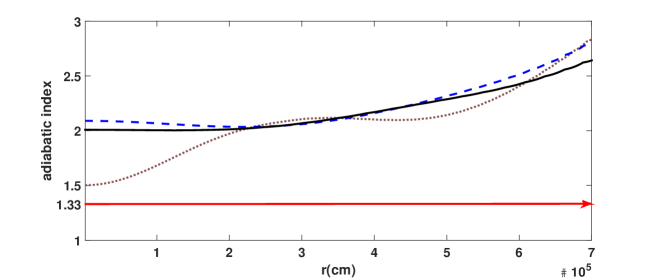
Figure 2: The adiabatic index versus the radius for $B=0$ (doted line), $B=5\times 10^{18}G$ (dashed line), and $B=1\times 10^{19}G$ (continuous line).

Here, we want to investigate the upper mass limit of a static spherical neutron star with uniform density in GR, so-called Buchdahl theorem Buchdahl . The GR compactness limit is given by Buchdahl

$$M\leq\frac{4c^{2}R}{9G},$$ (7)

in which the upper mass limit is $M_{\max}=\frac{4c^{2}R}{9G}$. Our numerical results confirm that the obtained mass of magnetic neutron stars in GR respects Eq. (7).

Studying Fig. 7 (Appendix B), shows that the core of neutron star is more rigid when the magnetic field increases, whiles the radius of magnetic neutron star is an increasing function of magnetic field, but the average density, compactness, redshift and Kretschmann scalar are decreasing functions of it. Therefore, by increasing the magnetic field, although core of the neutron star remains compact, the outer layers expand. As a results, the magnetic field has repulsive property.

Theoretically, it has been shown that the magnetic field contributes directly to the pressure in the Einstein equations in which pressure fits with square magnetic field ($P_{B}\propto B^{2}$) , see Refs. LopesDM ; Astashenok ; Moradi:2017alp ; Ray:2003gt for more details. This shows that when magnetic field is increased, associated magnetic pressure, due to its repulsive nature, increases the radius of neutron star. In other words, by adding the magnetic field to our system, its pressure increases. Such increasing in the pressure leads to increasing the repulsive force and as a result the system will be unstable. In order to have a stable case, the mass of the neutron star must increase. Therefore, it is a direct effect that when magnetic field is increased, the total mass of system is increased, too.

In the next section, we want to evaluate the effects of gravity’s rainbow on the structure of neutron stars.

III Structure properties of neutron stars in gravity’s rainbow

Here we introduce the spherical symmetric metric in gravity’s rainbow as

$$ds^{2}=-\frac{\Psi(r)}{F^{2}(\varepsilon)}dt^{2}+\frac{dr^{2}}{H^{2}(\varepsilon)\Psi(r)}+r^{2}\left(d\theta^{2}+\sin^{2}(\theta)d\varphi^{2}\right),$$ (8)

in which $H(\varepsilon)$ and $F(\varepsilon)$ are rainbow functions. In order to study the structure of neutron stars in gravity’s rainbow, firstly we should obtain the HEE in this gravity. The HEE in gravity’s rainbow by considering the metric (8) and the following field equation

$$G_{\mu}^{\nu}=\frac{8\pi G}{c^{4}}T_{\mu}^{\nu},$$ (9)

where $G_{\mu}^{\nu}$ and $T_{\mu}^{\nu}$ are the Einstein and energy-momentum tensors, respectively, is given by HendiBEP

$$\frac{dP}{dr}=\frac{G\left(c^{2}M_{eff}H^{2}(\varepsilon)+4\pi r^{3}P\right)}{c^{2}r\left(2GM_{eff}-c^{2}r\right)H^{2}(\varepsilon)}\left(c^{2}\rho+P\right),$$ (10)

where

$$M_{eff}\left(r,\varepsilon\right)=\int\frac{4\pi}{H^{2}(\varepsilon)}r^{2}\rho(r)dr.$$ (11)

Here, we consider an upper limit for energies which $\varepsilon\leq 1$ ($\varepsilon=\frac{E}{E_{p}}$, which $E$ and $E_{P}$ are particle and Planck energies, respectively. See Refs. MagueijoII ; GarattiniSar ; Amelino-Camelia ; Peng ; Ali ; HendiFEP ; HendiPEM for more details). For $H(\varepsilon)=1$, the equation (10) yields to the usual TOV equation TolmanI ; TolmanII ; Oppenheimer (see Eq. (1)).

It is notable that there are known three cases for the rainbow function. The first one is related to the hard spectra from gamma-ray bursts AmelinoNature , with the following form

$$F\left(\varepsilon\right)=\frac{e^{\beta\varepsilon}-1}{\beta\varepsilon},~{}~{}~{}~{}\&~{}~{}~{}~{}H\left(\varepsilon\right)=1.$$ (12)

The second one is motivated by studies conducted in loop quantum gravity and non-commutative geometry Jacob ; AmelinoLRR as

$$F\left(\varepsilon\right)=1,~{}~{}~{}~{}\&~{}~{}~{}~{}H\left(\varepsilon\right)=\sqrt{1-\eta\varepsilon^{n}}.$$ (13)

The third one of energy function is due to the consideration of constancy of the velocity of light MagueijoI

$$F\left(\varepsilon\right)=H\left(\varepsilon\right)=\frac{1}{1-\lambda\varepsilon},$$ (14)

where in the above models $\beta$, $\eta$ and $\lambda$ are constants which can be adjusted by experiment. Here, we are going to investigate more properties of the neutron stars by using the obtained HEE in gravity’s rainbow. As it was shown, the obtained HEE for gravity’s rainbow only depends to rainbow function of $H\left(\varepsilon\right)$. This shows that, the first model can not be useful for investigating the structure of neutron stars, because in this case the extracted HEE will yield Einstein’s HEE (TOV equation) and we do not see any effects of rainbow functions. We consider the third model for three reasons; i) more effectiveness; this model (third model) affects temporal and spatial coordinates, simultaneously, on the contrary, the effects of the first and second models are only on temporal coordinate and spatial coordinates, respectively. ii) low number of free parameters; there are two free parameters for the second model, whereas the third model has one free parameter. iii) phenomenologically logical; third set of rainbow functions comes from the constancy of light velocity, which we would like to respect it. The results are collected in table 2. As one can see, by increasing rainbow function, the maximum mass and the corresponding radius of neutron star increase. This emphasizes the contributions of the gravity’s rainbow on properties of neutron stars.

The average density of neutron star in this gravity can be written as

$$\overline{\rho}=\frac{3M_{eff}}{4\pi R^{3}}.$$ (15)

Table 2 shows that the average density decreases when $H(\varepsilon)$ increases. The Schwarzschild radius in this gravity is given as HendiBEP

$$R_{Sch}=\frac{2GM_{eff}}{c^{2}},$$ (16)

the Schwarzschild radius increases when $H(\varepsilon)$ increases.

We obtain the compactness of a spherical object ($\sigma$), by using the obtained Schwarzschild radius (Eq. (16)) and Eqs. (3) and (11), as

$$\sigma=\frac{8\pi G}{c^{2}H^{2}(\varepsilon)R}\int_{0}^{R}r^{2}\rho\left(r\right)dr.$$ (17)

The gravitational redshift in gravity’s rainbow can be written in the following form HendiBEP

$$z=\frac{1}{\sqrt{1-\frac{2GM_{eff}}{c^{2}R}}}-1=\frac{1}{\sqrt{1-\frac{8\pi G}{c^{2}H^{2}\left(\varepsilon\right)R}\int_{0}^{R}r^{2}\rho\left(r\right)dr}}-1=\frac{1}{\sqrt{1-\sigma}}-1.$$ (18)

The above equations show that the compactness of a spherical object and the gravitational redshift depend on both the rainbow function ($H^{2}\left(\varepsilon\right)$) and the radius of neutron star ($R$). On the other hand, numerical calculations showed that increasing the rainbow function leads to increasing the radius of neutron star, too. So, based on numerical calculations, we have concluded that changing the rainbow function does not have any significant role in $\sigma$ and $z$ up to our numeric precision (see table. 2). Also, it was shown that, these stars have the dynamical stability (see Figs. 5 and 6 of Ref. HendiBEP , for more details).

Table 2: Structure properties of neutron star in gravity’s rainbow with $F(\varepsilon)=H(\varepsilon)=\frac{1}{1-\lambda\varepsilon}$ for $\lambda=2$.

$E(E_{pl})$	$H(\varepsilon)$	${M_{max}}\ (M_{\odot})$	$R\ (km)$	$R_{Sch}\ (km)$	$\overline{\rho}$ $(10^{15}g$ $cm^{-3})$	$\sigma(\frac{R_{Sch}}{R})$	$z$	$K(10^{-7}$ $m^{-2})$	$\frac{4c^{2}R}{9G}\ (M_{\odot})$
$E\ll 1$	$1.00$	$1.68$	$8.42$	$4.95$	$1.34$	$0.59$	$0.56$	$0.29$	$2.54$
$0.0833$	$1.20$	$2.02$	$10.10$	$5.95$	$0.93$	$0.59$	$0.56$	$0.25$	$3.04$
$0.1428$	$1.40$	$2.36$	$11.79$	$6.99$	$0.69$	$0.59$	$0.56$	$0.24$	$3.55$
$0.1875$	$1.60$	$2.69$	$13.47$	$7.93$	$0.52$	$0.59$	$0.56$	$0.24$	$4.06$
$0.2222$	$1.80$	$3.03$	$15.16$	$8.93$	$0.41$	$0.59$	$0.56$	$0.24$	$4.57$
$0.2500$	$2.00$	$3.37$	$16.84$	$9.93$	$0.34$	$0.59$	$0.56$	$0.24$	$5.08$

Here we want to obtain the curvature at the surface of a neutron star in gravity’s rainbow. Considering the metric (8) with field equation (9), we can obtain the Kretschmann scalar as 

$$K=\frac{2H(\varepsilon)}{R^{2}}\sqrt{\left[1-\frac{4GM\left(c^{2}R-3GM\right)}{c^{4}R^{2}}\right]H^{4}(\varepsilon)+\frac{2\left(2GM-c^{2}R\right)H^{2}(\varepsilon)}{c^{2}R}+1}.$$ (19)

It is notable that when $H(\varepsilon)=1$, the Kretschmann scalar of Einstein gravity (Eq. 4) will be recovered. The results show that, by increasing rainbow function which leads to increasing of radius and mass of neutron stars, but the strength of gravity decreases.

Another important quantity which is interesting for evaluation is related to the upper mass limit of a static spherical neutron star with uniform density in gravity’s rainbow. For this purpose, we have to obtain Buchdahl theorem in an energy dependent spacetime. Solving the integral given in Eq. (11), we obtain

$$M_{eff}=\frac{4\pi\rho}{3H^{2}(\varepsilon)}r^{3}.$$ (20)

Inserting Eq. (20) into the obtained HEE in gravity’s rainbow (10), we have

$$\frac{dP}{dr}=-\frac{4\pi Gr}{3c^{4}H^{2}(\varepsilon)}\frac{\left(c^{2}\rho+3P\right)\left(c^{2}\rho+P\right)}{\left(1-\frac{8\pi G}{3c^{2}H^{2}(\varepsilon)}\rho r^{2}\right)}.$$ (21)

Integrating from a central pressure $p_{c}=p(r=0)$, we have

$$\int_{p_{c}}^{p}\frac{dP^{\prime}}{\left(c^{2}\rho+3P^{\prime}\right)\left(c^{2}\rho+P^{\prime}\right)}=-\frac{4\pi G}{3c^{4}H^{2}(\varepsilon)}\int_{0}^{r}\frac{r^{\prime}dr^{\prime}}{\left(1-\frac{8\pi G}{3c^{2}H^{2}(\varepsilon)}\rho r^{\prime 2}\right)},$$ (22)

in which the integral on the right-hand side of the above equation is

$$-\frac{4\pi G}{3c^{4}H^{2}(\varepsilon)}\int_{0}^{r}\frac{r^{\prime}dr^{\prime}}{\left(1-\frac{8\pi G}{3c^{2}H^{2}(\varepsilon)}\rho r^{\prime 2}\right)}=\frac{1}{4c^{2}\rho}\int_{1}^{1-\frac{8\pi G}{3c^{2}H^{2}(\varepsilon)}\rho r^{2}}\frac{dy}{y}=\frac{1}{4c^{2}\rho}\ln y\left|{}_{1}^{1-\frac{8\pi G}{3c^{2}H^{2}(\varepsilon)}\rho r^{2}}\right.$$

$$=\frac{1}{4c^{2}\rho}\ln\left(1-\frac{8\pi G}{3c^{2}H^{2}(\varepsilon)}\rho r^{2}\right),$$ (23)

which we have used of $y=1-\frac{8\pi G}{3H^{2}(\varepsilon)}r^{\prime 2}\rho$ in the above equation. On the other hand, the left-hand side of Eq. (22) is

$$\int_{p_{c}}^{p}\frac{dP^{\prime}}{\left(c^{2}\rho+3P^{\prime}\right)\left(c^{2}\rho+P^{\prime}\right)}=\frac{1}{2c^{2}\rho}\left.\ln\left(\frac{c^{2}\rho+3P^{\prime}}{c^{2}\rho+P^{\prime}}\right)\right|_{p_{c}}^{p}$$

$$=\frac{1}{2c^{2}\rho}\left[\ln\left(\frac{c^{2}\rho+3P}{c^{2}\rho+P}\right)-\ln\left(\frac{c^{2}\rho+3P_{c}}{c^{2}\rho+P_{c}}\right)\right].$$ (24)

Combining Eqs. (23) and (24), we can write

$$\frac{1}{2c^{2}\rho}\left[\ln\left(\frac{c^{2}\rho+3P}{c^{2}\rho+P}\right)-\ln\left(\frac{c^{2}\rho+3P_{c}}{c^{2}\rho+P_{c}}\right)\right]=\frac{1}{4c^{2}\rho}\ln\left(1-\frac{8\pi G}{3c^{2}H^{2}(\varepsilon)}\rho r^{2}\right),$$ (25)

so we have

$$\frac{c^{2}\rho+3P}{c^{2}\rho+P}=\frac{c^{2}\rho+3P_{c}}{c^{2}\rho+P_{c}}\sqrt{1-\frac{8\pi G}{3c^{2}H^{2}(\varepsilon)}\rho r^{2}},$$ (26)

in which by using Eq. (20), we can rewrite it as

$$\frac{c^{2}\rho+3P}{c^{2}\rho+P}=\frac{c^{2}\rho+3P_{c}}{c^{2}\rho+P_{c}}\sqrt{1-\frac{2GM_{eff}\left(r,\varepsilon\right)}{c^{2}r}}.$$ (27)

In order to obtain an expression for finding how the radius of star depends on its mass and density, we use the fact that the pressure of a star on its surface vanishes, i.e., $p(r)=0$ for $r=R$ ($p(R)=0$). So we can obtain

$$\frac{2GM_{eff}}{c^{2}R}=1-\left(\frac{c^{2}\rho+P_{c}}{c^{2}\rho+3P_{c}}\right)^{2}.$$ (28)

Introducing a new dimensionless variable as $x=\frac{c^{2}\rho}{P_{c}}$ , we can rewrite Eq. (28) with the following form

$$\frac{2GM_{eff}}{c^{2}R}=1-\left(\frac{x+1}{x+3}\right)^{2}=1-\left[S(x)\right]^{2},$$ (29)

where $S(x)=\frac{x+1}{x+3}$. According to this fact the variable $x$ is functions of $P_{c}$ and $\rho$ in which both them can never be negative, hence $x$ can not be negative and also due to the negative sign of the $S(x)$, Eq. (29) reaches its maximum value when $S(x)$ reaches its minimum  value. In order to find the minimum of the $S(x)$, we find the derivative as $\frac{dS(x)}{dx}=\frac{2}{\left(x+3\right)^{2}}$. This is always positive. Thus $S(x)$ increases with increasing $x$, and the minimum of $S(x)$ is located at $x=0$. Inserting $x=0$ in Eq. (29), we have

$$\frac{GM_{eff\max}}{c^{2}R}=\frac{4}{9},~{}~{}~{}~{}or~{}~{}~{}~{}~{}M_{eff\max}=\frac{4c^{2}R}{9G}.$$ (30)

The equation (30) gives the value for the maximum mass of a star of given radius in gravity’s rainbow. As a results of our calculation for finding the upper mass limit for a static spherical neutron star with uniform density in gravity’s rainbow, the obtained mass of neutron stars we must be in the range

$$M_{eff}<\frac{4c^{2}R}{9G}.$$ (31)

It is notable that, for $H(\varepsilon)=1$, this limit reduces to Einstein case ($M<\frac{4c^{2}R}{9G}$). Our results of mass of magnetic neutron stars in gravity’s rainbow show that these masses are in the obtained range of Eq. (31).

The maximum mass and radius of neutron star are increasing functions of the rainbow function while the average density and the Kretschmann scalar were a decreasing function of it. These properties indicate that increasing the rainbow function results into expansion of the neuron star.

IV Structure properties of magnetized neutron stars in gravity’s rainbow

Considering the EoS introduced in Appendix A and B, we want to calculate the properties of magnetic neutron star in gravity’s rainbow in this section. The effects of rainbow function and magnetic field on the diagrams related to $M-\rho$ and $M-R$ relations are presented in Figs. 3 and 4. As one can see, by increasing rainbow function and magnetic field, the maximum mass and radius of magnetized neutron stars increase. It is notable that for $H(\varepsilon)=1$, the maximum mass of these stars reduces to the results obtained in the Einstein gravity (see table 1), as expected. By increasing rainbow function ($H(\varepsilon)>1$) and magnetic field, the maximum mass of these stars will be larger than the case of the Einstein gravity (see table 3 and Figs. 3 and 4). This emphasizes the contributions of the gravity’s rainbow and magnetic field on properties of neutron stars. The effects of magnetic fields on the gravitational masses of neutron stars and M-R relation for a fixed amount of the rainbow function are presented in Fig. 5. The maximum mass and radius of magnetized neutron star for each value of the rainbow function increase when the magnetic field grows (see table 3). Our results cover the mass measurement of massive magnetized neutron stars. For example; about $1.8M_{\odot}$ for Vela X-1 Rawlset , PSR J1614-2230 Demorest about $1.97M_{\odot}$, PSR J0348+0432 Antoniadis about $2.01M_{\odot}$, 4U 1700-377 Clark et al about $2.4M_{\odot}$, and J1748-2021B Freire about $2.7M_{\odot}$.

Previously, Rhoades and Ruffini have shown that by employing the principles of causality and Le Chantelier in Einstein gravity, the mass of neutron star can not be larger than $3.2M_{\odot}$ Ruffini . Here, it was shown that the principles of causality and Le Chantelier are valid for the EoS in this paper (see Appendix B). In addition, we find that depending on choices of rainbow function, the mass of the neutron star could be larger than $3.2M_{\odot}$.

The results for the Schwarzschild radius show that for each value of the magnetic field with stronger gravity’s rainbow, the Schwarzschild radius has higher value. In addition, with a fixed amount of rainbow function, the Schwarzschild radius grows when the magnetic field increases. Moreover, the average density of the magnetized neutron star shows that the average density decreases when both $H(\varepsilon)$ and $B$ increase.

The compactness of this star confirms when $H(\varepsilon)$ increases, the strength of gravity is the same, but by increasing the magnetic field, the strength of gravity decreases and this may increase the radius of this star.

Using Eq. (19), we find that for a fixed value of the magnetic field by increasing rainbow function, the strength of gravity of a neutron star has smaller values. In addition, with a fixed amount of rainbow function, the Kretschmann scalar decreases when the magnetic field increases.

It is notable that, by increasing $B$ leads to decreasing the gravitational redshift. On the other hand, considering a fixed value of magnetic field, the rainbow function does not affect the gravitational redshift. Our results show that, the maximum redshift for this star is about $0.51$, which is lower than the upper bound on the surface redshift for a subluminal equation of state, i.e $z=0.85$ HaeselII .

In order to investigate the dynamical stability of magnetized neutron star, we plot the adiabatic index versus the radius in Fig. 6. As one can see, these stars have the dynamical stability inside.

Table 3: Properties of magnetic neutron star in gravity’s rainbow with $F(\varepsilon)=H(\varepsilon)=\frac{1}{1-\lambda\varepsilon}$ for $\lambda=2$.

$E(E_{pl})$	$H(\varepsilon)$	$B(G)$	${M_{max}}\ (M_{\odot})$	$R\ (km)$	$R_{Sch}\ (km)$	$\overline{\rho}$ $(10^{15}g$ $cm^{-3})$	$\sigma(\frac{R_{Sch}}{R})$	$z$	$K(10^{-7}$ $m^{-2})$	$\frac{4c^{2}R}{9G}\ (M_{\odot})$
$E\ll 1$	$1.00$	$\begin{array}[]{c}5\times 10^{18}\\ 1\times 10^{19}\end{array}$	$\begin{array}[]{c}1.70\\ 1.71\end{array}$	$\begin{array}[]{c}8.88\\ 9.36\end{array}$	$\begin{array}[]{c}5.01\\ 5.04\end{array}$	$\begin{array}[]{c}1.15\\ 0.99\end{array}$	$\begin{array}[]{c}0.56\\ 0.54\end{array}$	$\begin{array}[]{c}0.51\\ 0.47\end{array}$	$\begin{array}[]{c}0.25\\ 0.21\end{array}$	$\begin{array}[]{c}2.68\\ 2.82\end{array}$
$0.0833$	$1.20$	$\begin{array}[]{c}5\times 10^{18}\\ 1\times 10^{19}\end{array}$	$\begin{array}[]{c}2.03\\ 2.05\end{array}$	$\begin{array}[]{c}10.66\\ 11.23\end{array}$	$\begin{array}[]{c}5.98\\ 6.04\end{array}$	$\begin{array}[]{c}0.79\\ 0.69\end{array}$	$\begin{array}[]{c}0.56\\ 0.54\end{array}$	$\begin{array}[]{c}0.51\\ 0.47\end{array}$	$\begin{array}[]{c}0.21\\ 0.18\end{array}$	$\begin{array}[]{c}3.21\\ 3.38\end{array}$
$0.1428$	$1.40$	$\begin{array}[]{c}5\times 10^{18}\\ 1\times 10^{19}\end{array}$	$\begin{array}[]{c}2.37\\ 2.40\end{array}$	$\begin{array}[]{c}12.43\\ 13.10\end{array}$	$\begin{array}[]{c}6.99\\ 7.07\end{array}$	$\begin{array}[]{c}0.58\\ 0.51\end{array}$	$\begin{array}[]{c}0.56\\ 0.54\end{array}$	$\begin{array}[]{c}0.51\\ 0.47\end{array}$	$\begin{array}[]{c}0.20\\ 0.18\end{array}$	$\begin{array}[]{c}3.75\\ 3.95\end{array}$
$0.1875$	$1.60$	$\begin{array}[]{c}5\times 10^{18}\\ 1\times 10^{19}\end{array}$	$\begin{array}[]{c}2.71\\ 2.74\end{array}$	$\begin{array}[]{c}14.21\\ 14.98\end{array}$	$\begin{array}[]{c}7.99\\ 8.08\end{array}$	$\begin{array}[]{c}0.45\\ 0.39\end{array}$	$\begin{array}[]{c}0.56\\ 0.54\end{array}$	$\begin{array}[]{c}0.51\\ 0.47\end{array}$	$\begin{array}[]{c}0.20\\ 0.18\end{array}$	$\begin{array}[]{c}4.28\\ 4.52\end{array}$
$0.2222$	$1.80$	$\begin{array}[]{c}5\times 10^{18}\\ 1\times 10^{19}\end{array}$	$\begin{array}[]{c}3.05\\ 3.08\end{array}$	$\begin{array}[]{c}16.10\\ 16.84\end{array}$	$\begin{array}[]{c}8.99\\ 9.08\end{array}$	$\begin{array}[]{c}0.35\\ 0.31\end{array}$	$\begin{array}[]{c}0.56\\ 0.54\end{array}$	$\begin{array}[]{c}0.51\\ 0.47\end{array}$	$\begin{array}[]{c}0.20\\ 0.18\end{array}$	$\begin{array}[]{c}4.85\\ 5.08\end{array}$
$0.2500$	$2.00$	$\begin{array}[]{c}5\times 10^{18}\\ 1\times 10^{19}\end{array}$	$\begin{array}[]{c}3.39\\ 3.42\end{array}$	$\begin{array}[]{c}17.76\\ 18.72\end{array}$	$\begin{array}[]{c}9.99\\ 10.08\end{array}$	$\begin{array}[]{c}0.29\\ 0.25\end{array}$	$\begin{array}[]{c}0.56\\ 0.54\end{array}$	$\begin{array}[]{c}0.51\\ 0.47\end{array}$	$\begin{array}[]{c}0.20\\ 0.18\end{array}$	$\begin{array}[]{c}5.35\\ 5.64\end{array}$

$\begin{array}[]{cc}\epsfbox{MverdenB2.eps}&\epsfbox{MverrB2.eps}\end{array}$

Figure 3: Gravitational mass versus the density $(10^{15}g$ $cm^{-3})$ (right diagram) and radius (left diagram), for $B=5\times 10^{18}G$, $H(\varepsilon)=0.9$ (continuous line), $H(\varepsilon)=1$ (doted line), $H(\varepsilon)=1.2$ (dashed line), $H(\varepsilon)=1.5$ (dashed-dotted line), and $H(\varepsilon)=1.7$ (bold line).

$\begin{array}[]{cc}\epsfbox{MverdenB3.eps}&\epsfbox{MverrB3.eps}\end{array}$

Figure 4: Same as Figs. 3 but for $B=1\times 10^{19}G$.

$\begin{array}[]{cc}\epsfbox{MverdenB.eps}&\epsfbox{MverrB.eps}\end{array}$

Figure 5: Gravitational mass versus the density $(10^{15}g$ $cm^{-3})$ (right diagram) and radius (left diagram), for $H(\varepsilon)=1.2$, $B=0$ (continuous line), $B=5\times 10^{18}G$ (doted line), and $B=1\times 10^{19}G$ (dashed line).

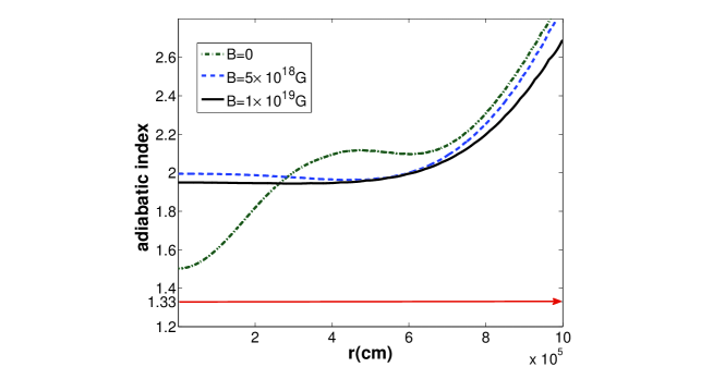
Figure 6: The adiabatic index versus the radius for $H(\varepsilon)=1.4$.

As previously mentioned, the pressure can be written as $P_{B}\propto B^{2}$. In other words, by adding the magnetic pressure ($P_{B}$) to the pressure of the fluid ($P$), the pressure power increases. On the other hand, in order to have a stable magnetic neutron star, the gravitational force has to increase and this leads to increasing of mass of magnetic neutron star.

V Comparison between theory and observations

One of the interesting features of our calculations is related to comparison of the theory and its predictions with the empirical evidences. For this purpose, we compare our results with the observational data. We have presented this comparison in table 4. It is clear that the results derived in this theory are in agreement with the results obtained through observations. It is notable that for non-magnetized neutron stars, the radius obtained through gravity’s rainbow are smaller than the observed values. However, the radius of the magnetized neutron stars are in the range of the observed values. This is due to the fact that we have considered the magnetic field of neutron stars in our calculations (see table 4 for more details).

Table 4: Mass and radius of neutron stars through observations and theory by considering $F(\varepsilon)=H(\varepsilon)=\frac{1}{1-\lambda\varepsilon}$, and $\lambda=2$.

$Observations$ $Theory$ $name$ ${M}\ (M_{\odot})$ $R\ (km)$ $B(G)$ $E(E_{pl})$ $H(\varepsilon)$ ${M}\ (M_{\odot})$ $R\ (km)$ $J1748-2021B$ $2.70$ $unknown$ $\begin{array}[]{c}0.0\\ 5\times 10^{18}\\ 1\times 10^{19}\end{array}$ $\begin{array}[]{c}0.1875\\ 0.1855\\ 0.1835\end{array}$ $\begin{array}[]{c}1.60\\ 1.59\\ 1.58\end{array}$ $2.70$ $\begin{array}[]{c}13.52\\ 14.12\\ 14.78\end{array}$ $4U\ 1700-377$ $2.40$ $unknown$ $\begin{array}[]{c}0.0\\ 5\times 10^{18}\\ 1\times 10^{19}\end{array}$ $\begin{array}[]{c}0.1478\\ 0.1453\\ 0.1428\end{array}$ $\begin{array}[]{c}1.42\\ 1.41\\ 1.40\end{array}$ $2.40$ $\begin{array}[]{c}12.00\\ 12.57\\ 13.15\end{array}$ $PSR\ J0348+0432$ $2.01$ $13(\pm 2)$ $\begin{array}[]{c}0.0\\ 5\times 10^{18}\\ 1\times 10^{19}\end{array}$ $\begin{array}[]{c}0.0798\\ 0.0762\\ 0.0726\end{array}$ $\begin{array}[]{c}1.19\\ 1.18\\ 1.17\end{array}$ $2.01$ $\begin{array}[]{c}10.01\\ 10.54\\ 11.00\end{array}$ $PSR\ J1614-2230$ $1.97$ $13(\pm 2)$ $\begin{array}[]{c}0.0\\ 5\times 10^{18}\\ 1\times 10^{19}\end{array}$ $\begin{array}[]{c}0.0726\\ 0.0689\\ 0.0652\end{array}$ $\begin{array}[]{c}1.17\\ 1.16\\ 1.15\end{array}$ $1.97$ $\begin{array}[]{c}9.88\\ 10.35\\ 10.80\end{array}$ $4U\ 1608-52$ $1.74$ $9.3(\pm 1)$ $\begin{array}[]{c}0.0\\ 5\times 10^{18}\\ 1\times 10^{19}\end{array}$ $\begin{array}[]{c}0.0145\\ 0.0098\\ 0.0049\end{array}$ $\begin{array}[]{c}1.03\\ 1.02\\ 1.01\end{array}$ $1.74$ $\begin{array}[]{c}8.71\\ 9.13\\ 9.52\end{array}$

It is worthwhile to mention that obtaining radius with the observational measurement has specific difficulties. However, with using this theory, we can obtain the radius of neutron stars. The results of the theoretical calculations are presented in table 4. For observational cases, the theory under consideration with strong magnetic field predicts a set of radii for some cases such as J1748-2021B and 4U 1700-377, which are about $14.78$ (km) and $13.15$ (km), respectively.

VI Conclusions

The paper at hand studied the structure of magnetized neutron stars through the use of LOCV method and $AV_{18}$ potential employing the hydrostatic equilibrium equation in Einstein gravity. It was shown that while the maximum mass and radius of neutron star are increasing functions of the magnetic field, the average density, compactness, redshift and Kretschmann scalar are decreasing functions of it. This results into expansion of the neutron star in case of increasing power of the magnetic field. In some senses, the magnetic field may have repulsive force property.

Next, the effects of the gravity’s rainbow were explored. It was shown that the compactness and the gravitational redshift are not sensitive to variation of the rainbow function, the maximum mass and radius of neutron star were increasing functions of it and the average density and Kretschmann scalar were decreasing functions of it. Therefore, increasing the rainbow function leads to expansion of the neutron stars. Furthermore, it was also pointed out that it is possible to have magnetized neutron stars with mass larger than $3.2M_{\odot}$ in gravity’s rainbow.

Finally, a comparison with the observational data was done and it was shown that our theoretical results are in agreement with the empirical evidences of neutron stars.

Briefly, we obtained the quite interesting results for magnetic neutron star in an energy dependent spacetime such as: I) EoS derived from microscopic calculations satisfied Le Chatelier’s principle and also both energy and stability conditions, simultaneously (see Appendix B). II) The maximum mass and radius of neutron star were increasing functions of magnetic field and rainbow function. III) The obtained maximum mass of magnetic neutron star can be more than $3.2M_{\odot}$, due to considering an energy dependent spacetime. IV) Magnetic neutron star in gravity’s rainbow was dynamically stable. V) Obtained results of magnetic neutron stars in gravity’s rainbow are consistent with all the measured masses of pulsars and neutron stars such as; Vela X-1 (about $1.8M_{\odot}$ ) Rawlset , PSR J1614-2230 (about $1.97M_{\odot}$ ) Demorest , PSR J0348+0432 (about $2.01M_{\odot}$) Antoniadis , 4U 1700-377 (about $2.4M_{\odot}$ ) Clark et al and J1748-2021B (about $2.7M_{\odot}$ ) Freire . VI) We have shown the magnetic field and rainbow function may have repulsive force property. VII) We obtained the Kretschmann scalar in gravity’s rainbow as a characteristic of gravity strength and evaluated the its behavior. VIII) We have extracted a new relation for the maximum mass of a star of given radius in gravity’s rainbow as $M_{eff}<\frac{4c^{2}R}{9G}$.

It will be worthwhile to study the effects of magnetic field on properties of other compact objects such as quark star and white dwarf in the context of gravity’s rainbow. In this paper we considered a neutron star in static spherical symmetric spacetime and studied simultaneously the effects of magnetic field and rainbow function on its properties. Generalization of static compact objects to anisotropic anisoI ; anisoIII ; anisoIV ; anisoV ; anisoVI , rotating rotI ; rotIII ; rotVI ; rotVII ; rotVIII ; rotIX ; rotXI , rapidly rotating rapidI ; rapidII ; rapidIII ; rapidV ; rapidVII of compact objects and investigating the effect of magnetic field in gravity’s rainbow can be interesting topics. We leave these issues for the future works.

$$E([f])=E_{1}+E_{2}-\mu_{n}B\delta,$$

where $E_{1}=\sum_{i=+,-}\frac{3}{5}\frac{\hbar^{2}k_{F}^{(i)^{2}}}{2m}\frac{\rho^{(i)}}{\rho}$ and $E_{2}=\frac{1}{2N}\sum_{ij}\langle ij|\nu(12)|ij-ji\rangle$ are one-body and two-body energy terms, respectively. The operator $\nu(12)$ is nuclear potential which has been given in Ref. BordbarRM , and $\mu_{n}=-1.9130427(5)$ is the neutron magnetic moment (in units of the nuclear magneton). In the next step, we minimize the two-body energy with respect to the variations in the trial many-body wave function subject to a normalization constraint presented in Ref. BordbarRM . The result of minimization of the two-body cluster energy is a set of differential equations BordbarRM . Solving the differential equations leads to the two-body energy of the system.

Appendix: B EoS of magnetized neutron star matter

From the energy of magnetized neutron matter, we have to consider a suitable EoS. Here we evaluate the pressure using the following relation

$$P(\rho,B)=\rho^{2}{\left(\frac{\partial E(\rho,B)}{\partial\rho}\right)_{B}}.$$

Our results for the EoS of magnetized neutron matter for different values of the magnetic field have been presented in Fig. 7. It confirms that the EoS of magnetized neutron matter becomes stiffer at higher magnetic fields which is due to the inclusion of neutron anomalous magnetic moments.

$\begin{array}[]{cc}\epsfbox{p0vereps.eps}&\epsfbox{p0verepsII.eps}\end{array}$

Figure 7: EoS of magnetized neutron star matter (pressure, $P\times 10^{15}$ (g/$cm^{3}$) versus density ($\rho\times 10^{15}$ (g/$cm^{3}$)) for $B=0$ (continuous line), $B=5\times 10^{18}G$ (dotted line), and $B=1\times 10^{19}G$ (dashed line).

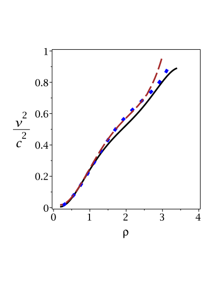
Figure 8: Sound speed ($v^{2}/c^{2}$) versus the density ($\rho\times 10^{15}$ (g/$cm^{3}$)) for $B=0$ (continuous line), $B=5\times 10^{18}G$ (dotted line), and $B=1\times 10^{19}G$ (dashed line).

In order to do more investigations of the EoS introduced in this paper, we analyze both energy and stability conditions. We examine the energy conditions, such as null energy condition (NEC), weak energy condition (WEC), strong energy condition (SEC), and also dominant energy condition (DEC) at the center of neutron stars. The requirements of each energy conditions can be summarize as

$$NEC \rightarrow \ P_{c}+\rho_{c}\geq 0,$$ (32)

$$WEC \rightarrow \ P_{c}+\rho_{c}\geq 0,\ \ \ \&\ \ \rho_{c}\geq 0,$$ (33)

$$SEC \rightarrow \ P_{c}+\rho_{c}\geq 0,\ \ \ \&\ \ 3P_{c}+\rho_{c}\geq 0,$$ (34)

$$DEC \rightarrow \ \rho_{c}>\left|P_{c}\right|,$$ (35)

in which $\rho_{c}$ and $P_{c}$ are, respectively, the density and pressure at the center ($r=0$) of a magnetized neutron star. Using Fig. 7 and the above conditions (32-35), we obtain the results related to the energy conditions in table 5.

Table 5: Energy conditions for a neutron star.

$B(G)$	$\rho_{c}\ (10^{15}g/cm^{3})$	$P_{c}\ (10^{15}g/cm^{3})$	$NEC$	$WEC$	$SEC$	$DEC$
$\begin{array}[]{c}0.0\\ 5\times 10^{18}\\ 1\times 10^{19}\end{array}$	$\begin{array}[]{c}3.896\\ 3.134\\ 2.977\end{array}$	$\begin{array}[]{c}1.910\\ 1.244\\ 1.218\end{array}$	$\begin{array}[]{c}\checkmark\\ \checkmark\\ \checkmark\end{array}$	$\begin{array}[]{c}\checkmark\\ \checkmark\\ \checkmark\end{array}$	$\begin{array}[]{c}\checkmark\\ \checkmark\\ \checkmark\end{array}$	$\begin{array}[]{c}\checkmark\\ \checkmark\\ \checkmark\end{array}$

Our results show that all energy conditions are satisfied (see table 5). So, this EoS of magnetized neutron star matter is suitable to study the properties of magnetized neutron stars. In order to examine the stability of EoS for a physically acceptable model, one expects that the velocity of sound, $v$, be less than the light’s velocity, $c$, Herrera ; Abreu . Considering the relation, $v^{2}=\left(\frac{dP}{d\rho}\right)$, we have presented the sound speed versus density in Fig. 8. It is evident that for all magnetic fields, the EoS of magnetized neutron star matter satisfies the inequality $0\leq v^{2}\leq c^{2}$ (see Fig. 8). Furthermore Le Chatelier’s principle is another stability condition that should be fulfilled. The establishment of this condition indicates that both as a whole and also with respect to the non-equilibrium elementary regions with spontaneous contraction or expansion, the object is stable Ruffini ; Glendenning . It is evident from Fig. 7 that Le Chatelier’s principle is satisfied. Therefore, the EoS of magnetized neutron star matter satisfied both energy and stability conditions.

References

- (1) E. J. Ferrer, V. de la Incera, J. P. Keith, I. Portillo and P. L. Springsteen, Phys. Rev. C 82, 065802 (2010).
- (2) Y. F. Yuan and J. L. Zhang, Astron. Astrophys. 335, 969 (1998).
- (3) T. Tatsumi, Phys. Lett. B 489, 280 (2000).
- (4) R. C. Tolman, Proc. Nat. Acad. Sc. 20, 169 (1934).
- (5) R. C. Tolman, Phys. Rev. 55, 364 (1939).
- (6) J. R. Oppenheimer and G. M. Volkoff, Phys. Rev. 55, 374 (1939).
- (7) R. R. Silbar and S. Reddy, Am. J. Phys. 72, 892 (2004).
- (8) G. Narain, J. Schaffner-Bielich and I. N. Mishustin, Phys. Rev. D 74, 063003 (2006).
- (9) G. H. Bordbar, M. Bigdeli and T. Yazdizade, Int. J. Mod. Phys. A 21, 5991 (2006).
- (10) P. Boonserm, M. Visser and S. Weinfurtner, Phys. Rev. D 76, 044024 (2007).
- (11) X. Li, F. Wang and K. S. Cheng, JCAP 10, 031 (2012).
- (12) A. M. Oliveira, H. E. S. Velten, J. C. Fabris and I. G. Salako, Eur. Phys. J. C 74, 3170 (2014).
- (13) X. T. He, F. J. Fattoyev, B. A. Li and W. G. Newton, Phys. Rev. C 91, 015810 (2015).
- (14) N. Yunes and M. Visser, Int. J. Mod Phys. A 18, 3433 (2003).
- (15) J. S. Heyl and L. Hernquist, Mon. Not. R. Astron. Soc. 324, 292 (2001).
- (16) C. Y. Cardall, M. Prakash and J. M. Lattimer, Astrophys. J. 554, 322 (2001).
- (17) K. Kiuchi, M. Shibata and S. Yoshida, Phys. Rev. D 78, 024029 (2008).
- (18) R. Ciolfi, V. Ferrari and L. Gualtieri, Mon. Not. R. Astron. Soc. 406, 2540 (2010).
- (19) L. L. Lopes and D. P. Menezes, Braz. J. Phys. 42, 428 (2012).
- (20) C. Chirenti and J. Skakala, Phys. Rev. D 88, 104018 (2013).
- (21) M. K. Cheoun, C. Deliduman, C. Güngör, V. Keles, C. Y. Ryu, T. Kajino and G. J. Mathews, JCAP 10, 021 (2013).
- (22) R. Belvedere, J. A. Rueda and R. Ruffini, Astrophys. J. 799, 23 (2015).
- (23) D. Neilsen, S. L. Liebling, M. Anderson, L. Lehner, E. O’Connor and C. Palenzuela, Phys. Rev. D 89, 104029 (2014).
- (24) L. L. Lopes and D. P. Menezes, JCAP 08, 002 (2015).
- (25) F. Kamiab, A. E. Broderick and N. Afshordi, arXiv:1503.03898
- (26) A. E. Broderick, M. Prakash and J. M. Lattimer, Astrophys. J. 537, 351 (2000).
- (27) A. V. Astashenok, S. Capozziello and S. D. Odinstov, Astrophys. Space Sci. 355, 333 (2015).
- (28) S. Perlmutter et al., Astrophys. J. 517, 565 (1999).
- (29) S. Perlmutter, M. S. Turner and M. White, Phys. Rev. Lett. 83, 670 (1999).
- (30) A. G. Riess et al., Astrophys. J. 607, 665 (2004).
- (31) P. Horava, Phys. Rev. Lett. 102, 161301 (2009).
- (32) J. Magueijo and L. Smolin, Class. Quantum Grav. 21, 1725 (2004).
- (33) R. Garattini and E. N. Saridakis, Eur. Phys. J. C 75, 343 (2015).
- (34) G. Amelino-Camelia, Nature. 418, 34 (2002).
- (35) J. J. Peng and S. Q. Wu, Gen. Relativ. Gravit. 40, 2619 (2008).
- (36) A. F. Ali, Phys. Rev. D 89, 104040 (2014).
- (37) S. H. Hendi, M. Faizal, B. Eslam Panah and S. Panahiyan, Eur. Phys. J. C 76, 296 (2016).
- (38) S. H. Hendi, S. Panahiyan, B. Eslam Panah and M. Momennia, Eur. Phys. J. C 76, 150 (2016).
- (39) Y. Ling, X. Li and H. Zhang, Mod. Phys. Lett. A 22, 2749 (2007).
- (40) H. Li, Y. Ling and X. Han, Class. Quantum Grav. 26, 065004 (2009).
- (41) A. F. Ali, M. Faizal and B. Majumder, EPL 109, 20001 (2015).
- (42) P. Galan and G. A. Mena Marugan, Phys. Rev. D 74, 044035 (2006).
- (43) Y. Gim and W. Kim, JCAP 05, 002 (2015).
- (44) A. Awad, A. F. Ali and B. Majumder, JCAP 10, 052 (2013).
- (45) S. H. Hendi, M. Momennia, B. Eslam Panah and M. Faizal, Astrophys. J. 827,153 (2016).
- (46) Y. Ling, JCAP 08, 017 (2007).
- (47) S. H. Hendi, M. Momennia, B. Eslam Panah and S. Panahiyan, Phys. Dark Universe 16, 26 (2017).
- (48) S. Shapiro and S. Teukolsky, Black Holes, White Dwarfs and Neutron Stars. Wiley, New York (1983).
- (49) D. Psaltis, Living Rev. Relativ. 11, 9 (2008).
- (50) K. Y. Eksi, C. Gungor and M. M. Turkoglu, Phys. Rev. D 89, 063003 (2014).
- (51) S. Chandrasekhar, Astrophys. J. 140, 417 (1964).
- (52) J. M. Bardeen, K. S. Thonre and D. W. Meltzer, Astrophys. J. 145, 505 (1966).
- (53) H. Kuntsem, Mon. Not. R. Astron. Soc. 232, 163 (1988).
- (54) M. K. Mak and T. Harko, Eur. Phys. J. C 73, 2585 (2013).
- (55) M. Kalam, S. M. Hossein and S. Molla, arXiv:1510.07015
- (56) H. A. Buchdahl, Phys. Rev. 116, 1027 (1959).
- (57) R. Moradi, C. Stahl, J. Firouzjaee and S. S. Xue, arXiv:1705.04168
- (58) S. Ray, A. L. Espindola, M. Malheiro, J. P. S. Lemos and V. T. Zanchin, Phys. Rev. D 68, 084004 (2003).
- (59) S. H. Hendi, G. H. Bordbar, B. Eslam Panah and S. Panahiyan, JCAP 09, 013 (2016).
- (60) G. Amelino-Camelia, J. R. Ellis, N. Mavromatos, D. V. Nanopoulos and S. Sarkar, Nature. 393, 763 (1998).
- (61) U. Jacob, F. Mercati, G. Amelino-Camelia and T. Piran, Phys. Rev. D 82, 084021 (2010).
- (62) G. Amelino-Camelia, Living Rev. Relativ. 16, 5 (2013).
- (63) J. Magueijo and L. Smolin, Phys. Rev. Lett. 88, 190403 (2002).
- (64) M. L. Rawls et al., Astrophys. J. 730, 25 (2011).
- (65) P. Demorest, T. Pennucci, S. Ransom, M. Roberts and J. Hessels, Nature. 467, 1081 (2010).
- (66) J. Antoniadis et al. Science. 340, 6131 (2013).
- (67) J. S. Clark et al., Astron. Astrophys. 392, 909 (2002).
- (68) P. C. C. Freire et al., Astrophys. J. 675, 670 (2008).
- (69) Jr. C. E. Rhoades and R. Ruffini, Phys. Rev. Lett. 32, 324 (1974).
- (70) P. Haensel, J. P. Lasota and J. L. Zdunik, Astron. Astrophys. 344, 151 (1999).
- (71) C. G. Boehmer and T. Harko, Class. Quantum Grav. 23, 6479 (2006).
- (72) B. C. Paul and R. Deb, Astrophys. Space Sci. 354, 421 (2014).
- (73) S. K. Maurya, Y. K. Gupta, S. Ray and B. Dayanandan, Eur. Phys. J. C 75, 225 (2015).
- (74) D. K. Matondo and S. D. Maharaj, Astrophys. Space Sci. 361, 221 (2016).
- (75) B. S. Ratanpal, V. O. Thomas and D. M. Pandya, Astrophys. Space Sci. 361, 65 (2016).
- (76) N. Andersson and G. L. Comer, Class. Quantum Grav. 18, 969 (2001).
- (77) Z. B. Etienne, Y. T. Liu and S. L. Shapiro, Phys. Rev. D 74, 044030 (2006).
- (78) P. Pani and E. Berti, Phys. Rev. D 90, 024025 (2014).
- (79) R. F. P. Mendes, G. E. A. Matsas and D. A. T. Vanzella, Phys. Rev. D 90, 044053 (2014).
- (80) K. V. Staykov, D. D. Doneva, S. S. Yazadjiev and K. D. Kokkotas, JCAP 10, 006 (2014).
- (81) A. Cisterna, T. Delsate, L. Ducobu and M. Rinaldi, Phys. Rev. D 93, 084046 (2016).
- (82) J. G. Coelho, D. L. Cáceres, R. C. R. de Lima, M. Malheiro, J. A. Rueda and R. Ruffini, Astron. Astrophys. 599, A87 (2017).
- (83) D. Lai and S. L. Shapiro, Astrophys. J. 442, 259 (1995).
- (84) S. Yoshida, S. Karino, S. Yoshida and Y. Eriguchi, Mon. Not. R. Astron. Soc. 316, L1 (2000).
- (85) D. D. Doneva, S. S. Yazadjiev, N. Stergioulas and K. D. Kokkotas, Phys. Rev. D 88, 084060 (2013).
- (86) B. Kleihaus, J. Kunz, S. Mojica and M. Zagermann, Phys. Rev. D 93, 064077 (2016).
- (87) F. Cipolletta, C. Cherubini, S. Filippi, J. A. Rueda and R. Ruffini, Phys. Rev. D 96, 024046 (2017).
- (88) G. H. Bordbar, Z. Rezaei and A. Montakhab, Phys. Rev. C 83, 044310 (2011).
- (89) Z. Rezaei and G. H. Bordbar, Eur. Phys. J. A 52, 132 (2016).
- (90) L. Herrera, Phys. Lett. A 165, 206 (1992).
- (91) H. Abreu, H. Hernandez and L. A. Nunes, Class. Quantum Grav. 24, 4631 (2007).
- (92) N. K. Glendenning, Phys. Rev. Lett. 85, 1150 (2000).