Detector sampling of optical/IR spectra: how many pixels per FWHM?

Abstract

Most optical and IR spectra are now acquired using detectors with finite-width pixels in a square array. Each pixel records the received intensity integrated over its own area, and pixels are separated by the array pitch. This paper examines the effects of such pixellation, using computed simulations to illustrate the effects which most concern the astronomer end-user. It is shown that coarse sampling increases the random noise errors in wavelength by typically $10-20$ % at 2 pixels/FWHM, but with wide variation depending on the functional form of the instrumental Line Spread Function (LSF; i.e. the instrumental response to a monochromatic input) and on the pixel phase. If line widths are determined they are even more strongly affected at low sampling frequencies. However, the noise in fitted peak amplitudes is minimally affected by pixellation, with increases less than about 5%. Pixellation has a substantial but complex effect on the ability to see a relative minimum between two closely-spaced peaks (or relative maximum between two absorption lines). The consistent scale of resolving power presented by Robertson (2013) to overcome the inadequacy of the Full Width at Half Maximum (FWHM) as a resolution measure is here extended to cover pixellated spectra. The systematic bias errors in wavelength introduced by pixellation, independent of signal/noise ratio, are examined. While they may be negligible for smooth well-sampled symmetric LSFs, they are very sensitive to asymmetry and high spatial frequency substructure. The Modulation Transfer Function for sampled data is shown to give a useful indication of the extent of improperly sampled signal in an LSF. The common maxim that 2 pixels/FWHM is the Nyquist limit is incorrect and most LSFs will exhibit some aliasing at this sample frequency. While 2 pixels/FWHM is nevertheless often an acceptable minimum for moderate signal/noise work, it is preferable to carry out simulations for any actual or proposed LSF to find the effects of various sampling frequencies. Where spectrograph end-users have a choice of sampling frequencies, through on-chip binning and/or spectrograph configurations, it is desirable that the instrument user manual should include an examination of the effects of the various choices.

1 INTRODUCTION

Detectors with pixels on a square array are in widespread use in current optical and IR grating spectrographs. A key issue confronting the designer or user of such instruments is the size of the individual detector pixels with respect to the width of the instrumental profile - in other words how many pixels should be used to sample the width of an unresolved spectral line. If too few pixels are used, narrow or unresolved spectral features will be undersampled, resulting in errors of position (i.e. wavelength) and possibly also flux which vary depending on the phase of the spectral line with respect to the pixel centres. The ability to distinguish closely spaced lines will be compromised, as will detection of slight broadening of a spectral feature. Random errors in wavelength and width are also increased with coarse sampling. On the other hand, if an unnecessarily large number of pixels are used to span the instrumental width, then the spectrograph’s total wavelength range will be reduced for a given detector size, and the effects of readout noise, dark noise and cosmic ray hits will be exacerbated.

The approach that has most often been taken in the literature is to say that 2 pixels per Full Width at Half Maximum (FWHM) represents Nyquist sampling, which is satisfactory but a bare minimum, and that for more accurate work (such as accurate radial velocities or velocity dispersions) a larger number of pixels such as 3 to 4 per FWHM should be used. However, 2 pixels per FWHM is not the Nyquist limit and the minimum acceptable sampling frequency depends on the required accuracy and on the form of the instrumental profile, here referred to as the Line Spread Function (LSF).

The CCD and IR array detectors perform two operations on the LSF as it falls on the detector, in the process of sampling (e.g. Bernstein 2002): firstly the light which falls within the area of a single pixel is integrated over the finite area of the pixel, and secondly a single intensity value is recorded and nominally ascribed to the location at the centre of the pixel. In this work the pixels will be regarded as having uniform sensitivity across their width (except in Section 10.1).

Using Fourier Transform methods it is quite straightforward to take any proposed LSF, convolve it with a rectangle representing the smoothing effect of integrating the signal over the pixel width, and then find the extent to which the Fourier components lie beyond the true Nyquist frequency (i.e. 2 samples per cycle of a sinusoid) for any given sampling frequency. However, this does not answer the questions which concern the instrument scientist or astronomer, namely what level of errors will be introduced into the measurement of wavelengths, line strengths and widths, and how will the ability to separate two closely-spaced spectral lines be affected? This paper aims to make a start towards answering these more practical questions. The approach will be to illustrate the effects of sampling, rather than to give another mathematical analysis.

Spectra will be assumed to be 1-dimensional, i.e. representing an array giving intensity as a function of wavelength. The integration or extraction over the spatial dimension to produce such 1-dimensional spectra is not the issue here, and the emphasis is on adequacy or otherwise of sampling as a function of wavelength. Data samples will be assumed to be digitised with sufficient precision that quantisation noise can be neglected.

A comprehensive introduction to the basics of the sampling process is given by Vollmerhausen et al (2010); see also Anderson & King (2000). Bickerton & Lupton (2013) presented Fourier methods to give accurate photometry of sampled images.

2 EFFECTS OF SAMPLING

Sampling by pixels with uniform sensitivity and no interpixel gaps (as assumed above) has a number of effects:

1) The integration of the received intensity signal over the width of a pixel has the effect of smoothing the incident intensity profile, through convolution with a rectangular profile having the width of one pixel. This broadens the effective LSF and hence reduces the spectral resolving power of the instrument, in the sense that it cannot resolve two closely spaced spectral lines as well as before sampling.

2) The noise errors of the key parameters of spectral lines - namely position (wavelength) and width will be increased, and the flux errors will be increased unless an integrated flux is used.

3) If sampling is inadequate (i.e. too coarse) then systematic bias errors may be introduced in the fitted line parameters.

4) Coarse sampling may reduce the ability to distinguish closely spaced spectral features.

While simple in principle, the quantification of the above errors is complicated by the fact that the errors do not depend solely on the sampling rate and the LSF functional form - they also depend on the type of analysis performed on the spectral data. This analysis can take many forms - such as fitting a Gaussian or series of Gaussians to spectral features (although the LSF will in general not be an exact Gaussian), or fitting another functional form, or calculation of a centroid wavelength, or perhaps interpolation (referred to as ‘reconstruction’ in the literature on 2D imaging). An important special case is the fitting of the exactly correct LSF (including allowance for the convolution effect of the finite pixel width) to unresolved spectral features. In this case unbiased wavelengths can be obtained even with significant undersampling, because the process is analogous to deconvolution.

The analysis and discussion below attempts to find within this complex multi-dimensional problem some results which are useful to designers and users of sampled spectrographs.

3 WAVELENGTH ACCURACY

It is expected that coarse pixellation will increase the random wavelength uncertainty in locating an unresolved spectral feature. The conceptually simplest view is that the effective LSF is the intrinsic (instrumental) LSF convolved with the pixel rectangle - this necessarily broadens the LSF and hence diminishes the wavelength accuracy. However, the simple view does not take into account the dependence on pixel phase, which is important at low sampling frequency, so we proceed as follows. (The results here are given assuming positive-going peaks, but would be equally applicable to weak absorption features which leave the per-pixel noise approximately constant.)

Defining $\sigma$ as the rms noise in each pixel (wavelength channel) and assuming the noise is constant per unit wavelength interval (at least in the vicinity of a given spectral feature) and that the noise in separate pixels is uncorrelated, the formula for wavelength uncertainty $\sigma_{\lambda}$ given by Clarke et al. (1969) can be used:

$$\sigma_{\lambda}^{2}=\frac{\sigma^{2}}{{\rm pk}^{2}\Big{(}\sum{(B^{\prime})^{2}}-\Big{(}\sum{BB^{\prime}}\Big{)}^{2}/\sum{B^{2}}\Big{)}}$$ (1)

where ‘pk’ is the peak amplitude of the response whose $\sigma_{\lambda}$ is to be found. $B^{\prime}$ is the derivative with respect to wavelength of the LSF $B$, which is assumed normalised to a peak of unity (before pixel convolution). Some care is needed in the evaluation of $B^{\prime}$ when pixels are wide and the slope may change greatly across one pixel. Inspection of the Clarke et al. derivation shows that $B^{\prime}$ for a given pixel refers to $dB/d\lambda$ where $B$ is interpreted as the continuous (i.e. unsampled) LSF but integrated across the pixel and then point sampled at the relevant pixel centre. Thus eqn (1) may be conveniently evaluated for any LSF that is known as a continuous function, by first convolving with the pixel rectangle and then sampling $B$ and $B^{\prime}$ at the appropriate locations. The validity of the formula for coarsely pixellated data treated in this way has been verified by Monte Carlo tests.

In the case of a well-sampled symmetric LSF observing an unresolved spectral feature, this equation simplifies to :

$$\sigma_{\lambda}^{2}=\sigma^{2}/\Big{(}{\rm pk}^{2}\sum{(B^{\prime})^{2}}\Big{)}.$$ (2)

However, the general form (1) will be used here in order to handle coarse sampling correctly. The results for a number of LSF forms will now be examined.

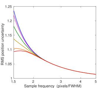
Figure 1: Wavelength uncertainty vs sampling frequency for a range of pixel phase values. The LSF form is Gaussian. The uppermost (blue) curve corresponds to pixel phase = 0 (peak centred on a pixel) while the lowest (red) curve, which has a maximum at sample frequency $\sim 1.64$, is for pixel phase = $\pm 0.5$, i.e. a peak lying on the boundary between two pixels. Other curves have pixel phases at intervals of 0.1. The noise in each pixel is uncorrelated and is appropriately scaled for the actual pixel widths, such that the noise for unit dispersion axis interval remains constant. The vertical scale of RMS position uncertainties has been normalised to unity at very large sample frequency.

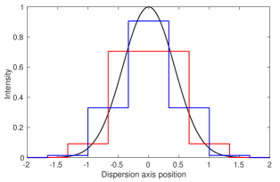
Figure 2: Gaussian LSF (black) with superposed sampled versions of the same LSF (blue: pixel phase 0, red: pixel phase 0.5). The sampling frequency is 1.5 pixels/FWHM.

Figure 1 shows the variation of random wavelength error with sampling frequency for the case of a Gaussian LSF. All curves show a rise in position errors as the sampling frequency decreases. This is expected due to the lessened sensitivity of wide pixels to the steep sides of the LSF. Below about 2 pixels per FWHM there is increasing dependence of the result on the pixel phase. The greatest errors occur for the LSF peak centred in the middle of a pixel, while for the LSF centred on the boundary between two pixels, errors are minimised and there is actually a turn-over, with coarser pixellation resulting in lower position errors. This can be understood as the pair of pixels starting to act as one axis of a quad-cell position locator (i.e using the flux ratio between the two adjacent pixels to determine the peak location). The red line in Figure 2 shows the LSF straddling the boundary of two pixels for a sampling frequency of 1.5 pixels/FWHM, illustrating the rapid shift of flux between the two major pixels, as the peak shifts slightly with respect to the pixels.

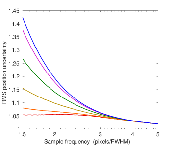
Figure 3: Wavelength uncertainty vs sampling frequency for a Lorentzian LSF, otherwise as for Figure 1.

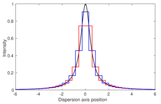
Figure 4: Lorentzian LSF (black) with superposed sampled versions of the same LSF (blue: pixel phase 0, red: pixel phase 0.5). The sampling frequency is 1.75 pixels/FWHM.

Figure 3 shows the similar set of curves, in this case for a Lorentzian LSF. The sharpness of the Lorentzian’s core with respect to its wings results in a pronounced dependence of the wavelength error on pixel phase. Thus the red line in Figure 4, at pixel phase 0.5, shows the case where the ‘quad-cell’ effect holds the wavelength error nearly constant with decreasing sample frequency. On the other hand, the blue line, at pixel phase 0, corresponds to sharply increased $\sigma_{\lambda}$.

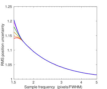
Figure 5: Wavelength uncertainty vs sampling frequency for a sinc² LSF. Since the sinc² function has minor lobes with amplitudes decaying slowly away from the central peak, it is not possible to include all the function’s non-zero values as was effectively done for other LSFs. In this case the summations were continued to dispersion axis positions of $\pm 225.76\times{\rm FWHM}$, in order to obtain a close approximation to the band-limited nature of sinc². The pixel phase curves are coloured as in Figure 1.

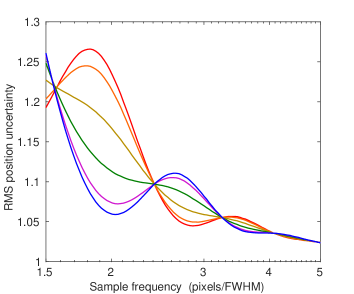
Figure 6: Wavelength uncertainty vs sampling frequency for a range of pixel phase values. The LSF form is the convolved projected circle. At a sample frequency of 2 pixels/FWHM, the lowest (blue) curve corresponds to pixel phase = 0 (peak centred on a pixel) while the highest (red) curve is for pixel phase = $\pm 0.5$. Other curves again have pixel phases at intervals of 0.1.

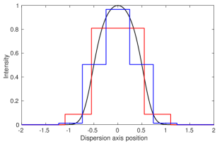
Figure 7: Convolved projected circle LSF (black) with superposed sampled versions of the same LSF (blue: pixel phase 0 at 2.03 pixels/FWHM (i.e. at the local minimum of the position uncertainty curve), red: pixel phase 0.5 at sampling frequency 1.82 pixels/FWHM (i.e. at the local maximum)).

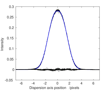
Figure 8: Arc line profile from AAOmega, using a subarea of 1000 (spatial) x 500 (wavelength) pixels near the centre of the data frame. 266 unblended and unsaturated fibre images were selected for processing. The horizontal axis is in units of pixels, and the vertical axis is intensity in arbitrary units. The blue curve is a 3-parameter empirical fit, $I=0.2800\exp(-0.1854|p|^{2.4174})$ where $p$ is the horizontal axis independent parameter in pixels. The residuals with respect to this fit are also shown - indicating that the fit is good but not perfect. The fitted curve has FWHM = 3.450 pixels.

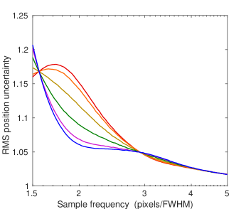
Figure 9: Wavelength uncertainty vs sampling frequency for a range of pixel phase values. The LSF is from the AAOmega spectrograph. At a sample frequency of 2 pixels/FWHM, the lowest (blue) curve corresponds to pixel phase = 0 (peak centred on a pixel) while the highest (red) curve is for pixel phase = $\pm 0.5$. Other curves again have pixel phases at intervals of 0.1. (The actual sample frequency for the intrinsic LSF of AAOmega is 3.41 pixels/FWHM.)

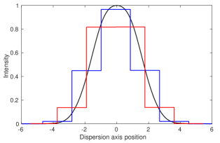
Figure 10: AAOmega spectrograph LSF (black) with superposed sampled versions of the same LSF (blue: pixel phase 0, red: pixel phase 0.5). The sampling frequency is 2.0 pixels/FWHM (not equal to the actual as-built pixel scale). The unsampled LSF has a FWHM of 3.41.

Figure 5 shows the $\sigma_{\lambda}$ vs sampling frequency curves for a sinc² LSF. This LSF form arises in the case of a diffraction-limited slit, and has the important property that its Fourier Transform is band-limited, i.e. if it is sampled at or above the Nyquist rate, there will be no aliasing. This topic will be expanded in Section 9 but the important point to note from Figure 5 is that the divergence of the curves for different pixel phases begins below the sampling frequency of 1.77 pixels/FWHM, which corresponds closely to Nyquist sampling. In other words, where there is no aliasing, there is also no dependence of $\sigma_{\lambda}$ on pixel phase.

The next LSF to be considered is intended to represent the result of projecting the image of a multi-mode fibre on to the wavelength axis. The ideal result is a half ellipse (e.g. Bracewell 1995), but the extremely steep sides of the ellipse will inevitably be smoothed to some extent by optical aberrations in the spectrograph, so what is used here is the projected circle convolved with the Gaussian that produces the minimum final FWHM (Robertson 2013, hereafter referred to as Paper 1). This provides an example representative of projected multi-mode fibres subject to some spectrograph aberrations. Figure 6 shows the variation of random wavelength errors with sampling frequency and pixel phase. The oscillatory behaviour, with pixel phase 0 being best at some sampling frequencies, and phase 0.5 best at others, is radically different from the Gaussian, Lorentzian and sinc² cases. The reason is the steep-sided and flat-topped nature of the LSF. As equations 1 and 2 show, the accuracy of wavelength determination depends on the regions of greatest slope. Thus $\sigma_{\lambda}$ will be minimised at the pixel phases and sampling frequencies that are able to derive good position discrimination from both sides of the LSF. The red line in Figure 7 shows the sampled LSF at pixel phase 0.5 and sample frequency 1.82 pixels/FWHM, which is a local maximum in $\sigma_{\lambda}$. In this configuration there is minimal sensitivity of the relative pixel intensities to small changes in wavelength, due to the flat-topped nature of the LSF. On the other hand the blue line in Figure 7 shows pixel phase 0 at 2.03 pixels/FWHM, giving a local minimum of $\sigma_{\lambda}$. Here, a small shift of the LSF with respect to the pixels produces a maximal change in values for the pixels on either side of the centre. The flattened top of the LSF in effect decouples the contributions of the two sides, resulting in particular combinations of pixel phase and sample frequency that are optimum.

The final LSF is that of an actual spectrograph, the AAOmega instrument operating at the Anglo-Australian Telescope (Saunders et al. 2004). This instrument uses multi-mode fibres and thus can be expected to give results similar to those of the convolved projected circle. It is nevertheless interesting to see whether curves such as Figure 6 are borne out in practice. An arc frame of CCD data from AAOmega was used, and 266 fibre images were selected from the central part of the CCD where the LSF is sufficiently constant. Each fibre image was projected to the wavelength axis, then images were aligned to their centroid and scaled to flux equality and plotted together, as shown by the black points in Figure 8. Because there is some tilt of the lines along the AAOmega spatial axis, and also a number of lines of different wavelength were used, the result is good coverage of all pixel phases (i.e. position of centroid with respect to the pixel boundaries). There are 266 fibre profiles with an average of 14.3 points per profile, giving 3800 points, hence virtually continuous coverage of the LSF.

What this shows (as the set of black plotted points) is the true LSF received by the detector, after convolution with the pixel response. Anderson & King (2000) refer to this as the effective PSF (ePSF).

As expected, this LSF cannot be satisfactorily fitted with a Gaussian, because the peak is too broad and the wings too low relative to the best-fit Gaussian. The blue curve in Figure 8 shows an empirical fit that is adequate for the present purposes. Using that fit the LSF profile was successfully deconvolved to remove the effect of pixel convolution, assuming the pixel response is a perfect rectangle of width 1 pixel. Because the profile is well sampled, pixel deconvolution makes only a minimal difference.

The deconvolved LSF represents the LSF as it fell on the detector, so it can be used as input to calculation of $\sigma_{\lambda}$ vs sampling frequency as before. Figure 9 shows the results. Indeed the oscillations do occur, although at the actual AAOmega sampling frequency of 3.41 pixels/FWHM, there is minimal dependence on pixel phase. But if 2-pixel sampling had been adopted, it would have been quite significant.

Figure 10 shows the deconvolved AAOmega LSF and its pixellation at phases 0 and 0.5.

The results given in this section show that sampling at 2 pixels/FWHM causes a loss of typically $10-20$% in wavelength accuracy relative to the limit of continuous sampling. There is, however, a considerable variation among the different LSF forms, and increasing dependence on pixel phase for coarse sampling.

4 WIDTH ACCURACY

Pixellation has an even greater effect on the accuracy of width measurements for barely resolved spectral features, such as in the measurement of galaxy velocity dispersions. It is intuitively obvious that coarse pixellation will impede the determination of an accurate width measurement. In this section examples of two LSFs are given to illustrate this point.

When three parameters (location, peak height and width) are to be fitted to a profile, it is not possible to give an explicit equation for the width uncertainties that is analogous to equation (1). Instead the procedure adopted was to use the non-linear least squares fitting facility nlinfit in matlab. The input data set was the (unbroadened) LSF sampled at the appropriate sampling frequency and pixel phase, and the fitting function was the same LSF. With starting values for the location, peak height and FWHM deliberately differing from the correct values by $5-10$%, nlinfit then determined the best fit parameter values (using the correct integration across pixels for the fitting function). Instead of injecting noise and then performing numerous Monte Carlo simulations to assess the scatter of fitted parameter values, use was made of the Jacobian matrix $J$ of the non-linear regression model, which can be returned by nlinfit. Calculation of $\sigma^{2}(J^{T}*J)^{-1}$ gives the covariance matrix of the three parameters, when the noise is assumed to be independent and have the same RMS value $\sigma$ in each pixel.

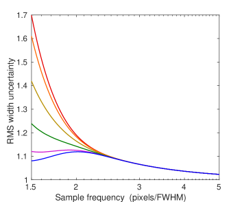
Figure 11: Width uncertainty vs sampling frequency for a range of pixel phase values. The LSF is Gaussian. The lowest (blue) curve corresponds to pixel phase = 0 (peak centred on a pixel) while the highest (red) curve is for pixel phase = $\pm 0.5$. Other curves have pixel phases at intervals of 0.1. The noise in each pixel is uncorrelated and is appropriately scaled for the actual pixel widths, such that the noise for unit dispersion axis interval remains constant. The vertical scale of RMS width uncertainties has been normalised to unity at very large sample frequency.

Figure 11 shows the results for a Gaussian LSF. Since the input function and the fitting function were both unbroadened, the results represent the noise in width for small width extensions. The plots have been normalised to unity at large sample frequencies, i.e. the numerical values again show the factor by which sampling increases the noise. This Figure shows that pixel phase dependence develops below about 2.4 pixels/FWHM, and worsens rapidly below 2 pixels/FWHM. In contrast to the case for wavelength uncertainties, the lowest errors for width are obtained at pixel phase 0 (peak centred on a pixel) and the worst at pixel phase $\pm 0.5$ (peak at the boundary of two pixels). This can be understood since in the latter case the width determination will rely on the values in the two pixels either side of the central two, and there is little signal in them at low sample frequencies (e.g. the red histogram pixels at $\pm 1$ in Figure 2). Saunders (2014) also noted that the best pixel phase for position (wavelength) determination is the worst for widths.

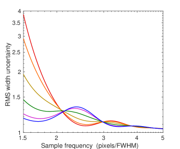
Figure 12: Width uncertainty vs sampling frequency for the convolved projected circle LSF. The colour coding for pixel phases is as before.

Figure 12 shows the corresponding plot for the convolved projected circle LSF. In this case the steep sides and low wings of the LSF exacerbate the problem of finding widths at pixel phase 0.5 and low sample frequencies, and as a result at 1.5 pixels/FWHM it reaches an RMS width error almost $4\times$ worse than the fine-sampled limit. Any sampling frequency below 2 pixels/FWHM experiences severe noise enhancement at pixel phases close to 0.5. Even at 2.5 pixels/FWHM there is significant pixel phase $-$ dependent enhancement of the width uncertainties.

5 PEAK ACCURACY

This section considers the effect of pixellation on the random noise errors affecting the peak amplitude of an unresolved spectral feature. Clarke et al. (1969) give an equation analogous to equation (1) for the uncertainty of the peak amplitude, when making a 2-parameter least squares fit to an unresolved feature:

$$\sigma_{\rm pk}^{2}=\frac{\sigma^{2}}{\sum{B^{2}}-\Big{(}\sum{BB^{\prime}}\Big{)}^{2}/\sum{(B^{\prime})^{2}}}.$$ (3)

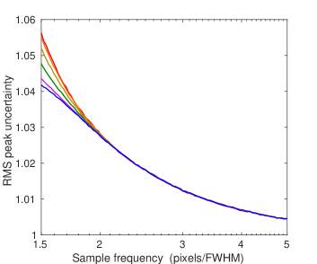
Figure 13: Peak uncertainty vs sampling frequency for the Gaussian LSF. As before, the noise is constant per unit wavelength interval, and is independent from one pixel to the next. The uncertainties are normalised to unity at large sampling frequency, in order to show the effects of pixellation. The colour coding for pixel phases is as before.

Figure 13 shows the result for a Gaussian LSF. As with wavelength (position) and width uncertainties, pixel phase dependence develops below about 2 pixels/FWHM. However the average effects are small, with less than 3% increase in noise at 2 pixels/FWHM due to pixellation. The largest errors occur for pixel phase 0.5, where the signal is spread out over a larger effective number of pixels than for pixel phase 0.

Since $\sigma_{\rm pk}$ and the pixel noise $\sigma$ have the same dimensions, they can be validly compared. Defining $n_{\rm eff}$ as the effective number of pixels in the ‘resolution element’,

$$\sigma_{\rm pk}^{2}=\frac{\sigma^{2}}{n_{\rm eff}},$$ (4)

and equation 3 could be used to find $n_{\rm eff}$ .

Figure 14 shows the corresponding change in $\sigma_{\rm pk}$ for the convolved projected circle. Again the average increase in errors due to pixellation is small, less than about 4% at 2 pixels/FWHM.

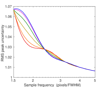
Figure 14: Peak uncertainty vs sampling frequency for the convolved projected circle LSF. The colour coding for pixel phases is as before.

6 CONSISTENT SCALE OF SPECTRAL RESOLVING POWER

Sampling by finite-width pixels causes a reduction in spectral resolving power, since the effective LSF is the unsampled LSF convolved with a rectangle equal to the pixel width. While it is possible to calculate a resolving power loss by simply comparing the widths of the original LSF as incident on the detector and the width after pixel convolution, this gives only an average over pixel phases, and does not show the important differences which arise as a function of pixel phase at low sampling frequency. Moreover, as will be shown below, it does not give an accurate picture of the effects of pixellation on the various LSF forms.

The obvious difficulty in calculating a pixel-phase dependent resolving power lies in how resolving power should be defined in the case of coarse sampling. The approach taken here follows that of Paper 1, where it was argued that the modern conventional definition of spectral resolving power as $R=\lambda/\delta\lambda$ with $\delta\lambda$ taken as the FWHM is unsatisfactory because FWHM is a poor measure of the truly important aspects of resolution, namely the ability to distinguish closely-spaced spectral lines, or to measure accurate wavelengths of unresolved lines. Taking the latter property as the basis, a consistent measure of resolution $\delta\lambda_{\sigma\lambda}=\beta$ FWHM was developed. The formula for calculation of $\beta$ was given for the case where the LSF is continuous or finely sampled. We now consider the important case of pixellated data. (The other consistent resolving power scale of Paper 1, based on the ‘$\alpha$’ scaling factors, will not be considered here because the ‘$\beta$’ scale is easier to use in practice. However, Section 8 does consider one effect of sampling on resolution of closely-spaced features.)

This approach will take into account both the broadening effect of the sampling (effectively convolution of the LSF with the pixel rectangle) and the increase of wavelength error due to pixellation, as seen in Figures 1, 3, 6, and 9. In this context ‘wavelength uncertainty’ refers to random noise errors - the bias errors which also depend on pixel phase but which are not diminished by high signal/noise data are considered later.

The analysis requires knowledge of the ‘intrinsic LSF’, which is used to mean the continuous LSF that has fallen on the detector, before sampling. This is known in the case of model LSFs such as the Gaussian, Lorentzian and the convolved projected circle, and could also apply to smooth model LSFs derived from optical design software models or an empirical LSF processed as for the AAOmega LSF above (with deconvolution to remove the effects of pixel sampling, at least approximately). With the intrinsic LSF known, the effects of any proposed sampling frequency can be evaluated.

Following Paper 1 the ‘$\beta$’ scale of consistently-defined resolving power is based on equating the wavelength errors for the LSF in question and that of a sinc² LSF, i.e.

$$\sigma_{{\lambda}\ ({\rm sinc}^{2},{\rm cont})}=\sigma_{{\lambda}\ ({\rm LSF,pix,phase})}$$ (5)

where the left-hand side represents the $\sigma_{\lambda}$ of a sinc² LSF that is continuous or very finely sampled, while the right hand side is the $\sigma_{\lambda}$ of the LSF under study, which is pixellated and observed at some particular pixel phase. Thus given a certain LSF form, sampling frequency and pixel phase, equation 5 can be used to give the FWHM of the sinc² profile required to satisfy the equality.

The analysis will closely follow that of Paper 1. Since a variety of pixel widths are now considered it is necessary to write the spectral noise as

$$\sigma_{1}=\sigma\sqrt{\Delta\lambda}.$$ (6)

Here $\sigma_{1}$ is the noise for unit wavelength (dispersion axis) interval and is constant both within a spectrum and between the two LSFs considered, while $\sigma$ is then the noise in a pixel (wavelength channel) of width $\Delta\lambda$, and is assumed to be uncorrelated between pixels.

In order to use the Clarke et al. formulas (equations 1 or 2) it is convenient to define $S$ by

$$1/S=\Delta\lambda\Big{(}\sum{(B^{\prime})^{2}}-\Big{(}\sum{BB^{\prime}}\Big{)}^{2}/\sum{B^{2}}\Big{)}$$ (7)

or, if the simple formula is adequate,

$$1/S=\Delta\lambda\Big{(}\sum{(B^{\prime})^{2}}\Big{)}.$$ (8)

$S$ will play the role for pixellated data that the ‘noise width’,

$$Z=\frac{1}{\int_{-\infty}^{+\infty}(B^{\prime})^{2}d\lambda}.$$ (9)

plays for continuous symmetric LSFs. The crucial difference is that $S$ depends on the sample frequency and pixel phase as well as on the LSF form. Following the same procedure as in Paper 1, i.e. equating the RMS wavelength errors for the pixellated LSF and a continuous sinc² LSF under the condition of equal fluxes (peak $\times$ equivalent width) the result is

$$\beta=1.3809\ S^{\frac{1}{3}}_{\rm LSF}{\rm EW}^{\frac{2}{3}}_{\rm LSF}/{\rm FWHM}_{\rm LSF}$$ (10)

where EW stands for the equivalent width (area/peak height). Hence the resolution element which should be used in place of FWHM_LSF is

$$\delta\lambda_{\sigma\lambda}=\beta\ {\rm FWHM}_{\rm LSF}=1.3809\ S^{\frac{1}{3}}_{\rm LSF}{\rm EW}^{\frac{2}{3}}_{\rm LSF}.$$ (11)

The value of $\beta$ reflects the effects of pixellation, LSF form and conversion to the Rayleigh criterion of a sinc² profile to define what ‘just resolved’ means. To calculate the final resolving power on the consistently-defined scale, use

$$R_{\sigma\lambda}=\frac{1}{\beta}\frac{\lambda}{{\rm FWHM}_{\rm LSF}}.$$ (12)

Figure 15 shows the results for the four LSFs discussed in section 3. Rather than assume some arbitrary resolving power for comparison, they are presented as relative resolving power, which is just $1/\beta$ as calculated from equation 10. The factors which affect this plot are: 1) For a given FWHM, the basic LSF form affects the resolving power when measured on the consistent scale which is based on equality of $\sigma_{\lambda}$. This is the reason the Lorentzian’s values are low, while the convolved projected circle is high; 2) Sampling by finite width pixels reduces the resolving power by increasing the wavelength uncertainties as the sample frequency is reduced; 3) Pixel phase becomes increasingly important at low sample frequencies; 4) The absolute values on the vertical scale are relative to the value 0.886 (=1/1.129) which applies to a sinc² LSF with fine sampling and using the Rayleigh criterion to define ‘just resolved’.

The black curves show the result of calculating the resolving power reduction due to sampling by simply convolving the LSF with the pixel rectangle and comparing the FWHM with that of the intrinsic LSF. For convenience, the values have been scaled to agree with the corresponding consistently-defined relative resolving power at the limit of fine sampling. Only for the Gaussian LSF does this simplistic calculation show approximately the correct dependence on sample frequency. For the others it is a poor approximation, especially for the convolved projected circle or the AAOmega LSF - which represent forms encountered in any spectrograph fed by multi-mode fibres. Furthermore, the simplistic calculation is unable to take account of the dependence on pixel phase.

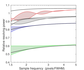
Figure 15: Relative resolving power $R_{\sigma\lambda}/R=1/\beta$, where $R_{\sigma\lambda}$ is the resolving power of the LSF in question, as subject to pixellation and measured on the consistently defined ‘$\beta$’ scale, and $R=\lambda/{\rm FWHM}$ is the conventionally-defined resolving power of the LSF, in the limit of fine sampling. The plot shows the relative values of $R_{\sigma\lambda}/R$ for the four LSFs, when all have the same unsampled FWHM. On this scale, the value 0.886 corresponds to the resolving power of a fine-sampled sinc² LSF (again with the same FWHM), using the Rayleigh criterion to define resolution. The shaded areas indicate the range covered by different pixel phases. From the top the curves are: red - convolved projected circle; grey - AAOmega LSF; blue - Gaussian; green - Lorentzian. The black curves show the effect of pixel convolution on the conventional $R=\lambda/{\rm FWHM}$.

As an example, $R_{\sigma\lambda}$ has been calculated for the AAOmega configuration above, using the deconvolution of the empirical fit to the LSF (shown in Figure 8) and the known centre wavelength (725.21 nm) and dispersion (0.1568 nm/pixel). The above process gives $R_{\sigma\lambda}=1282.8-1286.9$, with the range of values being due to different pixel phases. The range is narrow because the profile is well sampled. For comparison, the conventional $R=\lambda/{\rm FWHM_{\rm LSF}}=1358.7$. In this case the difference between the conventional $R$ and $R_{\sigma\lambda}$ is small (i.e $\beta$ is close to 1), due to two competing effects: the LSF has steeper sides than a sinc² profile, which will raise $R_{\sigma\lambda}$, but then the result is scaled down to give resolving power equivalent to that from the Rayleigh criterion. There is little loss of resolving power due to pixellation because the sampling frequency is 3.41 pixels/FWHM.

7 SYSTEMATIC BIAS ERRORS

As well as the increased random errors described above in Sections 3, 4 and 5, pixellation of a spectrum can also lead to bias errors. In general such errors will depend on the pixel phase of a spectral feature. They are insidious because they differ from the usual noise errors in that they are not reduced by high signal/noise ratio, and thus must eventually dominate (perhaps with other systematic errors) for very high S/N spectra. In that case they would set a quasi-random noise floor, when considering an ensemble of spectral features of various pixel phases. Such errors will occur if the spectral features are fitted using a functional form which does not exactly match the LSF, such as the common practice of fitting (say) a Gaussian to features which are not exactly Gaussian. There are also small bias errors in using the model-independent centroid as a location parameter.

Bias errors in the flux of a spectral line can in principle be easily avoided simply by summing the contributions of the wavelength channels (pixels) which include the line, but this is a noisy process, subject to truncation error in the line wings. Flux bias will be introduced if an incorrect functional form is fitted.

7.1 Exact LSF fitted to spectral features

It is not possible to give a general formula which includes all possible LSFs and fitting functional forms. In general the only approach is to carry out simulations, and a number of these will be presented below. The first case to consider is when the exactly correct functional form is fitted, i.e. the intrinsic LSF is known exactly, and it is integrated over samples for every spectral feature, taking due account of the pixel phase. No plots will be shown for this case because it results in bias-free fitting, even when there is a degree of undersampling (i.e. the LSF contains Fourier components beyond the Nyquist limit).

7.2 Gaussian fits

A common practice in spectral analysis is to fit a Gaussian profile to spectral lines, on the basis that although the LSF is not exactly Gaussian, it is likely to be fairly close. This section examines the resulting biases.

The first case is that of a Gaussian intrinsic LSF, but the fitting function is a plain point-sampled Gaussian, i.e. not integrated across samples. Thus there are misfit errors which are worse for lower sampling frequency. Note that it is necessary to make a 3-parameter fit, allowing a variable width as well as position and peak height, because the fitted form is not the correct one. Figure 16 shows the results for each of the three parameters. The position bias increases rapidly below 2 pixels/FWHM, reaching pixel-phase dependent extremes of $\pm 0.0010$ (0.1% of the FWHM) at 1.5 pixels/FWHM. Such errors would be unimportant in low to moderate signal/noise data, and the crude fit of an inappropriate LSF would not be used in high precision work. The bias errors in peak height and width are substantial at low sampling frequencies, with the effect of functional form mismatch overshadowing the effect of pixel phase. With the peak underestimated and the width overestimated by a similar factor, the flux error is much reduced and reaches only 0.13% at 1.5 pixels/FWHM.

The data of Figure 16a are presented as a function of pixel phase in Figure 17. As expected, the position error is zero when the pixels are symmetric with respect to the peak, at phases 0 and $\pm 0.5$, and varies approximately sinusoidally at other pixel phases. The error decreases rapidly with increasing sample frequency, and is negligible above 2 pixels/FWHM.

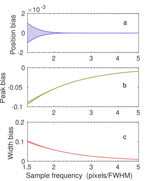
Figure 16: Bias errors of position, peak height and width for a plain Gaussian fitted to a sampled Gaussian LSF. For position and width the errors are relative to the FWHM of 1.0, and the peak bias is relative to the Gaussian LSF peak = 1.0. The filled areas show the range of values covered by different pixel phases. The annotation ‘$\times 10^{-3}$’ on the vertical axis of panel ‘a’ applies only to that panel.

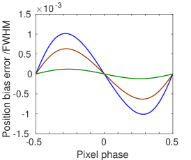
Figure 17: Bias errors of position as a function of pixel phase, for a plain Gaussian fitted to a Gaussian LSF. The highest amplitude curve is for sample frequency of 1.5 pixels/FWHM, the others are at 1.6 and 1.9 pixels/FWHM.

The next LSF considered is the projected circle convolved with the Gaussian which results in the minimum final intrinsic FWHM, as used in Figure 7. The results for biases in position, peak and width for this case are shown in Figure 18. The position bias errors are much larger than for the Gaussian LSF (at sample frequency 1.5 the range is $24\times$ greater), and extend to beyond 2 pixels/FWHM. The peak and width errors also have greatly increased pixel-phase dependence, and unlike Figure 16 the biases do not asymptote to zero at high sample frequency because in this case the Gaussian fit is inherently an incorrect functional form. Quite apart from issues of pixellation, this is an illustration of the danger of using an inappropriate functional form, since these errors would be apparent in even moderate S/N data. For calculation of the flux (area) the peak and width errors again tend to compensate, and the maximum flux error is +3.5% at 2.21 pixels/FWHM.

Figure 19 shows the position bias errors vs pixel phase. Again an approximately sinusoidal form is seen, but with much larger amplitude, which could affect moderate S/N spectra. Figure 20 shows one example of the misfit which occurs when attempting to fit this LSF with a plain Gaussian.

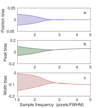
Figure 18: Bias errors of position, peak height and width for a plain Gaussian fitted to an LSF derived from convolution of a projected circle with a Gaussian that gives the minimum final intrinsic FWHM. For position and width the errors are relative to the FWHM of 1.0, and the peak bias is relative to the intrinsic LSF peak = 1.0. The filled areas show the range of values covered by different pixel phases.

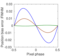
Figure 19: Bias errors of position as a function of pixel phase, for a plain Gaussian fitted to the convolved projected circle LSF. The highest amplitude curve is for sample frequency of 1.5 pixels/FWHM, the others are at 2.16 and 2.96 pixels/FWHM.

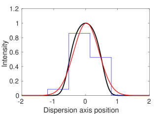
Figure 20: Example of the misfit of a pure Gaussian to the convolved projected circle. Thick black line: intrinsic convolved projected circle LSF; blue ‘histogram’ plot: the LSF sampled at 1.5 pixels/FWHM and pixel phase -0.29, which gives the maximum position bias error; red curve: the Gaussian which best fits the sampled data.

The above two LSFs are perfectly symmetrical, an ideal which is not achieved in practice, due to complex residual optical aberrations and other effects. These can give rise to fine structure in the LSF, which is of particular importance because LSF structure finer than the pixel scale will cause a shift in the fitted location of the feature, as it moves from contributing in one pixel to the next one. It is an example of the desirability of band limiting the data before sampling, which is not possible in this case. Thus the smoothing effect of integrating over pixels does not reduce this bias. The final LSF to be considered in this section is an example of the difference that some asymmetric fine structure can make to the bias errors. Figure 21 shows an LSF constructed by perturbing a Gaussian with three sinusoids, having spatial periods of 1, 0.5 and 0.25 $\times$ the FWHM. Figures 22 and 23 show the results. Compared with the fits to the pure Gaussian LSF in Figure 16 the bias errors in position are much larger (15$\times$ greater at sample frequency 1.5) and continue to much larger sampling frequencies, despite the perturbation of the Gaussian form being relatively minor. The bias errors in these Figures were computed relative to the unperturbed parent Gaussian, thus the zero points on the vertical scales are essentially arbitrary, and attention should be focussed on the range and variation of the errors. The flux (area) errors are not large, with the greatest being -1.8% at 2.1 pixels/FWHM.

In Figure 23 the same three sample frequencies are plotted as for the pure Gaussian case (Figure 17); it is notable that the position errors are much larger and do not decrease nearly as quickly as sample frequency increases. Thus the smoothness of the intrinsic (unsampled) LSF is an important criterion if accurate wavelengths are to be obtained from a spectrograph when using simple line fitting procedures.

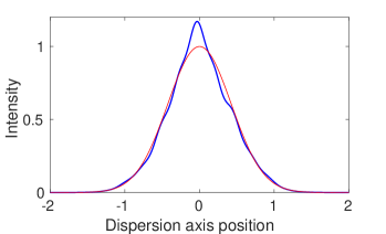
Figure 21: Thick blue curve - Gaussian LSF perturbed by some high-frequency noise. Thin red curve - the unperturbed parent Gaussian LSF. The perturbation is a sum of 3 sine curves with amplitudes $A_{i}=[0.1,0.05,0.03]$, pixel phases at sine wave zero crossing $\phi_{i}=[-0.33,0.85,-0.6]$ and frequencies $f_{i}=[1,2,4]$ where $f_{1}$ corresponds to one cycle across the FWHM. The final perturbed curve is a Gaussian of peak and FWHM = 1 multiplied by (1 + the sum of sine waves).

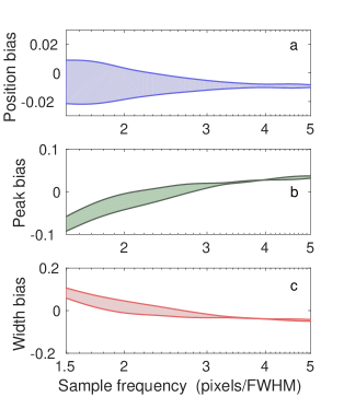
Figure 22: Bias errors of position, peak height and width for a plain Gaussian fitted to a perturbed Gaussian LSF. For position and width the errors are relative to the parent FWHM of 1.0, and the peak bias is relative to the parent Gaussian LSF peak = 1.0. The filled areas show the range of values covered by different pixel phases. The errors have been calculated relative to the original unperturbed LSF, and therefore have essentially arbitrary zero point offsets.

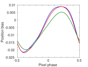
Figure 23: Bias errors of position as a function of pixel phase, for a plain Gaussian fitted to the perturbed Gaussian LSF. The blue curve is for sample frequency of 1.5 pixels/FWHM, red is at 1.6 and green at 1.9 pixels/FWHM.

7.3 Centroid position

The centroid (centre of gravity) of an isolated spectral feature is

$$C_{T}=\frac{\int_{-\infty}^{\infty}F(x)x\ dx}{\int_{-\infty}^{\infty}F(x)dx}$$ (13)

where $F(x)$ is the spectral intensity as a function of location $x$ along the dispersion axis, and $C_{T}$ represents the true centroid, i.e free from the effects of pixellation. This formula assumes that any background level has been subtracted, so the peak is sitting on zero background level. For pixellated data one has to use

$$C_{P}=\frac{\sum F_{i}x_{i}}{\sum F_{i}}$$ (14)

where the sum is over all pixels containing any part of the peak. The difference of these two expressions represents the bias of the pixellated centroid:

$$C_{P}-C_{T}=\frac{\int_{-\infty}^{\infty}F(x)(x_{i}-x)\ dx}{\int_{-\infty}^{\infty}F(x)dx}$$ (15)

where $x_{i}$ is the centroid of pixel $i$ which is nearest to the particular value of $x$. For pixels assumed to have uniform sensitivity, $x_{i}$ is the $x$ coordinate value at the centre of the pixel. The $(x_{i}-x)$ factor in this equation imparts a sawtooth characteristic to the integrand, which results in near-cancellation of the positive and negative parts. The overall result is further reduced by near cancellation of the contributions from the ascending and descending slopes of the LSF. The result is that centroid bias values can be very small under some circumstances. The bias results for some example LSFs will be considered below.

The principal advantage of the centroid is that it is model-independent, providing that it is clear where in the wings of the feature the summation should be truncated. The outstanding disadvantage is the centroid’s noise response. In the case of uniform noise of standard deviation $\sigma$ in each pixel, it can be shown that the variance of the pixellated centroid is given by

$$\sigma_{C_{P}}^{2}=\frac{\sigma^{2}}{(\sum F_{i})^{2}}\sum(x_{i}-C_{P})^{2},$$ (16)

which results in the variance increasing quadratically and without limit as more pixels are included in the wings of the feature. In this respect least squares fits to the LSF are obviously superior. However, the centroid is still of interest for the reasons given above, and in fact if the summation for centroid evaluation is suitably truncated, its noise need not be excessive: for example in the case of a Gaussian LSF the centroid noise given by equation 16 equals the 2-parameter least squares fit noise (equations 1 or 2) when the centroid summation includes 98 - 99 % of the flux.

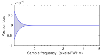
Figure 24: Bias error of centroid positions for a Gaussian LSF. The filled area shows the range covered by different pixel phases.

Figure 24 shows the centroid bias for the case of a Gaussian LSF. Bias is negligible at 2.0 pixels/FWHM, and even at 1.5 pixels/FWHM it reaches a maximum (at particular pixel phases) of only $7.05\times 10^{-5}$ of the FWHM. The behaviour as a function of pixel phase is shown in Figure 25, illustrating the near-sinusoidal form of the very small bias errors. The maximum bias is $14\times$ less than that shown in Figure 16 for the fit of a plain Gaussian to a Gaussian LSF, illustrating the bias-resistant nature of the centroid in this case.

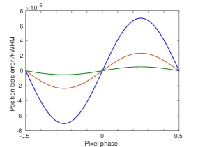
Figure 25: Bias errors of centroid position as a function of pixel phase for a Gaussian LSF. The largest amplitude curve (blue) is at 1.50 pixels/FWHM; the other two are at 1.594 and 1.715 pixels/FWHM.

For the convolved projected circle LSF the steeper sides and flattened top produce much larger errors, as shown in Figures 26 and 27. At 1.5 pixels/FWHM the maximum error is $9.24\times 10^{-3}$, i.e. $131\times$ greater than for the Gaussian LSF. Furthermore, there is a secondary maximum in the bias errors at 2.08 pixels/FWHM, where the largest error is $1.42\times 10^{-3}$.

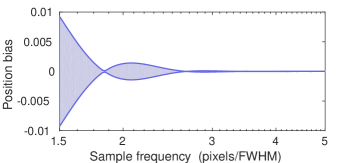
Figure 26: Bias error of centroid positions for the convolved projected circle LSF. The filled area shows the range covered by different pixel phases.

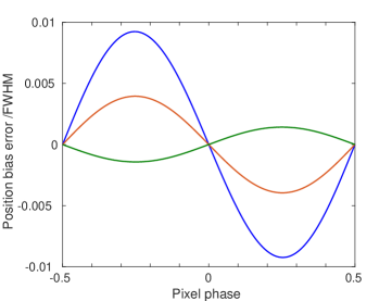
Figure 27: Bias errors of centroid position as a function of pixel phase for the convolved projected circle LSF. The largest amplitude curve (blue) is at 1.50 pixels/FWHM; the other two are at 1.653 and 2.083 pixels/FWHM.

The final LSF form considered here is the perturbed Gaussian, as shown in Figure 21. The result for its centroid bias as a function of sample frequency is shown in Figure 28. The errors are far larger than for the centroid of a pure Gaussian - with the maximum range of errors at 1.5 pixels/FWHM being $1.24\times 10^{-2}$, which is $88\times$ greater than the range for the pure Gaussian at the same sample frequency. This shows the great importance of high frequency distortion of the LSF for centroid bias. The presence of high frequency components in the LSF also produces (in this example) a secondary maximum in bias range at a sampling frequency as high as 4 pixels/FWHM, where the range is $2.4\times 10^{-3}$. Other tests (not shown) used an asymmetrical Gaussian, constructed from two half-Gaussians of equal peak height but unequal widths, joined at the peak: for FWHMs differing by a factor of 1.10 the centroid bias was $22\times$ greater than for the symmetrical Gaussian and for a width ratio of 1.44 the bias was $160\times$ greater (at 2 pixels/FWHM).

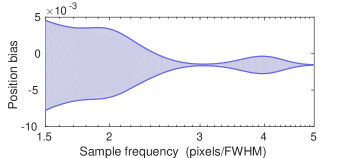
Figure 28: Bias error of centroid positions for the perturbed Gaussian LSF. The filled area shows the range covered by different pixel phases.

8 RESOLVING CLOSELY-SPACED FEATURES

The consistent scale of resolving power described in section 6 provides a quantitative measure which takes into account the effect of finite pixel widths. Nevertheless, users of pixellated spectra are likely to want further information regarding how much the pixellation affects the ability to distinguish two closely-spaced spectral lines. There are many ways one might quantify the effects of pixellation - for example the increase in flux or wavelength uncertainty of one spectral line as another draws closer. However, there are a large number of variable parameters and it is not clear that such results would be helpful. Perhaps the most basic property of resolved lines that an observer looks for is the presence of a relative minimum between the two peaks (in the case of emission lines). In this section, the effects of pixellation on such a relative minimum are examined.

Following the standard adopted in Paper 1, the criterion for two spectral features that are individually unresolved to be regarded as just resolved from each other is that there should be a relative minimum between the two (intrinsically equal) peaks that is 81.1% of the height of either peak. This is based on the Rayleigh criterion separation of two sinc² LSFs and has the advantage that the criterion itself is independent of the noise properties of the data. The procedure adopted was to first choose an LSF functional form and sampling frequency, and then place the first peak at the origin with a specified pixel phase. An iterative procedure was then used to find the separation of the two (intrinsic) peaks which results in the relative minimum of the sampled data being 81.1% of the height of the lower of the two sampled main peaks (they will in general be unequal due to the sampling). Figure 29 shows the results for Gaussian LSFs. The curves have a complex structure because changing the separation changes the pixel phase of the second peak, which in turn affects the desired separation if the pixellated second peak is the lower of the two. Changing separation also changes the contribution to the first peak from the wings of the second peak. The curves are not symmetric about zero pixel phase of the first peak because the second peak lies towards positive $x$ values and so contributes predominantly on that side. The horizontal grey line indicates the separation in the limit of fine sampling.

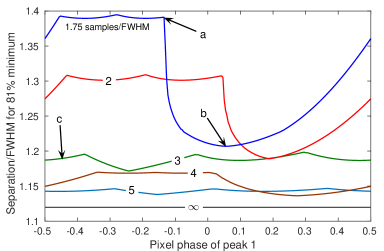
Figure 29: Illustration of the effects of pixellation on the ability to see two equal height Gaussian peaks as separate. The horizontal axis gives the pixel phase of the first of the two peaks. The vertical axis shows the separation of the two peaks that is required for there to be a local minimum in the pixellated data which is 81.1% of the lower of the two pixellated main peaks. Curves are given for sampling frequency values from 1.75 to 5 pixels/FWHM, as labelled. The horizontal grey line at separation/FWHM = 1.1196 is the limiting separation in the case of finely sampled LSFs. The points labelled ‘a’,‘b’,‘c’ refer to sample frequencies and pixel phases whose LSFs are shown in Figure 30.

Figure 30 shows the intrinsic and pixellated LSFs for the three cases pointed out in Figure 29. It is clear why a larger separation is needed in case ‘a’ than in case ‘b’ to maintain the 81.1% relative minimum. The structure of the minimum separation curves is one illustration of the complex non-linear effects which are introduced by sampling. Even at 2 pixels/FWHM there is a substantial (10.1%) variation of the critical separation with pixel phase, which may be compared with the far smaller (0.6%) range for the resolving power based on wavelength accuracy for the same LSF and sampling frequency as shown in Figure 15. This is due to the different resolution criteria employed in the two cases.

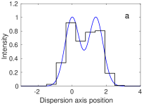
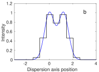
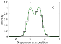
Figure 30: LSF plots for the three cases indicated in Figure 29

A corresponding calculation (not shown) was carried out for the convolved projected circle LSF. It gave results that are qualitatively similar to those of the Gaussian in Figures 29 and 30 although with smaller critical separations as a multiple of the FWHM.

9 THE FOURIER VIEW OF SAMPLING

9.1 Overview

The performance of optical imaging systems is often quantified using the Optical Transfer Function (OTF), which is the normalised Fourier Transform of the Point Spread Function (PSF). The modulus of the OTF is known as the Modulation Transfer Function (MTF) and gives a direct measure of a system’s ability to transmit fine detail from object to image. As well as giving an insight into performance of a subsystem, the MTF has the useful property that for successive components of an imaging system (e.g. atmosphere, optics, detector) the final MTF is the product of the component MTFs, provided that the transfers between the subsystems are incoherent.

The process of sampling of a function on a regularly-spaced grid naturally lends itself to a study through the use of Fourier methods, since there is a maximum spatial frequency to which the sampling can respond. It is well-known that of the Fourier components making up a function (here a 1-dimensional spectrum), any with spatial frequencies higher than the Nyquist limit of 2 samples per cycle will be aliased and thus incorrectly ascribed to a lower frequency. This section will examine the implications. An important simplification in this analysis is that to the extent that the LSF is constant over a region of a spectrum, that spectrum can be regarded as the convolution of the intrinsic spectrum with the LSF (with noise added after convolution). Thus it will suffice to examine the Fourier properties of the LSF instead of full spectra.

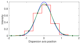
Figure 31: Illustration of the effects of sampling. Blue: Gaussian intrinsic LSF, with FWHM = 1 and peak = 1; red histogram-style line: the LSF sampled at 2 pixels/FWHM and pixel phase = 0.25; black diamonds: the sampled points; green: the intrinsic LSF convolved with the pixel rectangle.

Figure 31 illustrates the process by which a continuous LSF is rendered as a sequence of separated samples. It also shows the broadening effect of pixel convolution - in that the green line showing the intrinsic LSF convolved with the pixel rectangle passes exactly through the black sample points. Thus instead of summing the LSF across the width of each pixel, an exactly equivalent process is to convolve the LSF with the pixel rectangle and then point sample it at the centres of the nominal pixels. In the illustrated case at a sampling frequency of 2 pixels/FWHM, the convolved LSF has a FWHM 1.060 $\times$ greater than the intrinsic LSF, due to the effects of pixel smoothing.

A notable complication in using the MTF to study sampling is that an assumption underpinning the use of the MTF is that the process (in the present case, the formation of the observed spectrum from convolution of the ideal spectrum with the LSF) should be linear and shift-invariant. But the form of the sampled LSF depends on the pixel phase, so the process is not shift invariant. It is nevertheless still possible to derive some useful insight from Fourier methods. In particular, as pointed out by e.g. Hamming (1983), sin and cos are the eigenfunctions of equally spaced sampling. A sinusoidal function will be rendered with the correct functional form, amplitude and phase provided the sampling frequency is above the Nyquist limit of 2 samples per cycle. Since the MTF treatment considers an LSF as made up of sinusoidal Fourier components, sampling is expected to cause no errors for components below the Nyquist frequency, provided that they have not been corrupted by aliased components from above the Nyquist frequency. The results in the present work support that conclusion.

9.2 Fourier Transforms of LSFs

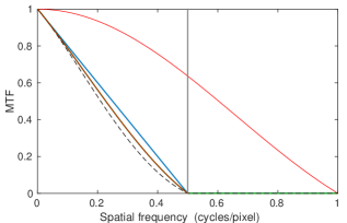
Figure 32: Modulation Transfer Function of a sinc² LSF, sampled at 1.7718 pixels/FWHM. In order to obtain good accuracy of the transform, the sinc² subsidiary lobes were included out to $\pm 100\times$FWHM. The first set of computations used 4096 points over this range, giving a well-sampled transform; the horizontal axis was then rescaled to show the results for a sampling frequency of 1.7718 pixels/FWHM. This is the reason that frequencies above the Nyquist frequency of 0.5 cycles/pixel can be shown. Red curve: sinc function due to smoothing by contiguous pixels of uniform sensitivity; blue straight line: the transform of the sinc² LSF; brown line: product of the above two, showing the MTF of the sampled LSF; grey vertical line: the Nyquist frequency for sampling; black dashed line: the LSF transform multiplied by two sinc factors (see text). Not visible in the plot are 6 additional lines, all coincident with the brown line. They were computed by actually sampling the sinc² LSF at 1.7718 pixels/FWHM and 6 different pixel phases, and then Fourier Transforming.

The first case considered, shown in Figure 32, is for a sinc² LSF. It is well known that the Fourier Transform of a sinc function is a rectangle, while that of a sinc² function is a triangle peaked at the origin (e.g. Bracewell 1978). The FWHM of

$${\rm sinc}^{2}(x)=\bigg{(}\frac{\sin(\pi x)}{\pi x}\bigg{)}^{2}$$ (17)

is 0.88589, and its Fourier Transform is band-limited to frequencies less than 1. Hence a sinc² function with FWHM = 1.77178 pixels has a transform band-limited to frequencies less than 0.5 cycles/pixel, i.e. the Nyquist frequency for sampling. In Figure 32 the straight blue line shows the normalised Fourier Transform of sinc², when sampled at the Nyquist frequency. The red curve which reaches zero at twice the Nyquist frequency is a sinc function which represents the effect of pixel convolution on the spatial frequencies (since sinc is the Fourier Transform of the rectangle representing uniform pixel sensitivity). It reaches a null at one cycle per pixel, where pixel smoothing would result in zero modulation transfer. The brown curve shows the product of these two functions, i.e. the MTF of a sinc² LSF sampled by contiguous rectangular pixels of uniform sensitivity, at 1.7718 samples/FWHM. (These three curves were computed using fine sampling and then rescaling the horizontal axis.)

The dashed curve relates to the statement (e.g. Boreman (2001), Fischer et al. (2008)), that in addition to the sinc factor due to convolution with the rectangular pixels, there is another identical sinc factor from the sampling process itself, due to ‘sample scene phase averaging’. But after convolving the LSF with the pixel rectangle, the sampling is then done at points representing the centres of pixels. Thus there is no additional convolution with a rectangle, and no further sinc factor in the MTF. This is demonstrated in Figure 32 because the brown curve also includes 6 Fourier Transforms of the LSF actually sampled at 1.7718 samples/FWHM. There is no dependence on pixel phase, and all transforms match the expectation that one sinc factor is appropriate. This conclusion is supported by the analysis of Yaroslavsky (2013).

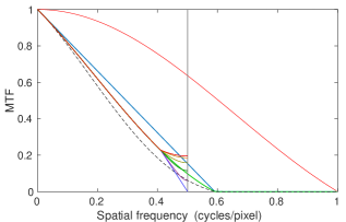
Figure 33: Modulation Transfer Function of a sinc² LSF, sampled at 1.5 pixels/FWHM. Otherwise as for Figure 32. In this case the curves for the 6 different pixel phases diverge sharply at spatial frequencies where aliasing occurs. (The latter curves must terminate at the Nyquist frequency because they were computed by actually sampling at 1.5 pixels/FWHM.)

To illustrate the utility of the frequency approach, Figure 33 shows again the MTF of a sinc² LSF, but this time undersampled at 1.5 pixels/FWHM. The maximum spatial frequency of the LSF is now 0.5906 cycles/pixel, so frequencies between 0.5 and 0.5906 are aliased, with their Fourier components folded back into the range 0.4094 - 0.5. It is precisely in this range that the 6 curves for different pixel phases diverge from the mean. This demonstrates that pixel phase dependence occurs only for spatial frequencies corrupted by aliased signal: for uncorrupted frequencies the amplitude of a Fourier component is correctly measured irrespective of pixel phase, so the MTF, which measures the relative amplitude of components, is unaffected. Figure 5 shows that the same applies for $\sigma_{\lambda}$ as a function of sampling frequency - all pixel phases give the same result until aliasing begins at low sample rates. This behaviour is as expected since sinusoids are the eigenfunctions of equally spaced sampling.

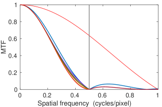
Figure 34: Modulation Transfer Function of the convolved projected circle LSF, sampled at 2 pixels/FWHM. The colour coding of curves is as for Figures 32 and 33. For this sampling frequency and LSF shape there is a null at 0.498, i.e. near the Nyquist frequency.

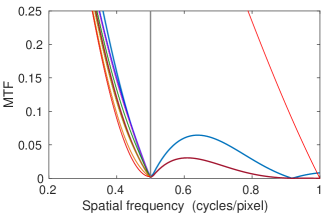
Figure 35: Enlarged view of the lower part of Figure 34, showing more clearly the curves for 6 different pixel phases.

The above discussion of the sampling MTF for a sinc² LSF has illustrated important points, but in order for the sinc² function to properly exhibit its band-limited nature, a large number of subsidiary lobes were included in the evaluations. This is quite unrealistic for astronomical spectra, where noise and complex structure limit the effective LSF to the main lobe only. Thus as a final example, the MTF of the convolved projected circle LSF is shown in Figures 34 and 35. As expected, the steep sides of this LSF (even after convolution with a Gaussian) result in substantial high spatial frequency components and at the sampling frequency of 2 pixels/FWHM there is considerable amplitude beyond the Nyquist limit. The aliasing of these components results in the curves for the 6 different pixel phases being distinct over most of the observable spatial frequency range. This is consistent with the $\sigma_{\lambda}$ curves of Figure 6 which show pixel-phase dependence over essentially the entire sample frequency range plotted.

10 MISCELLANEOUS COMPLICATIONS

10.1 Non-uniform pixel sensitivity

The results described above assumed that each pixel has uniform sensitivity which drops sharply to zero at the pixel boundary, i.e. the pixel response as a function of position is a rectangular function. This ideal shape will not be achieved in practice - the response may drop off towards the edges of the pixel, possibly in an asymmetric fashion, and in thick CCD chips there may be charge diffusion which leads to some response to photons which actually arrived in adjacent pixels (Widenhorn et al.2010). Jorden et al.(1994) used a small-diameter light spot to measure the intrapixel sensitivity variations of a number of CCDs and found variations of order 10%. Barron et al.(2007) used a similar technique to measure sub-pixel sensitivity variations in a number of near-IR detectors and found high QE detectors had less than 2% variation, while moderate QE devices showed strong asymmetric intrapixel structure. Departures from ideal performance of thick chips were discussed by Stubbs (2014).

Lauer (1999b) examined this issue for the case of undersampled HST images, and showed how to construct maps of intrapixel sensitivity variations. His analysis used a set of dithered images which allow the effective PSF (i.e. the optical PSF convolved with the pixel response function) to be obtained with fine sampling. (This is essentially the same process as used here to create the AAOmega LSF in Figure 8.)

Intrapixel variations can be expected to cause minor departures of the actual $\sigma_{\lambda}$ curves from those illustrated in Figures 1 to 9, which are in any case intended only as illustrations of some possible forms. More important in practice is the accurate determination of the effective LSF. Sensitivity loss at the edge of each pixel and/or leakage from adjacent pixels would smooth out the abrupt change of signal from one pixel to the next as the illumination peak moves - hence the ‘quad-cell’ effect which resulted in low $\sigma_{\lambda}$ for pixel phase 0.5 in Figures 1, 3 and 5 would be diminished and the local maximum in $\sigma_{\lambda}$ may not occur (e.g. Spinhirne et al 1998). Note that the ‘effective LSF’, i.e. the instrumental LSF convolved with the pixel response as found in Figure 8, automatically includes the effects of any departure of the pixel response from the ideal rectangular function $-$ without those departures being known explicitly.

Intrapixel sensitivity variations can be expected to have a significant effect on position bias errors, if they interact with high spatial frequency substructure of the optical LSF. For any given system detailed measurements would be needed to quantify the effects.

A more subtle issue is the non-linear response known as the ‘brighter-fatter’ effect, whereby accumulated charge affects the apparent width of pixels, leading to bright objects appearing to be up to a few percent wider than faint objects (Antilogus 2014; Rasmussen 2014; Guyonnet 2015). However, the pixel sampling frequency is not of particular importance in that case.

10.2 Dithering and non-contiguous pixels

While detectors with contiguous pixels represent the most common case, it is also appropriate to examine what happens when the pixel spacing is not equal to the pixel width. The spacing is less than the width when dithered (sub-stepped) exposures are combined, while the spacing would be greater than the width for sparse arrays. In all cases, the process can be considered as convolution of the intrinsic LSF with the pixel response (i.e. convolution with the pixel width) and then point sampling at the appropriate spacing, which is less than the width for dithering, equal to the width for contiguous pixels, or greater than the width for sparse arrays. The use of dithering in improving undersampled images, particularly those from HST, has been studied by many authors, e.g. Lauer (1999a; 1999b), Bernstein (2002), Fruchter and Hook (2002), Fruchter (2011) and Boreman (2001). Lauer noted that for accurate reconstruction of a sampled function, it must be band-limited, i.e. it should avoid corruption of Fourier components by aliasing.

The MTF is useful in showing the effects of varying the sampling rate in this way. For example, Figure 36 shows the MTF of the convolved projected circle LSF sampled at 2 pixel widths per FWHM as in Figure 34, but with the data combined with a second exposure offset by half a pixel width, so that the final pixel spacing is half of the pixel width. This results in 4 pixel spacings per FWHM. The horizontal axis shows spatial frequencies from 0 to 1 cycle per pixel width; with dithering this is equivalent to 0 to 0.5 cycles per pixel spacing. Since the Nyquist frequency is related to sampling, not pixel convolution, the entire range shown in Figure 36 is below the Nyquist frequency. Comparison of the two Figures shows the benefit of dithering: the second lobe of the LSFs MTF, which lay beyond the Nyquist frequency without dithering, is now correctly sampled. As a result, there is negligible corruption due to aliasing and negligible dependence on pixel phase. This is an example of an LSF which has significant high spatial frequency content, and benefited from sub-stepping to reduce the pixel spacing.

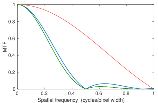
Figure 36: Modulation Transfer Function of the convolved projected circle LSF, sampled at 2 pixel widths per FWHM and dithering with pixel spacing = 0.5 $\times$ pixel width. The colour coding of curves is as for Figures 32 and 33. The green line shows 6 coincident lines for different pixel phases.

10.3 Poisson noise

The above examinations of systematic bias errors, separation of closely spaced features and the Fourier picture are independent of the noise characteristics of the data, but the treatment of wavelength, width and peak errors in Sections 3, 4 and 5 and the consistent resolving power scale in Section 6 do assume noise that is constant across pixels. This is suitable for weak emission or absorption lines on a spectral continuum level, or any spectrum where detector noise dominates. However, for strong features where Poisson shot noise from the observed object dominates, the assumption of constant noise can be only an approximation. It is therefore appropriate to examine briefly the differences in the case of Poisson noise.

The discussion will be limited to the case of a Poisson noise dominated unresolved emission peak sitting on zero background level. This would describe strong emission features in a spectrum. Since the Poisson noise approaches zero as the LSF intensity drops in the wings of the profile, there is no need to make a least-squares fit of the LSF to the data in order to find the location (wavelength). Instead, the centroid can be used directly. In the limit of fine sampling of a Gaussian peak the RMS centroid error is given by the simple formula:

$$\sigma_{\lambda}=\frac{\sigma_{\rm G}}{\surd N}$$ (18)

where $\sigma_{\rm G}$ is the FWHM/2.3548 of the Gaussian LSF and $N$ is the total number of photon counts in the peak. This is the same as the formula for the standard error of the mean of a Gaussian statistical distribution. When the peak has been split into finite-width pixels, the equation for the variance of the centroid is

$$\sigma_{C_{P}}^{2}=\frac{1}{N^{2}}\sum F_{i}(x_{i}-C_{P})^{2}.$$ (19)

where $F_{i}$ is the count in pixel $i$ located at $x_{i}$ and $C_{P}$ is the position of the pixellated centroid. This expression is often used in the context of the position uncertainty of the image spots formed by a Shack-Hartmann wavefront sensor (e.g. Rousset 1999). It has been used here to evaluate the RMS centroid uncertainty as a function of sampling frequency, as shown in Figure 37. This may be compared with Figure 1 which shows the same for constant (normally-distributed) noise. Although the two Figures show a broadly similar increase of wavelength uncertainty for coarser sampling, it is notable that in the Poisson case there is much less dependence on pixel phase, with minimal separation of curves at different pixel phase even at 1.5 pixels/FWHM. The maximum enhancement of the RMS error over the fine-sampling limit is only $1.098\times$, as compared with the range $1.093-1.235\times$ for constant noise.

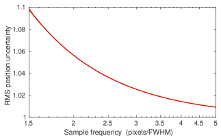
Figure 37: Wavelength uncertainty vs sampling frequency for a Gaussian LSF subject to Poisson noise. The position (wavelength) is taken from the centroid of the observed LSF. The full range of pixel phases is shown as 6 curves, but they are coincident except for minor differences near 1.5 pixels/FWHM. The curves have been normalised to unity at very large sample frequency.

Finding the parameters of such a pixellated Poisson-dominated peak is equivalent to fitting a histogram from a counting experiment in the particle physics context, and formulas for the bias, variance and skewness of the distribution of any parameter derived from such data were given by Eadie et al.(1971).

11 CONCLUSIONS

There are a number of consequences of sampling spectra into pixels, and this paper is intended to illustrate the principal effects which are of concern to the end-users of such sampled data. In summary:

1) Random noise errors in wavelength are increased by sampling (Section 3). Uncertainties are typically $\sim 10-20$% worse at a sample frequency of 2 pixels/FWHM but depend on the functional form of the Line Spread Function (LSF). The important case of the projected circle convolved with a Gaussian (representing a projected multi-mode fibre with some spectrograph aberrations) shows strong dependence on the pixel phase (i.e. the position of a spectral feature with respect to the pixel centre), with uncertainties increased by 20% at 2 pixels/FWHM and certain pixel phases.

2) If the width of a spectral feature is to be determined, the effects of pixellation on random noise errors are considerably more severe than for wavelength (Section 4), especially below 2 pixels/FWHM, and they are strongly dependent on pixel phase.

3) Pixellation causes only a minor increase in the random noise of the fitted peak amplitude of an unresolved spectral feature (Section 5). Increases of 5% or less at 2 pixels/FWHM are to be expected, but with some dependence on pixel phase.

4) Pixellation tends to smooth out the relative minimum between two closely spaced emission lines (or equivalently, the relative maximum between two absorption lines). If one wishes to see a relative minimum of 81% of the peak (equal to the Rayleigh criterion separation for two finely-sampled sinc² LSFs) then the separation required is significantly increased by sampling, but in a complex manner due to the effects of pixel phase (Section 8).

5) As demonstrated in Robertson (2013; Paper 1), the FWHM is a poor measure of spectral resolution, when LSFs of different form need to be compared. In Section 6 the method for calculating resolving power on a consistent scale based on wavelength accuracy is extended from that given in Paper 1 to include effects of pixellation.

6) Pixellation of spectra can produce systematic bias errors in wavelength that depend on pixel phase and the method of wavelength determination, but are not reduced by high signal/noise data. As shown in Section 7 such errors may be negligible for well-sampled symmetric LSFs. But they are greatly increased by asymmetry in the LSF and/or high spatial frequency components that are not adequately sampled by the detector. Thus any fine structure in the intrinsic LSF (i.e. the unsampled image as it falls on the detector plane) will have a significant role in producing wavelength bias errors, and a smooth symmetrical PSF that varies at most slowly across the detector is desirable for high precision work.

7) The Modulation Transfer Function (MTF; normalised amplitude of the Fourier Transform of the LSF) can show the extent to which spatial frequencies making up the LSF are aliased due to inadequate sampling frequency. Any Fourier component which is aliased will then corrupt another component which is below the Nyquist frequency and would have otherwise been correctly recorded. Pixel-phase dependence develops for spatial frequencies that have been corrupted by aliased signal from above the Nyquist frequency.

8) There has developed in the literature a practice of referring to a sampling frequency of 2 samples per FWHM as being the Nyquist limit. This is incorrect, since it is not the same as 2 samples per cycle of a sinusoid, and most common LSFs have aliased high frequency components when sampled at 2 pixels/FWHM. Nevertheless, it is true that for most LSF forms resulting from spectrographs, 2 samples/FWHM is a reasonable minimum if high precision is not required. In the case of a diffraction-limited slit input, 2 samples/FWHM is slighly more than needed to avoid any aliasing (but this assumes that subsidiary lobes of the diffraction pattern can be included in the analysis - which is unlikely in spectra with noise and many features). For high precision work with typical non-diffraction-limited LSFs, a larger sampling frequency should be used. For example Chance et al.(2005) recommend 4.5 $-$ 6.5 pixels/FWHM of a Gaussian LSF after pixel convolution to avoid any significant aliasing, and the HARPS planet-finder spectrograph (Mayor et al, 2003) uses 3.2 pixels/FWHM.

9) A recommendation from this work is that it is desirable for designers of spectrographic instruments to carry out simulations using computed LSFs (suitably smoothed to remove spurious high frequency features such as from a finite number of rays traced, but retaining all ‘real’ fine structure). Then the extent to which noise in parameter estimates is increased, the amount of pixel-phase dependence and the bias errors can be found for any proposed camera speed and detector pitch.

10) For instruments where the end users have choices regarding sampling frequency (e.g. from on-chip binning, or different spectrograph configurations) it is highly desirable that the instrument team should carry out simulations using the actual LSF and so provide in the user manual data regarding the effects on noise, bias, separation of peaks, pixel-phase dependence etc. which can aid the user in deciding which configuration to use.

REFERENCES

Anderson, J. and King, I.R. PASP 112, 1360, 2000.
Antilogus, J., Astier, P., Doherty, P., Guyonnet, A, and Regnaulta, N. Inst. 9, C03048 2014.
Barron, N., Borysow, M., Beyerlein, K., Brown, M., Lorenzon, W., Schubnell, M., Tarle´, G.,
Tomasch, A. and Weaverdyck, C. PASP 119 466 2007.
Bernstein, G. PASP 114, 98, 2002.
Bickerton, S.J. and Lupton, R.H. MNRAS 431, 1275, 2013.
Boreman, G.D. Modulation Transfer Function in Optical and Electro-Optical Systems SPIE
Press 2001.
Bracewell, R.N. The Fourier Transform and its Applications McGraw-Hill 1978.
Bracewell, R.N. Two Dimensional Imaging, Prentice Hall p365, 1995.
Chance, K., Kurosu, T.P. and Sioris, C.E. Appl. Opt. 44, 1296 2005.
Clarke, T.W., Frater, R.H., Large, M.I., Munro, R.E.B. and Murdoch,
H.S. Aust. J. Phys. Astrophys. Suppl. 10, 3, 1969.
Eadie, W.T., Dryard, D., James, F.E., Roos, M. and Sadoulet, B. Statistical Methods in
Experimental Physics North-Holland p. 146, 1971.
Fischer, R.E., Tadic-Galeb, B. and Yoder, P.R. Optical System Design McGraw-Hill 2008.
Fruchter, A.S. PASP 123, 497, 2011.
Fruchter, A.S. and Hook, R.N. PASP, 114, 144, 2002.
Guyonnet, A., Astier, P., Antilogus, P., Regnault, N. and Doherty, P. Astron. Astrophys. 575,
A41 2015.
Hamming, R.W. Digital Filters Prentice-Hall 2nd ed, p30, 1983.
Jorden, P.R., Deltorn, J-M and Oates, A.P. Proc. SPIE 2198, 836, 1994.
Lauer, T.R. PASP 111, 227, 1999a.
Lauer, T.R. PASP 111, 1434, 1999b.
Mayor, M. et al. ESO Messenger 114, 20, 2003.
Rasmussen, A. J. Inst 9, C04027 2014.
Robertson, J.G. PASA 30, e048 2013 (Paper 1).
Rousset, G. in Adaptive Optics in Astronomy ed. Roddier, F. Cambridge University Press p
115, 1999.
Saunders, W., Bridges, T., Gillingham, P., Haynes, R., Smith, G.A., Whittard, J.D.,
Churilov, V., Lankshear, A., Croom, S., Jones, D. and Boshuizen, C. SPIE 5492, 389, 2004.
Saunders, W. Proc. SPIE 9147 60 2014.
Spinhirne, J.M., Allen, J.G., Ameer, G.A., Brown, J.M., Christou, J.C., Duncan, T.S., Eager,
R.J., Ealey, M.A., Ellerbroek, B.L., Fugate, R.Q., Jones,G.W., Kuhns, R.M., Lee, D.J., Lowrey,
W.H., Oliker, M.D., Ruane, R.E., Swindle, D.W., Voas, J.K., Wild, W.J., Wilson, K.B. and John
L. Wynia, J.L. Proc. SPIE 3353, 22, 1998.
Stubbs, C.W. J. Inst. 9, C03032, 2014.
Vollmerhausen, R.H., Reago, D.A. and Driggers, R.G. Analysis and Evaluation of Sampled
Imaging Systems SPIE Press 2010.
Widenhorn, R., Alexander Weber-Bargioni, A., Blouke, M.M., Bae, A.J. and Bodegom, E.
Opt. Eng. 49, 044401, 2010.
Yaroslavsky, L.P. Theoretical Foundations of Digital Imaging using MATLAB CRC Press p83
2013.