Balian-Low type theorems in finite dimensions

Abstract.

We formulate and prove finite dimensional analogs for the classical Balian-Low theorem, and for a quantitative Balian-Low type theorem that, in the case of the real line, we obtained in a previous work. Moreover, we show that these results imply their counter-parts on the real line.

1. Introduction

1.1. A Balian–Low type theorem in finite dimensions.

Let $g\in L^{2}(\mathbb{R})$. The Gabor system generated by $g$ with respect to the lattice $\mathbb{Z}^{2}$ is given by

$$G(g)=\{e^{2\pi int}g(t-m)\}_{(m,n)\in\mathbb{Z}^{2}}.$$ (1)

The classical Balian-Low theorem [3, 4, 9, 21] states that if the Gabor system $G(g)$ is an orthonormal basis, or a Riesz basis, in $L^{2}(\mathbb{R})$, then $g$ must have much worse time-frequency localization than what the uncertainty principle permits. The precise formulation is as follows (see [7] for a detailed discussion of the proof and its history).

Theorem A (Balian, Battle, Coifman, Daubechies, Low, Semmes).

Let $g\in L^{2}(\mathbb{R})$. If $G(g)$ is an orthonormal basis or a Riesz basis in $L^{2}(\mathbb{R})$, then

$$\int_{\mathbb{R}}|t|^{2}|g(t)|^{2}\mathrm{d}t=\infty\quad\textrm{or}\quad\int_{\mathbb{R}}|\xi|^{2}|\hat{g}(\xi)|^{2}\mathrm{d}\xi=\infty.$$ (2)

We note that by Parseval’s identity, condition (2) is equivalent to saying that we must have either

$$\int_{\mathbb{R}}|\hat{g}^{\prime}(\xi)|^{2}\mathrm{d}\xi=\infty\quad\textrm{or}\quad\int_{\mathbb{R}}|{g}^{\prime}(t)|^{2}\mathrm{d}t=\infty.$$ (3)

That is, these integrals are considered infinite if the corresponding functions are not absolutely continuous, or if they do not have a derivative in $L^{2}$.

In the last 25 years, the Balian-Low theorem inspired a large body of work in time-frequency analysis, including, among others, a non-symmetric version [6, 12, 13, 23], an amalagam space version [19], versions which discuss different types of systems [10, 17, 18, 23], versions not on lattices [8, 16], and a quantified version [24]. The latter result will be discussed in more detail in the second part of this introduction.

Although it provides for an excellent “rule of thumbs” in time-frequency analysis, the Balian–Low theorem is not adaptable to many applications since, in realistic situations, information about a signal is given by a finite dimensional vector rather than by a function over the real line. The question of whether a finite dimensional version of this theorem holds has been circling among researchers in the area. In particular, Lammers and Stampe pose this as the “finite dimensional Balian-Low conjecture” in [20]. Our main goal in this paper is to answer this question in the affirmative.

Let $N\in\mathbb{N}$ and denote $d=N^{2}$. We consider the space $\ell_{2}^{d}$ of all functions defined over the cyclic group $\mathbb{Z}_{d}:=\mathbb{Z}/d\mathbb{Z}$ with the normalization,

$$\|b\|_{d}=\frac{1}{N}\sum_{j=0}^{d-1}|b(j)|^{2}\qquad b=\{b(j)\}_{j=0}^{d-1}.$$ (4)

To motivate this normalization, let $g$ be a continuous function in $L^{2}(\mathbb{R})$ and put $b(j)=g({j}/{N})$, $j\in\mathbb{Z}\cap[-N^{2}/2,N^{2}/2)$. That is, the sequence $b\in\ell_{2}^{d}$ consists of samples of the function $g$, at steps of length ${1}/{N}$ over the interval $[-N/2,N/2]$. Then, for “large enough” $N$, the above $\ell^{2}$ norm can be interpreted as a Riemann sum approximating the $L^{2}(\mathbb{R})$ norm of $g$. Note that in Section 2, we define the finite Fourier transform $\mathcal{F}_{d}$ so that it is unitary on $\ell_{2}^{d}$.

Let $N\mathbb{Z}_{d}$ denote the set $\{Nk:k\in\mathbb{Z}\}$ modulo $d$. For $b\in\ell_{2}^{d}$, the Gabor system generated by $b$ with respect to $(N\mathbb{Z}_{d})^{2}$, is given by

$$G_{d}(b):=\{e^{2\pi i\frac{\ell j}{d}}b(j-k)\}_{(k,\ell)\in(N\mathbb{Z}_{d})^{2}}.$$ (5)

We point out that, with the choice $b(j)=g(j/N)$, the discrete Gabor system $G_{d}(b)$ yields a discretization of the Gabor system $G(g)$ restricted to the interval $[-N/2,N/2)$.

To formulate the Balian-Low theorem in this setting, we use a discrete version of condition (3). To this end, we denote the discrete derivative of a function $b=\{b(j)\}_{j=0}^{d-1}\in\ell_{2}^{d}$ by

$$\Delta b:=\Big{\{}b(j+1)-b(j)\Big{\}}_{j=0}^{d-1},$$

and put

$$\alpha(N)=\inf\{\|{N}{\Delta b}\|_{d}^{2}+\|{N}{\Delta(\mathcal{F}_{d}b)}\|_{d}^{2}\},$$ (6)

where the infimum is taken over all sequences $b\in\ell_{2}^{d}$ for which the system $G_{d}(b)$ is an orthonormal basis in $\ell_{2}^{d}$. We note that for the choice $b(j)=g(j/N)$, samples of the derivative of $g$ at the points ${j}/{N}$ are approximated by $N\Delta b$. Therefore, the expression inside of the infimum is a discretization of the integrals in the condition (3). Our finite dimensional version of the Balian-Low theorem, that answers the finite Balian-Low conjecture in the affirmitive, may now be formulated as follows.

Theorem 1.1.

There exist constants $c,C>0$ so that, for all integers $N\geq 2$, we have

$$c\log N\leq\alpha(N)\leq C\log N.$$

In particular, $\alpha(N)\rightarrow\infty$ as $N$ tends to infinity.

Remark 1.2.

Theorem 1.1 also holds in the case that the infimum in $\alpha(N)$ is taken over all $b\in\ell_{2}^{d}$ for which the system $G_{d}(b)$ is a basis in $\ell_{2}^{d}$ with lower and upper Riesz basis bounds at least $A$ and at most $B$, respectively. In this case, the constants $c,C$ in Theorem 1.1 depend on $A$ and $B$. (For a precise definition of the Riesz basis bounds see Section 2). The dependence on the Riesz basis bounds is necessary, in the sense that it can not be replaced by a dependence on the $\ell_{2}^{d}$ norm of $b$ (see Remark 4.3).

Remark 1.3.

The classical Balian-Low theorem (Theorem A) follows as a corollary of Theorem 1.1, as we show in Section 6.

Remark 1.4.

By restricting to $N\geq N_{0}$, for large $N_{0}$, the constants in the above theorem improve. Indeed, combining Proposition 4.1 with Remark 4.4, we have

$$\lim_{N_{0}\rightarrow\infty}\Big{(}\inf_{N\geq N_{0}}\frac{\alpha(N)}{\log N}\Big{)}\geq\frac{1}{4\log 2},$$

while combining the same proposition with Remark 4.6 yields the asymptotic bound

$$\lim_{N_{0}\rightarrow\infty}\Big{(}\sup_{N\geq N_{0}}\frac{\alpha(N)}{\log N}\Big{)}\leq 16\pi^{2}.$$

1.2. A finite dimensional quantitative Balian–Low type theorem.

In [22], F. Nazarov obtained the following quantitative version of the classical uncertainty principle: Let $g\in L^{2}(\mathbb{R})$ and $\mathfrak{Q},\mathfrak{R}\subset\mathbb{R}$ be two sets of finite measure, then

$$\int_{\mathbb{R}\setminus\mathfrak{Q}}|g(t)|^{2}\mathrm{d}t+\int_{\mathbb{R}\setminus\mathfrak{R}}|\hat{g}(\xi)|^{2}\mathrm{d}\xi\geq De^{-C|\mathfrak{Q}||\mathfrak{R}|}\|g\|_{L^{2}(\mathbb{R})}^{2}.$$

In [24], we obtained the following quantitative Balian-Low theorem, which is a modest analog of Nazarov’s result for generators of Gabor orthonormal bases and, more generally, Gabor Riesz bases.

Theorem B (Nitzan, Olsen).

Let $g\in L^{2}(\mathbb{R})$. If $G(g)$ is an orthonormal basis or a Riesz basis then, for every $Q,R>1$, we have

$$\int_{|t|\geq Q}|g(t)|^{2}\mathrm{d}t+\int_{|\xi|\geq R}|\hat{g}(\xi)|^{2}\mathrm{d}\xi\geq\frac{C}{QR},$$ (7)

where the constant $C>0$ depends only on the Riesz basis bounds of $G(g)$.

This quantitative version of the Balian-Low theorem implies the classical Balian-Low theorem (Theorem A), as well as several extensions of it, including the non-symmetric cases and the amalgam space cases referred to above. Here, we prove the following finite dimensional version of this theorem.

Theorem 1.5.

There exists a constant $C>0$ such that the following holds. Let $N\geq{200}$, and let $b\in\ell_{2}^{d}$ (where $d=N^{2}$) be such that $G_{d}(b)$ is an orthonormal basis in $\ell_{2}^{d}$. Then, for all positive integers $Q,R\in[1,N/{16}]$, we have

$$\frac{1}{N}\sum_{j=NQ}^{d-1}|b(j)|^{2}+\frac{1}{N}\sum_{k=NR}^{d-1}|\mathcal{F}_{d}b(k)|^{2}\geq\frac{C}{QR}.$$

Remark 1.6.

Theorem 1.5 holds for general bases as well. In this case, the constant $C$, as well as the conditions on the sizes of $N$, $Q$ and $R$, depend on the Riesz basis bounds. This more general version of Theorem 1.5 is formulated as Theorem 5.3 in Section 4. (For a precise definition of the Riesz basis bounds see Section 2).

Remark 1.7.

As we show in Section 6, the quantitative Balian-Low theorem (Theorem B) follows as a corollary of Theorem 1.5.

Remark 1.8.

The conditions appearing in Theorem 1.5 are not optimal, but rather, these conditions were chosen to avoid a cumbersome presentation. In particular, we point out that a more delicate estimate in Lemma 5.1, or the use of a different function, will improve the condition $N\geq 200$. Some modifications in the proof of Lemma 5.2 will improve this condition as well. In addition, a careful analysis of the proof will allow one to improve each one of the conditions $N\geq 200$ and $Q,R\leq N/16$ at the expense of making the constant $C$ smaller. In fact, any two of the previous conditions can be improved at the cost of the third.

1.3. Finite dimension Balian–Low type theorems over rectangular lattices.

The conclusions of the classical Balian–Low theorem (Theorem A) and its quantitative version (Theorem B), still hold if we replace Gabor systems over the square lattice $\mathbb{Z}^{2}$ by Gabor systems over the rectangular lattices $\lambda\mathbb{Z}\times\frac{1}{\lambda}\mathbb{Z}$, where $\lambda>0$. Indeed, this is immediately seen by making an appropriate dilation of the generator function $g$. In the finite dimensional case, however, such dilations are in general not possible. The question of which finite rectangular lattices allow Balian–Low type theorems therefore has an interest in its own right. We address this in the extensions of of theorems 1.1 and 1.5 formulated below.

Let $M,N\in\mathbb{N}$ and denote $d=MN$. We consider the space $\ell_{2}^{(M,N)}$ of all functions defined over the cyclic group $\mathbb{Z}_{d}:=\mathbb{Z}/d\mathbb{Z}$ with normalization

$$\|b\|^{2}_{(M,N)}=\frac{1}{M}\sum_{j=0}^{d-1}|b(j)|^{2}\qquad b=\{b(j)\}_{j=0}^{d-1}.$$ (8)

This non-symmetric normalization is motivated by the fact that if $g$ is a continuous function in $L^{2}(\mathbb{R})$ and $b(j)=g({j}/{M})$, $j\in\mathbb{Z}\cap[-MN/2,MN/2)$, then the above $\ell^{2}$-norm can be interpreted as a Riemann sum for the $L^{2}(\mathbb{R})$ norm of $g$ over the interval $[-N/2,N/2]$. Note that in Section 7, we define the finite Fourier transform $\mathcal{F}_{(M,N)}$ so that it is a unitary operator from $\ell_{2}^{(M,N)}$ to $\ell_{2}^{(N,M)}$.

Let $b\in\ell_{2}^{(M,N)}$. The Gabor system generated by $b$ with respect to $M\mathbb{Z}_{d}\times N\mathbb{Z}_{d}$ is given by

$$G_{(M,N)}(b):=\{e^{2\pi i\frac{\ell j}{d}}b(j-k)\}_{(k,\ell)\in M\mathbb{Z}_{d}\times N\mathbb{Z}_{d}}.$$ (9)

We point out that making the choice $b(j)=g(j/M)$, the discrete Gabor system $G_{(M,N)}(b)$ yields a ${1}/{M}$–discretization of the Gabor system $G(g)$ restricted to $[-N/2,N/2]$.

To formulate the discrete Balian–Low theorem in this setting, we put

$$\alpha(M,N)=\inf\{\|{M}{\Delta b}\|_{(M,N)}^{2}+\|{N}{\Delta(\mathcal{F}_{(M,N)}b)}\|_{(N,M)}^{2}\},$$ (10)

where the infimum is taken over all sequences $b\in\ell_{2}^{(M,N)}$ for which the system $G_{(M,N)}(b)$ is an orthonormal basis in $\ell_{2}^{(M,N)}$. We note that for the choice $b(j)=g(j/M)$, the expression inside of the infimum is a discretization of the integrals in condition (3).

We are now ready to formulate the extension of Theorem 1.1 to Gabor systems over rectangles.

Theorem 1.9.

There exist constants $c,C>0$ so that, for all integers $M,N\geq 2$, we have

$$c\log\min\{M,N\}\leq\alpha(M,N)\leq C\log\min\{M,N\}.$$

In particular, $\alpha(M,N)\rightarrow\infty$ as $\min\{M,N\}$ tends to infinity.

Similarly, the corresponding extension of Theorem 1.5 may be formulated as follows.

Theorem 1.10.

There exists a constant $C>0$ such that the following holds. Let $M,N\geq{200}$, and let $b\in\ell_{2}^{(M,N)}$ be such that $G_{(M,N)}(b)$ is an orthonormal basis in $\ell_{2}^{(M,N)}$. Then, for all positive integers $Q\leq N/{16}$, $R\leq M/{16}$, we have

$$\frac{1}{M}\sum_{j=MQ}^{d-1}|b(j)|^{2}+\frac{1}{N}\sum_{k=NR}^{d-1}|\mathcal{F}_{(M,N)}b(k)|^{2}\geq\frac{C}{QR}.$$

We point out that remarks 1.2 and 1.6 also hold for theorems 1.9 and 1.10, respectively. That is, these theorems can be extended to generators of general bases with the constants depending only on the Riesz basis bounds. Remark 1.8 also holds in this case.

1.4. The structure of the paper.

In Section 2, we discuss some preliminaries, in particular the finite and continuous Zak transform and their use in characterizing orthonormal Gabor bases and Riesz Gabor bases. In Section 3, we present two improved versions of a lemma we first proved in [24]. These results quantify the discontinuity of the argument of a quasi-periodic function. In Section 4, we apply these lemmas to prove Theorem 1.1, while in Section 5, we use them to prove Theorem 1.5. In Section 6, we show how the Balian-Low theorem (Theorem A) and its quantitative version (Theorem B) can be obtained from their finite dimensional analogs. Finally, in Section 7, we discuss theorems 1.9 and 1.10. In the most part, we give only a sketch of the proofs for the rectangular lattice case, as they are very similar to the proofs we present for the square lattice case.

2. Preliminaries

2.1. Basic notations, and the continuous and finite Fourier transforms.

Throughout the paper, we usually denote by $f$ a function defined over the real line, and by $g$ a function defined over the real line which is a generator of a Gabor system. Similarly, we usually denote by $a$ a discrete function in $\ell^{d}_{2}$, and by $b$ a function in $\ell^{d}_{2}$ which is a generator of a Gabor system.

For $f\in L^{1}(\mathbb{R})$, and with the usual extension to $f\in L^{2}(\mathbb{R})$, we use the Fourier transform

$$\mathcal{F}f(\xi)=\int_{\mathbb{R}}f(t)\mathrm{e}^{-2\pi\mathrm{i}\xi t}\,\mathrm{d}\xi.$$

We let $\mathcal{S}(\mathbb{R})$ denote the Schwartz class of functions $\phi$ which are infinitely many times differentiable, and that satisfy $\sup_{t\in\mathbb{R}}|t^{k}\phi^{(\ell)}(t)|<\infty$ for all $k,\ell\in\mathbb{N}$.

Recall from the introduction that for $N\in\mathbb{N}$ and $d=N^{2}$, we denote by $\ell_{2}^{d}$ the space of all functions defined over the cyclic group $\mathbb{Z}_{d}:=\mathbb{Z}/d\mathbb{Z}$ with the normalization

$$\|a\|^{2}_{d}=\frac{1}{N}\sum_{j=0}^{d-1}|a(j)|^{2},\qquad a=\{a(j)\}_{j=0}^{d-1}\in\ell_{2}^{d}.$$

For $a\in\ell_{2}^{d}$, we use the finite Fourier transform

$$\mathcal{F}_{d}(a)(k)=\frac{1}{N}\sum_{j=0}^{d-1}a(j)\mathrm{e}^{-2\pi\mathrm{i}\frac{jk}{d}}.$$

With the chosen normalization, the finite Fourier transform is unitary on $\ell_{2}^{d}$. We define the periodic convolution of $a,b\in\mathbb{C}^{d}$, by

$$(a\ast b)(k)=\frac{1}{N}\sum_{j=0}^{d-1}a(k-j)b(j),$$

and note the convolution relation $\mathcal{F}_{d}(a\ast b)=\mathcal{F}_{d}(a)\cdot\mathcal{F}_{d}(b)$. Observe that, for the choice $a(j)=f(j/N)$, the discrete Fourier transforms and convolutions yield natural discretizations of their respective counterparts on $\mathbb{R}$.

Also, recall that for a sequence $a\in\ell_{2}^{d}$, we denote the discrete derivative by $\Delta a(j)=a(j+1)-a(j)$. From time to time, we encounter sequences depending on more than one variable, say $a\big{(}k+\psi(s)\big{)}$ where $\psi$ is some function depending on the integer $s$. In this case, we write $\Delta_{(s)}$ if we want to indicate that the difference is to be taken with respect to $s$. That is, $\Delta_{(s)}a\big{(}k+\psi(s)\big{)}=a\big{(}k+\psi(s+1)\big{)}-a\big{(}k+\psi(s)\big{)}$.

We will also consider functions $W:\mathbb{Z}^{2}_{d}\rightarrow\mathbb{C}$ for which we use the notations

$$\Delta W(m,n) :=W(m+1,n)-W(m,n)\qquad\text{and}$$

$$\Gamma W(m,n) :=W(m,n+1)-W(m,n).$$

Finally, we let $\ell_{2}([0,N-1]^{2})$ denote the space of sequences supported on $\mathbb{Z}^{2}\cap[0,N-1]^{2}$ with norm

$$\frac{1}{d}\sum_{m,n=0}^{N-1}|W(m,n)|^{2},$$

where, as usual, $d=N^{2}$. We note that this normalization can be related to the process of sampling an $L^{2}$ function over $[0,1]^{2}$, on the vertices of squares of side length $1/N$, and computing the corresponding Rieman sum.

2.2. The continuous and finite Zak transforms

On $L^{2}(\mathbb{R})$, the Zak transform is defined as follows.

Definition 2.1.

Let $f\in L^{2}(\mathbb{R})$. The continuous Zak transform of $f$ is given by

$$Zf(x,y)=\sum_{k\in\mathbb{Z}}f(x-k)\mathrm{e}^{2\pi\mathrm{i}ky},\quad(x,y)\in\mathbb{R}^{2}.$$

We summarise the basic properties of the continuous Zak transform in the following lemma. Proofs for these properties, as well as further discussion of the Zak transform, can be found, e.g., in [14, Chapter 8].

Lemma 2.2.

Let $f\in L^{2}(\mathbb{R})$. The following hold.

• The Zak transform is quasi-periodic on $\mathbb{R}^{2}$ in the sense that

  $$Zf(x+1,y)=\mathrm{e}^{2\pi\mathrm{i}y}Zf(x,y)\quad\text{and}\quad Zf(x,y+1)=Zf(x,y).$$ (11)

  In particular, this means that the function $Zf$ is determined by its values on $[0,1]^{2}$.

• The Zak transform is a unitary operator from $L^{2}(\mathbb{R})$ onto $L^{2}([0,1]^{2})$.

• The Zak transform and the Fourier transform satisfy the relation

  $$Z(\mathcal{F}f)(x,y)=\mathrm{e}^{2\pi\mathrm{i}xy}Zf(-y,x).$$

• For $\phi\in\mathcal{S}(\mathbb{R})$, the Zak transform satisfies the convolution relation

  $$Z(f\ast\phi)=Z(f)\ast_{1}\phi,$$

  where the subscript of $\ast_{1}$ indicates that the convolution is taken with respect to the first variable of the Zak transform.

Next, we discuss a Zak transform for $\ell_{2}^{d}$ which appears in, e.g., [2].

Definition 2.3.

Let $N\in\mathbb{Z}$ and set $d=N^{2}$. The finite Zak transform of $a\in\ell_{2}^{d}$, with respect to $(N\mathbb{Z}_{d})^{2}$, is given by

$$Z_{d}(a)(m,n)=\sum_{j=0}^{N-1}a(m-Nj)\mathrm{e}^{2\pi\mathrm{i}\frac{jn}{N}},\qquad(m,n)\in\mathbb{Z}_{d}^{2}.$$

Note that with this definition, $Z_{d}(a)$ is well-defined as a function on $\mathbb{Z}_{d}^{2}$ (that is, it is $d$-periodic separately in each variable).

The basic properties of the finite Zak transform mirror closely those of the continuous Zak transform and are stated in the following lemma. Parts (i), (ii) and (iii) of this Lemma can be found as theorems 1, 3 and 4 in [2]. Part (iv) follows immediately from the definitions of the Zak transform and the convolution.

Lemma 2.4.

Let $N\in\mathbb{N}$, $d=N^{2}$ and $a\in\ell_{2}^{d}$. Then the following hold.

• The function $Z_{d}(a)$ is $N$-quasi-periodic on $\mathbb{Z}_{d}^{2}$ in the sense that

  $$Z_{d}(a)(m+N,n) =\mathrm{e}^{2\pi\mathrm{i}\frac{n}{N}}Z_{d}(a)(m,n),$$ (12)

  $$Z_{d}(a)(m,n+N) =Z_{d}(a)\,(m,n).$$

  In particular, $Z_{d}(a)$ is determined by its values on the set $\mathbb{Z}^{2}\cap[0,N-1]^{2}$.

• The transform $Z_{d}$ is a unitary operator from $\ell_{2}^{d}$ onto $\ell_{2}([0,N-1]^{2})$.

• The finite Zak transform and the finite Fourier transform satisfy the relation

  $$Z_{d}(\mathcal{F}_{d}a)(m,n)=\,\mathrm{e}^{2\pi\mathrm{i}\frac{mn}{d}}Z_{d}(a)(-n,m).$$ (13)

• The finite Zak transform satisfies the convolution relation

  $$Z_{d}(a\ast\phi)=Z_{d}(a)\ast_{1}\phi,\qquad a,\phi\in\ell_{2}^{d}.$$

  where the subscript of $\ast_{1}$ indicates that the convolution is taken with respect to the first variable of the finite Zak transform.

Remark 2.5.

We will make use of a somewhat more general property than the $N$-quasi periodicity. Namely, we will be interested in functions $W:\mathbb{Z}^{2}_{d}\rightarrow\mathbb{C}$ satisfying

$$W(m+N,n) =\eta\,\mathrm{e}^{2\pi\mathrm{i}\frac{n}{N}}W(m,n),$$ (14)

$$W(m,n+N) =W(m,n).$$

where $\eta$ is a unimodular constant. In particular, we note that if a function is $N$-quasi-periodic then any translation of it satisfies the relations (14). For easy reference to this property we will call a function satisfying it $N$-quasi-periodic up to a constant.

We will make use of the following lemma, which is a finite dimensional analog of inequality (16) from [24].

Lemma 2.6.

Let $N\in\mathbb{N}$ and $d=N^{2}$. Suppose that $a,\phi\in\ell_{2}^{d}$ and $k\in\mathbb{N}$, then it holds that

$$|Z_{d}(a\ast\phi)(m+k,n)-Z_{d}(a\ast\phi)(m,n)| \leq\frac{k}{N}\|Z_{d}(a)\,\|_{L^{\infty}}\sum_{j=0}^{d-1}|\Delta\phi(j)|.$$ (15)

Proof.

For a function $a\in\ell_{2}^{d}$, write $\Delta_{k}a(n)=a(n+k)-a(n)$. Property (iv) of Lemma 2.4 implies that $\Delta_{k}Z_{d}(a\ast\phi)=Z_{d}(a)\ast_{1}(\Delta_{k}\phi)$. The result now follows by applying the triangle inequality to $\sum|\Delta_{k}\phi|$. ∎

2.3. Gabor Riesz bases and the Zak transform

A system of vectors $\{f_{n}\}$ in a separable Hilbert space $H$ is called a Riesz basis if it is the image of an orthonormal basis under a bounded and invertible linear transformation $T:H\mapsto H$. Equivalently, the system $\{f_{n}\}$ is a Riesz basis if and only if it is complete in $H$ and satisfies the inequality

$$A\sum|c_{n}|^{2}\leq\|\sum c_{n}f_{n}\|^{2}\leq B\sum|c_{n}|^{2}$$ (16)

for all finite sequences of complex numbers $\{c_{n}\}$, where $A$ and $B$ are positive constants. The largest $A$ and smallest $B$ for which (16) holds are called the lower and upper Riesz basis bounds, respectively. We note that every basis in a finite dimensional space is a Riesz basis.

The proof for Part (i) of the following proposition can be found, e.g., in [14, Corollary 8.3.2(b)], while part (ii) can be found in [2, Theorem 6].

Proposition 2.7.

• Let $g\in L^{2}(\mathbb{R})$. Then, $G(g)$ is a Riesz basis in $L^{2}(\mathbb{R})$ with Riesz basis bounds $A$ and $B$ if and only if $A\leq|Zg(x,y)|^{2}\leq B$ for almost every $(x,y)\in[0,1]^{2}$.

• Let $N\in\mathbb{N}$, $d=N^{2}$ and $b\in\ell_{2}^{d}$. Then, $G_{d}(b)$ is a basis in $\ell_{2}^{d}$ with Riesz basis bounds $A$ and $B$ if and only if $A\leq|Z_{d}(b)(m,n)|^{2}\leq B$ for all $(m,n)\in[0,N-1]^{2}\cap\mathbb{Z}^{2}$.

2.4. Relating continuous and finite signals

In the introduction, we motivated our choices of normalizations by relating finite signals to samples of continuous ones. In this subsection, we formulate this relation precisely.

Fix $N\in\mathbb{N}$ and let $d=N^{2}$. For a function $f$ in the Schwartz class $\mathcal{S}(\mathbb{R})$, we denote its $N$-periodisation by

$$P_{N}f(t)=\sum_{\ell=-\infty}^{\infty}f(t+\ell N),$$

and the $N$-samples of a continuous $N$-periodic function $h$ by

$$S_{N}\,h=\Big{\{}h\Big{(}\frac{j}{N}\Big{)}\Big{\}}_{j=0}^{d-1}.$$

First we relate these operators to the Fourier transform and the Zak transform via Poisson–type formulas. We note that part (i) of the following proposition is stated without proof in [1].

Proposition 2.8.

For $f$ in the Schwartz class $\mathcal{S}(\mathbb{R})$, the following hold.

• For every $N\in\mathbb{N}$ and $(m,n)\in\mathbb{Z}^{2}$, we have

  $$Z_{d}(S_{N}{P_{N}f})(m,n)=Zf(m/N,n/N).$$ (17)

• For every $N\in\mathbb{N}$, we have

  $$\mathcal{F}_{d}S_{N}P_{N}f=S_{N}P_{N}\mathcal{F}f.$$ (18)

Proof.

(i): Let $f\in\mathcal{S}(\mathbb{R})$. Then

$$Z_{d}(S_{N}P_{N}f)(m,n) =\sum_{j=0}^{N-1}\Big{(}\sum_{\ell=-\infty}^{\infty}f(m/N-j+\ell N)\Big{)}\mathrm{e}^{2\pi\mathrm{i}\frac{jn}{N}}$$

$$=\sum_{k=-\infty}^{\infty}f(m/N-k)\mathrm{e}^{2\pi\mathrm{i}\frac{n}{N}k}$$

$$=Zf(m/N,n/N).$$

(ii): Observe that part (i) holds for both $f$ and $\mathcal{F}f$. With this, in combination with parts (iii) of Lemma 2.2 and Lemma 2.4, the proof of part (ii) follows. ∎

Remark 2.9.

• Although Proposition 2.8 is formulated for functions in the Schwartz class $\mathcal{S}(\mathbb{R})$, it is readily checked that it holds for all functions $f\in L^{2}(\mathbb{R})$ which satisfy both $\sup_{t\in\mathbb{R}}|t^{2}f(t)|<\infty$ and $\sup_{\xi\in\mathbb{R}}|\xi^{2}\hat{f}(\xi)|<\infty$.

• In Section 6, we obtain a version of Proposition 2.8 which holds for all $f\in L^{2}(\mathbb{R})$.

We end this section with a lemma that relates the discrete and continuous derivatives.

Lemma 2.10.

Let $f\in L^{2}(\mathbb{R})$ be a function that satisfies the condition of Remark 2.9(i), and denote $a=S_{N}P_{N}f$. Then,

$$\sum_{j=0}^{d-1}|\Delta a_{j}|\leq\int_{\mathbb{R}}|f^{\prime}(x)|\mathrm{d}x.$$

Proof.

We have

$$\sum_{j=0}^{d-1}|\Delta a_{j}| \leq\sum_{j=0}^{d-1}\sum_{\ell=-\infty}^{\infty}\Big{|}f\Big{(}\frac{j+1}{N}+\ell N\Big{)}-f\Big{(}\frac{j}{N}+\ell N\Big{)}\Big{|}$$

$$\leq\sum_{j=0}^{d-1}\sum_{\ell=-\infty}^{\infty}\int_{\frac{j}{N}+\ell N}^{\frac{j+1}{N}+\ell N}|f^{\prime}(x)|\mathrm{d}x=\int_{\mathbb{R}}|f^{\prime}(x)|\mathrm{d}x.$$

∎

3. Regularity of the Zak transforms

Essentially, this paper is about the regularity of Zak transforms (or rather, their lack of such). In this section, we formulate a few lemmas in this regard.

3.1. ‘Jumps’ of quasi-periodic functions on $\mathbb{Z}_{d}^{2}$

It is well known that the argument of a quasi-periodic function on $\mathbb{R}^{2}$ cannot be continuous (see, e.g., [14, Lemma 8.4.2]). In [24, Lemma 1], we show that such a function has to ‘jump’ on all rectangular lattices (see Remark 3.2, below). The latter lemma is finite dimensional in nature. Below, we formulate it as such, as well as improve the constants used in the lemma. To this end, we use the notation

$$|h|>\delta\quad(\mathrm{mod}\;1)$$

to denote that

$$\inf_{n\in\mathbb{Z}}|h-n|>\delta.$$

Lemma 3.1.

Fix integers $K,L\geq 2$. Let $\gamma\in\mathbb{C}$ and let $H$ be a function on $([0,K]\times[0,L])\cap\mathbb{Z}^{2}$ that satisfies

$$H(i,L) =H(i,0)\>\>\>(\mathrm{mod}\,1) i\in[0,K]\cap\mathbb{Z}\quad\text{and}$$

$$H(K,j) =H(0,j)+\gamma+\frac{j}{L}\>\>\>(\mathrm{mod}\,1) j\in[0,L]\cap\mathbb{Z}.$$

Then, there exist $(i,j)\in([0,K-1]\times[0,L-1])\cap\mathbb{Z}^{2}$ such that

$$\left|\Delta H(i,j)\right|\geq\frac{1}{4}\quad(\mathrm{mod}\,1)$$ (19)

or

$$\left|\Gamma H(i,j)\right|\geq\frac{1}{4}\quad(\mathrm{mod}\,1).$$ (20)

Remark 3.2.

From time to time, we refer to functions satisfying conditions such as (19) or (20) as having ‘jumps’. This notion of ‘jumps’ is imprecise and merely meant to be descriptive, and will depend on the context of the given situation.

Remark 3.3.

Note that for $K=L=N$, the argument of an $N$-quasi-periodic up to a constant function (see (14)) satisfies the conditions of Lemma 3.1.

Proof of Lemma 3.1.

To obtain a contradiction, we assume that neither (19) nor (20) hold. For the sake of convenience, we choose a specific branch of the function $H$ as follows: First, write $h_{i,j}=H(i,j)$. We choose the row $h_{i,0}$ so that $|\Delta h_{i,0}|<1/4$ for each $i\in[0,K-1]\cap\mathbb{Z}$. Next, for each fixed column $i\in[0,K]\cap\mathbb{Z}$, we choose $h_{i,j}$ so that $|\Gamma h_{i,j}|<1/4$ for each $j\in[0,L-1]\cap\mathbb{Z}$. With this, $h_{i,j}$ is defined for all $(i,j)\in([0,K]\times[0,L])\cap\mathbb{Z}^{2}.$

The conditions on $H$ imply that for all integers $0\leq i\leq K$ and $1\leq j\leq L$, there exist integers $M_{i}$ and $N_{j}$ so that

$$h_{K,j}=h_{0,j}+\gamma+\frac{j}{L}+N_{j}\qquad\text{and}\qquad h_{i,L}=h_{i,0}+M_{i}.$$ (21)

In particular, plugging $j=0,j=L$ and $i=0,i=K$ into these equations, it is easy to check that

$$M_{K}-M_{0}=1+(N_{L}-N_{0}).$$ (22)

We will now show that our choice of branch implies on the one hand, that $N_{L}=N_{0}$, and, on the other hand, that $M_{K}=M_{0}$. This contradicts (22) and would therefore complete the proof.

To show that $N_{L}=N_{0}$, we note that due to the relations (21), we have

$$N_{j+1}-N_{j}=\Gamma h_{K,j}-\Gamma h_{0,j}-1/L,$$

which, by the triangle inequality, together with the conditions $L\geq 2$ and $|\Gamma h_{i,j}|<1/4$, imply that $|N_{j+1}-N_{j}|<1$. Since all the $N_{j}$ are integers, this implies that all $N_{j}$ are identical and, in particular, that $N_{L}=N_{0}$.

On the other hand, to show that $M_{K}=M_{0}$, let $n_{i,j}\in\mathbb{Z}$ and $|\alpha_{i,j}|<\frac{1}{4}$ be such that

$$h_{i+1,j}-h_{i,j}=n_{i,j}+\alpha_{i,j}.$$

Such $n_{i,j}$ and $\alpha_{i,j}$ exist due to our assumption that (19) does not hold. Then,

$$n_{i,j+1}-n_{i,j}=\Gamma h_{i+1,j}-\Gamma h_{i,j}-\alpha_{i,j+1}+\alpha_{i,j}.$$

As above, the triangle inequality combined with our assumptions imply that $n_{i,j}=n_{i,j+1}$ for every $i,j$. In particular, we have $n_{i,L}=n_{i,0}$ for every fixed $i\in[0,K]\cap\mathbb{Z}$. Now, since

$$M_{i+1}-M_{i}=n_{i,L}+\alpha_{i,L}-n_{i,0}-\alpha_{i,0}=\alpha_{i,L}-\alpha_{i,0},$$

and since all the $M_{i}$ are integers, we conclude that $M_{i}=M_{i+1}$ for every $i$. This completes the proof. ∎

3.2. ‘Jumps’ of quasi-periodic functions on subsets of $\mathbb{Z}_{d}^{2}$

In this subsection, we extend Lemma 3.1 to show that it also holds when the function is restricted to certain subsets of $\mathbb{Z}_{d}^{2}$, which we want to treat as if they were sublattices of $\mathbb{Z}_{d}^{2}$, even if they, strictly speaking, are not. To this end, for integers $K,L\in[2,N]$, we define the functions

$$\sigma_{s}=\Big{[}\frac{sN}{K}\Big{]},\quad s\in[0,K]\cap\mathbb{Z},\qquad\omega_{t}=\Big{[}\frac{tN}{L}\Big{]},\quad t\in[0,L]\cap\mathbb{Z},$$ (23)

where $[a]$ denotes the integer part of $a$. Note that $\sigma_{K}=\omega_{L}=N$. We can now state the following lemma.

Lemma 3.4.

Fix positive integers $N\geq 5$, $K,L\in[2,N]$, and denote $d=N^{2}$. Let $W$ be a function defined over $\mathbb{Z}_{d}^{2}$ that is $N$-quasi-periodic up to a constant (see (14)). Denote by $H$ any branch of the argument of $W$, so that $W=|W|\mathrm{e}^{2\pi\mathrm{i}H}$. Then, there exist $(s,t)\in([0,K-1]\times[0,L-1])\cap\mathbb{Z}^{2}$ so that either

$$|\Delta_{(s)}H(\sigma_{s},\omega_{t})|\geq\frac{1}{4}-\frac{1}{N}\quad(\mathrm{mod}\,1)$$ (24)

or

$$|\Gamma_{(t)}H(\sigma_{s},\omega_{t})|\geq\frac{1}{4}-\frac{1}{N}\quad(\mathrm{mod}\,1).$$ (25)

Remark 3.5.

Notice that if $K|N$ and $L|N$ then a stronger result follows immediately from Lemma 3.1. Indeed, under these conditions, we can apply the lemma directly to the function $\widetilde{H}(s,t)=H(sN/K,tN/L)$ obtaining a jump of size at least $1/4$ instead of $1/4-1/N$.

Proof.

Suppose that (14) holds for $W$ with the constant $\eta=e^{2\pi i\gamma}$. We start by modifying the argument $H(\sigma_{s},\omega_{t})$ of $W$ to obtain a function that satisfies the conditions of Lemma 3.1. To this end, for $(s,t)\in\mathbb{Z}^{2}$, set $h_{s,t}=H(\sigma_{s},\omega_{t})$, and define a function $\Phi(s,t)$ on $([0,K]\times[0,L])\cap\mathbb{Z}^{2}$ as follows:

$$\Phi(s,t)=\left\{\begin{aligned} h_{s,t}&\qquad\text{if }(s,t)\in([0,K-1]\times[0,L])\cap\mathbb{Z}^{2},\\[5.69054pt] h_{0,t}+\gamma+\frac{t}{L}&\qquad\text{if }s=K.\end{aligned}\right.$$

We note that since $\omega_{L}=N$, and $H$ is the argument of a function that is $N$-periodic in the second variable, we have

$$h_{s,L}=H(\sigma_{s},N)=H(\sigma_{s},0)=h_{s,0}\qquad(\textrm{mod }1).$$

Therefore, $\Phi(s,L)=\Phi(s,0)$ (mod $1$) for every $s\in[0,K]\cap\mathbb{Z}$. It follows that $\Phi$ satisfies the conditions of Lemma 3.1 on $([0,K]\times[0,L])\cap\mathbb{Z}^{2}$, and, as a consequence, there exists a point $(s,t)\in([0,K-1]\times[0,L-1])\cap\mathbb{Z}^{2}$ so that either

$$|\Delta\Phi(s,t)|\geq 1/4\quad\text{or}\quad|\Gamma\Phi(s,t)|\geq 1/4\quad\textrm{(mod 1)}$$

hold. The jumps for $h_{s,t}$ now follow from the jumps of $\Phi$. Indeed, if the jump is in the vertical direction, or if it is in the horizontal direction at a point $(s,t)$ with $s\leq K-2$, then this is immediate from the definition of $\Phi$. If the jump is in the horizontal direction, at a point $(s,t)$ with $s=K-1$, then we note that, since $\sigma_{K}=N$, the $N$-quasi-periodicity up to a constant of $W$ implies that

$$h_{K,t}=H(N,\omega_{t}) =H(0,\omega_{t})+\gamma+\frac{\omega_{t}}{N}$$

$$=h_{0,t}+\gamma+\frac{\omega_{t}}{N}$$

$$=\Phi(K,t)+\Big{(}\frac{\omega_{t}}{N}-\frac{t}{L}\Big{)}.$$

Since, by definition $\Phi(K-1,t)=h_{K-1,t}$, it follows that

$$|h_{K,t}-h_{K-1,t}| \geq|\Phi(K,t)-\Phi(K-1,t)|-\Big{|}\frac{\omega_{t}}{N}-\frac{t}{L}\Big{|}$$

$$\geq\frac{1}{4}-\Big{|}\frac{\omega_{t}}{N}-\frac{t}{L}\Big{|}.$$

The lemma now follows from the fact that,

$$\left|\frac{\omega_{t}}{N}-\frac{t}{L}\right| =\left|\frac{[tN/L]}{N}-\frac{t}{L}\right|$$

$$\leq\left|\frac{tN/L}{N}-\frac{t}{L}\right|+\frac{1}{N}=\frac{1}{N}.$$

∎

We obtain the following corollary of Lemma 3.4.

Corollary 3.6.

Fix an integer $N_{0}\geq 5$ and a constant $A>0$. Let

$$\delta=2\sqrt{A}\sin\Big{(}\pi\Big{(}\frac{1}{4}-\frac{1}{N_{0}}\Big{)}\Big{)}.$$

For any integers $N\geq N_{0}$ and $K,L\in[2,N]$, the following holds (with $d=N^{2}$). If $W$ is an $N$-quasi periodic function satisfying $A\leq|W|^{2}$ over the lattice $\mathbb{Z}^{2}_{d}$, then, for every $(u,v)\in\mathbb{Z}_{d}^{2}$, there exists at least one point $(s,t)\in([0,K-1]\times[0,L-1])\cap\mathbb{Z}^{2}$ such that

$$|\Delta_{(s)}W(u+\sigma_{s},v+\omega_{t})|\geq\delta,\quad\text{or}$$ (26)

$$|\Gamma_{(t)}W(u+\sigma_{s},v+\omega_{t})|\geq\delta,$$ (27)

where $\sigma_{s},\omega_{t}$ are defined in (23).

Proof.

First, we point out that we define the argument $\arg(z)$ of a complex number $z$ so that $z=|z|e^{2\pi i\textrm{arg}(z)}$. Since any translation of a quasi-periodic function is quasi-periodic up to a constant, as defined in (14), it follows from Lemma 3.4 that on an $N\times N$ square the argument of $W$ jumps by more than ${1}/{4}-1/N$ in at least one of the inequalities (26) or (27). As the modulus of $W$ is bounded from below by $\sqrt{A}$, the conclusion now follows from basic trigonometry. ∎

4. A proof for Theorem 1.1

Here we give a proof for Theorem 1.1 in the general Riesz basis case referred to in Remark 1.2. In the first subsection below, we reformulate the theorem in terms of the Zak transform. Using this, we proceed to prove the bound from below, and, finally, we prove the bound from above.

4.1. Measures of smoothness for finite sequences

Fix $N\in\mathbb{N}$ and set $d=N^{2}$. For $b\in\ell^{d}_{2}$, denote

$$\alpha(b,N):=N\sum_{j=0}^{d-1}|\Delta b(j)|^{2}+N\sum_{k=0}^{d-1}|\Delta\mathcal{F}_{d}{b}(k)|^{2},$$

and

$$\beta(b,N):=\sum_{m,n=0}^{N-1}|\Delta Z_{d}(b)\,(m,n)|^{2}+\sum_{m,n=0}^{N-1}|\Gamma Z_{d}(b)\,(m,n)|^{2}.$$

Note that with these notations the quantity $\alpha(N)$ defined in the introduction satisfies

$$\alpha(N)=\inf\alpha(b,N)$$

where the infimum is taken over $b\in\ell^{d}_{2}$ for which $G(b)$ is an orthonormal basis.

Proposition 4.1.

Let $b\in\ell^{d}_{2}$ be such that $|Z_{d}(b)(m,n)|^{2}\leq B$ for all $(m,n)\in\mathbb{Z}_{d}^{2}$. Then, for all integers $N\geq 2$, we have

$$\frac{1}{2}\beta(b,N)-8\pi^{2}B\leq\alpha(b,N)\leq 2\beta(b,N)+8\pi^{2}B$$ (28)

Proof.

We will only prove the right-hand side inequality in (28) since the left-hand side inequality is proved in the same way.

As the finite Zak transform commutes with the difference operation $\Delta$, that is $Z_{d}(\Delta b)=\Delta Z_{d}(b)$, and the finite Zak transform is unitary from $\ell_{2}^{d}$ to $\ell_{2}([0,N-1]^{2})$, we find that

$$\|\Delta b\|^{2}_{\ell_{2}^{d}}=\|Z_{d}(\Delta b)\|^{2}_{\ell_{2}([0,N-1]^{2})}=\|\Delta Z_{d}(b)\|^{2}_{\ell_{2}([0,N-1]^{2})}.$$

Multiplying the above equation by $d=N^{2}$, we get

$$N\sum_{j=0}^{d-1}|\Delta b(j)|^{2}=\sum_{m,n=0}^{N-1}|\Delta Z_{d}(b)\,(m,n)|^{2}.$$ (29)

Similarly,

$$\|\Delta\mathcal{F}_{d}b\|^{2}_{\ell_{2}^{d}}=\|\Delta Z_{d}(\mathcal{F}_{d}b)\|^{2}_{\ell_{2}([0,N-1]^{2})}.$$ (30)

To relate the expression on the right-hand side to $\Gamma Z_{d}(b)$, we use the relation between the finite Fourier transform and the Zak transform (13) to compute

$$|\Delta Z_{d}(\mathcal{F}_{d}b)\,(n,-m)|^{2} =|\mathrm{e}^{-2\pi\mathrm{i}m(n+1)/d}Z_{d}(b)\,(m,n+1)-\mathrm{e}^{-2\pi\mathrm{i}mn/d}Z_{d}(b)(m,n)|^{2}$$

$$\leq 2|\Gamma Z_{d}(b)\,(m,n)|^{2}+2|(\mathrm{e}^{-2\pi\mathrm{i}m/d}-1)Z_{d}(b)\,(m,n)|^{2}$$

$$\leq 2|\Gamma Z_{d}(b)\,(m,n)|^{2}+8\pi^{2}\frac{m^{2}}{d^{2}}B.$$

Combining this estimate with (30), and recalling that the Zak transform is $N$-periodic in the second variable, we find that

$$\|\Delta\mathcal{F}_{d}b\|^{2}_{\ell_{2}^{d}} =\frac{1}{N^{2}}\sum_{m,n=0}^{N-1}|\Delta Z_{d}(\mathcal{F}_{d}b)(n,-m)|^{2}$$

$$\leq 2\|\Gamma Z_{d}(b)\|^{2}_{\ell_{2}([0,N-1]^{2})}+8\pi^{2}\frac{1}{N^{2}}B,$$

where, in the last estimate, we used the facts that $m\leq N$ and $d=N^{2}$. Multiplying this inequality by $N^{2}$, and combining it with (29), the right-hand inequality of (28) follows. ∎

Next, for $A,B>0$, we put

$$\alpha_{A,B}(N)=\inf\{\alpha(b,N)\}\qquad\textrm{ and }\qquad\beta_{A,B}(N)=\inf\{\beta(b,N)\},$$

where the infimums are taken over all $b\in\ell^{d}_{2}$ for which the system $G_{d}(b)$ is a basis with Riesz basis bounds at least $A$ and at most $B$.

Proposition 4.1 now implies that with the notations above, the following inequality holds for every $N\in\mathbb{N}$:

$$\frac{1}{2}\beta_{A,B}(N)-8\pi^{2}B\leq\alpha_{A,B}(N)\leq 2\beta_{A,B}(N)+8\pi^{2}B.$$ (31)

In light of this inequality, Theorem 1.1 (as well the version discussed in Remark 1.2) can be reformulated as follows.

Theorem 4.2.

There exist constants $c,C>0$ so that, for all integers $N\geq 2$, we have

$$c\log N\leq\beta_{A,B}(N)\leq C\log N.$$

Remark 4.3.

To see that it is necessary to include the the Riesz basis bounds in the definitions of $\alpha_{A,B}(N)$ and $\beta_{A,B}(N)$ (and that these bounds cannot be replaced by $\ell_{2}^{d}$ normalization) consider the following example. Let $h=\mathrm{e}^{-\pi(x-\tau)^{2}}$ with $\tau\in(0,1/2)\backslash\mathbb{Q}$. By [11, Lemma 3.40], it follows that $Zh$ has exactly one zero on the unit square located at $(1/2+\tau,1/2)$. Since the first coordinate of this point is irrational, it follows by Proposition 2.8 that the function $Z_{d}(b_{N})$ with $b_{N}=S_{N}P_{N}h$, where $d=N^{2}$, does not have a zero on $\mathbb{Z}_{d}^{2}$. Consequently, Proposition 2.7 implies that the finite Gabor system $G_{d}(b_{N})$ is a basis for $\ell^{d}_{2}$, though the (lower) Riesz basis bounds of these bases decay as $N$ increases. Straight-forward computations, using only the regularity and decay of the Gaussian, show that there exist constants $C,D,E>0$, such that the following hold:

• $C\leq\|b_{N}\|_{d}\leq D$ for every $N\in\mathbb{N}$.

• $\alpha(b_{N},N)\leq E$ as $N\rightarrow\infty$.

This example shows that the constant $c$ in Theorem 1.1 depends on the lower Riesz basis bounds in the definition of $\alpha_{A,B}(N)$. Similarly, it may be shown that $C$ depends on the upper Riesz basis bound.

4.2. Proof for the lower bound in Theorem 4.2

Proof.

Given $N\geq 5$, we set $d=N^{2}$ and let $J\in\mathbb{N}$ be such that $2^{J}\leq N<2^{J+1}$. Fix $j\in[0,J-1]\cap\mathbb{Z}$. Let $\sigma^{(j)}_{t}$ and $\omega^{(j)}_{t}$ be as defined in (23) with $K_{j}=L_{j}=2^{J-j}$. That is,

$$\sigma^{(j)}_{t}=\omega_{t}^{(j)}=\Big{[}t\frac{N}{2^{J-j}}\Big{]}\qquad t\in\mathbb{Z}.$$

We note that

$$2^{j}\leq\inf\{\Delta\sigma^{(j)}_{t}\}\leq\sup\{\Delta\sigma^{(j)}_{t}\}\leq 2^{j+1},$$ (32)

where both the infimum and supremum are taken over all $t\in\mathbb{Z}$. Indeed, to see this, consider separately the cases $N=2^{J}$ and $N>2^{J}$ and use the fact that all of the numbers involved in these inequalities are integers.

For $u,v\in[0,2^{j}-1]\cap\mathbb{Z}$, write

$$\mathrm{Lat}_{j}(u)=\big{\{}u+\sigma^{(j)}_{s}:s\in[0,2^{J-j}-1]\cap\mathbb{Z}\big{\}}$$

and

$$\mathrm{Lat}_{j}(u,v)=\big{\{}(u+\sigma^{(j)}_{s},v+\sigma^{(j)}_{t}):s,t\in[0,2^{J-j}-1]\cap\mathbb{Z}\big{\}}.$$

Note that due to (32), if $u_{1}\neq u_{2}$ then $\mathrm{Lat}_{j}(u_{1})\cap\mathrm{Lat}_{j}(u_{2})=\emptyset$, and if $(u_{1},v_{1})\neq(u_{2},v_{2})$ then $\mathrm{Lat}_{j}(u_{1},v_{1})\cap\mathrm{Lat}_{j}(u_{2},v_{2})=\emptyset$.

Given $b\in\ell_{2}^{d}$, we denote $W=Z_{d}(b)$. Set $\delta=2\sqrt{A}\sin(\pi/20)$, then, since $N\geq 5$ Corollary 3.6 implies that each of the sets $\mathrm{Lat}_{j}(u,v)$ contains a point on which the function $W$ ‘jumps’, i.e., where

$$\delta^{2}\leq|\Delta_{(s)}W(u+\sigma^{(j)}_{s},v+\sigma^{(j)}_{t})|^{2}+|\Delta_{(t)}W(u+\sigma^{(j)}_{s},v+\sigma^{(j)}_{t})|^{2}.$$ (33)

Our goal is to collect ‘jumps’ of $W$ that are, in some sense, separated. We do this in an inductive process.

In the first step, let $j=0$. By Corollary 3.6, there exists a point $(m_{0},n_{0})$ in $\mathrm{Lat}_{0}(0,0)$ so that (33) holds for this point. Let $\widetilde{S}_{0}=S_{0}=\{(m_{0},n_{0})\}$. Next, let $j=1$. For $u\in\{0,1\}$, the sets $\mathrm{Lat}_{1}(u)$ are disjoint, and so at least one of them does not contain the number $m_{0}$. Let $u^{1}_{1}\in\{0,1\}$ be such that the set $\mathrm{Lat}_{1}(u_{1}^{1})$ has this property, and, similarly, let $v^{1}_{1}\in\{0,1\}$ be such that $\mathrm{Lat}_{1}(v^{1}_{1})$ does not contain the number $n_{0}$. By Corollary 3.6, there exists a point $(m_{1},n_{1})$ in $\mathrm{Lat}_{1}(u^{1}_{1},v^{1}_{1})$ so that (33) holds for this point. Let $S_{1}=\{(m_{1},n_{1})\}$, and put $\widetilde{S_{1}}=S_{0}\cup S_{1}$. Note that the two points in $\widetilde{S}_{1}$ do not have the same value in either coordinate.

We now consider the general case. Assume that for some $1\leq j\leq J-2$ we have found sets $S_{j}$, $\widetilde{S}_{j}$ and $\widetilde{S}_{j-1}$ so that $\widetilde{S}_{j}=\widetilde{S}_{j-1}\cup S_{j}$ and

• $|\widetilde{S}_{j-1}|=|S_{j}|=2^{j-1}$ and $|\widetilde{S}_{j}|=2^{j}$.

• Every point in ${S}_{j}$ satisfies condition (33).

• No two points in $\widetilde{S}_{j}$ have the same value in either coordinate.

We now construct the sets $S_{j+1}$ and $\widetilde{S}_{j+1}$. Consider the sets $\mathrm{Lat}_{j+1}(u)$ for $u\in[0,2^{j+1}-1]\cap\mathbb{Z}$. These $2^{j+1}$ sets are disjoint and therefore at least $2^{j}$ of them do not contain any of the numbers that are the first coordinates of the points in $\widetilde{S}_{j}$. We let these sets correspond to $u^{j+1}_{k}\in[0,2^{j+1}-1]\cap\mathbb{Z}$ for $1\leq k\leq 2^{j}$, and similarly, let $v^{j+1}_{k}\in[0,2^{j+1}-1]\cap\mathbb{Z}$, for $1\leq k\leq 2^{j}$, be so that no integer in $\mathrm{Lat}_{j+1}(v^{j+1}_{k})$ coincide with the second coordinate of any point in $\widetilde{S}_{j}$. By Corollary 3.6, there exists a point in each of the sets $\mathrm{Lat}_{j+1}(u^{j+1}_{k},v^{j+1}_{k})$ so that (33) holds. Put $S_{j+1}$ to be the set containing all these points and let $\widetilde{S}_{j+1}=\widetilde{S}_{j}\cup S_{j+1}$. Note that $S_{j+1}$ and $\widetilde{S}_{j+1}$ satisfy all of the conditions (i),(ii) and (iii) above, with $j$ replaced by $j+1$.

Now, for a fixed $0\leq j\leq J-1$, each point $(m,n)\in S_{j}$ is of the form $(m,n)=(u+\sigma^{(j)}_{s},v+\sigma^{(j)}_{t})$ for some $(u,v)\in[0,2^{j}-1]^{2}\cap\mathbb{Z}^{2}$ and $(s,t)\in[0,2^{J-j}-1]^{2}\cap\mathbb{Z}^{2}$. We observe that condition (33) implies the following for such a point $(m,n)$ (where we apply the Cauchy-Schwarz inequality and (32) in the third step):

$$\delta^{2} \leq|\Delta_{(s)}W(u+\sigma^{(j)}_{s},v+\sigma^{(j)}_{t})|^{2}+|\Gamma_{(t)}W(u+\sigma^{(j)}_{s},v+\sigma^{(j)}_{t})|^{2}$$

$$=\Big{|}\sum_{k=u+\sigma_{s}^{(j)}}^{u+\sigma_{s+1}^{(j)}-1}\Delta W(k,n)\Big{|}^{2}+\Big{|}\sum_{\ell=v+\sigma_{t}^{(j)}}^{v+\sigma_{t+1}^{(j)}-1}\Gamma W(m,\ell)\Big{|}^{2}\Big{)}$$

$$\leq 2^{j+1}\Big{(}\sum_{k=u+\sigma_{s}^{(j)}}^{u+\sigma_{s+1}^{(j)}-1}|\Delta W(k,n)|^{2}+\sum_{\ell=v+\sigma_{t}^{(j)}}^{v+\sigma_{t+1}^{(j)}-1}|\Gamma W(m,\ell)|^{2}\Big{)}$$

$$\leq 2^{j+1}\Big{(}\sum_{k=0}^{N-1}|\Delta W(k,n)|^{2}+\sum_{\ell=0}^{N-1}|\Gamma W(m,\ell)|^{2}\Big{)}$$

The last step of the above computation follows by combining the observation that the summands are $N$-periodic, that is, $|\Delta W(m,n)|=|\Delta W(m-N,n)|$ and $|\Gamma W(m,n)|=|\Gamma W(m,n-N)|$, with the fact that, by (32), the number of terms in each sum is bounded by $2^{J}$, and therefore also by $N$.

Since no two points of $\widetilde{S}_{J-1}=\cup_{j=0}^{J-1}S_{j}$ have the same value in either coordinate, and $|S_{j}|=2^{j-1}$, we obtain

$$\beta(b,N)= \sum_{m,n=0}^{N-1}|\Delta W(m,n)|+\sum_{m,n=0}^{N-1}|\Gamma W(m,n)|$$ (34)

$$\geq \sum_{(m,n)\in\widetilde{S}_{J-1}}\Big{(}\sum_{k=0}^{N-1}|\Delta W(k,n)|^{2}+\sum_{\ell=0}^{N-1}|\Gamma W(m,\ell)|^{2}\Big{)}$$

$$= \sum_{j=0}^{J-1}\sum_{(m,n)\in S_{j}}\Big{(}\sum_{k=0}^{N-1}|\Delta W(k,n)|^{2}+\sum_{\ell=0}^{N-1}|\Gamma W(m,\ell)|^{2}\Big{)}$$

$$\geq \sum_{j=0}^{J-1}\sum_{(m,n)\in S_{j}}\frac{\delta^{2}}{2^{j+1}}=\frac{J\delta^{2}}{4}.$$

As $J+1\geq\log N/\log 2$, the desired lower inequality now follows. ∎

Remark 4.4.

Given the restriction $N\geq N_{0}$, it follows from Corollary 3.6 that the $\delta$ appearing in the last proof may be choosen to be $\delta=2\sqrt{A}\sin\pi(1/4-1/N_{0})$. Moreover, the inequality $J+1\geq\log N/\log 2$ yields

$$J \geq\log N\cdot\Big{(}\frac{1}{\log 2}-\frac{1}{\log N_{0}}\Big{)}.$$

Plugging this into the estimate (34), we find that

$$\beta(N) \geq\log N\cdot\Big{(}\frac{1}{\log 2}-\frac{1}{\log N_{0}}\Big{)}\cdot A\sin^{2}\pi\Big{(}\frac{1}{4}-\frac{1}{N_{0}}\Big{)}.$$

For $N_{0}=5$, this yields the estimate $c\geq A/50$, while as $N_{0}\rightarrow\infty$ we get that

$$c\geq\lim_{N_{0}\rightarrow\infty}\Big{(}\inf_{N\geq N_{0}}\frac{\beta_{A,B}(N)}{\log N}\Big{)}\geq\frac{A}{2\log 2}.$$

4.3. Proof for the upper bound in Theorem 4.2

We consider a function that first appeared in [5] (see also [23]). In these references, this function was used for similar purposes as here, namely, to provide examples of generators of orthonormal Gabor systems with close to optimal localisation.

To define the function, we first let $\phi:\mathbb{R}\rightarrow[0,1]$ denote a smooth function so that

$$\phi(t)=\left\{\begin{aligned} 1&\quad t\geq 1\\[5.69054pt] 0&\quad t\leq 0\end{aligned}\right.,$$

and $\gamma:(0,1]\rightarrow[0,1]$ a smooth function so that

$$\gamma(t)=\left\{\begin{aligned} 1&\quad t\in(0,1/4]\\[5.69054pt] 0&\quad t\in[1/2,1]\end{aligned}\right..$$

Using these functions, we define

$$H(x,y)=\left\{\begin{aligned} \gamma(x)\phi\Big{(}\frac{y}{x}\Big{)}+\big{(}1-\gamma(x)\big{)}\,y&\qquad\text{if }x\in(0,1]\\[5.69054pt] 1&\qquad\text{if }x=0\end{aligned}\right..$$

Finally, on $[0,1]^{2}$, we define the function

$$G(x,y)=\mathrm{e}^{2\pi\mathrm{i}H(x,y)},$$

which we extend (continuously on $\mathbb{R}^{2}\setminus\mathbb{Z}^{2}$) to a quasi-periodic function on all of $\mathbb{R}^{2}$ (in a mild abuse of notation, we also denote the quasi-periodic extension by $G(x,y)$).

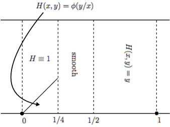
Figure 1. Illustration of the function $H(x,y)$ from [5] used in the proof of the upper bound for Theorem 4.2.

Since the finite Zak transform is unitary, it follows that there exists a sequence $b\in\ell^{d}_{2}$ of unit norm so that

$$Z_{d}(b)(m,n)=G\Big{(}\frac{m}{N},\frac{n}{N}\Big{)}.$$ (35)

In particular, since $G$ is unimodular, it follows by Proposition 2.7 that the Gabor system $G_{d}(b)$ is an orthonormal basis for $\ell_{2}^{d}$.

The following proposition provides the required estimate from above on $\beta_{1,1}(N)$.

Proposition 4.5.

Let $b$ be the sequence defined above. Then, there exists a constant $C>0$ so that for all $N\geq 2$ and $d=N^{2}$, we have

$$\beta(b,N)\leq C\log N.$$ (36)

Proof.

In this proof, we denote by $C$ positive constants which may change from line to line. In light of (35), we need to estimate the expression

$$\underbrace{\sum_{m,n=0}^{N-1}\Big{|}\Delta G\Big{(}\frac{m}{N},\frac{n}{N}\Big{)}\Big{|}^{2}}_{:=(I)}+\underbrace{\sum_{m,n=0}^{N-1}\Big{|}\Gamma G\Big{(}\frac{m}{N},\frac{n}{N}\Big{)}\Big{|}^{2}}_{:=(II)}.$$

To estimate $(I)$, we make the following partition of the set $[0,N-1]^{2}\cap\mathbb{Z}^{2}$:

$$A_{0} =\{(m,n)\in\mathbb{Z}^{2}:m\in[0,N/8],n=0\}$$

$$A_{1} =\{(m,n)\in\mathbb{Z}^{2}:m\in[1,N/8]\text{ and }n\in[1,m]\}$$

$$A_{2} =([0,N-1]^{2}\cap\mathbb{Z}^{2})\backslash(A_{0}\cup A_{1})$$

On $A_{0}$, the values of $G(m/N,n/N)$ are constant, so

$$\sum_{(m,n)\in A_{0}}\Big{|}\Delta G\Big{(}\frac{m}{N},\frac{n}{N}\Big{)}\Big{|}^{2}=0.$$

On $A_{2}$, we use the fact that the function $G$ is $C^{\infty}$ on $\mathbb{R}^{2}\backslash\mathbb{Z}^{2}$, and moreover, that on the set $\{(x,y)\in[0,1]^{2}:y\geq x\vee x\geq 1/8\}$ both $G$, and its derivatives, are continuous. Indeed, this means that we are justified in using the Mean Value theorem for $(m,n)\in A_{2}$ to make the estimate

$$\Big{|}\Delta G\Big{(}\frac{m}{N},\frac{n}{N}\Big{)}\Big{|} =\frac{1}{N}\cdot\Big{|}(\partial_{x}G)\Big{(}\mu_{m,n},\frac{n}{N}\Big{)}\Big{|}\leq\frac{C}{N},$$

where $\mu_{m,n}\in(m/N,(m+1)/N)$ and $C=C(G)>0$ is a constant not depending on $N$. It follows immediately that

$$\sum_{(m,n)\in A_{2}}\Big{|}\Delta G\Big{(}\frac{m}{N},\frac{n}{N}\Big{)}\Big{|}^{2}\leq\frac{1}{N^{2}}\cdot C|A_{2}|\leq C.$$

On $A_{1}$, we do the computation

$$\sum_{(m,n)\in A_{1}}\Big{|}\Delta G\Big{(}\frac{m}{N},\frac{n}{N}\Big{)}\Big{|}^{2}=\underbrace{\sum_{m=1}^{[N/8]}\,\,\sum_{n=1}^{m}\Big{|}(\partial_{x}G\Big{(}\mu_{m,n},\frac{n}{N}\Big{)}\Big{|}^{2}\frac{1}{N^{2}}}_{:=\,(*)},$$

where $\mu_{m,n}\in(m/N,(m+1)/N)$ as before. To estimate $(*)$, we compute

$$\Big{|}(\partial_{x}G)\Big{(}x,\frac{n}{N}\Big{)}\Big{|} =2\pi\Big{|}(\partial_{x}H)\Big{(}x,\frac{n}{N}\Big{)}\Big{|}$$

$$=2\pi\Big{|}\partial_{x}\phi\Big{(}\frac{n}{Nx}\Big{)}\Big{|}$$

$$=2\pi\Big{|}\phi^{\prime}\Big{(}\frac{n}{Nx}\Big{)}\Big{|}\cdot\frac{n}{Nx^{2}}.$$

This allows the bound

$$(\ast) =4\pi^{2}\sum_{m=1}^{[N/8]}\sum_{n=1}^{m}\Big{|}\phi^{\prime}\Big{(}\frac{n}{N\mu_{m,n}}\Big{)}\Big{|}^{2}\frac{n^{2}}{N^{4}\mu_{m,n}^{4}}$$

$$\leq\frac{4\pi^{2}\|\phi^{\prime}\|_{\infty}^{2}}{N^{4}}\sum_{m=1}^{[N/8]}\sum_{n=1}^{m}\frac{n^{2}}{(m/N)^{4}}$$

$$\leq 4\pi^{2}\|\phi^{\prime}\|_{\infty}^{2}\sum_{m=1}^{[N/8]}\frac{1}{m^{4}}\cdot(m+1)^{3}$$

$$\leq 4\pi^{2}\|\phi^{\prime}\|_{\infty}^{2}\Big{(}C+\log N\Big{)}.$$

To estimate (II), we consider the corresponding sums over $A_{2}$ and over $B=A_{0}\cup A_{1}$. We skip the estimates for $A_{2}$, which are completely analogous to the corresponding estimates made above. Instead, we turn our focus to the estimate for $B$. As above, we begin by using the Mean Value Theorem to write

$$\sum_{(m,n)\in B}\Big{|}\Gamma G\Big{(}\frac{m}{N},\frac{n}{N}\Big{)}\Big{|}^{2}=\underbrace{\sum_{m=1}^{[N/8]}\,\,\sum_{n=0}^{m}|(\partial_{y}G)\Big{(}\frac{m}{N},\nu_{m,n}\Big{)}|^{2}\frac{1}{N^{2}}}_{:=\,(**)},$$

where $\nu_{m,n}\in[n/N,(n+1)/N]$. To estimate $(**)$, we compute

$$\Big{|}(\partial_{y}G)\Big{(}\frac{m}{N},y\Big{)}\Big{|} =2\pi\Big{|}(\partial_{y}H)\Big{(}\frac{m}{N},y\Big{)}\Big{|}$$

$$=2\pi\Big{|}\partial_{y}\phi\Big{(}\frac{Ny}{m}\Big{)}\Big{|}$$

$$=2\pi\Big{|}\phi^{\prime}\Big{(}\frac{Ny}{m}\Big{)}\Big{|}\cdot\frac{N}{m}.$$

This allows the estimate

$$(**) =4\pi^{2}\sum_{m=1}^{[N/8]}\,\,\sum_{n=0}^{m}\Big{|}\phi^{\prime}\Big{(}\frac{N\nu_{m,n}}{m}\Big{)}\Big{|}^{2}\cdot\frac{1}{N^{2}}\cdot\frac{N^{2}}{m^{2}}$$

$$\leq 4\pi^{2}\|\phi^{\prime}\|^{2}_{\infty}\sum_{m=1}^{[N/8]}\,\,\sum_{n=0}^{m}\frac{1}{m^{2}}$$

$$\leq 4\pi^{2}\|\phi^{\prime}\|^{2}_{\infty}\sum_{m=1}^{[N/8]}\frac{m+1}{m^{2}}$$

$$\leq 4\pi^{2}\|\phi^{\prime}\|^{2}_{\infty}\Big{(}C+\log N\Big{)}.$$

∎

Remark 4.6.

To determine a bound for the constant $C$ of inequality (36), observe that we can actually choose $\phi$ to be piecewise linear, and therefore to satisfy $\|\phi^{\prime}\|_{\infty}^{2}\leq 1$. Moreover, observe that

$$(*)+(**)\leq 8\pi^{2}(C_{0}+\log N),$$

where $C_{0}$ is some positive constant. Since the remaining sums over $A_{2}$ only contribute to $C_{0}$, we conclude that asymptotically,

$$C\leq\lim_{N_{0}\rightarrow\infty}\Big{(}\sup_{N\geq N_{0}}\frac{\beta_{1,1}(N)}{\log N}\Big{)}\leq 8\pi^{2}.$$

5. A quantitative Balian-Low type theorem in finite dimensions

In this section, we prove a finite dimensional version of the quantitative Balian-Low inequality. For the most part, we follow the main ideas appearing in our paper [24].

5.1. Auxiliary results

The estimate in the following lemma is not optimal, but rather, chosen to simplify the presentation.

Lemma 5.1.

Let $\rho:\mathbb{R}\rightarrow\mathbb{R}$ be the inverse Fourier transform of

$$\hat{\rho}(\xi)=\left\{\begin{aligned} 1&\qquad|\xi|\leq 1/2,\\[5.69054pt] 2(1-\xi\operatorname{sgn}(\xi))&\qquad 1/2\leq|\xi|\leq 1,\\[5.69054pt] 0&\qquad|\xi|\geq 1.\end{aligned}\right.$$

Then

$$\int_{\mathbb{R}}|\rho^{\prime}(t)|\mathrm{d}t\leq 10.$$

Proof.

Fix $b>0$ to be chosen later. We make the split

$$\int_{\mathbb{R}}|\rho^{\prime}(t)|\mathrm{d}t=\underbrace{\int_{-b}^{b}|\rho^{\prime}(t)|\mathrm{d}t}_{=(I)}+\underbrace{\int_{|t|\geq b}|\rho^{\prime}(t)|\mathrm{d}t}_{=(II)}.$$

To estimate (I), we compute

$$|\rho^{\prime}(t)| =|\mathcal{F}^{-1}\Big{(}2\pi\mathrm{i}\xi\cdot\hat{\rho}\Big{)}(t)|$$

$$\leq 2\pi\|\xi\cdot\hat{\rho}\|_{L^{1}(\mathbb{R})}={2\pi}\cdot\frac{7}{12}=\frac{7\pi}{6},$$

whence

$$(I)\leq\frac{7\pi}{6}\cdot 2b=\frac{7\pi b}{3}.$$

We turn to estimate (II). Integrating by parts, we find that

$$\rho^{\prime}(t)=\mathcal{F}^{-1}\Big{(}2\pi\mathrm{i}\xi\cdot\hat{\rho}\Big{)}(t) =2\pi\mathrm{i}\int_{\mathbb{R}}\xi\hat{\rho}(\xi)\cdot\mathrm{e}^{2\pi\mathrm{i}\xi t}\,\mathrm{d}\xi$$

$$=-2\pi\mathrm{i}\int_{\mathbb{R}}(\hat{\rho}+\xi\hat{\rho}^{\prime})\cdot\frac{\mathrm{e}^{2\pi\mathrm{i}\xi t}}{2\pi\mathrm{i}t}\,\mathrm{d}\xi$$

$$=2\pi\mathrm{i}\int_{\mathbb{R}}(2\hat{\rho}^{\prime}+\xi\hat{\rho}^{\prime\prime})\frac{\mathrm{e}^{2\pi\mathrm{i}\xi t}}{(2\pi\mathrm{i}t)^{2}}\,\mathrm{d}\xi$$

$$=\frac{1}{\pi\mathrm{i}t^{2}}\int_{\mathbb{R}}\hat{\rho}^{\prime}(\xi)\mathrm{e}^{2\pi\mathrm{i}\xi t}\mathrm{d}\xi+\frac{1}{\pi t^{2}}\Big{(}2\sin(2\pi t)-\sin(\pi t)\Big{)}.$$

This yields the bound

$$|\rho^{\prime}(t)|\leq\frac{1}{\pi t^{2}}\Big{(}\int_{\mathbb{R}}|\hat{\rho}^{\prime}|\mathrm{d}\xi+2+1\Big{)}=\frac{5}{\pi t^{2}},$$ (37)

and the estimate

$$(II)\leq\frac{10}{\pi}\int_{b}^{\infty}\frac{dt}{t^{2}}=\frac{10}{\pi b}.$$

We compute the value of $b$ which minimizes the bound we obtained for (I)+(II) and find that this value is $b=\sqrt{30/7}/\pi$, which gives us the estimate $(I)+(II)\leq 9.67<10$.

∎

Lemma 5.2.

Let $A,B>0$ and $N\geq 200\sqrt{B/A}$. There exist positive constants $\delta=\delta(A)$ and $C=C(A,B)$ such that the following holds (with $d=N^{2}$). Let

• $Q,R\in\mathbb{Z}$ such that $1\leq Q,R\leq(N/16)\cdot\sqrt{A/B}$,

• $\phi,\psi\in\ell_{2}^{d}$ such that $\sum_{n}|\Delta\phi(n)|\leq 10R$ and $\sum_{n}|\Delta\psi(n)|\leq 10Q$,

• $b\in\ell_{2}^{d}$ such that $A\leq|Z_{d}(b)|^{2}\leq B$.

Then, there exists a set $S\subset([0,N-1]\cap\mathbb{Z})^{2}$ of size $|S|\geq CN^{2}/QR$ such that all $(u,v)\in S$ satisfy either

$$|Z_{d}(b)(u,v)-Z_{d}(b\ast\phi)(u,v)|\geq\delta,\qquad\text{or}$$ (38)

$$|Z_{d}(\mathcal{F}_{d}b)(u,v)-Z_{d}((\mathcal{F}_{d}b)\ast\psi)(u,v)|\geq\delta.$$ (39)

Proof of Lemma 5.2.

For the given $A$ and for $N_{0}=200$, let $\delta_{1}=2\sqrt{A}\sin(\pi/4-\pi/{200})$ be the constant from Corollary 3.6. Notice that the integers $Q,R$ and $N$ satisfy

$$\frac{\sqrt{B}}{\delta_{1}}\max\Big{\{}{\frac{200R}{9}},{\frac{200Q}{9}},{80\pi}\Big{\}}{\leq}N.$$

Therefore, there exist integers $K$ and $L$ that satisfy

$${\frac{200\sqrt{B}R}{9\delta_{1}}}{\leq}K\leq N\qquad\text{and}\qquad\frac{\sqrt{B}}{\delta_{1}}\max\Big{\{}{\frac{200Q}{9},80\pi}\Big{\}}{\leq}L\leq N.$$ (40)

We choose $K,L$ to be the smallest such integers.

For $s,t\in\mathbb{Z}$, let $\sigma_{s}$ and $\omega_{t}$ be as defined in (23), that is,

$$\sigma_{s}=\Big{[}\frac{sN}{K}\Big{]},\qquad\textrm{and}\qquad\omega_{t}=\Big{[}\frac{tN}{L}\Big{]}.$$

Note that $\sigma_{K}=\omega_{L}=N$ and denote $\Sigma=\inf\{\Delta_{(s)}\sigma_{s}\}$ and $\Omega=\inf\{\Delta_{(t)}\omega_{t}\}$. The conditions on $K$ and $L$ imply that, for some constant $C_{1}=C_{1}(A,B)$,

$$\Sigma\cdot\Omega\geq C_{1}\frac{N^{2}}{QR}.$$

For $(u,v)\in([0,\Sigma-1]\cap\mathbb{Z})\times([0,\Omega-1]\cap\mathbb{Z})$, write

$$\mathrm{Lat}(u,v)=\big{\{}(u+\sigma_{s},v+\omega_{t}):(s,t)\in([0,K-1]\cap\mathbb{Z})\times([0,L-1]\cap\mathbb{Z})\big{\}}.$$

and

$$\mathrm{Lat^{*}}(u,v)=\big{\{}(N-v-\omega_{t},u+\sigma_{s}):(s,t)\in([0,K-1]\cap\mathbb{Z})\times([0,L-1]\cap\mathbb{Z})\big{\}}.$$

Note that if $(u_{1},v_{1})\neq(u_{2},v_{2})$ then it follows from the definition of $\Sigma$ and $\Omega$ that $\mathrm{Lat}(u_{1},v_{1})\cap\mathrm{Lat}(u_{2},v_{2})=\emptyset$ and $\mathrm{Lat^{*}}(u_{1},v_{1})\cap\mathrm{Lat^{*}}(u_{2},v_{2})=\emptyset$. We will show that for each $(u,v)$, either the set $\mathrm{Lat}(u,v)$ or the set $\mathrm{Lat^{*}}(u,v)$ contains a point from $([0,N-1]\cap\mathbb{Z})^{2}$ which satisfies condition (38) or (39), respectively. Putting $C=C_{1}/2$ our proof will then be complete.

So, fix $(u,v)\in([0,\Sigma-1]\cap\mathbb{Z})\times([0,\Omega-1]\cap\mathbb{Z})$. Due to Corollary 3.6, there exists at least one point $(s,t)\in([0,K-1]\cap\mathbb{Z})\times([0,L-1]\cap\mathbb{Z})$ such that (26) or (27) hold with $W=Z_{d}(b)$.

Assume first that (26) holds. Lemma 2.6, the estimate $|\Delta_{(s)}\sigma_{s}|\leq 2N/K$, and condition (40), imply that

$$|\Delta_{(s)}Z_{d}(b\ast\phi)(u+\sigma_{s},v+\omega_{t})|\leq\frac{2N/K}{N}\cdot\sqrt{B}\cdot{10}R\leq\frac{9\delta_{1}}{10}.$$

It follows that either $(u+\sigma_{s},v+\omega_{t})$ or $(u+\sigma_{(s+1)},v+\omega_{t})$ satisfy (38) with $\delta=\delta_{1}/20$. It may happen that this chosen point does not belong to $([0,N-1]\cap\mathbb{Z})^{2}$, that is, it is of the form $(u+N,v+\omega_{t})$. In that case, due to the $N$-quasi-periodicity of the Zak transform, the point $(u,v+\omega_{t})$ satisfies the same inequality, and is in $([0,N-1]\cap\mathbb{Z})^{2}$.

Assume now that (27) holds for $(u,v)$ and $(s,t)$. Then (13), the $N$-quasi-periodicity of $Z_{d}(b)$, and the estimate $|\Delta_{(t)}\omega_{t}|\leq{2N/L}$, imply that

$$|\Delta_{(t)}Z_{d}(\mathcal{F}_{d}b)(N-v-\omega_{t},u+\sigma_{s})|$$

$$=\Big{|}Z_{d}(b)(u+\sigma_{s},v+\omega_{t+1})-e^{2\pi i\frac{(\omega_{t+1}-\omega_{t})(u+\sigma_{s})}{d}}Z_{d}(b)(u+\sigma_{s},v+\omega_{t})\Big{|}$$

$$\geq|\Gamma_{(t)}Z_{d}(b)(u+\sigma_{s},v+\omega_{t})|-\sqrt{B}|e^{2\pi i\frac{(\omega_{t+1}-\omega_{t})(u+\sigma_{s})}{d}}-1|$$

$$\geq\delta_{1}-{\frac{4\pi\sqrt{B}}{L}}\geq\frac{19\delta_{1}}{20}.$$

On the other hand, as in the previous case, we have

$$|\Delta_{(t)}Z_{d}(\mathcal{F}_{d}b\ast\psi)(N-v-\omega_{t},u+\sigma_{s})|\leq\frac{{20}\sqrt{B}Q}{L}<\frac{9\delta_{1}}{10}.$$

It follows that either $(N-v-\omega_{t},u+\sigma_{s})$ or $(N-v-\omega_{(t+1)},u+\sigma_{s})$ satisfy (39) with $\delta=\delta_{1}/40$. It may happen that this chosen point is the point $(-v,u+\sigma_{s})$. In that case, due to the $N$-quasi-periodicity of the Zak transform, the point $(N-v,u+\sigma_{s})$ satisfies the same inequality, and is in $([0,N-1]\cap\mathbb{Z})^{2}$. ∎

5.2. A proof for Theorem 1.5

We are now ready to prove Theorem 1.5. In fact, we prove the more general version referred to in Remark 1.6 which we formulate as follows:

Theorem 5.3.

Let $A,B>0$. There exists a constant $C=C(A,B)>0$ so that the following holds. Let $N\geq 200\sqrt{B/A}$ and let $b\in\ell_{2}^{d}$ (where $d=N^{2}$) be such that $G_{d}(b)$ is a basis in $\ell_{2}^{d}$ with Riesz basis bounds $A$ and $B$. Then, for all positive integers $1\leq Q,R\leq(N/{16})\cdot\sqrt{A/B}$, we have

$$\frac{1}{N}\sum_{j=NQ}^{d-1}|b(j)|^{2}+\frac{1}{N}\sum_{k=NR}^{d-1}|\mathcal{F}_{d}b(k)|^{2}\geq\frac{C}{QR}.$$

Proof of Theorem 1.5.

Let $\rho:\mathbb{R}\rightarrow{\mathbb{R}}$ be as in Lemma 5.1 and put $\Phi(t)=R\rho(Rt)$ and $\Psi(t)=Q\rho(Qt)$. Denote $\phi=S_{N}P_{N}\Phi$ and $\psi=S_{N}P_{N}\Psi$. By Lemma 2.10, in combination with Lemma 5.1, it follows that $\sum_{n}|\Delta\phi(n)|\leq{10}R$ and $\sum_{n}|\Delta\psi(n)|\leq{10}Q$. As a consequence, the integers $Q,R$ and $N$, as well as the functions $\phi,\psi$ and $b$, all satisfy the requirements of Lemma 5.2.

As $Q,R<N/2$, by Proposition 2.8, and Remark 2.9(i), we have $0\leq\mathcal{F}_{d}\phi,\mathcal{F}_{d}\psi\leq 1$ over $\ell_{2}^{d}$. Moreover, we also have $\mathcal{F}_{d}\phi(j)=1$ for $j\in[0,RN/2]\cup[N^{2}-RN/2+1,N^{2}]$ and $\mathcal{F}_{d}\psi(j)=1$ for $j\in[0,QN/2]\cup[N^{2}-QN/2+1,N^{2}]$. It therefore follows from Lemma 5.2, and the fact that both the finite Zak transform and the finite Fourier transform are unitary, that, for some constant $C>0$,

$$\frac{C}{QR} \leq\|Z_{d}(b)-Z_{d}(b\ast\phi)\|_{\ell_{2}([0,N-1]^{2})}^{2}$$

$$\hskip 85.35826pt+\|Z_{d}(\mathcal{F}_{d}b)-Z_{d}(\mathcal{F}_{d}b\ast\psi)\|_{\ell_{2}([0,N-1]^{2})}^{2}$$

$$=\|b-b\ast\phi\|_{\ell^{2}_{d}}^{2}+\|\mathcal{F}_{d}b-\mathcal{F}_{d}b\ast\psi\|_{\ell^{2}_{d}}^{2}$$

$$=\|\mathcal{F}_{d}b(1-\mathcal{F}_{d}\phi)\|_{\ell^{2}_{d}}^{2}+\|b(1-\mathcal{F}_{d}\psi)\|_{\ell^{2}_{d}}^{2}$$

$$\leq\frac{1}{N}\sum_{k=[NR/2]+1}^{d-1-[NR/2]}|\mathcal{F}_{d}b(k)|^{2}+\frac{1}{N}\sum_{j=[NQ/2]+1}^{d-1-[NQ/2]}|b(j)|^{2}.$$

The result now follows by applying a suitable time-frequency translate to the sequence $b$. ∎

6. Applications to the continuous setting

In this section we show that both the classical and quantitative Balian-Low theorems follow from their finite dimensional analogs.

6.1. Relating continuous and finite signals – revisited

We start by extending Proposition 2.8 to the space $L^{2}(\mathbb{R})$. We do this in four steps. In the first, we introduce some additional notations. To this end, fix $N\in\mathbb{N}$, $N\geq 2$, and let $d=N^{2}$.

Step I: By $(L^{2}[0,1/N]^{2})^{d}$, we denote the space of all d-tuples $\{\phi(j)\}_{j=0}^{d-1}$ with function entries $\phi(j)\in L^{2}([0,{1}/{N}]^{2})$, equipped with the norm given by

$$\|\{\phi(j)\}\|_{(L^{2}[0,1/N]^{2})^{d}}^{2}=N\sum_{j=0}^{d-1}\|\phi(j)\|^{2}_{L^{2}([0,1/N]^{2})}.$$

Note that the factor $N$ appears in the norm in order to take the measure of $[0,{1}/{N}]$ into account. Similarly, by $(L^{2}[0,1/N]^{2})^{N\times N}$, we denote the space of all $N\times N$ matrices $\{\phi(j,k)\}_{j,k=0}^{N-1}$ with function entries $\phi(j,k)\in L^{2}([0,{1}/{N}]^{2})$, equipped with norm given by

$$\|\{\phi(j,k)\}\|_{(L^{2}[0,1/N]^{2})^{N\times N}}^{2}=\sum_{j,k=0}^{N-1}\|\phi(j,k)\|^{2}_{L^{2}([0,1/N]^{2})}.$$

Step II: We consider functions $h(u,v;t)$ defined over $[0,{1}/{N}]^{2}\times\mathbb{R}$, that are $N$-periodic with respect to the variable $t$, and are such that, for every fixed $t_{0}$, the restriction $h(u,v;t_{0})$ is well defined almost everywhere and belongs to $L^{2}([0,1/N]^{2})$. Observe that the operator

$$S_{N}\,h:=\{h(u,v;j/N)\}_{j=0}^{d-1}$$

trivially satisfies

$$S_{N}h\in(L^{2}[0,{1}/{N}]^{2})^{d},$$ (41)

$$\mathcal{F}_{d}S_{N}h\in(L^{2}[0,{1}/{N}]^{2})^{d},$$ (42)

$$Z_{d}S_{N}h\in(L^{2}[0,{1}/{N}]^{2})^{N\times N}.$$ (43)

Above, we understand the notations $\mathcal{F}_{d}S_{N}h$ and $Z_{d}S_{N}h$ to mean that $\mathcal{F}_{d}$ and $Z_{d}$ operate on $S_{N}h$ with respect to the variable $j$ with $(u,v)$ being considered fixed.

Step III: Let $f\in L^{2}(\mathbb{R})$. For $(u,v)\in[0,{1}/{N}]^{2}$, we define the function

$$f_{(u,v)}(t):=\mathrm{e}^{2\pi\mathrm{i}vt}f(t+u),\qquad t\in\mathbb{R}$$

and formally put

$$P_{N}{f}_{(u,v)}(t):=\sum_{\ell=-\infty}^{\infty}f_{(u,v)}(t+\ell N).$$

Note that if $f$ is in the Schwarz class $\mathcal{S}(\mathbb{R})$, then the function $h(u,v;t):=P_{N}{f}_{(u,v)}(t)$ satisfies the conditions on $h(u,v;t)$ described in Step II. The following lemma shows that this is true for all $f\in L^{2}(\mathbb{R})$.

Lemma 6.1.

For $f\in L^{2}(\mathbb{R})$, let $f_{(u,v)}(t)$ be the function defined above. Then, for every fixed $t_{0}\in\mathbb{R}$, we have

$$P_{N}{f}_{(u,v)}(t_{0})\in L^{2}([0,1/N]^{2}).$$

That is, the series defining $P_{N}f_{(u,v)}(t_{0})$ converges in the norm of $L^{2}([0,1/N]^{2})$.

Proof.

The lemma follows from the following computation, where, in the first step, we use the fact that $\{\sqrt{N}\mathrm{e}^{2\pi\mathrm{i}N\ell v}\}_{\ell\in\mathbb{Z}}$ is an orthonormal basis over $[0,1/N]$:

$$\int_{0}^{\frac{1}{N}}\int_{0}^{\frac{1}{N}}\Big{|}\sum_{|\ell|>L}f(t_{0}+u+\ell N) \mathrm{e}^{2\pi\mathrm{i}N\ell v}\Big{|}^{2}\mathrm{d}v\mathrm{d}u$$

$$=\frac{1}{N}\sum_{|\ell|>L}\int_{0}^{\frac{1}{N}}|f(t_{0}+u+\ell N)|^{2}\mathrm{d}u$$

$$\leq\frac{1}{N}\int_{|x-t_{0}|\geq L/2}|f(x)|^{2}\mathrm{d}x\rightarrow 0,\quad\text{as }L\rightarrow\infty.$$

∎

It follows that, for $f\in L^{2}(\mathbb{R})$, the operator $S_{N}P_{N}f_{(u,v)}$ is well defined and that conditions (41), (42), (43) hold with $h(u,v;t)=P_{N}f_{(u,v)}(t)$.

Step IV: For $f$ in $L^{2}(\mathbb{R})$, we understand the notations $\mathcal{F}f_{(u,v)}(t)$ and $Zf_{(u,v)}(t)$ to mean that the Fourier transform and the Zak transform are taken with respect to the variable $t$, with $(u,v)$ being fixed. We now give our extension of Proposition 2.8.

Proposition 6.2.

Let $f\in L^{2}(\mathbb{R})$. Then, the following hold.

• For all $N\in\mathbb{N}$ and $(m,n)\in\mathbb{Z}^{2}$, we have

  $$Z_{d}(S_{N}{P_{N}f_{(u,v)}})(m,n)=Zf_{(u,v)}(m/N,n/N),$$ (44)

  where the equality holds in the sense of ${L^{2}([0,{1}/{N}]^{2})}$.

• For all $N\in\mathbb{N}$, we have

  $$\mathcal{F}_{d}S_{N}P_{N}{f_{(u,v)}}=S_{N}P_{N}\mathcal{F}f_{(u,v)},$$ (45)

  where the equality holds in the sense of $(L^{2}[0,{1}/{N}]^{2})^{d}$.

Proof.

First, Proposition 2.8 implies that (44) and (45) hold for $f\in\mathcal{S}(\mathbb{R})$ pointwise everywhere. Since $\mathcal{S}(\mathbb{R})$ is dense in $L^{2}(\mathbb{R})$, it is enough to show that the four operators implicitly defined by the left and right-hand sides of (44) and (45) are isometric (in fact, they are unitary).

To establish (45), we start by noting that $T_{1}:\mathcal{S}(\mathbb{R})\rightarrow(L^{2}[0,{1}/{N}]^{2})^{d}$, defined by $(T_{1}f)(u,v)=S_{N}{P_{N}f_{(u,v)}},$ is isometric. Indeed,

$$\|S_{N}{P_{N}f_{(u,v)}}\|^{2}_{(L^{2}[0,{1}/{N}]^{2})^{d}} =N\sum_{j=0}^{N^{2}-1}\iint_{[0,\frac{1}{N}]^{2}}\ \Big{|}\sum_{\ell=-\infty}^{\infty}f\Big{(}\frac{j}{N}+u+\ell N\Big{)}\mathrm{e}^{2\pi\mathrm{i}vlN}\Big{|}^{2}\,\mathrm{d}v\mathrm{d}u$$

$$=\sum_{\ell=-\infty}^{\infty}\sum_{j=0}^{N^{2}-1}\int_{0}^{\frac{1}{N}}\Big{|}f\Big{(}\frac{j}{N}+u+\ell N\Big{)}\Big{|}^{2}\,\mathrm{d}u=\|f\|^{2}_{L^{2}(\mathbb{R})}.$$

Since the finite Fourier transform $\mathcal{F}_{d}$ is unitary, we conclude that $\mathcal{F}_{d}\circ T_{1}$, implicitly defined on the left hand side of (45), is also unitary. Next, we note that $\mathcal{F}(f_{(u,v)})=e^{-2\pi iuv}(\mathcal{F}f)_{(-v,u)}$. Since both the Fourier transform $\mathcal{F}$ and the operator $T_{1}$ are unitary, we conclude that the operator implicitly defined on the right hand side of (45) is also unitary, and therefore that (45) holds for all $f\in L^{2}(\mathbb{R})$.

To obtain (44) we first note that, since the discrete Zak transform is unitary, the above computation also implies that the operator defined by the left-hand side of (45), which acts from $L^{2}(\mathbb{R})$ to $(L^{2}[0,{1}/{N}]^{2})^{N\times N}$, is isometric. To complete the proof of Proposition 6.2, it therefore remains to show that the same is true for the operator $T_{2}:\mathcal{S}(\mathbb{R})\mapsto(L^{2}[0,{1}/{N}]^{2})^{N\times N}$, defined by $(T_{2}f)(u,v)=\{Zf_{(u,v)}({m}/{N},{n}/{N})\}_{m,n=0}^{N-1}.$ To see this, we let $f\in\mathcal{S}(\mathbb{R})$, and make the following computation:

$$\Big{\|}\Big{\{}Zf_{(u,v)} \Big{(}\frac{m}{N},\frac{n}{N}\Big{)}\Big{\}}\Big{\|}^{2}_{(L^{2}[0,{1}/{N}]^{2})^{N\times N}}=$$

$$=\sum_{m,n=0}^{N-1}\iint_{[0,\frac{1}{N}]^{2}}\Big{|}\sum_{\ell=-\infty}^{\infty}f\Big{(}\frac{m}{N}+u-\ell\Big{)}e^{-2\pi iv\ell}e^{2\pi i\frac{n\ell}{N}}\Big{|}^{2}\mathrm{d}v\mathrm{d}u$$

$$=\sum_{m=0}^{N-1}\int_{[0,\frac{1}{N}]}\int_{[0,1]}\Big{|}\sum_{\ell=-\infty}^{\infty}f\Big{(}\frac{m}{N}+u-\ell\Big{)}e^{-2\pi iv\ell}\Big{|}^{2}\mathrm{d}v\mathrm{d}u$$

$$=\sum_{m=0}^{N-1}\int_{[0,\frac{1}{N}]}\sum_{\ell=-\infty}^{\infty}\Big{|}f\Big{(}\frac{m}{N}+u-\ell\Big{)}\Big{|}^{2}\mathrm{d}u=\|f\|^{2}_{L^{2}(\mathbb{R})}.$$

∎

In particular, we have the following.

Corollary 6.3.

Let $g\in L^{2}(\mathbb{R})$ be such that the Gabor system $G(g)$ is a Riesz basis in $L^{2}(\mathbb{R})$ with lower and upper Riesz basis bounds $A$ and $B$, respectively. Then, for almost every $(u,v)\in[0,{1}/{N}]^{2}$, the Gabor system $G_{d}(S_{N}P_{N}g_{(u,v)})$ is a Riesz basis in $\ell_{2}^{d}$ with lower and upper Riesz basis bounds $\widetilde{A}$ and $\widetilde{B}$ satisfying $A\leq\widetilde{A}$ and $\widetilde{B}\leq B$, respectively.

Proof.

In light of Proposition 2.7, this result follows immediately from part (i) of Proposition 6.2. ∎

6.2. The classical Balian-Low theorem

We start with the following lemma which relates the discrete and continuous derivatives of $L^{2}(\mathbb{R})$ functions.

Lemma 6.4.

Let $f\in L^{2}(\mathbb{R})$ and $N\in\mathbb{N}$. Denote $F_{(u,v)}=S_{N}P_{N}f_{(u,v)}$. Then,

$$N^{2}\|\Delta_{(j)}F_{(u,v)}(j)\|_{(L^{2}[0,{1}/{N}]^{2})^{d}}^{2}\leq 2\int_{\mathbb{R}}|f^{\prime}(t)|^{2}\mathrm{d}t+\frac{8\pi^{2}}{N^{2}}\int_{\mathbb{R}}|f(t)|^{2}\mathrm{d}t,$$

where the integral on the right-hand side is understood to be infinite if $f$ is not absolutely continuous, or if its derivative is not in $L^{2}(\mathbb{R})$.

Proof.

Put $a_{u}(j,l)=f(u+\frac{j}{N}+\ell N)$ and fix $j\in[0,N^{2}-1]\cap\mathbb{Z}$. Since $f\in L^{2}(\mathbb{R})$, we have, with respect to the variable $\ell$, that $a_{u}(j,\ell)\in\ell_{2}(\mathbb{Z})$ for almost every $u$. We compute

$$\iint_{[0,\frac{1}{N}]^{2}} |\Delta_{(j)}F_{(u,v)}(j)|^{2}\,\mathrm{d}v\mathrm{d}u=$$

$$=\iint_{[0,\frac{1}{N}]^{2}}\Big{|}\sum_{\ell=-\infty}^{\infty}\Big{(}a_{u}(j+1,l)\,\mathrm{e}^{2\pi i\frac{v(j+1)}{N}}-a_{u}(j,l)\,\mathrm{e}^{2\pi i\frac{vj}{N}}\Big{)}\,\mathrm{e}^{2\pi\mathrm{i}vlN}\Big{|}^{2}\,\mathrm{d}v\mathrm{d}u$$

$$\leq 2\iint_{[0,\frac{1}{N}]^{2}}\Big{|}\sum_{\ell=-\infty}^{\infty}\Delta_{(j)}a_{u}(j,l)\,\mathrm{e}^{2\pi\mathrm{i}vN\ell}\Big{|}^{2}\mathrm{d}u\mathrm{d}v$$

$$\hskip 85.35826pt+2\iint_{[0,\frac{1}{N}]^{2}}\Big{|}\Big{(}\mathrm{e}^{2\pi i\frac{{v}}{N}}-1\Big{)}\sum_{\ell=-\infty}^{\infty}a_{u}(j,l)\,\mathrm{e}^{2\pi\mathrm{i}vlN}\Big{|}^{2}\,\mathrm{d}v\mathrm{d}u$$

$$\leq\frac{2}{N}\sum_{\ell=-\infty}^{\infty}\int_{0}^{\frac{1}{N}}|a_{u}(j+1,l)-a_{u}(j,l)|^{2}\,\mathrm{d}u+\frac{8\pi^{2}}{N^{5}}\sum_{\ell=-\infty}^{\infty}\int_{0}^{\frac{1}{N}}|a_{u}(j,l)|^{2}\,\mathrm{d}u,$$

where we applied the inequality $|a+b|^{2}\leq 2|a|^{2}+2|b|^{2}$ in the second step and the inequality $|e^{ix}-1|\leq|x|$ in the third step. By the Cauchy-Schwartz inequality, we get

$$\int_{0}^{\frac{1}{N}}\Big{|}a_{u}(j+1,l)-a_{u}(j,l)\Big{|}^{2}\,\mathrm{d}u =\int_{0}^{\frac{1}{N}}\Big{|}\int_{\frac{j}{N}+\ell N}^{\frac{j+1}{N}+\ell N}f^{\prime}(t+u)\mathrm{d}t\Big{|}^{2}\,\mathrm{d}u$$

$$\leq\frac{1}{N}\int_{0}^{\frac{1}{N}}\int_{\frac{j}{N}+\ell N}^{\frac{j+1}{N}+\ell N}|f^{\prime}(t+u)|^{2}\,\mathrm{d}t\mathrm{d}u.$$

Combining these two estimates we find that

$$N^{2}\| \Delta F_{(u,v)}(j)\|_{(L^{2}[0,{1}/{N}]^{2})^{d}}^{2}=N^{3}\sum_{j=0}^{N^{2}-1}\iint_{[0,\frac{1}{N}]^{2}}|\Delta F_{(u,v)}(j)|^{2}\,\mathrm{d}v\mathrm{d}u$$

$$\leq 2N\sum_{\ell=-\infty}^{\infty}\sum_{j=0}^{N^{2}-1}\int_{0}^{\frac{1}{N}}\int_{\frac{j}{N}+\ell N}^{\frac{j+1}{N}+\ell N}|f^{\prime}(t+u)|^{2}\,\mathrm{d}t\mathrm{d}u$$

$$\hskip 170.71652pt+\frac{8\pi^{2}}{N^{2}}\sum_{\ell=-\infty}^{\infty}\sum_{j=0}^{N^{2}-1}\int_{0}^{\frac{1}{N}}|\alpha_{u}(j,l)|^{2}\,\mathrm{d}u$$

$$=2N\int_{0}^{\frac{1}{N}}\int_{\mathbb{R}}|f^{\prime}(t)|^{2}\,\mathrm{d}t\mathrm{d}u+\frac{8\pi^{2}}{N^{2}}\int_{\mathbb{R}}|f(t)|^{2}\mathrm{d}t$$

$$=2\int_{\mathbb{R}}|f^{\prime}(t)|^{2}\mathrm{d}t+\frac{8\pi^{2}}{N^{2}}\int_{\mathbb{R}}|f(t)|^{2}\mathrm{d}t.$$

∎

We are now ready to show that the classical Balian-Low theorem (Theorem A) follows from our finite Balian-Low theorem (Theorem 1.1).

Proof of the Classical Balian-Low Theorem.

Let $g\in L^{2}(\mathbb{R})$ be such that the Gabor system $G(g)$ is a Riesz basis with lower and upper Riesz basis bounds $A$ and $B$, respectively. For all integers $N\geq 5$, $d=N^{2}$, and $u,v\in[0,1/N]^{2}$, we consider the finite dimensional signal $S_{N}P_{N}g_{(u,v)}$. By Corollary 6.3, for almost every $u,v\in[0,1/N]^{2}$, this is a basis in $\ell_{2}^{d}$ with Riesz basis bounds $\widetilde{A}$, $\widetilde{B}$ satisfying $A\leq\widetilde{A}$ and $\widetilde{B}\leq B$. By Theorem 1.1, (see also Remark 1.2) we have

$$c\log N\leq N\sum_{j=1}^{d-1}|\Delta_{(j)}S_{N}P_{N}g_{u,v}(j)|^{2}+N\sum_{k=1}^{d-1}|\Delta_{(k)}\mathcal{F}_{d}S_{N}P_{N}g_{u,v}(k)|^{2}.$$

Integrating both parts with respect to $(u,v)$ over the set $[0,{1}/{N}]^{2}$, and applying Proposition 6.2 (ii), we get

$$c\log N\leq N^{2}\|\Delta_{(j)}S_{N}P_{N}g_{u,v}(j)\|^{2}_{(L^{2}[0,1/N])^{d}}+N^{2}\|\Delta_{(k)}S_{N}P_{N}\mathcal{F}g_{u,v}(k)\|^{2}_{(L^{2}[0,1/N])^{d}}.$$

By Lemma 6.4, we obtain

$$c\log N\leq 2\int_{\mathbb{R}}|g^{\prime}(t)|^{2}\mathrm{d}t+ \frac{8\pi^{2}}{N^{2}}\int_{\mathbb{R}}|g(t)|^{2}\mathrm{d}t$$

$$+2\int_{\mathbb{R}}|(\mathcal{F}g)^{\prime}(t)|^{2}\mathrm{d}t+\frac{8\pi^{2}}{N^{2}}\int_{\mathbb{R}}|\mathcal{F}g(t)|^{2}\mathrm{d}t.$$

Finally, letting $N$ tend to infinity, the result follows. ∎

6.3. A quantiative Balian-Low theorem

Discrete and continuous tail estimates are related by the following lemma.

Lemma 6.5.

Let $f\in L^{2}(\mathbb{R})$ and $Q,N\in\mathbb{N}$ be such that $Q\leq N$. Denote $F_{(u,v)}=S_{N}P_{N}f_{(u,v)}$. Then,

$$N\sum_{j=QN}^{d-1}\|F_{(u,v)}(j)\|^{2}_{L^{2}[0,\frac{1}{N}]}\leq\int_{\mathbb{R}\backslash[0,Q]}|f(t)|^{2}\mathrm{d}t.$$

Proof.

We have,

$$N\sum_{j=QN}^{d-1}\|F_{(u,v)}(j)\|^{2}_{L^{2}[0,\frac{1}{N}]} =N\sum_{j=QN}^{d-1}\iint_{[0,\frac{1}{N}]^{2}}\Big{|}\sum_{\ell=-\infty}^{\infty}f\Big{(}u+\frac{j}{N}+\ell N\Big{)}\mathrm{e}^{2\pi\mathrm{i}v\ell N}\Big{|}^{2}\,\mathrm{d}u\mathrm{d}v$$

$$=\sum_{j=QN}^{d-1}\int_{[0,\frac{1}{N}]}\sum_{\ell=-\infty}^{\infty}\Big{|}f\Big{(}u+\frac{j}{N}+\ell N\Big{)}\Big{|}^{2}\,\mathrm{d}u$$

$$=\sum_{\ell=-\infty}^{\infty}\int_{Q}^{N}\Big{|}f(u+\ell N)\Big{|}^{2}\,\mathrm{d}u$$

$$\leq\int_{\mathbb{R}\backslash[0,Q]}|f(t)|^{2}\mathrm{d}t.$$

∎

We are now ready to show that the Quantitative Balian-Low theorem (Theorem B) follows from Theorem 1.5 (or rather, the more general Theorem 5.3).

Proof of the Quantitative Balian-Low Theorem.

Let $g\in L^{2}(\mathbb{R})$ be such that $G(g)$ is a Riesz basis with lower and upper Riesz basis bounds $A$ and $B$, respectively, and let $Q,R$ be positive integers. Let $N\geq{200}\max\{Q,R\}\cdot\sqrt{B/A}$ and set $d=N^{2}$. For fixed $u,v\in\mathbb{R}$, consider the finite dimensional signal $S_{N}P_{N}g_{(u,v)}$. By Corollary 6.3, for almost every $u,v\in[0,1/N]^{2}$, this is a basis in $\ell_{2}^{d}$ with Riesz basis bounds $\widetilde{A}$, $\widetilde{B}$ satisfying $A\leq\widetilde{A}$ and $\widetilde{B}\leq B$. By Theorem 5.3 we have

$$\frac{C}{QR}\leq\frac{1}{N}\sum_{j=2QN}^{d-1}|S_{N}P_{N}g_{u,v}(j)|^{2}+\frac{1}{N}\sum_{j=2RN}^{d-1}|\mathcal{F}_{d}S_{N}P_{N}g_{u,v}(j)|^{2}.$$

Integrating both terms with respect to $(u,v)$ over the set $[0,{1}/{N}]^{2}$, and applying Proposition 6.2 (ii), we get

$$\frac{C}{QR}\leq N\sum_{j=2QN}^{d-1}\|S_{N}P_{N}g_{u,v}(j)\|_{(L^{2}[0,1])^{d}}^{2}+N\sum_{j=2RN}^{d-1}\|S_{N}P_{N}\mathcal{F}g_{u,v}(j)\|_{(L^{2}[0,1])^{d}}^{2}.$$

By Lemma 6.5 we obtain,

$$\frac{C}{QR}\leq\int_{\mathbb{R}\backslash[0,2Q]}|g(t)|^{2}\mathrm{d}t+\int_{\mathbb{R}\backslash[0,2R]}|\mathcal{F}g(\xi)|^{2}\mathrm{d}t.$$

The result now follows by applying an appropriate translation and modulation to $g$ (note that a translations and modulations of $g$ preserve the Riesz basis properties of $G(g)$). ∎

7. Balian-Low theorems for Gabor systems over rectangles

In this section, we turn to the proofs of theorems 1.9 and 1.10, which consider finite Gabor systems over rectangular lattices. Note that, as the proofs are very similar to those of theorems 1.1 and 1.5, respectively, we only provide the necessary preliminaries and an outline of the main ideas. For easy reference, we give the subsections below titles that match those of the discussion in the square lattice case.

7.1. The finite Zak transforms over rectangles.

Throughout this section, we let $M,N\in\mathbb{N}$ and denote $d=MN$. Recall from the introduction that we let $\ell_{2}^{(M,N)}$ denote the space of functions on the group $\mathbb{Z}_{d}=\mathbb{Z}/d\mathbb{Z}$ with norm

$$\|a\|_{(M,N)}^{2}=\frac{1}{M}\sum_{j=0}^{d-1}|a(j)|^{2},\qquad a=\{a(j)\}_{j=0}^{d-1}.$$ (46)

With the normalization

$$\mathcal{F}_{(M,N)}a(k)=\frac{1}{M}\sum_{j=0}^{d-1}a(j)\mathrm{e}^{-2\pi\mathrm{i}\frac{jk}{d}},$$

it is readily checked that the Fourier transform is a unitary operator from $\ell_{2}^{(M,N)}$ to $\ell_{2}^{(N,M)}$.

We use the periodic convolution, defined for $a,b\in\ell_{2}^{(M,N)}$, by

$$(a\ast b)(k)=\frac{1}{M}\sum_{j=0}^{d-1}a(k-j)b(j).$$

This yields the convolution relation $\mathcal{F}_{(M,N)}(a\ast b)=\mathcal{F}_{(M,N)}a\cdot\mathcal{F}_{(M,N)}b$.

We will make use of the space $\ell_{2}([0,M-1]\times[0,N-1])$, with the normalization

$$\frac{1}{d}\sum_{m=0}^{M-1}\sum_{n=0}^{N-1}|W(m,n)|^{2}.$$

The finite Zak transform for $a\in\ell_{2}^{(M,N)}$ is given by

$$Z_{(M,N)}(a)\,(m,n)=\sum_{j=0}^{N-1}a(m-Mj)\mathrm{e}^{2\pi\mathrm{i}\frac{jn}{N}},\qquad(m,n)\in\mathbb{Z}_{d}^{2}.$$

Note that with this definition, $Z_{(M,N)}(a)$ is well-defined as a function on $\mathbb{Z}_{d}^{2}$ (that is, it is $d$-periodic separately in each variable).

The basic properties of $Z_{(M,N)}$ are stated in the following lemma (compare with Lemma 2.2).

Lemma 7.1.

Let $M,N\in\mathbb{N}$ and $d=MN$. For $a\in\ell_{2}^{(M,N)}$, the following hold.

• The function $Z_{(M,N)}(a)$ is $(M,N)$-quasi-periodic on $\mathbb{Z}_{d}^{2}$ in the sense that

  $$Z_{(M,N)}(a)(m+M,n) =\mathrm{e}^{2\pi\mathrm{i}\frac{n}{N}}Z_{(M,N)}(a)(m,n),$$ (47)

  $$Z_{(M,N)}(a)(m,n+N) =Z_{(M,N)}(a)(m,n).$$

  In particular, the finite Zak transform is determined by its values on the set $\mathbb{Z}^{2}\cap([0,M-1]\times[0,N-1])$.

• The transform $Z_{(M,N)}$ is a unitary operator from $\ell_{2}^{(M,N)}$ onto $\ell_{2}([0,M-1]\times[0,N-1])$.

• The finite Zak transform and the finite Fourier transform satisfy the relation

  $$Z_{(N,M)}(\mathcal{F}_{(M,N)}a)(n,m)=\,\mathrm{e}^{2\pi\mathrm{i}\frac{mn}{d}}Z_{(M,N)}(a)(-m,n).$$ (48)

• For $a,\phi\in\ell_{2}^{(M,N)}$ the finite Zak transform satisfies the convolution relation

  $$Z_{(M,N)}(a\ast\phi)=Z_{(M,N)}(a)\ast_{1}\phi,$$

  where the subscript of $\ast_{1}$ indicates that the convolution is taken with respect to the first variable of the finite Zak transform.

An extension of part (ii) of Proposition 2.7 to the rectangular case reads as follows.

Proposition 7.2.

Let $M,N\in\mathbb{N}$ and $b\in\ell_{2}^{(M,N)}$. Then the Gabor system $G_{(M,N)}(b)$, defined in (9), is a basis in $\ell_{2}^{(M,N)}$ with Riesz basis bounds $A$ and $B$, if and only if $A\leq|Z_{(M,N)}(b)(m,n)|^{2}\leq B$ for all $(m,n)\in\mathbb{Z}^{2}\cap([0,M-1]\times[0,N-1])$.

7.2. Relating continuous and finite signals in the rectangular case

For $M,N\in\mathbb{N}$, $d=MN$, $f\in\mathcal{S}(\mathbb{R})$, and an $N$-periodic function $h$ over $\mathbb{R}$, recall the notations

$$P_{N}{f}(x)=\sum_{\ell=-\infty}^{\infty}f(x+\ell N)\qquad and\qquad S_{M}\,h=\{h(j/M)\}_{j=0}^{d-1}.$$

The following result extends proposition 2.8.

Proposition 7.3.

For $f\in\mathcal{S}(\mathbb{R})$, the following hold.

• For every $M,N\in\mathbb{N}$ and $(m,n)\in\mathbb{Z}^{2}$, we have

  $$Z_{(M,N)}(S_{M}{P_{N}f})(m,n)=Zf(m/M,n/N).$$ (49)

• For every $M,N\in\mathbb{N}$, we have

  $$\mathcal{F}_{(M,N)}S_{M}P_{N}{f}=S_{N}P_{M}\mathcal{F}f.$$ (50)

We now point out that the estimate of Lemma 2.10 can be extended to the rectangular setting. Indeed, for $M,N\in\mathbb{N}$, $d=MN$ and $f\in\mathcal{S}(\mathbb{R})$, denote $F=S_{M}P_{N}f$. Then,

$$\sum_{j=0}^{d-1}|\Delta F_{j}|\leq\int_{\mathbb{R}}|f^{\prime}(x)|\mathrm{d}x.$$

7.3. Regularity of the finite Zak transforms over rectangles

Lemma 3.1 is already formulated in a rectangular version. One can obtain a similar analog of Lemma 3.4 with the notations

$$\sigma_{s}=\Big{[}\frac{sM}{K}\Big{]},\quad s\in[0,K]\cap\mathbb{Z},\qquad\omega_{t}=\Big{[}\frac{tN}{L}\Big{]},\quad t\in[0,L]\cap\mathbb{Z},$$ (51)

for integers $K\in[2,M]$ and $L\in[2,N]$. Note that, similar to the square case, we have $\sigma_{K}=M$ and $\omega_{L}=N$. With this we get the following extension of Corollary 3.6.

Corollary 7.4.

Fix an integer $N_{0}\geq 5$ and a constant $A>0$. Let

$$\delta=2\sqrt{A}\sin\Big{(}\pi\Big{(}\frac{1}{4}-\frac{1}{N_{0}}\Big{)}\Big{)}.$$

For any integers $M,N\geq N_{0}$, $K\in[2,M]$, and $L\in[2,N]$, the following holds (with $d=MN$). Let $W$ be an $(M,N)$-quasi periodic function over the lattice $\mathbb{Z}_{d}^{2}$ satisfying $A\leq|W(m,n)|^{2}$, for all $(m,n)\in\mathbb{Z}^{2}_{d}$. Then, for every $(u,v)\in\mathbb{Z}_{d}^{2}$ there exists at least one point $(s,t)\in([0,K-1]\times[0,L-1])\cap\mathbb{Z}^{2}$ such that

$$|\Delta_{(s)}W(u+\sigma_{s},v+\omega_{t})|\geq\delta,\quad\text{or}$$ (52)

$$|\Gamma_{(t)}W(u+\sigma_{s},v+\omega_{t})|\geq\delta,$$ (53)

where $\sigma_{s},\omega_{t}$ are defined in (51).

7.4. A Balian-Low type theorem in finite dimensions over rectangles

Fix $M,N\in\mathbb{N}$ and set $d=MN$. For $b\in\ell^{(M,N)}_{2}$, denote

$$\alpha(b,M,N):=M\sum_{j=0}^{d-1}|\Delta b(j)|^{2}+N\sum_{k=0}^{d-1}|\Delta\mathcal{F}_{(M,N)}{b}(k)|^{2},$$

and

$$\beta(b,M,N):=\frac{M}{N}\sum_{m=0}^{M-1}\sum_{n=0}^{N-1}|\Delta Z_{(M,N)}(b)\,(m,n)|^{2}+\frac{N}{M}\sum_{m=0}^{M-1}\sum_{n=0}^{N-1}|\Gamma Z_{(M,N)}(b)\,(m,n)|^{2}.$$

Given $A,B>0$ set

$$\alpha_{A,B}(M,N)=\inf\{\alpha(b,M,N)\}\qquad\textrm{ and }\qquad\beta_{A,B}(M,N)=\inf\{\beta(b,M,N)\},$$

where both infimums are taken over all $b\in\ell^{(M,N)}_{2}$ for which the system $G_{(M,N)}(b)$ is a basis with lower and upper Riesz basis bounds $A$ and $B$, respectively. The analog of Proposition 4.1 for the rectangular case gives the inequalities

$$\frac{1}{2}\beta_{A,B}(M,N)-8\pi^{2}B\leq\alpha_{A,B}(M,N)\leq 2\beta_{A,B}(M,N)+8\pi^{2}B.$$ (54)

It follows that Theorem 1.9 is a consequence of the following result.

Theorem 7.5.

There exist constants $c,C>0$ so that, for all integers $M,N\geq 2$, we have

$$c\log\min\{M,N\}\leq\beta_{A,B}(M,N)\leq C\log\min\{M,N\}.$$ (55)

Proof.

In what follows we let $c,C$ denote different constants which may change from line to line. Let $b\in\ell^{(M,N)}_{2}$ be so that $G_{(M,N)}(b)$ is a basis with Riesz basis bounds $A$ and $B$, and put $W=Z_{(M,N)}(b)$. To obtain the lower inequality, we first consider the case $M>N$. Put $\sigma_{s}=[sM/N]$, and consider square product sets

$$\mathrm{Lat}_{k}=\{(k+\sigma_{s},t):s,t{\in[0,N-1]\cap Z}\}.$$

Note that similar to (32), it holds that

$$\Big{[}\frac{M}{N}\Big{]}\leq\inf\Delta\sigma_{s}\leq\sup\Delta\sigma_{s}\leq\Big{[}\frac{M}{N}\Big{]}+1.$$ (56)

This implies that, for integers $0\leq k<[M/N]$, the $N\times N$ squares $\mathrm{Lat_{k}}$ are disjoint as subsets of the $M\times N$ rectangle $([0,M-1]\times[0,N-1])\cap\mathbb{Z}^{2}$. Since, when restricted to each of the square sets $\{(k+\sigma_{s},t):s,t{\in[0,N]\cap Z}\},$ the function $W$ is N–quasi–periodic, it follows by Theorem 4.2 that

$$c\log N\leq\sum_{s,t=0}^{N-1}\Big{(}|\Delta_{(s)}W(k+\sigma_{s},t)|^{2}+|\Gamma_{(t)}W(k+\sigma_{s},t)|^{2}\Big{)}.$$ (57)

By (56), and the Cauchy-Schwarz inequality, we have

$$\sum_{s=0}^{N-1}|\Delta_{(s)}W(k+\sigma_{s},t)|^{2} =\sum_{s=0}^{N-1}\Big{|}\sum_{j=k+\sigma_{s}}^{k+\sigma_{s+1}-1}\Delta_{(j)}W(j,t)\Big{|}^{2}$$

$$\leq\Big{(}\Big{[}\frac{M}{N}\Big{]}+1\Big{)}\sum_{s=0}^{N-1}\sum_{j=k+\sigma_{s}}^{k+\sigma_{s+1}-1}|\Delta_{(j)}W(j,t)|^{2}$$

$$\leq\Big{(}\Big{[}\frac{M}{N}\Big{]}+1\Big{)}\sum_{j=0}^{M-1}|\Delta_{(j)}W(j,t)|^{2},$$

where the last step of the above computation follows from the fact that the summands are $M$-periodic. Plugging this into (57) we get,

$$c\log N\leq\Big{[}\frac{M}{N}\Big{]}\sum_{t=0}^{N-1}\sum_{j=0}^{M-1}|\Delta_{(j)}W(j,t)|^{2}+\sum_{s,t=0}^{N-1}|\Gamma_{(t)}W(k+\sigma_{s},t)|^{2}\Big{.}.$$

Since each of the $[{M}/{N}]$ sets $\mathrm{Lat}_{k}$ are disjoint, we may sum up these inequalities to obtain

$$c\Big{[}\frac{M}{N}\Big{]}\log N\leq\Big{[}\frac{M}{N}\Big{]}^{2}\sum_{m=0}^{M-1}\sum_{n=0}^{N-1}|\Delta Z_{(M,N)}(b)\,(m,n)|^{2}+\sum_{m=0}^{M-1}\sum_{n=0}^{N-1}|\Gamma Z_{(M,N)}(b)\,(m,n)|^{2}.$$

Dividing by $[M/N]$ on both sides, and using the inequalities $x/2\leq[x]\leq x$ valid for $x\geq 1$, it follows that

$$c\log N\leq\beta(b,M,N).$$ (58)

By repeating the same type of argument for the case $M<N$, the estimate from below in (57) follows.

To obtain the upper inequality in (57), we consider the same function $G(x,y)$ that was used in the proof for Theorem 1.1, and split into two cases as above.

We begin with the case $M>N$, where it suffices to go through essentially the same computations as in the proof of Proposition 4.5, this time considering a vector $b\in\ell_{2}^{(M,N)}$ so that $Z_{(M,N)}(b)(m,n)=G(m/M,n/N)$, where $G$ is the same function used in square case. With this, we obtain the inequality

$$\beta(b,M,N)\leq C\log N,$$ (59)

for some constant $C>0$.

We turn to the case $M<N$. Swapping the roles of $m,M$ and $n,N$, respectively, it follows that the vector $b\in\ell_{2}^{(N,M)}$ which satisfies $Z_{(N,M)}b(n,m)=G(n/N,m/M)$ is the same as in the above case, whence $\beta(b,N,M)\leq C\log M$. Now, since $\alpha(b,N,M)=\alpha(\mathcal{F}_{(N,M)}b,M,N)$, the relation (54) implies that

$$\beta(\mathcal{F}_{(N,M)}b,M,N)\leq C\beta(b,N,M)\leq C\log M.$$ (60)

In combination, the inequalities (59) and (60) yield the desired upper bound for $\beta(M,N)$. ∎

7.5. A quantitative Balian-Low type theorem in finite dimensions over rectangles

The following lemma is an extension of Lemma 5.2.

Lemma 7.6.

Let $A,B>0$ and $M,N\geq{200}\sqrt{B/A}$. There exist positive constants $\delta=\delta(A)$ and $C=C(A,B)$ such that the following holds (with $d=MN$). Given,

• $\quad Q,R$ such that $1\leq Q<(N/{16})\cdot\sqrt{A/B}$ and $1\leq R<(M/{16})\cdot\sqrt{A/B}$,

• $\quad\phi\in\ell_{2}^{(M,N)}$ such that $\sum_{n}|\Delta\phi(n)|\leq{10}R$,

• $\quad\psi\in\ell_{2}^{(N,M)}$ such that $\sum_{n}|\Delta\psi(n)|\leq{10}Q$,

• $\quad b\in\ell_{2}^{(M,N)}$ such that $A\leq|Z_{(M,N)}(b)|^{2}\leq B$,

then there exists a set $S\subset([0,M-1]\times[0,N-1])\cap\mathbb{Z}^{2}$ of size $|S|\geq CMN/QR$ such that all $(u,v)\in S$ satisfy either

$$|Z_{(M,N)}(b)(u,v)-Z_{(M,N)}(b\ast\phi)(u,v)|\geq\delta,\qquad\text{or}$$ (61)

$$|Z_{(N,M)}(\mathcal{F}_{(M,N)}b)(v,u)-Z_{(N,M)}((\mathcal{F}_{(M,N)}b)\ast\psi)(v,u)|\geq\delta.$$ (62)

The proof of the above lemma is, essentially word by word, the same as the one for Lemma 5.2. Indeed, the same argument works on a rectangular lattice as soon as one makes the choices $\sigma_{s}=[sM/K]$ and $\omega_{t}=[tN/L]$ for $s,t\in\mathbb{Z}$.

Similarly, the proof of the quantitative Balian–Low theorem in finite dimensions over finite rectangular lattices (Theorem 1.10) is, essentially word by word, the same as the one for the finite square lattice case (Theorem 5.3). The only changes needed in the proof are the choices $\phi=S_{M}P_{N}\Phi$ and $\psi=S_{N}P_{M}\Psi$.

References

- [1] Louis Auslander, Izidor Gertner, and Richard Tolimieri, The discrete Zak transform application to time-frequency analysis and synthesis of nonstationary signals, IEEE Trans. Signal Processing 39 (1991), 825?835.
- [2] by same author, The finite Zak transform and the finite Fourier transform, Radar and sonar, Part II, IMA Vol. Math. Appl., vol. 39, Springer, New York, 1992, pp. 21–35.
- [3] Roger Balian, Un principe d’incertitude fort en théorie du signal ou en mécanique quantique, C. R. Acad. Sci. Paris Sér. II Méc. Phys. Chim. Sci. Univers Sci. Terre 292 (1981), no. 20, 1357–1362.
- [4] Guy A. Battle, Heisenberg proof of the Balian-Low theorem, Lett. Math. Phys. 15 (1988), no. 2, 175–177.
- [5] John J. Benedetto, Wojciech Czaja, Przemyslaw Gadziński, and Alexander M. Powell, The Balian-Low theorem and regularity of Gabor systems, J. Geom. Anal. 13 (2003), no. 2, 239–254.
- [6] John J. Benedetto, Wojciech Czaja, Alexander M. Powell, and Jacob Sterbenz, An endpoint Balian-Low theorem, Math. Res. Lett. 13 (2006), no. 2-3, 467–474.
- [7] John J. Benedetto, Christopher Heil, and David F. Walnut, Differentiation and the Balian-Low theorem, J. Fourier Anal. Appl. 1 (1995), no. 4, 355–402.
- [8] Jean Bourgain, A remark on the uncertainty principle for hilbertian basis, J. Funct. Anal. 79 (1988), no. 1, 136–143.
- [9] Ingrid Daubechies, The wavelet transform, time-frequency localization and signal analysis, IEEE Trans. Inform. Theory 36 (1990), no. 5, 961–1005.
- [10] Ingrid Daubechies and Augustus J. E. M. Janssen, Two theorems on lattice expansions, IEEE Trans. Inform. Theory 39 (1993), no. 1, 3–6.
- [11] Gerald B. Folland, Harmonic Analysis in Phase Space, Princeton University Press, 1989.
- [12] Sushrut Z. Gautam, A critical-exponent Balian-Low theorem, Math. Res. Lett. 15 (2008), no. 3, 471–483.
- [13] Karlheinz Gröchenig, An uncertainty principle related to the Poisson summation formula, Studia Math. 121 (1996), no. 1, 87–104.
- [14] by same author, Foundations of time-frequency analysis, Applied and Numerical Harmonic Analysis, Birkhäuser Boston Inc., Boston, MA, 2001.
- [15] Saifallah Ghobber and Philippe Jaming, On uncertainty principles in the finite dimensional setting, Linear Algebra and its Applications 435 (2011), no. 4, 751–768.
- [16] Karlheinz Gröchenig and Eugenia Malinnikova, Phase space localisation of Riesz bases for , Rev. Mat. Iberoam. 29 (2013), no. 1, 115–134.
- [17] Christopher Heil and Alexander M. Powell, Gabor Schauder bases and the Balian-Low theorem, J. Math. Phys. 47 (2006), no. 11, 1–21.
- [18] Christopher E. Heil and Alexander M. Powell, Regularity for complete and minimal Gabor systems on a lattice, 2009.
- [19] Christopher E. Heil, Wiener amalgam spaces in generalized harmonic analysis and wavelet theory, ProQuest LLC, Ann Arbor, MI, 1990, Thesis (Ph.D.)–University of Maryland, College Park.
- [20] Mark Lammers and Simon Stampe, The finite Balian-Low conjecture, International Conference on Sampling Theory and Applications (SampTA) (2015), 139–143.
- [21] Francis E. Low, Complete sets of wave packets, A passion for physics - essays in honor of Geoffrey Chew (C. DeTar et al., ed.), World Scientific, Singapore, 1985, pp. 17–22.
- [22] Fedor L. Nazarov, Local estimates for exponential polynomials and their applications to inequalities of the uncertainty principle type, Algebra i Analiz 5 (1993), no. 4, 3–66.
- [23] Shahaf Nitzan and Jan-Fredrik Olsen, From exact systems to Riesz bases in the Balian-Low theorem, J. Fourier Anal. Appl. 17 (2011), no. 4, 567–603.
- [24] Shahaf Nitzan and Jan-Fredrik Olsen, A quantitative Balian-Low theorem, J. Fourier Anal. Appl. 19 (2013), no. 5, 1078–1092.