TMRT observations of 26 pulsars at 8.6 GHz

Abstract

Integrated pulse profiles at 8.6 GHz obtained with the Shanghai Tian Ma Radio Telescope (TMRT) are presented for a sample of 26 pulsars. Mean flux densities and pulse width parameters of these pulsars are estimated. For eleven pulsars these are the first high-frequency observations and for a further four, our observations have a better signal-to-noise ratio than previous observations. For one (PSRs J0742$-$2822) the 8.6 GHz profiles differs from previously observed profiles. A comparison of 19 profiles with those at other frequencies shows that in nine cases the separation between the outmost leading and trailing components decreases with frequency, roughly in agreement with radius-to-frequency mapping, whereas in the other ten the separation is nearly constant. Different spectral indices of profile components lead to the variation of integrated pulse profile shapes with frequency. In seven pulsars with multi-component profiles, the spectral indices of the central components are steeper than those of the outer components. For the 12 pulsars with multi-component profiles in the high-frequency sample, we estimate the core width using gaussian fitting and discuss the width-period relationsip.

1 Introduction

Integrated pulse profiles can be thought of as ‘fingerprints’ for two reasons. One is that for a given pulsar, even though the individual pulses show different shapes, the integrated pulse profile at a given frequency is usually very stable. The other is that, for different pulsars, the integrated pulse profiles are morphologically different (Lyne & Manchester, 1988; Morris et al., 1981). At different frequencies, the shape of the integrated pulse profile often changes substantially (Sieber et al., 1975). These variations might be related to the different ways in which the line of sight cuts across the radiation beam and intrinsic asymmetry and irregularity within the individual pulsar beams. Therefore, studying integrated pulse profiles at multiple frequencies helps to investigate both the geometry and the mechanism of pulsar radiation.

There have been many studies of pulse profiles at different frequencies during the history of pulsar research (e.g., Rankin, 1983; Lyne & Manchester, 1988; Rankin, 1992; Mitra & Rankin, 2002; Johnston et al., 2008; Hankins & Rankin, 2010). However, because of the steep spectrum of pulsar emission, with a typical spectral index $\alpha=-1.8$ ($S_{\nu}\propto\nu^{\alpha}$) (Sieber, 1973; Malofeev et al., 1994; Maron et al., 2000), limited samples have been observed at high frequencies. Using the Effelsberg 100-m radio telescope, Morris et al. (1981) observed 15 northern hemisphere pulsars at 8.7 GHz, Kramer et al. (1997b) observed 8 pulsars between 1.4 and 32 GHz including 8.5 GHz, Maron et al. (2004) observed 4 millisecond pulsars at 8.35 GHz and Maron et al. (2013) observed 12 pulsars at 8.35 GHz. Johnston et al. (2006) observed 32 southern hemisphere pulsars at 8.4 GHz using Parkes 64-m telescope. In total, only 48 pulsars have been observed in a frequency range of 8 GHz to 9 GHz. Obviously, more high-frequency observations will help our understanding the pulse emission mechanism. Thus, we initiated observations of a sample of 26 pulsars with 1.4 GHz flux density of $\gtrsim$ 4 mJy using the newly-built Shanghai Tian Ma Radio Telescope (TMRT). As a result, 26 pulsars were firmly detected at 8.6 GHz.

In this paper we present integrated pulse profiles at 8.6 GHz for these 26 pulsars observed with the TMRT. In §2, the TMRT observations and data reduction methods are described. Results for individual pulsars are presented in §3 and discussed in the context of other observations in §4. Our results are summarised in §5.

2 Observations and data reduction

The TMRT is a 65-m diameter shaped Cassegrain radio telescope with an elevation-azimuth pedestal and an active reflector for gravity compensation located in Shanghai, China. Observations of a sample of 26 pulsars were performed with the TMRT in July 2014, May 2015 and January 2016 at a frequency of 8.6 GHz. The observations were made with incoherent dedispersion and on-line folding by the FPGA-based spectrometer DIBAS (Yan et al., 2015). The total recording bandwidth of 800 MHz (8.2$-$9.0 GHz) was subdivided into 512 frequency channels and each pulsar period was divided into 1024 phase bins. Observation times were typically 30 min or 60 min and were divided into 30 s subintegrations. Observational data were written out in 8-bit psrfits format and psrchive programs (Hotan et al., 2004) were used for data editing and processing to produce the integrated pulse profiles. Pulsar parameters for on-line folding were obtained from the ATNF Pulsar Catalogue (Manchester et al., 2005).

Since no real-time flux calibration system was available, we estimated the profile peak flux density in Jy using the radiometer equation:

$$S_{\rm pk}=\sigma_{b}\;\mathcal{S}=\frac{\eta S_{\rm sys}\mathcal{S}}{\sqrt{(T/N_{b})\Delta\nu}}$$ (1)

where $\sigma_{b}$ is the off-pulse rms noise in Jy, $\mathcal{S}$ is the observed signal-to-noise ratio (S/N) of the integrated profile, $\eta$ is a factor, taken to be 1.5, which allows for digitiser and other inefficencies, $S_{\rm sys}$ is the system equivalent flux density in Jy, $T$ is the on-source observation time in s, $\Delta\nu$ is the recorded bandwidth in Hz and $N_{b}$ is the number of phase bins in the integrated profile. The mean flux density in Jy can be obtained from

$$S=\frac{\sum_{i=1}^{n_{p}}S_{i}}{N_{b}}$$ (2)

where $n_{p}$ is the number of on-pulse bins and $S_{i}$ is the flux density in on-pulse bin $i$. The uncertainty in $S$ is

$$\sigma_{S}=\frac{\sigma_{b}}{\sqrt{N_{b}}}.$$ (3)

For our 8.6 GHz TMRT observations, the measured $S_{\rm sys}$ is $\geq$ 50 Jy depending on elevation (Wang et al., 2015), $\Delta\nu=8\times 10^{8}$ Hz and $N_{b}$ = 1024.

Mean pulse profile widths at 10% ($W_{10}$) and 50% ($W_{50}$) of the peak amplitude are commonly tabulated. We estimate the uncertainty in $W_{50}$, by considering each component in the profile to have a gaussian shape. For a mean profile with just one component above the 50% level, the uncertainty in $W_{50}$ is:

$$\sigma_{W_{50}}=\frac{W_{50}}{\sqrt{2}\;\ln(2)\;\mathcal{S}^{\prime}}$$ (4)

where $\mathcal{S}^{\prime}$ is the S/N of the component. For a multi-component profile, $W_{50}$ is measured at 50% level of the strongest component and its uncertainty is the quadrature sum of

$$\sigma_{W_{R}}=\frac{W_{R}}{4R\;\ln(1/R)\;\mathcal{S}^{\prime}}$$ (5)

for the two outermost components that reach the 50% level, where $R$ is the fractional amplitude of each component at the level at which $W_{50}$ is measured, $W_{R}$ is the component full width at that level and $\mathcal{S}^{\prime}$ is the S/N of that component.

3 Observational results

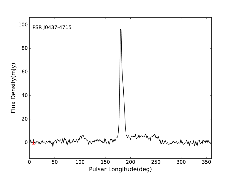
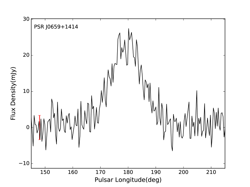
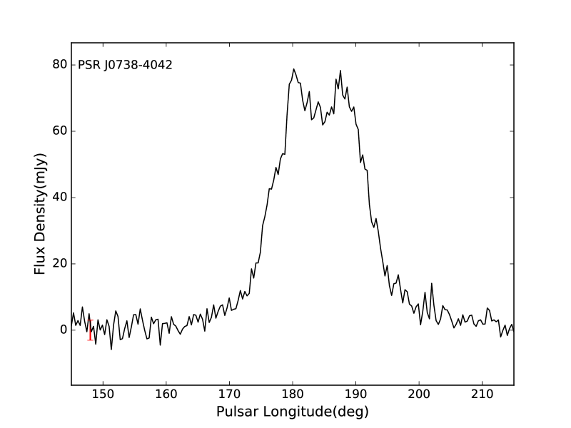
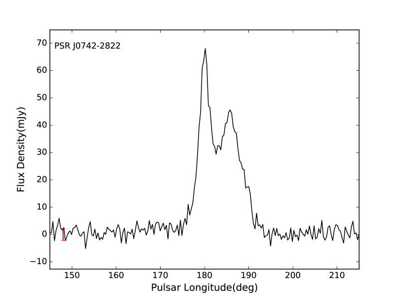
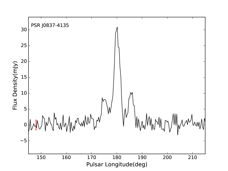
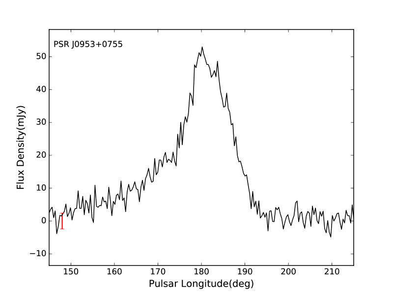
Figure 1: Integrated pulse profiles at 8.6 GHz obtained using the TMRT for 26 pulsars. The red bar represents $\pm\sigma_{b}$, the rms baseline noise. Except for PSRs J0437$-$4715 and J1705$-$1906, where there are 256 bins across the pulse period, all profiles have 1024-bins/period resolution.

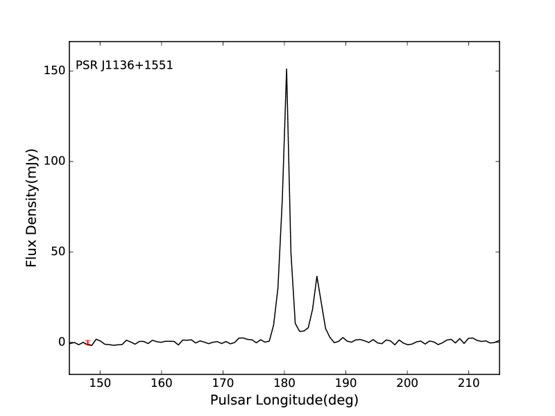
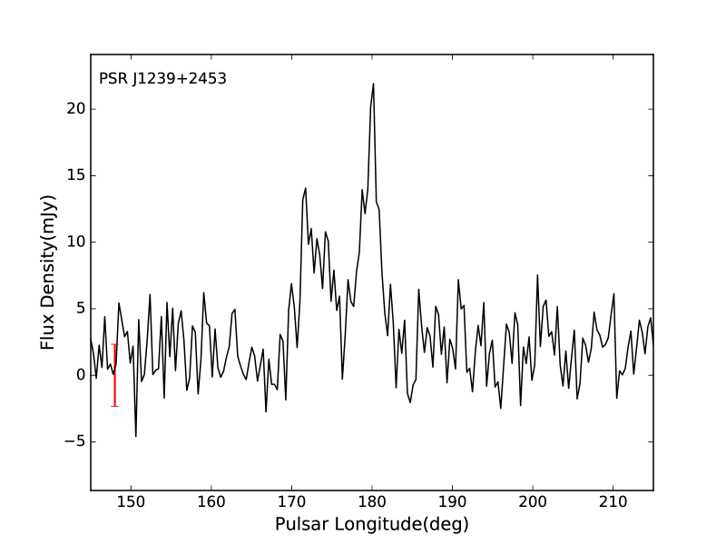
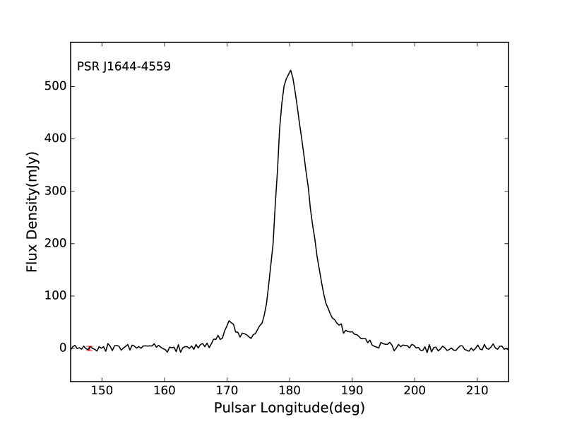
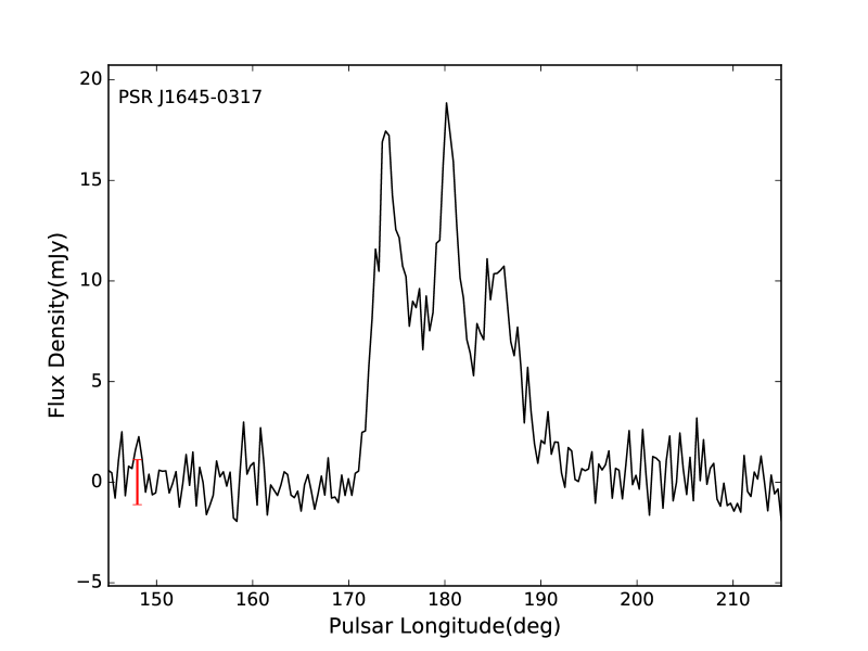
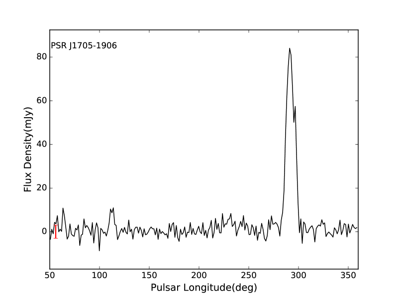
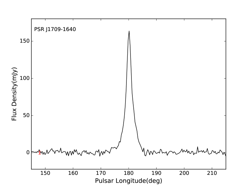
Figure 1: - continued

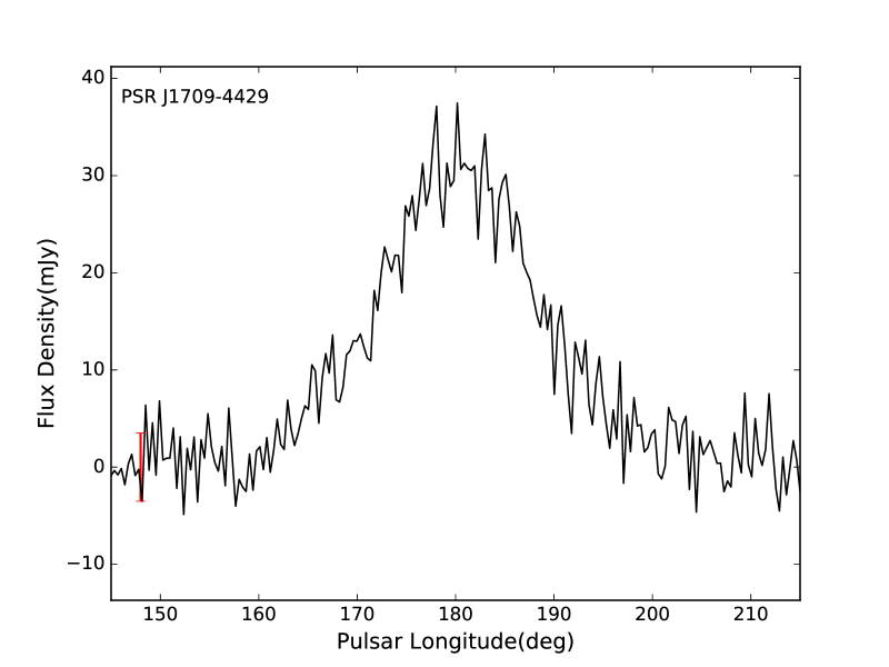
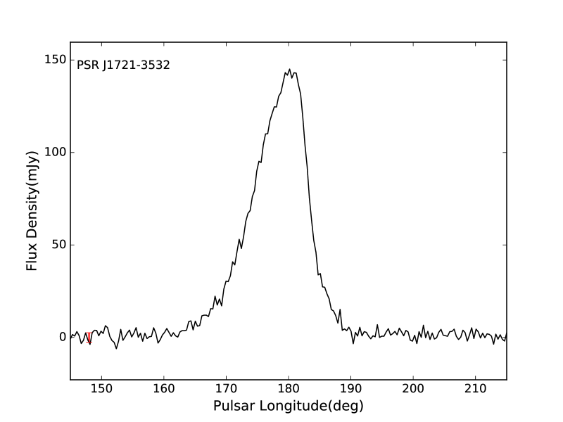
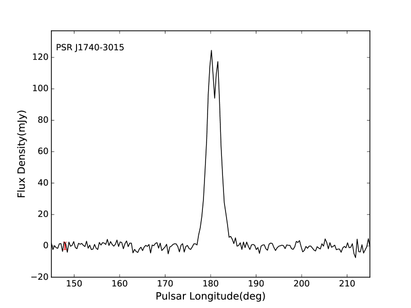
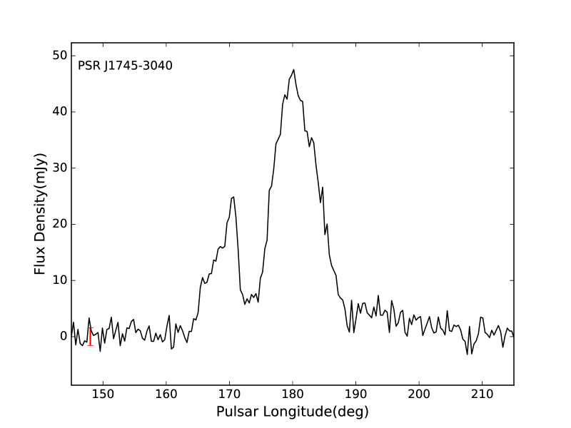
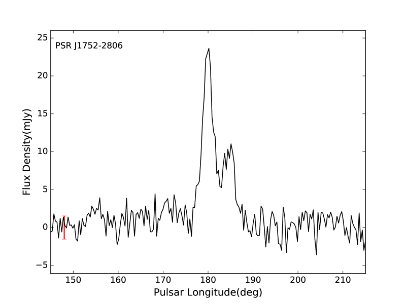
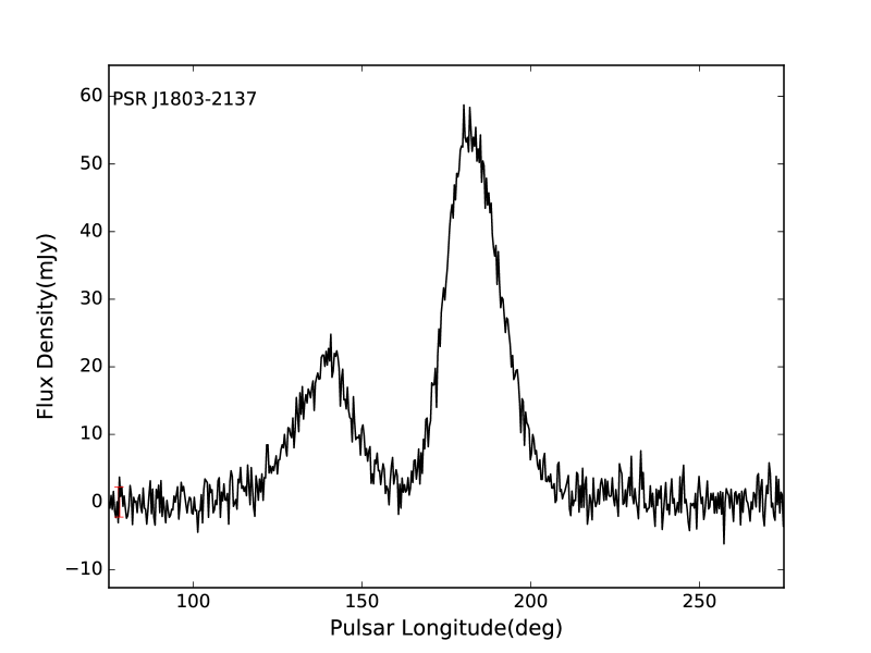
Figure 1: continued

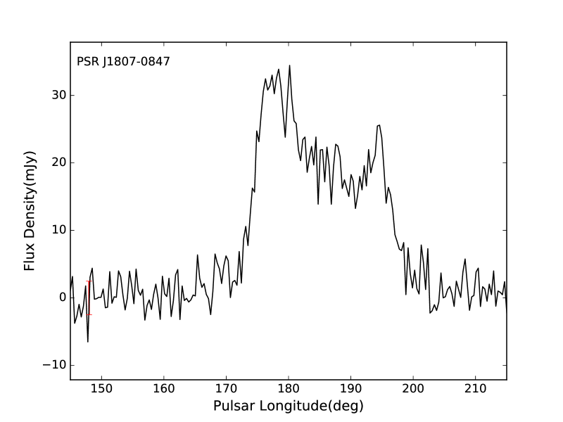
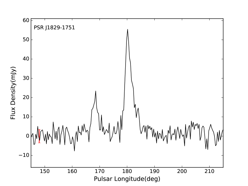
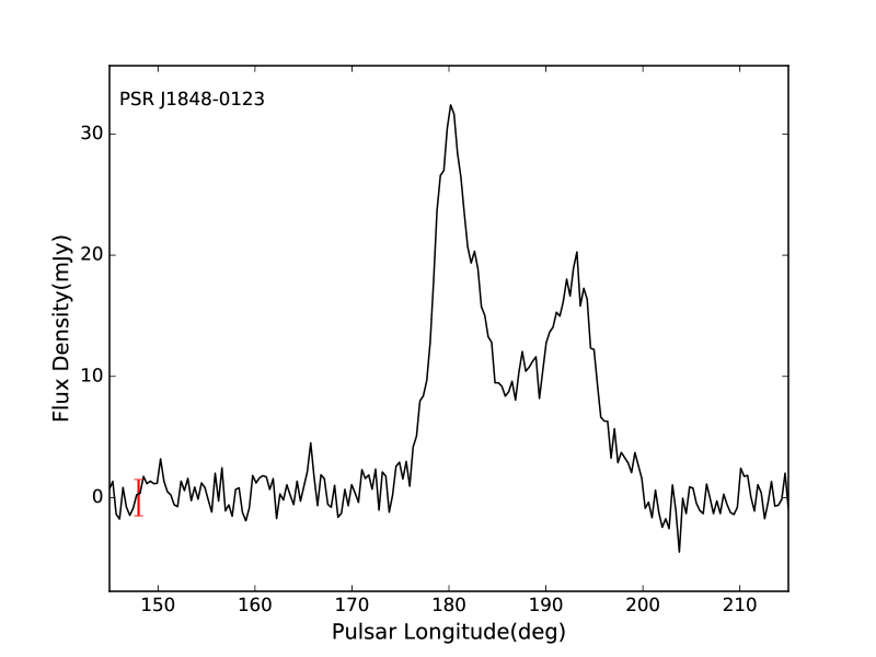
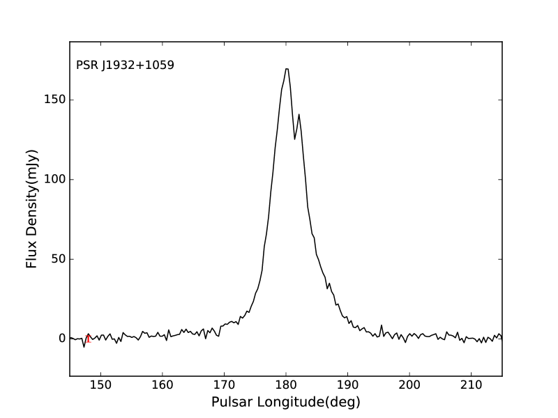
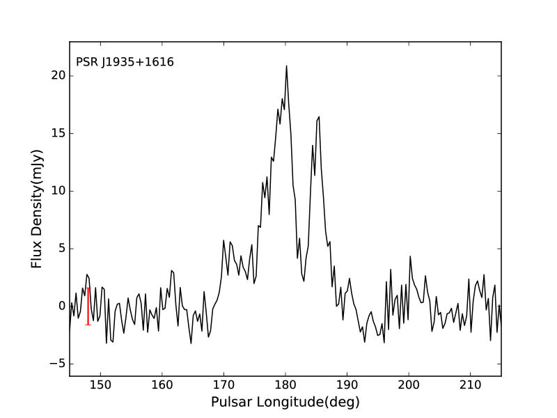
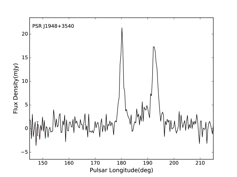
Figure 1: - continued

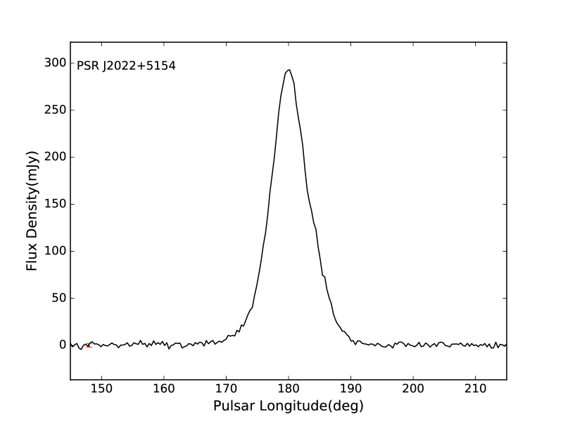
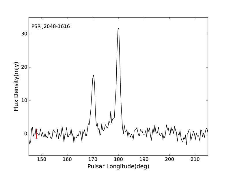
Figure 1: - continued

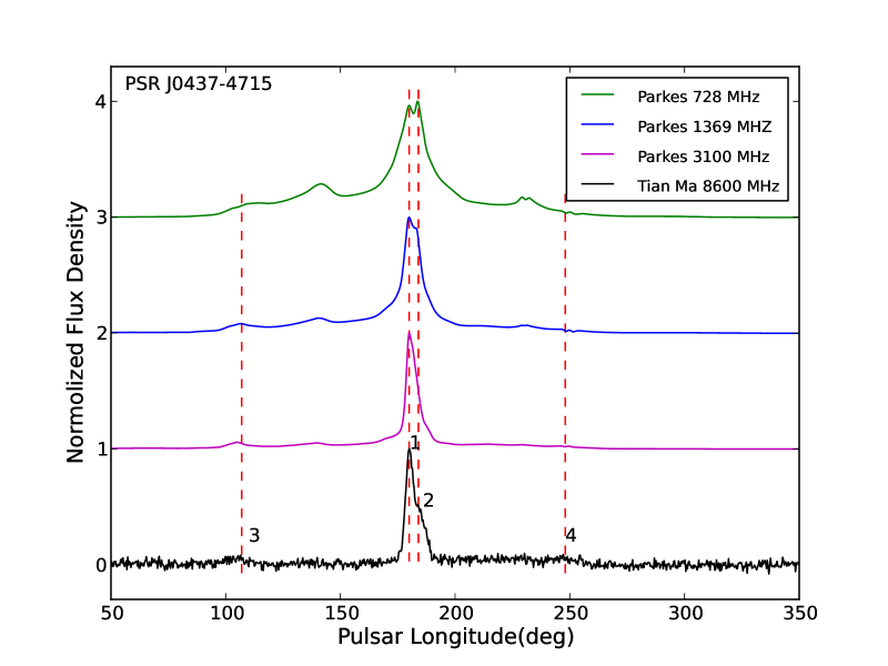
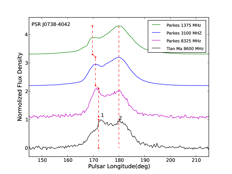
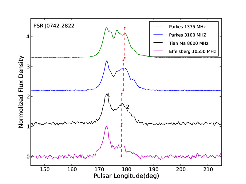
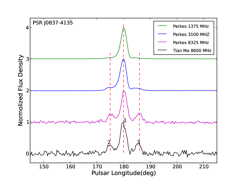
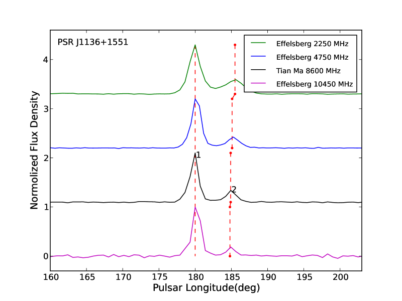
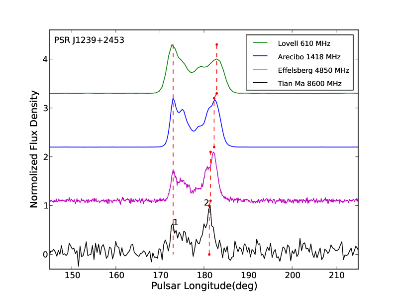
Figure 2: Observed integrated pulse profiles for 19 pulsars at four frequencies: 8.6 Hz from the TMRT and three other frequencies from the EPN profile database. Components are labelled on the TMRT profiles and corresponding components are connected by dashed lines.

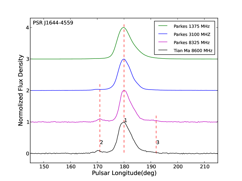
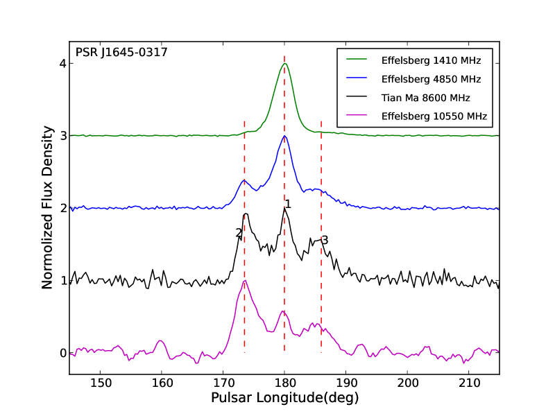
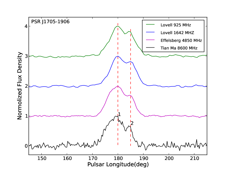
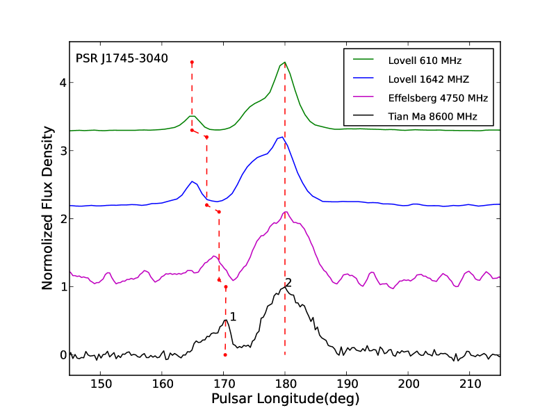
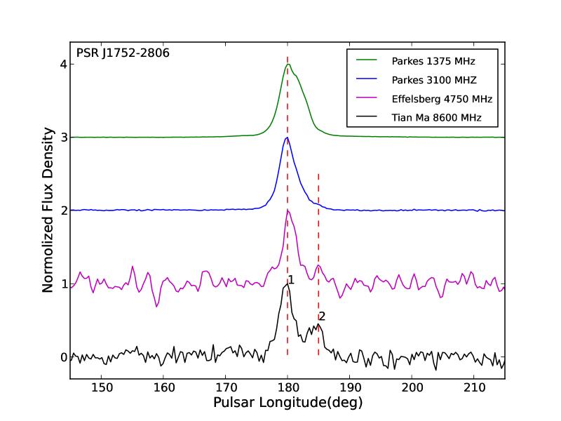
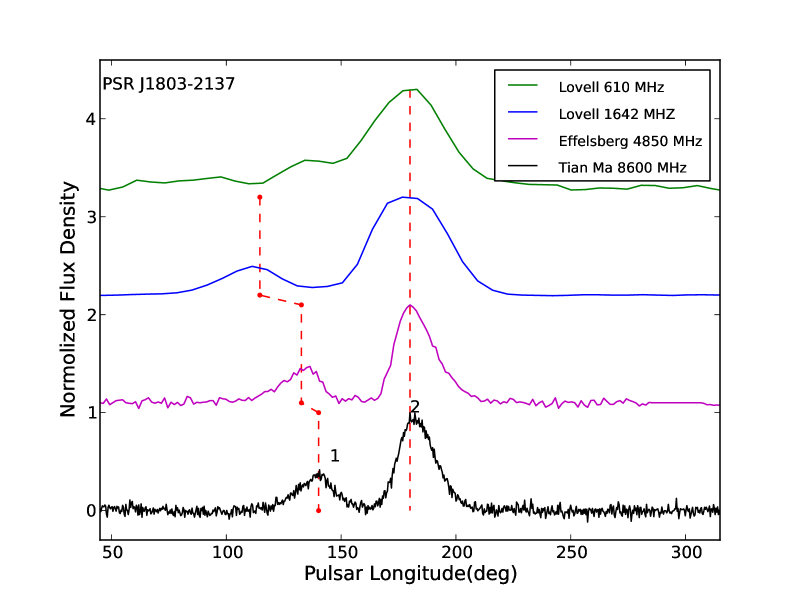
Figure 2: - continued

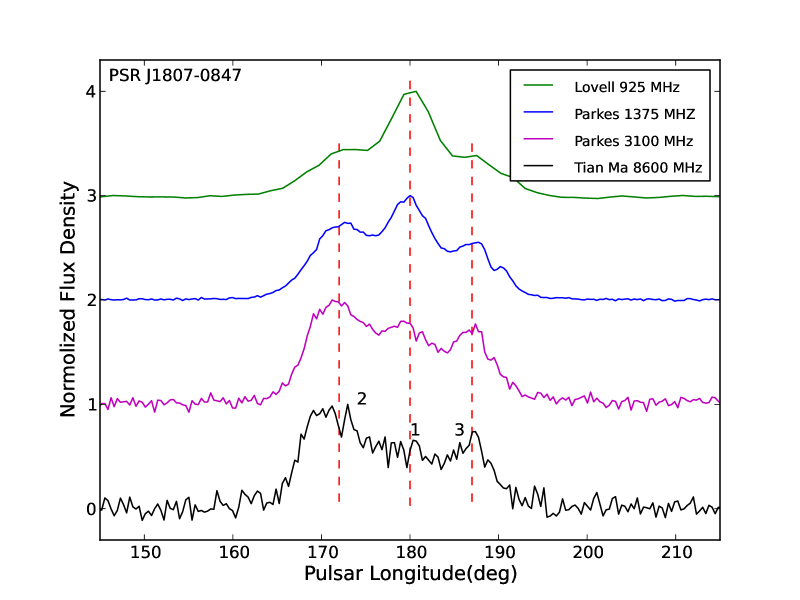
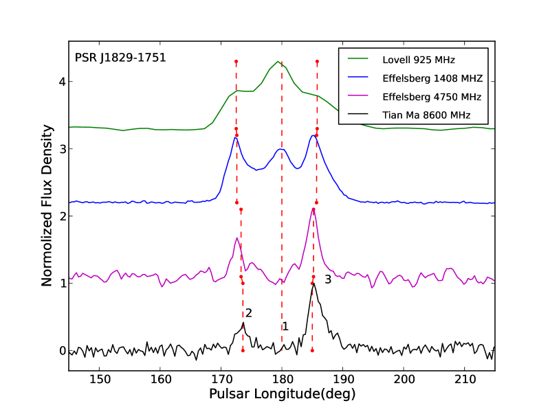
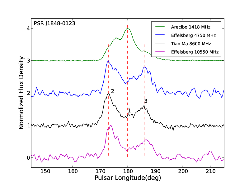
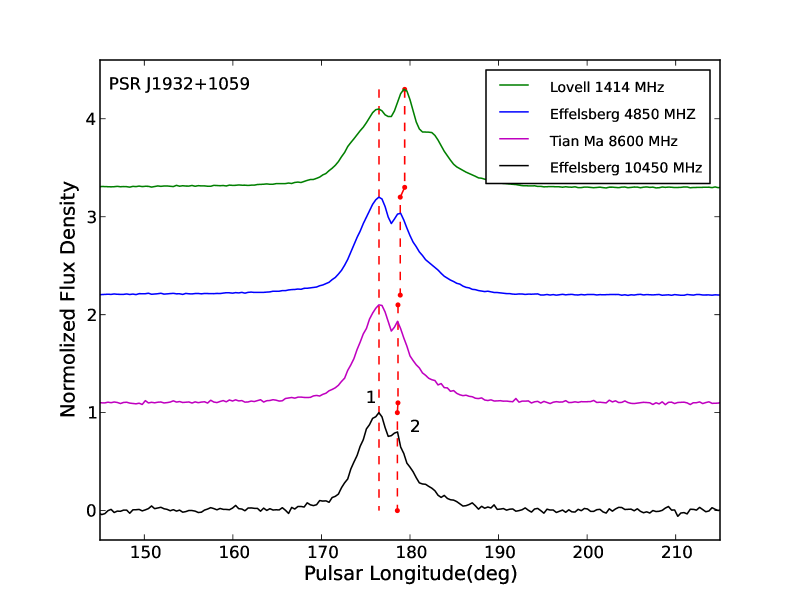
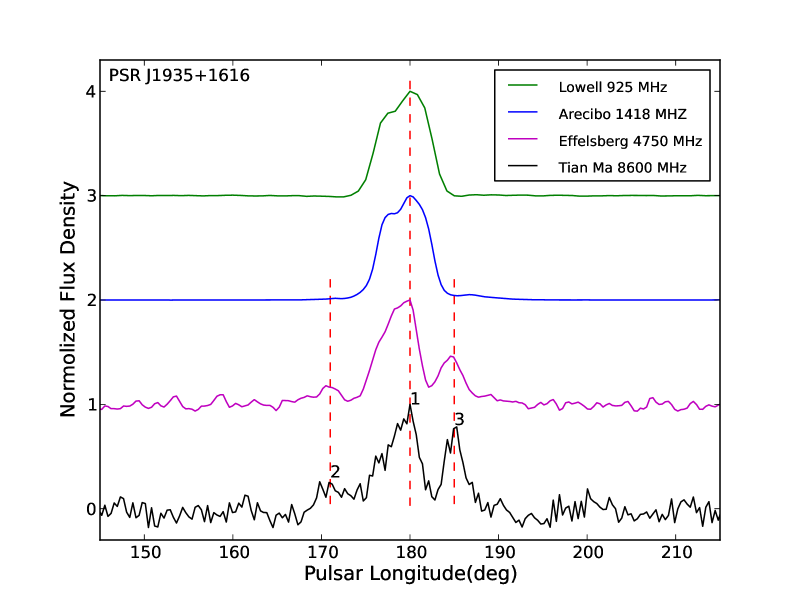
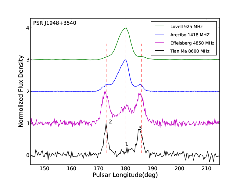
Figure 2: - continued

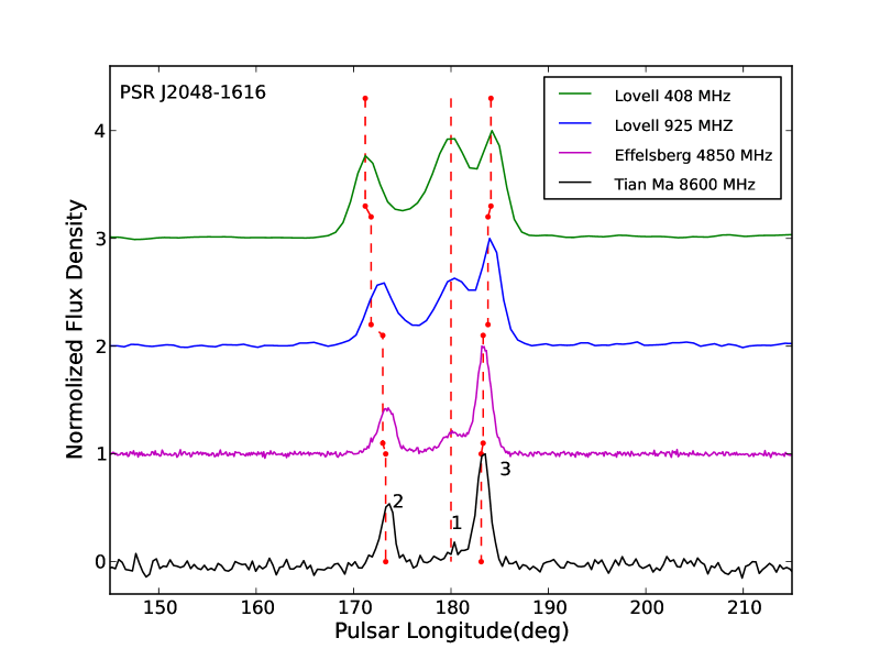
Figure 2: - continued

In this section we present the integrated pulse profiles for the 26 pulsars observed by TMRT and discuss their properties. Observational and profile parameters are given in Table 1. The first four columns give the pulsar J2000 name, the pulsar period, the observation date as a Modified Julian Day (MJD) and the on-source time. The next three columns give the separation between the outermost components with number of components in parenthesis and the observed pulse widths at 50% and 10% of the profile peak, all in units of degrees of pulse phase. Uncertainties are estimated for $W_{50}$ but not for $W_{10}$ which is often just approximate because of the low signal to noise ratio. For all the $W_{50}$ estimates, the S/N at 50% of the peak amplitude is greater than 3. For the $W_{10}$ measurements, the S/N at 10% of the peak amplitude is greater than 3 for 10 of the 26 pulsars. In Table 1, those with S/N between 1 and 3 are marked by ‘?’ and the value is rounded to the nearest degree. For the two (PSRs J0659+1414 and J1239+2453) with S/N $<1$, the $W_{10}$ measurement is omitted. The next two columns give the measured 8.6 GHz mean and peak flux densities. For comparison, the next three columns give pulse widths and flux densities at frequencies close to 8 GHz as measured by others. For 11 pulsars (PSRs J0437$-$4715, J1239$+$2453, J1645$-$0317, J1705$-$1906, J1745$-$3040, J1803$-$2137, J1807$-$0847, J1829$-$1751, J1848$-$0123, J1948$+$3540 and J2048$-$1616), these are the first published profiles for frequencies around 8 GHz. For 4 pulsars (PSRs J0742-2822, J1709-1640, J1932+1059 and J2022+5154), these profiles have a much better signal-to-noise ratio than previous observations (cf., Kramer et al., 1997b; Johnston et al., 2006). Figure 1 gives 8.6 GHz pulse profiles for the 26 pulsars observed by TMRT and Figure 2 compares the TMRT 8.6 GHz profiles with profiles at other frequencies obtained from the EPN profile database. The relationship of components at the different frequencies is indicated by dashed lines where the power-law frequency dependences of component phase discussed in §4.1 are assumed.

Table 1: Parameters for the 26 pulsars observed with the TMRT

PSR J2000	$P$	MJD	$T$	$\Delta\phi(N)$	$W_{50}$	$W_{10}$	$S_{8.6}\pm\sigma_{\rm S}$	$S^{\rm pk}_{8.6}\pm\sigma_{\rm b}$	$W_{50}^{\dagger}$	$W_{10}^{\dagger}$	$S^{\dagger}$
Name	(ms)	(d)	(min)	(deg)	(deg)	(deg)	(mJy)	(mJy)	(deg)	(deg)	$S_{8.35}$(mJy)	$S_{8.7}$(mJy)
J0437$-$4715	5.8	57156.203	30	143.0(4)	6.3$\pm 0.1$	13.9	5.24$\pm 0.12$	162.4$\pm 4.0$	$-$	$-$	$-$	$-$
J0659$+$1414	384.9	57156.533	30	$-$(1)	12.7$\pm 1.5$	$-$	0.96$\pm 0.11$	27.4$\pm 3.4$	11.81	261	2.51	$-$
J0738$-$4042	374.9	57156.370	30	7.7(2)	15.9$\pm 0.6$	27?	3.69$\pm 0.09$	78.8$\pm 3.0$	14.91	241	7.01	$-$
J0742$-$2822	562.6	57156.305	30	5.6(2)	8.9$\pm 0.2$	14.2	1.39$\pm 0.07$	68.1$\pm 2.2$	1.91	141	1.61	$0.55^{3}$
J0837$-$4135	751.6	57398.667	120	11.0(3)	2.9$\pm 0.1$	13?	0.39$\pm 0.05$	30.9$\pm 1.6$	2.51	131	1.31	$-$
J0953$+$0755	253.1	57156.419	30	$-$(1)	12.7$\pm 0.6$	30?	2.31$\pm 0.08$	53.0$\pm 2.4$	11.91	301	4.31	$0.58^{3}$
											$1.09\pm 0.22^{4}$	$-$
J1136$+$1551	1188.0	56863.411	50	5.1(2)	1.4$\pm 0.01$	$\,\ 7.3$	0.86$\pm 0.05$	151.2$\pm 1.1$	1.41	81	0.61	$0.62^{3}$
											$0.73\pm 0.15^{4}$	$-$
											$0.79\pm 0.16^{4}$	$-$
											$0.88\pm 0.18^{4}$	$-$
											$0.92\pm 0.18^{4}$	$-$
J1239$+$2453	1382.4	57156.463	30	8.3(2)	9.7$\pm 0.2$	$-$	0.31$\pm 0.07$	21.9$\pm 2.3$	$-$	$-$	$-$	$-$
J1644$-$4559	455.1	57156.668	30	20.6(3)	5.7$\pm 0.04$	11.9	10.20$\pm 0.12$	531.3$\pm 4.0$	5.11	161	2.21	$-$
J1645$-$0317	387.6	57398.882	120	12.3(3)	13.8$\pm 0.8$	19?	0.50$\pm 0.03$	18.8$\pm 1.1$	$-$	$-$	$-$	$-$
J1705$-$1906	298.9	57156.582	30	5.6(2)	11.2$\pm 0.4$	16?	1.17$\pm 0.09$	42.0$\pm 1.5$	$-$	$-$	$-$	$-$
J1709$-$1640	166.8	57156.828	30	$-$(1)	2.1$\pm 0.03$	$\,\ 6.5$	1.41$\pm 0.07$	163.8$\pm 2.2$	3.72	9.72	$-$	0.243
J1709$-$4429	102.5	57156.689	30	$-$(1)	15.9$\pm 1.5$	31?	1.75$\pm 0.11$	37.5$\pm 3.5$	16.71	321	5.51	$-$
J1721$-$3532	280.4	57156.753	30	$-$(1)	9.5$\pm 0.2$	19.9	4.30$\pm 0.08$	145.1$\pm 2.5$	8.81	171	1.91	$-$
J1740$-$3015	226.5	57156.774	30	1.2(2)	3.3$\pm 0.1$	$\,\ 6.0$	1.21$\pm 0.07$	124.5$\pm 2.5$	3.81	81	0.51	$-$
J1745$-$3040	367.4	57156.795	60	9.5(3)	14.2$\pm 0.3$	22.9	1.55$\pm 0.05$	47.6$\pm 1.6$	$-$	$-$	$-$	$-$
J1752$-$2806	529.2	57399.095	60	5.0(2)	2.8$\pm 0.2$	11?	0.30$\pm 0.05$	23.6$\pm 1.5$	2.51	121	0.91	$-$
J1803$-$2137	133.7	57156.873	30	40.2(2)	23.4$\pm 0.6$	81?	4.42$\pm 0.07$	58.7$\pm 2.2$	$-$	$-$	$-$	$-$
J1807$-$0847	163.7	57156.894	30	16.4(3)	20.9$\pm 0.6$	26?	1.56$\pm 0.08$	34.4$\pm 2.5$	$-$	$-$	$-$	$-$
J1829$-$1751	307.1	57157.609	30	11.3(2)	2.7$\pm 0.2$	18?	0.69$\pm 0.11$	55.4$\pm 3.5$	$-$	$-$	$-$	$-$
J1848$-$0123	659.4	57157.630	60	12.8(3)	15.3$\pm 0.3$	21?	0.87$\pm 0.05$	32.4$\pm 1.5$	$-$	$-$	$-$	$-$
J1932$+$1059	653.1	57156.890	30	2.2(2)	6.1$\pm 0.1$	14.9	3.62$\pm 0.06$	169.6$\pm 2.0$	6.62	14.52	$-$	$1.2^{3}\,\$
J1935$+$1616	358.7	57399.231	60	14.3(3)	9.7$\pm 0.3$	18?	0.43$\pm 0.05$	20.9$\pm 1.6$	$-$	$-$	$-$	0.183
J1948$+$3540	717.3	57156.974	60	12.4(3)	14.7$\pm 0.2$	17?	0.30$\pm 0.05$	21.3$\pm 1.5$	$-$	$-$	$-$	$-$
J2022$+$5154	606.9	57157.017	30	$-$(1)	6.7$\pm 0.04$	14.1	6.31$\pm 0.06$	293.0$\pm 2.0$	6.62	13.82	$1.73\pm 0.35^{4}$	2.843
J2048$-$1616	1961.0	57399.274	60	9.8(3)	10.9$\pm 0.2$	13?	0.30$\pm 0.04$	31.8$\pm 1.4$	$-$	$-$	$-$	$-$

^† Previously published results: 1: Johnston et al. (2006), 2: Kramer et al. (1997b), 3: Morris et al. (1981), 4: Maron et al. (2013)
$?$ $W_{10}$ estimate has low S/N.

PSR J0437$-$4715. Since its discovery by Johnston et al. (1993), PSR J0437$-$4715 has been extensively studied as the closest and brightest binary millisecond pulsar. Navarro et al. (1997) found that there are at least 10 pulse components in the profile and observed a frequency-dependent lag of the total-intensity profile with respect to the polarization profile. Yan et al. (2011) showed that multiple overlapping components cover at least 85% of the rotation period at 1.3 GHz. The integrated pulse profile at 8.6 GHz in Fig. 1 shows over-lapping central components and weaker emission on both sides to outlying components around $104\arcdeg$ and $250\arcdeg$. On the trailing side especially, there is a bridge of emission between the central and outlying component. Fig. 2 shows that the trailing central component 2 has a steeper spectrum than the leading component 1 and that the component separation is essentially independent of frequency (cf., Dai et al., 2015). At 8.6 GHz the center components are more dominant and the side components (around $140\arcdeg$ and $230\arcdeg$) are relatively weaker than the components at $104\arcdeg$ and $250\arcdeg$.

PSR J0659$+$1414 (B0656$+$14). This pulsar is a nearby middle-aged pulsar that is a strong source of pulsed high-energy emission (Weltevrede et al., 2010). In the radio band, Weltevrede et al. (2006) found that profile instabilities are caused by very bright and narrow pulses which may be related to the pulses observed from RRATs (Rotating Radio Transients). The TMRT 8.6 GHz pulse profile shown in Fig. 1 has relatively low S/N but is similar to the 8.4 GHz of Johnston et al. (2006). This pulsar has a single component profile at all radio frequencies (Lorimer et al., 1995; von Hoensbroech, 1999) and gets narrower with increasing frequency.

PSR J0738$-$4042 (B0736$-$40). Our 8.6 GHz profile for this pulsar shown in Fig. 1 has two obvious components and a third overlapping component on the leading edge. As Fig. 2 shows, this leading component is not as obvious in the 8.4 GHz Parkes profile of Johnston et al. (2006). Systematic variations in the leading components of the pulse profile at frequencies around 1.4 GHz that are related to changes in spin-down rate have been found for this pulsar (Karastergiou et al., 2011; Brook et al., 2014). It is likely that the differences in the 8 GHz profiles are related to the changes seen at lower frequencies.

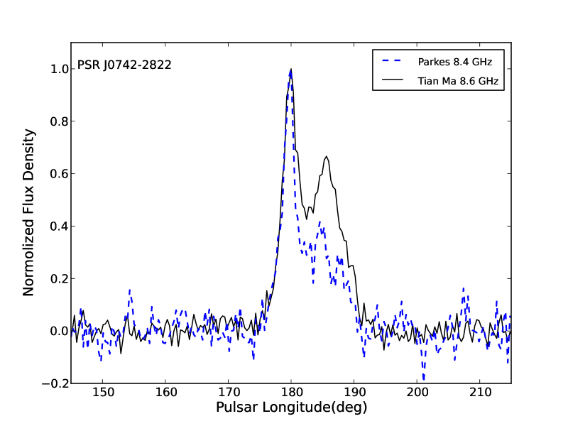
Figure 3: Comparison of Parkes and TMRT 8.6 GHz integrated profiles for PSR J0742-2822

PSR J0742$-$2822 (B0740$-$28). At 8.6 GHz the profile (Fig. 1) has two clear components. At lower frequencies, the pulsar consists of as many as seven components (Kramer et al., 1994) but the weaker ones are not visible in the TMRT profile. The width of pulse profile is almost the same over a wide frequency range (Chen & Wang, 2014). In observations at 1.4 GHz and 3.1 GHz (Keith et al., 2013), this pulsar has an interesting mode-changing behaviour on timescales of several hundred days that appears to be modified by a glitch. In the more common Mode I the trailing component is relatively weaker than in the less common Mode II. Fig. 3 shows that the TMRT profile differs from the 8.4 GHz profile of Johnston et al. (2006) in the same way as for the two modes observed at lower frequencies. Evidently the Parkes data were taken when the pulsars was in Mode I, whereas the pulsar was in Mode II during the TMRT observations.

PSR J0837$-$4135 (B0835$-$41). This pulsar was discovered at 408 MHz by Large et al. (1968) and Wang et al. (2001) used the Nanshan radio telescope at Xinjiang Astronomical Observatory to update the period and period derivative. The 8.6 GHz profile for this pulsar (Fig. 1) has a strong central component with outlier components on each side. As Fig. 2 shows, the frequency evolution of the profile shows classical behaviour with the outlier components having flatter spectra so that at 1.4 and 3.1 GHz the central component completely dominates the profile (Karastergiou & Johnston, 2006). The separation of the components in longitude is only weakly dependent on frequency.

PSR J0953$+$0755 (B0950$+$08). This famous pulsar, one of the original four pulsars discovered at Cambridge (Pilkington et al., 1968), has been extensively studied over a wide frequency range. The profile has a weak interpulse and bridge emission with the separation of the main component and interpulse close to $150\arcdeg$ over a wide frequency range (Hankins & Fowler, 1986). At low frequencies, the main pulse has two distinct components (Pilia et al., 2016) but at higher frequencies there is just one peak with an extension on the leading side. The 8.6 GHz profile shown in Fig. 1 has this form. Giant pulses and microstructure have been detected at different frequencies (Hankins, 1971; Cairns et al., 2004; Tsai et al., 2016).

PSR J1136$+$1551 (B1133$+$16). This is another of the original four pulsars discovered at Cambridge (Pilkington et al., 1968) that has a classic two-component profile and has been studied at many different frequencies. At low radio frequencies, the two components are of comparable amplitude (Bilous et al., 2016) but, as Fig. 1 shows, at 8.6 GHz, the trailing component is much weaker, indicating a much steeper spectrum. Thorsett (1991) has shown that the component separation $\Delta\phi$ for most double profiles can be fitted by the function of the form:

$$\Delta\phi=A\nu^{-\beta}+\Delta\phi_{\rm min}.$$ (6)

where $\nu$ is in MHz. For PSR J1136$+$1551, fitting to data at frequencies between 26 MHz and 10 GHz gives $A=53\arcdeg$, $\beta=0.50$ and $\Delta\phi_{\rm min}=4.4\arcdeg$. For 8.6 GHz, this equation gives $\Delta\phi=5.0\arcdeg$, in agreement with the measured value $5.1\arcdeg$ (Table 1).

PSR J1239$+$2453 (B1237$+$25). The mean pulse profile for this well-known bright pulsar has five distinct components at low radio frequencies and exhibits dramatic mode changing affecting mainly the central and trailing components (Srostlik & Rankin, 2005). The polarisation properties are consistent with a very small impact parameter, i.e., the magnetic axis passes within a fraction of one degree of the line of sight to the pulsar, so essentially a full diameter of the beam is traversed (Srostlik & Rankin, 2005). Fig. 2 shows that, at higher frequencies, the outer components more closely spaced. The component separation at 8.6 GHz is $8.3\arcdeg$ (Table 1), which is close to the $8.6\arcdeg$ predicted by Thorsett (1991) from a fit to data at frequencies between 80 and 4900 MHz. Fig. 2 also shows that, at 4.8 GHz and 8.6 GHz, the trailing component is stronger than the leading component, whereas the opposite is true at frequencies around and below 1 GHz. Clearly, of the two components, the trailing one has a flatter spectrum. Given the low S/N of the TMRT profile, it is not possible to identify systematic changes with frequency in the inner three components.

PSR J1644$-$4559 (B1641$-$45). This is the second brightest pulsar at 1.4 GHz and, at frequencies around 1 GHz, consists of an asymmetric primary component with a weak leading component (Manchester et al., 1980; Karastergiou & Johnston, 2006). At lower frequencies, the profile is broadened by interstellar scattering. Although the signal-to-noise ratio is low, Keith et al. (2011) showed that the leading component is nearly as strong as the main component at 17 GHz. Our 8.6 GHz profile (Fig. 1) and that of Johnston et al. (2006) clearly show the leading component and also a similar trailing component. The leading and trailing components both have relativly flat spectra and clearly are conal emission. Although we do not know the impact parameter, the relatively flat PA variation (Johnston et al., 2006) as well as the strong core component suggests it must be small so that the beam radius is probably about half of the separation of the leading and trailing components, i.e., close to $10\arcdeg/\sin\alpha_{B}$, where $\alpha_{B}$ is the magnetic inclination angle.

PSR J1645$-$0317 (B1642$-$03). As Fig. 2 shows, in terms of the pulse profile and its frequency dependence, PSR J1645$-$0317 is essentially a twin of PSR J1644$-$4559, except that the outlier conal components are relatively stronger and are evident at a lower frequency for PSR J1645$-$0317. At frequencies above 8.6 GHz, the leading component dominates the profile whereas the central component is weak, showing that it has a much steeper spectral index. The apparent beam radius is a little smaller than for PSR J1644$-$4559, about $6\arcdeg/\sin\alpha_{B}$.

PSR J1705$-$1906 (B1702$-$19). This pulsar has a relatively short period ($\sim 0.299$ s) and, at frequencies around 1 GHz, a strong interpulse separated from the main pulse by $180\arcdeg$ of longitude (Biggs et al., 1988). The observed polarisation variations can be interpreted in terms of an orthogonal rotator with the main pulse and interpulse from opposite poles (e.g., Karastergiou & Johnston, 2004). However, Weltevrede et al. (2007) find a $10P$ modulation in both the main pulse and interpulse that remains phase-locked over years, a result that is difficult to explain in the two-pole model.

Our observations at 8.6 GHz (Fig. 1, plotted with 256-bin/period resolution to improve the S/N) clearly shows the interpulse separated from the main pulse by $179\arcdeg\pm 1\arcdeg$ and with a peak flux density about 6% of that of the main pulse. The interpulse evidently has a spectrum relative to the main pulse which peaks around 1 GHz, with flux density ratios of approximately 0.20, 0.24 and 0.45 at 408 MHz, 610 MHz and 1.4 GHz respectively (Gould & Lyne, 1998), and 0.30 at 4.85 GHz (Kijak et al., 1998). At 8.6 GHz, Fig. 2 shows that the main pulse has at least two components and that the pulse profile changes little between frequencies of 900 MHz and 8.6 GHz.

PSR J1709$-$1640 (B1706$-$16). The 8.6 GHz pulse profile shown for this pulsar in Fig. 1 is dominated by a single strong component with a weak component at its leading edge. These components are also seen in the 4.75 GHz profile presented by Kramer et al. (1997b). Their 8.5 GHz profile is affected by systematic baseline noise and these weaker components are not visible. Chen & Wang (2014) show that the width of the main component decreases with increasing frequency, and our 8.6 GHz profile is consistent with that.

PSR J1709$-$4429 (B1706$-$44). PSR J1709$-$4429 is a young Vela-like pulsar that shows both high-energy emission (e.g., Abdo et al., 2010) and intermittent strong micropulses from a small phase range near the trailing edge of the pulse profile (Johnston & Romani, 2002). The radio pulse profile is simple with one dominant component and is highly linearly polarised (Qiao et al., 1995; Johnston et al., 2006). Our 8.6 GHz pulse profile is similar to that of Johnston et al. (2006), showing a single component of 50% width about $16\arcdeg$ of longitude. This is significantly narrower than the 50% width, about $21\arcdeg$, at 1.4 GHz (Hobbs et al., 2004).

PSR J1721$-$3532 (B1718$-$35). This pulsar has a relatvely short pulse period ($\sim 280$ ms) and a very high dispersion measure (496 cm^-3 pc) (Hobbs et al., 2004). At 8.6 GHz, Fig. 1 shows that this pulsar has a simple but asymmetric profile with a slow rising edge and a steeper falling edge (cf., Johnston et al., 2006). At 1.4 GHz, the profile is highly scattered (Hobbs et al., 2004) with a 1 GHz scattering timescale of about 78 ms (Johnston, 1990).

PSR J1740$-$3015 (B1737$-$30). This pulsar is young (characteristic age about 20,000 years) and has a large surface-dipole magnetic field ($\sim 1.7\times 10^{13}$ G). Its main claim to fame is the high rate of glitch occurrence, with more than 30 observed at an average rate of about one per year (Espinoza et al., 2011, and the ATNF Pulsar Catalogue Glitch Table). At frequencies around 1 GHz, the profile for this pulsar is dominated by a single component (e.g., Gould & Lyne, 1998) but as Fig. 1 shows, at 8.6 GHz the peak of the profile splits into two components. Parkes observations at a similar frequency (Keith et al., 2011) show the same profile shape. Above 1 GHz, the profile 50% width is approximately constant (Chen & Wang, 2014), but at lower frequencies it is affected by interstellar scattering (Krishnakumar et al., 2015).

PSR J1745$-$3040 (B1742$-$30). Fig. 1 shows that at 8.6 GHz this pulsar has a two-component profile, with a component separation of slightly less than $10\arcdeg$ (Table 1). Fig. 2 shows that, toward lower frequencies, the leading component becomes relatively weaker, a central component appears and the separation between the leading and trailing components increases greatly (cf., Gould & Lyne, 1998).

PSR J1752$-$2806 (B1749$-$28). This strong pulsar, discovered by Turtle & Vaughan (1968), lies within $2\arcdeg$ of the Galactic Centre. At frequencies of a few GHz the pulse profile is dominated by a single component. At frequencies below about 400 MHz, profile broadening due to interstellar scattering is evident (Alurkar et al., 1986). Fig. 1 shows that at 8.6 GHz there is a trailing component with a peak flux density about 40% that of the leading component. This trailing component can be seen at 3.1 GHz and 4.75 GHz (Fig. 2), becoming relatively weaker with decreasing frequency. At frequencies around 1 GHz, a central, probably core, component is visible.

PSR J1803$-$2137 (B1800$-$21). This young Vela-like pulsar has an extraordinarily wide double profile with $W_{10}$ at 1.4 GHz of 43 ms or $115\arcdeg$ of longitude (Hobbs et al., 2004). The spectrum has a peak at around 1 GHz with a variable low-frequency spectrum probably due to varying interstellar absorption (Basu et al., 2016).

At 8.6 GHz, Fig. 1 shows that the profile retains its wide-double form. $W_{10}$ is $81\arcdeg$ (Table 1) showing that the component separation is a strong function of frequency. Fig. 2 illustrates this and shows that the leading component has a relatively flatter spectrum, being barely visible at 610 MHz (cf., Basu et al., 2016) and becoming prominent at higher frequencies. At low frequencies, a central core component also becomes evident.

PSR J1807$-$0847 (B1804$-$08). At frequencies around 1 GHz, this pulsar has a clear three-component pulse profile (e.g.. Hobbs et al., 2004). As shown in Fig. 1, at 8.6 GHz the profile has a classic double form with a steep outer edges and a connecting bridge of emission. Fig. 2 shows that the central component has a steeper spectrum and this along with its central location marks it as a core component. There is no significant frequency dependence of component separation.

PSR J1829$-$1751 (B1826$-$17). At 8.6 GHz Fig. 1 shows that the mean pulse profile has two isolated components, with the trailing one about twice as strong as the leading one. However, at 0.925 and 1.408 GHz (Fig. 2; Gould & Lyne, 1998), a central core component is clearly visible and the leading and trailing components are of comparable strength, indicating a wide variation in spectral index across the profile. Overall, the profile frequency evolution is very similar to that of PSR J1807$-$0847, although there is a more significant narrowing of the profile width with increasing frequency for PSR J1829$-$1751.

PSR J1848$-$0123 (B1845$-$01). Our 8.6 GHz profile has two components with a bridge between them (Fig. 1). Fig. 2 shows that the profile frequency evolution in this pulsar is very similar to the preceding two pulsars, with a central core component becoming dominant at frequencies around 1.4 GHz. There is little change in pulse width between 1 GHz and 10 GHz.

PSR J1932$+$1059 (B1929$+$10). This is a nearby, bright and isolated pulsar which has a relatively weak interpulse preceding the main pulse by about $170\arcdeg$ of longitude (e.g., Stairs et al., 1999). At low frequencies, emission can be seen over most of the pulse period allowing detection of a double-notch feature trailing the main pulse by about $100\arcdeg$ of longitude (McLaughlin & Rankin, 2004). This feature similar to those seen in PSR J0437$-$4715 and PSR J0953$+$0755 (B0950$+$08) which also have detectable emission over most of the pulse period. At 8.6 GHz the profile has broad wings and two identifiable components near the profile peak (Fig. 1). The multi-frequency profiles in Fig. 2 (see also Hankins & Rickett, 1986) show that the leading component has a flatter spectrum than the central and trailing components. At 1.4 GHz the main pulse has a 50% width of about $12\arcdeg$ (Hobbs et al., 2004), whereas at 8.6 GHz the pulse is much narrower with $W_{50}$ about $6\arcdeg$ (Table 1).

PSR J1935$+$1616 (B1933$+$16). Sieber et al. (1975) showed the frequency evolution in this profile from a single dominant component at 430 MHz to three components above 2 GHz. This is a classic core-conal structure with the core region dominating at low frequencies and conal outriders appearing at higher frequencies. Our 8.6 GHz profile (Fig. 1) shows that this evolution continues to higher frequencies, with the central and trailing components of comparable strength while the leading component is stronger than at lower frequencies (Fig. 2) but only about 30% as strong as the other two components. The higher S/N profiles at 925 MHz (Gould & Lyne, 1998) and 1418 MHz (Weisberg et al., 1999) given in Fig. 2 show that the core emission consists of two overlapping components. This is consistent with the gradual evolution from core emission to conal emission across the profile discussed by Lyne & Manchester (1988).

PSR J1948$+$3540 (B1946$+$35). Even more than PSR J1935$+$1616 discussed above, PSR J1948$+$3540 shows the evolution from core-dominated at low frequencies to cone-dominated at high frequencies (Fig. 2). The 8.6 GHz integrated pulse profile given in Fig. 1 has a basically double pulse profile although there is evidence for a weak central or core component. At least above 1 GHz, the pulse phases of three components and the overall pulse width are stable (Fig. 2).

PSR J2022$+$5154 (B2021$+$51). PSR J2022$+$5154 is one of the strongest pulsars at high frequencies with detections up to 43 GHz (e.g., Kramer et al., 1997a). At low frequencies, e.g., around 400 MHz, the profile is double-peaked with the trailing component about twice as strong as the leading one and a component separation of about $8\arcdeg$ (Gould & Lyne, 1998). Around 1.4 GHz, the leading component evidently disappears and the trailing component bifurcates to two overlapping components. Fig. 1 shows that, at 8.6 GHz, only a single component with a 50% width of $6.7\arcdeg$ (Table 1) is evident.

PSR J2048$-$1616 (B2045$-$16). This well known pulsar, discovered by Turtle & Vaughan (1968), has a triple component profile at frequencies of a few GHz and below and a position-angle swing indicating a traverse of the polar cap with low impact angle, i.e., the line of sight passing close to the magnetic axis (e.g., Manchester, 1971). Fig. 1 shows that at 8.6 GHz the central component has almost disappeared. It therefore has a steeper spectrum and is consistent with core emission despite being offset from the profile centre (cf., Lyne & Manchester, 1988). Fig. 2 shows that the trailing component becomes relatively stronger at high frequencies and that the component separation is a decreasing function of frequency (cf., Chen & Wang, 2014).

4 Discussion

Pulsar integrated profiles come in many different forms with different numbers of pulse components, different separations, sometimes interpulses and different spectral behaviour for the different components. In most cases, profiles and components are narrower and weaker at higher frequencies. These different behaviours give important information about the structure of pulsar emission regions and the radiation mechanisms.

Even though there are very many observations of integrated pulse profiles, the sample at high frequencies is relatively limited, largely because of the typically steep spectrum of pulsar emission. The 8.6 GHz observations of 26 pulsars reported here nearly double the number of published high-quality high-frequency pulse profiles.

4.1 Frequency dependence of profile widths

It has long been known that for most pulsars the profile width, or component separation for multiple-component pulsars, decreases with increasing radio frequency (e.g., Manchester & Taylor, 1977; Cordes, 1978), at least at frequencies below about 1 GHz. This was often modelled as a power law $\Delta\phi\sim\nu^{\beta}$ with $\beta$ typically about $-0.25$. At higher frequencies, pulse widths become more frequency-independent, leading to two-component power-law models with a break at some frequency, typically about 1 GHz (Slee et al., 1987). As discussed above in §3, an alternative model (Eq. 6) with a single power law combined with a minimum pulse width was shown by Thorsett (1991) to accurately describe the frequency dependence for many pulsars.

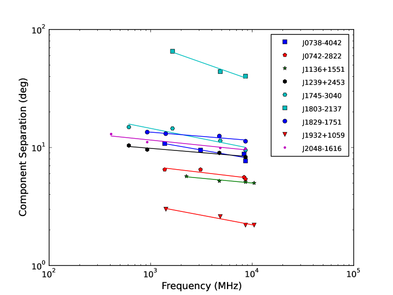
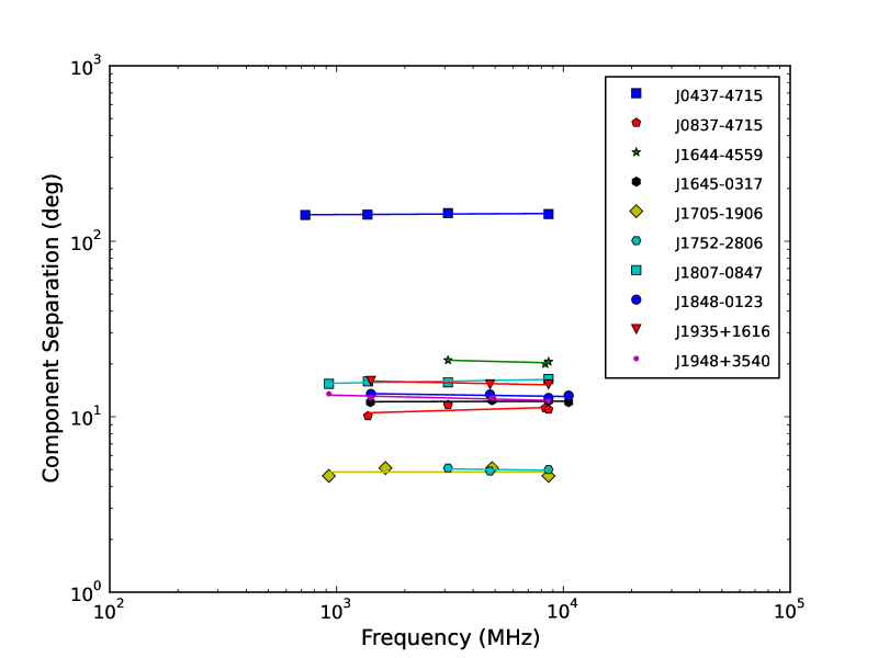
Figure 4: Separation of profile outermost components as a function of frequency for nine pulsars where the separation decreases with increasing frequency (left panel) and for ten pulsars with essentially constant component separation (right panel). The lines are the fitted power law for each pulsar.

Our 8.6 GHz observations add significantly to the available data on high-frequency pulse widths. Of the 26 pulsars, 19 have two or more clearly resolved components, allowing a measurement of $\Delta\phi$ as listed in Table 1. These component separations are compared with other measurements made over a range of frequencies (Seiradakis et al., 1995; von Hoensbroech & Xilouris, 1997; Gould & Lyne, 1998; Weisberg et al., 1999; Dai et al., 2015) in Fig. 4. The observed frequency dependencies are closely power-law and appear to divide into two groups, those with a signficant frequency dependence and those which are essentially frequency-independent. The frequency range fitted, the power-law indices ($\beta$) and the rms residuals from the fit ($\sigma$) are given in Table 2 for the first group and Table 3 for the second group. Table 3 also gives the mean separation of the outermost components, $\langle\Delta\phi\rangle$, for the pulsars with frequency-independent component separations. These power-law frequency dependencies are shown in Fig. 2 for each pulsar, with the phase of the dashed lines for each profile representing the predicted phase for the frequency of that profile.

Table 2: Power-law ($\nu^{\beta}$) indices for component separation for the nine pulsars with decreasing separation at higher frequencies.

PSR	Frequency	$\beta$	$\sigma$
Name	(MHz)		($\arcdeg$)
J0738$-$4042	1375$-$8600	$-0.15\pm 0.04$	0.4
J0742$-$2822	1375$-$10550	$-0.10\pm 0.03$	0.2
J1136$+$1551	2250$-$10450	$-0.09\pm 0.01$	0.1
J1239$+$2453	610$-$8600	$-0.07\pm 0.01$	0.2
J1745$-$3040	610$-$8600	$-0.17\pm 0.04$	0.9
J1803$-$2131	1642$-$8600	$-0.30\pm 0.05$	2.0
J1829$-$1751	925$-$8600	$-0.07\pm 0.02$	0.3
J1932$+$1059	1414$-$10450	$-0.18\pm 0.02$	0.1
J2048$-$1616	408$-$8600	$-0.09\pm 0.02$	0.5

Table 3: Power-law indices ($\nu^{\beta}$) for component separation the ten pulsars with essentially constant component separation at higher frequencies.

PSR	Frequency	$\beta$	$\sigma$	$\langle\Delta\phi\rangle$
Name	(MHz)		($\arcdeg$)	($\arcdeg$)
J0437$-$4715	728$-$8600	$0.01\pm 0.01$	1.2	141.5
J0837$-$4135	1375$-$8600	$0.04\pm 0.04$	0.6	11.3
J1644$-$4559	3100$-$8600	$-0.03\pm 0.03$	0.3	21.4
J1645$-$0317	1410$-$10550	$0.003\pm 0.009$	0.1	12.1
J1705$-$1906	925$-$8600	$0.00\pm 0.04$	0.3	4.9
J1752$-$2806	3100$-$8600	$-0.02\pm 0.04$	0.1	5.1
J1807$-$0847	925$-$8600	$0.02\pm 0.01$	0.2	15.6
J1848$-$0123	1418$-$10550	$-0.02\pm 0.01$	0.2	13.1
J1935$+$1616	1418$-$8600	$-0.03\pm 0.01$	0.1	15.2
J1948$+$3540	925$-$8600	$-0.01\pm 0.01$	0.2	12.8

Component separation indices for the first group range between $-0.07$ and $-0.3$, whereas for the second group they are generally $0.00\pm 0.03$. For the pulsars in the first group there is no sign of a flattening at the highest frequencies plotted and for those in the second group, there is no sign of a steepening for the lowest frequencies plotted. This is not necessarily inconsistent with earlier results that indicate a change of power-law index as this is only seen in a subset of all pulsars (e.g., Chen & Wang, 2014) and, when present, generally occurs around 1 GHz. Most of the plotted points are at frequencies higher than this.

Most magnetic-pole emission models interpret the decreasing profile width with increasing frequency in terms of radius-to-frequency apping (e.g., Cordes, 1978). Predicted indices range between $-0.14$ (Beskin et al., 1988) and $-0.45$ (Vitarmo & Jauho, 1973) with the well-known Ruderman & Sutherland (1975) model giving $-0.33$. Within the context of radius-to-frequency mapping, the flattening out at high frequencies is interpreted in terms of a lower limit to the altitude of the emission region, possibly at or close to the neutron-star surface (e.g., Kramer et al., 1997b).

Interestingly, Mitra & Rankin (2002) found from an analysis of multiple-component profiles that, while outer conal pairs followed the Thorsett (1991) frequency dependence of component separation, inner conal pairs did not and have an essentially frequency-independent component separation. A similar dependence of frequency dependence for inner and outer cones was found by Wu et al. (1998) for PSR B1451$-$68. These observations provide an alternate explanation for the two types of frequency dependence that we observed, namely that for the frequency-independent cases, the emission is from an inner cone. However, as Fig. 4 shows, the frequency-independent component separations are typically about the same as the frequency-dependent ones, which would not be expected if the former were inner cones. This simple comparison ignores the effects of line-of-sight impact parameter and magnetic inclination. Most of these pulsars show core emission, and so impact parameters should be small and have little effect. The effects of magnetic inclination are difficult to reliably quantify since most estimates are based on observed pulse widths and the assumption of a well-defined beam opening angle (Lyne & Manchester, 1988; Rankin, 1990). Another relevant point is that at least two of the frequency-independent group (PSRs J1807$-$0847 and J1848$-$0123) have multiple components and the frequency independence appears to extend across all components. Millisecond pulsars such as PSR J0437$-$4715 are also exceptional and are discussed below.

Most emission models assume that the radiation is emitted tangentially to the local magnetic field, giving a simple relation between the beam opening angle, the emission height and the radial position (from the magnetic axis) of the field line on the polar cap (e.g., Rankin, 1993; Mitra & Rankin, 2002). However, in the inverse Compton scattering (ICS) model (Qiao & Lin, 1998), the different conal components result from different beam angles relative to the field direction on a given field line. The ICS model can account for the different observed frequency dependence of component separations for inner and outer cones (Qiao et al., 2001).

For most millisecond pulsars (e.g., Dai et al., 2015), including PSR J0437$-$4715 described in §3, and some other pulsars with wide profiles, e.g., PSR J0953+0755 (B0950+08) also described in §3, the observed component separation is frequency independent. For these pulsars the emission region may be close to the light cylinder and caustic effects may be important in defining the observed profile shape (Ravi et al., 2010), thereby negating the effects of radius-to-frequency mapping and providing an alternative explanation for frequency-independent component separations.

Table 4: Spectral indices for leading, central and trailing components

PSR	$\alpha_{\rm l}$	$\alpha_{\rm c}$	$\alpha_{\rm t}$
Name
J0837$-$4135	$-1.3\pm 0.2$	$\,\ -2.2\pm 0.01$	$\,\ -1.3\pm 0.01$
J1645$-$0317	$-2.0\pm 0.2$	$-5.0\pm 0.2$	$-2.5\pm 0.3$
J1807$-$0847	$-1.0\pm 0.1$	$-1.5\pm 0.1$	$-1.2\pm 0.1$
J1829$-$1751	$-1.7\pm 0.2$	$-2.1\pm 0.2$	$-1.2\pm 0.1$
J1848$-$0123	$-1.4\pm 0.2$	$-1.9\pm 0.4$	$-1.5\pm 0.2$
J1948$+$3540	$-1.5\pm 0.1$	$-2.7\pm 0.1$	$-1.1\pm 0.1$
J2048$-$1616	$\,\ -1.9\pm 0.05$	$\,\ -2.3\pm 0.06$	$\,\ -1.6\pm 0.09$

4.2 Spectral properties of components in integrated pulse profiles

There is ample evidence that central and outer regions of observed pulse profiles have different spectral properties, with the central regions generally having steeper spectra (e.g., Rankin, 1983, 1993; Lyne & Manchester, 1988). Within the context of the magnetic-pole model, this is generally interpreted as differing properties for emission from the “core” and “conal” or outer regions of the emission cone. There is debate about whether the mechanism for the core and cone emission is different (Rankin, 1983) or basically the same with a gradation of properties across the polar cap (Lyne & Manchester, 1988).

In Table 4 we present spectral indices for the leading, centre and trailing components for the seven of our 26 pulsars where these components are clearly visible over a range of frequencies. These results combine data from our 8.6 GHz observations with the observations at other frequencies as used in the analysis of component separation (§4.1). Component flux densities were estimated by fitting Gaussian profiles to the relevant components at each frequency and taking the product of the component amplitude and width. This procedure gives a better estimate of the total component flux density since component widths tend to be greater at lower frequencies (cf., Wu et al., 1998).

In all seven cases, the spectral indices of the central components are close to or more negative than those of the leading and trailing components, further emphasizing this property of the pulsar emission mechanism. In some cases the spectral index difference is large. For example, for PSR J1645$-$0317 (B1642$-$03), the spectral index of the central component is $-5.0$ compared to a mean spectral index for the outer components of about $-2.3$.

4.3 Period dependence of core components

On the assumption that pulsar emission beams are bounded by the open field lines emanating from a polar cap, the observed pulse widths are determined by the altitude of the emission region relative to the light-cylinder radius, the line-of-sight impact parameter relative to the beam radius and the magnetic inclination angle $\alpha_{B}$ (e.g., Lyne & Manchester, 1988). To obtain beam radii, emission altitudes and magnetic inclination angles from these relations, the (linear) polarisation properties must be known. Rankin (1990) proposed a simpler relation based on the observed width of core components. If a gaussian beam profile is assumed for the components, then the observed half-power component width is independent of the impact parameter. Consequently, total-power measurements are sufficient. Rankin (1990) used the observed core-component half-power width $W_{50}^{c}$ at 1.0 GHz of 59 triple or multi-component pulsars to establish a relation between the pulsar period and the lower bound of the observed widths:

$$W_{50}^{c,i}=2\fdg 45P^{-1/2}.$$ (7)

Larger observed widths are interpreted as magnetic inclination angles $\alpha_{B}\neq 90\arcdeg$, that is non-orthogonal rotators, for which the observed pulse widths are greater than the intrinsic widths by a factor $1/\sin\alpha_{B}$. On the assumption that Equation 7 accurately describes the intrinsic core beamwidth in pulsars, the angles $\alpha_{B}$ can be estimated from $\sin\alpha_{B}=W_{50}^{c,i}/W_{50}^{c}$.

In Table 5 we give measured core-component half-power widths at 8.6 GHz, $W_{50}^{c,8.6}$, for pulsars with multiple components at this frequency. We also give measured core widths from Rankin (1990) for these pulsars (excepting the Crab pulsar, where Rankin (1990) gives the width of the precursor component, whereas we adopt the interpulse width at 8.4 GHz from Moffett & Hankins (1999)). The average ratio of 8.6 GHz width to 1.0 GHz width for these pulsars is about 0.85, so we adopt a scale factor for the 8.6 GHz intrinsic core widths of $2\fdg 1$, viz.,

$$W_{50}^{c,i,8.6}=2\fdg 1P^{-1/2}.$$ (8)

Figure 5 shows measured 8.6 GHz core widths $W_{50}^{c,8.6}$ and the two width-period relations. We then use Equation 8 to compute the magnetic inclination angles $\alpha_{B}$ given in the second-last column of Table 5. In some cases these angles are similar to those reported by Rankin (1990), given in the final column of Table 5, but in other cases, e.g., PSRs J0742$-$2822 (B0740$-$28) and J1752$-$2806 (B1749$-$28), there are wide discrepancies. These discrepancies illustrate the considerable uncertainties in magnetic inclination angles derived using the the core-width method. Interestingly, the inclination angle of $57\arcdeg$ derived from the 8.6 GHz interpulse width for the Crab pulsar is the same (within the uncertainties) as that derived by Moffett & Hankins (1999) from a fit of the rotating-vector model to the observed 1.4 GHz polarisation position angle variations.

Table 5: Core widths and magnetic inclination angles for 12 pulsars with multiple components

PSR	$P$	$W_{50}^{c,8.6}$	Ref.	$W_{50}^{c,1.0}$	$\alpha_{B}^{8.6}$	$\alpha_{B}^{1.0}$
Name	(s)	(deg)		(deg)	(deg)	(deg)
J0534+2200i	0.0331	$13.7\pm 0.8$	1	–	$57^{+6}_{-5}$	86
J0742$-$2822	0.1668	$5.2\pm 0.2$	3	10	$80^{+10}_{-9}$	37
J0835$-$4510	0.0892	$6.3\pm 0.1$	2	$8.2\pm 0.3$	90	90
J0837$-$4135	0.7516	$2.7\pm 0.1$	3	3.7	$63\pm 3$	50
J1644$-$4559	0.4551	$4.81\pm 0.03$	3	6.7	$40.2\pm 0.3$	33
J1645$-$0317	0.3876	$3.2\pm 0.2$	3	4.2	$90_{-10}$	70
J1705$-$1906i	0.2990	$4.5\pm 1.1$	3	$4.5\pm 0.3$	$58^{+23}_{-15}$	85
J1752$-$2806	0.5292	$2.9\pm 0.1$	3	5.0	$82^{+8}_{-9}$	41
J1807$-$0847	0.1637	$7.6\pm 1.1$	3	$\sim 7$	$43^{+10}_{-6}$	60
J1848$-$0123	0.6594	$7.8\pm 0.8$	3	–	$19^{+3}_{-2}$	–
J1935$+$1616	0.3587	$4.7\pm 0.3$	3	5.25	$48\pm 4$	51
J2048$-$1616	0.1961	$5.9\pm 1.2$	3	4.0	$53^{+29}_{-11}$	26

1: Moffett & Hankins (1999); 2: Johnston et al. (2006); 3: This paper.

5 Conclusions

Pulsars are usually very weak at high frequency because of their steep power-law spectra, so high frequency observations are relatively difficult. At frequencies around 8.6 GHz, less than 50 pulse profiles have been published up to now. In this paper, we have presented integrated pulse profiles at 8.6 GHz for 26 pulsars observed with the Shanghai TianMa Radio Telescope, 11 of which have not been previously published. Comparison of 8.6 GHz profiles with those at lower frequencies for 19 pulsars shows two distinct behaviours in the profile width or, more specifically, the separation of the outermost components. In nine cases, the component separation decreases with increasing frequency, whereas in ten other pulsars, there is no significant change in separation between about 1 GHz and 10 GHz. For seven pulsars over the same frequency range we showed that the spectral index of the central component is steeper than for the outer components. We give the observed core half-power widths of 12 pulsars around 8.6 GHz and obtain a modified width-period relation for 8.6 GHz observations. Magnetic inclination angles derived using this relation are in some cases very different from those derived from lower-frequency data. Evidence for mode changing in the high-frequency profile of PSR J0742$-$2822 was found by comparing our 8.6 GHz profile with the 8.4 GHz profile of Johnston et al. (2006).

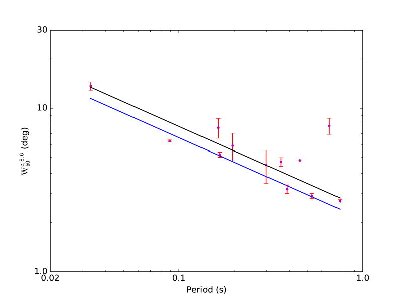
Figure 5: Observed core-component half-power widths at 8.6 GHz plotted against pulse period. Two lower-bound relations are shown, that from Rankin (1990) derived from 1.0 GHz observations (black line), and that for the 8.6 GHz data (blue line).

References

- Abdo et al. (2010) Abdo, A. A., Ajello, M., Antolini, E., et al. 2010, ApJ, 720, 26
- Alurkar et al. (1986) Alurkar, S. K., Bobra, A. D., & Slee, O. B. 1986, Austral. J. Physics, 39, 433
- Basu et al. (2016) Basu, R., Rożko, K., Lewandowski, W., Kijak, J., & Dembska, M. 2016, MNRAS, 458, 2509
- Beskin et al. (1988) Beskin, V. S., Gurevich, A. V., & Istomin, Y. N. 1988, Ap&SS, 146, 205
- Biggs et al. (1988) Biggs, J. D., Lyne, A. G., Hamilton, P. A., McCulloch, P. M., & Manchester, R. N. 1988, MNRAS, 235, 255
- Bilous et al. (2016) Bilous, A. V., Kondratiev, V. I., Kramer, M., et al. 2016, A&A, 591, A134
- Brook et al. (2014) Brook, P. R., Karastergiou, A., Buchner, S., et al. 2014, ApJ, 780, L31
- Cairns et al. (2004) Cairns, I. H., Johnston, S., & Das, P. 2004, MNRAS, 353, 270
- Chen & Wang (2014) Chen, J. L., & Wang, H. G. 2014, ApJS, 215, 11
- Cordes (1978) Cordes, J. M. 1978, ApJ, 222, 1006
- Dai et al. (2015) Dai, S., Hobbs, G., Manchester, R. N., et al. 2015, MNRAS, 449, 3223
- Espinoza et al. (2011) Espinoza, C. M., Lyne, A. G., Stappers, B. W., & Kramer, M. 2011, MNRAS, 414, 1679
- Gould & Lyne (1998) Gould, D. M., & Lyne, A. G. 1998, MNRAS, 301, 235
- Hankins (1971) Hankins, T. H. 1971, ApJ, 169, 487
- Hankins & Fowler (1986) Hankins, T. H., & Fowler, L. A. 1986, ApJ, 304, 256
- Hankins & Rankin (2010) Hankins, T. H., & Rankin, J. M. 2010, AJ, 139, 168
- Hankins & Rickett (1986) Hankins, T. H., & Rickett, B. J. 1986, ApJ, 311, 684
- Hobbs et al. (2004) Hobbs, G., Lyne, A. G., Kramer, M., Martin, C. E., & Jordan, C. 2004, MNRAS, 353, 1311
- Hobbs et al. (2004) Hobbs, G., Faulkner, A., Stairs, I. H., et al. 2004, MNRAS, 352, 1439
- Hotan et al. (2004) Hotan, A. W., van Straten, W., & Manchester, R. N. 2004, PASA, 21, 302
- Johnston (1990) Johnston, S. 1990, PhD thesis, The University of Manchester
- Johnston et al. (2008) Johnston, S., Karastergiou, A., Mitra, D., & Gupta, Y. 2008, MNRAS, 388, 261
- Johnston et al. (2006) Johnston, S., Karastergiou, A., & Willett, K. 2006, MNRAS, 369, 1916
- Johnston & Romani (2002) Johnston, S., & Romani, R. 2002, MNRAS, 332, 109
- Johnston et al. (1993) Johnston, S., Lorimer, D. R., Harrison, P. A., et al. 1993, Nature, 361, 613
- Karastergiou & Johnston (2004) Karastergiou, A., & Johnston, S. 2004, MNRAS, 352, 689
- Karastergiou & Johnston (2006) —. 2006, MNRAS, 365, 353
- Karastergiou et al. (2011) Karastergiou, A., Roberts, S. J., Johnston, S., et al. 2011, MNRAS, 415, 251
- Keith et al. (2011) Keith, M. J., Johnston, S., Levin, L., & Bailes, M. 2011, MNRAS, 416, 346
- Keith et al. (2013) Keith, M. J., Shannon, R. M., & Johnston, S. 2013, MNRAS, 432, 3080
- Kijak et al. (1998) Kijak, J., Kramer, M., Wielebinski, R., & Jessner, A. 1998, A&AS, 127, 153
- Kramer et al. (1997a) Kramer, M., Jessner, A., Doroshenko, O., & Wielebinski, R. 1997a, ApJ, 489, 364
- Kramer et al. (1994) Kramer, M., Wielebinski, R., Jessner, A., Gil, J. A., & Seiradakis, J. H. 1994, A&AS, 107, 515
- Kramer et al. (1997b) Kramer, M., Xilouris, K. M., Jessner, A., et al. 1997b, A&A, 322, 846
- Krishnakumar et al. (2015) Krishnakumar, M. A., Mitra, D., Naidu, A., Joshi, B. C., & Manoharan, P. K. 2015, ApJ, 804, 23
- Large et al. (1968) Large, M. I., Vaughan, A. E., & Wielebinski, R. 1968, Nature, 220, 753
- Lorimer et al. (1995) Lorimer, D. R., Yates, J. A., Lyne, A. G., & Gould, D. M. 1995, MNRAS, 273, 411
- Lyne & Manchester (1988) Lyne, A. G., & Manchester, R. N. 1988, MNRAS, 234, 477
- Malofeev et al. (1994) Malofeev, V. M., Gil, J. A., Jessner, A., et al. 1994, A&A, 285, 201
- Manchester (1971) Manchester, R. N. 1971, ApJS, 23, 283
- Manchester et al. (1980) Manchester, R. N., Hamilton, P. A., & McCulloch, P. M. 1980, MNRAS, 192, 153
- Manchester et al. (2005) Manchester, R. N., Hobbs, G. B., Teoh, A., & Hobbs, M. 2005, AJ, 129, 1993
- Manchester & Taylor (1977) Manchester, R. N., & Taylor, J. H. 1977, Pulsars (San Francisco: Freeman)
- Maron et al. (2000) Maron, O., Kijak, J., Kramer, M., & Wielebinski, R. 2000, A&AS, 147, 195
- Maron et al. (2004) Maron, O., Kijak, J., & Wielebinski, R. 2004, A&A, 413, L19
- Maron et al. (2013) Maron, O., Serylak, M., Kijak, J., et al. 2013, A&A, 555, A28
- McLaughlin & Rankin (2004) McLaughlin, M. A., & Rankin, J. M. 2004, MNRAS, 351, 808
- Mitra & Rankin (2002) Mitra, D., & Rankin, J. M. 2002, ApJ, 322
- Moffett & Hankins (1999) Moffett, D. A., & Hankins, T. H. 1999, ApJ, 522, 1046
- Morris et al. (1981) Morris, D., Graham, D. A., Seiber, W., Bartel, N., & Thomasson, P. 1981, A&AS, 46, 421
- Navarro et al. (1997) Navarro, J., Manchester, R. N., Sandhu, J. S., Kulkarni, S. R., & Bailes, M. 1997, ApJ, 486, 1019
- Pilia et al. (2016) Pilia, M., Hessels, J. W. T., Stappers, B. W., et al. 2016, A&A, 586, A92
- Pilkington et al. (1968) Pilkington, J. D. H., Hewish, A., Bell, S. J., & Cole, T. W. 1968, Nature, 218, 126
- Qiao & Lin (1998) Qiao, G. J., & Lin, W. P. 1998, A&A, 333, 172
- Qiao et al. (2001) Qiao, G. J., Liu, J. F., Zhang, B., & Han, J. L. 2001, A&A, 377, 964
- Qiao et al. (1995) Qiao, G. J., Manchester, R. N., Lyne, A. G., & Gould, D. M. 1995, MNRAS, 274, 572
- Rankin (1983) Rankin, J. M. 1983, ApJ, 274, 333
- Rankin (1990) —. 1990, ApJ, 352, 247
- Rankin (1992) Rankin, J. M. 1992, in IAU Colloq. 128: Magnetospheric Structure and Emission Mechanics of Radio Pulsars, 133
- Rankin (1993) —. 1993, ApJ, 405, 285
- Ravi et al. (2010) Ravi, V., Manchester, R. N., & Hobbs, G. 2010, ApJ, 716, L85
- Ruderman & Sutherland (1975) Ruderman, M. A., & Sutherland, P. G. 1975, ApJ, 196, 51
- Seiradakis et al. (1995) Seiradakis, J. H., Gil, J. A., Graham, D. A., et al. 1995, A&AS, 111, 205
- Sieber (1973) Sieber, W. 1973, A&A, 28, 237
- Sieber et al. (1975) Sieber, W., Reinecke, R., & Wielebinski, R. 1975, A&A, 38, 169
- Slee et al. (1987) Slee, O. B., Bobra, A. D., & Alurkar, S. K. 1987, Aust. J. Phys., 40, 557
- Srostlik & Rankin (2005) Srostlik, Z., & Rankin, J. M. 2005, MNRAS, 362, 1121
- Stairs et al. (1999) Stairs, I. H., Thorsett, S. E., & Camilo, F. 1999, ApJS, 123, 627
- Thorsett (1991) Thorsett, S. E. 1991, ApJ, 377, 263
- Tsai et al. (2016) Tsai, Jr., ., Simonetti, J. H., Akukwe, B., et al. 2016, AJ, 151, 28
- Turtle & Vaughan (1968) Turtle, A. J., & Vaughan, A. E. 1968, Nature, 219, 689
- Vitarmo & Jauho (1973) Vitarmo, J., & Jauho, P. 1973, ApJ, 182, 935
- von Hoensbroech (1999) von Hoensbroech, A. 1999, PhD thesis, University of Bonn
- von Hoensbroech & Xilouris (1997) von Hoensbroech, A., & Xilouris, K. M. 1997, A&AS, 126, 121
- Wang et al. (2015) Wang, J. Q., Zhao, R. B., Yu, L. F., et al. 2015, Acta Astronomica Sinica, 56, 278
- Wang et al. (2001) Wang, N., Manchester, R. N., Zhang, J., et al. 2001, MNRAS, 328, 855
- Weisberg et al. (1999) Weisberg, J. M., Cordes, J. M., Lundgren, S. C., et al. 1999, ApJS, 121, 171
- Weltevrede et al. (2007) Weltevrede, P., Wright, G. A. E., & Stappers, B. W. 2007, A&A, 467, 1163
- Weltevrede et al. (2006) Weltevrede, P., Wright, G. A. E., Stappers, B. W., & Rankin, J. M. 2006, A&A, 459, 597
- Weltevrede et al. (2010) Weltevrede, P., Abdo, A. A., Ackermann, M., et al. 2010, ApJ, 708, 1426
- Wu et al. (1998) Wu, X., Gao, X., Rankin, J. M., Xu, W., & Malofeev, V. M. 1998, AJ, 116, 1984
- Yan et al. (2011) Yan, W. M., Manchester, R. N., van Straten, W., et al. 2011, MNRAS, 414, 2087
- Yan et al. (2015) Yan, Z., Shen, Z.-Q., Wu, X.-J., et al. 2015, ApJ, 814, 5