Scalable Full Flow with Learned Binary Descriptors

Abstract

We propose a method for large displacement optical flow in which local matching costs are learned by a convolutional neural network (CNN) and a smoothness prior is imposed by a conditional random field (CRF). We tackle the computation- and memory-intensive operations on the 4D cost volume by a min-projection which reduces memory complexity from quadratic to linear and binary descriptors for efficient matching. This enables evaluation of the cost on the fly and allows to perform learning and CRF inference on high resolution images without ever storing the 4D cost volume. To address the problem of learning binary descriptors we propose a new hybrid learning scheme. In contrast to current state of the art approaches for learning binary CNNs we can compute the exact non-zero gradient within our model. We compare several methods for training binary descriptors and show results on public available benchmarks.

1 Introduction

Optical flow can be seen as an instance of the dense image matching problem, where the goal is to find for each pixel its corresponding match in the other image. One fundamental question in the dense matching problem is how to choose good descriptors or features. Data mining with convolutional neural networks (CNNs) has recently shown excellent results for learning task-specific image features, outperforming previous methods based on hand-crafted descriptors. One of the major difficulties in learning features for optical flow is the high dimensionality of the cost function: Whereas in stereo, the full cost function can be represented as a 3D volume, the matching cost in optical flow is a 4D volume. Especially at high image resolutions, operations on the flow matching cost are expensive both in terms of memory requirements and computation time.

Our method avoids explicit storage of the full cost volume, both in the learning phase and during inference. This is achieved by a splitting (or min-projection) of the 4D cost into two quasi-independent 3D volumes, corresponding to the $u$ and $v$ component of the flow. We then formulate CNN learning and CRF inference in this reduced setting. This achieves a space complexity linear in the size of the search range, similar to recent stereo methods, which is a significant reduction compared to the quadratic complexity of the full 4D cost function.

Nevertheless, we still have to compute all entries of the 4D cost. This computational bottleneck can be optimized by using binary descriptors, which give a theoretical speed-up factor of $32$. In practice, even larger speed-up factors are attained, since binary descriptors need less memory bandwidth and also yield a better cache efficiency. Consequently, we aim to incorporate a binarization step into the learning. We propose a novel hybrid learning scheme, where we circumvent the problem of hard nonlinearities having zero gradient. We show that our hybrid learning performs almost as well as a network without hard nonlinearities, and much better than the previous state of the art in learning binary CNNs.

2 Related Work

In the past hand-crafted descriptors like SIFT, NCC, FAST etc. have been used extensively with very good results, but recently CNN-based approaches [23, 13] marked a paradigm shift in the field of image matching. To date all top performing methods in the major stereo benchmarks rely heavily on features learned by CNNs. For optical flow, many recent works still use engineered features [5, 1], presumably due to the difficulties the high dimensional optical flow cost function poses for learning. Only very recently we see a shift towards CNNs for learning descriptors [9, 10, 22]. Our work is most related to [22], who construct the full 4D cost volume and run an adapted version of SGM on it. They perform learning and cost volume optimization on $\tfrac{1}{3}$ of the original resolution and compress the cost function in order to cope with the high memory consumption. Our method is memory-efficient thanks to the dimensionality-reduction by the min-projection, and we outperform the reported runtime of [22] by a factor of $10$.

Full flow with CRF [5] is a related inference method using TRW-S [12] with efficient distance transform  [8]. Its iterations have quadratic time and space complexity. In practice, this takes 20GB of memory, and 10-30 sec. per iteration with a parallel CPU implementation. We use the decomposed model [19] with a better memory complexity and a faster parallel inference scheme based on [18].

Hand-crafted Binary Descriptors like Census have been shown to work well in a number of applications, including image matching for stereo and flow  [14, 15, 20, 4]. However, direct learning of binary descriptors is a difficult task, since the hard thresholding function, $\operatorname{sign}(x)$, has gradient zero almost everywhere. In the context of Binary CNNs there are several approaches to train networks with binary activations [2] and even binary weights [7, 16]. This is known to give a considerable compression and speed-up at the price of a tolerable loss of accuracy. To circumvent the problem of $\operatorname{sign}(x)$ having zero gradient a.e., surrogate gradients are used. The simplest method, called straight-through estimator [2] is to assume the derivative of $\operatorname{sign}(x)$ is 1, i.e., simply omit the $\operatorname{sign}$ function in the gradient computation. This approach can be considered as the state of the art, as it gives best results in [2, 7, 16]. We show that in the context of learning binary descriptors for the purpose of matching, alternative strategies are possible which give better results.

3 Method

We define two models for optical flow: a local model, known as Winner-Takes-All (WTA) and a joint model, which uses CRF inference. Both models use CNN descriptors, learned in § 3.1.1. The joint model has only few extra parameters that are fit separately and the inference is solved with a parallel method, see § 3.2. For CNN learning, we optimize the performance of the local model. While learning by optimizing the performance of the joint model is possible [11], the resulting procedures are significantly more difficult.

We assume color images $I^{1},I^{2}\ :\ \Omega\to\mathbb{R}^{3}$, where $\Omega=\{1,\dots H\}\times\{1,\dots W\}$ is a set of pixels. Let $\mathcal{W}=\mathcal{S}\times\mathcal{S}$ be a window of discrete 2D displacements, with $\mathcal{S}=\{-D/2,-D/2+1,\ldots,D/2-1\}$ given by the search window size $D$, an even number. The flow $x\ :\ \Omega\to\mathcal{W}$ associates a displacement to each pixel $i\in\Omega$ so that the displaced position of $i$ is given by $i+x_{i}\in\mathbb{Z}^{2}$. For convenience, we denote by $x=(u,v)$, where $u$ and $v$ are mappings $\Omega\to\mathcal{S}$, the components of the flow in horizontal and vertical directions, respectively. The per-pixel descriptors $\phi(I;\theta)\ :\ \Omega\to\mathbb{R}^{m}$ are computed by a CNN with parameters $\theta$. Let $\phi^{1},\phi^{2}$ be descriptors of images $I^{1}$, $I^{2}$, respectively. The local matching cost for a pixel $i\in\Omega$ and displacement $x_{i}\in\mathcal{W}$ is given by

$$c_{i}(x_{i})=\begin{cases}d(\phi^{1}_{i},\phi^{2}_{i+x_{i}})&{\rm if}\ i+x_{i}\in\Omega,\\ c_{\rm outside}&{\rm otherwise},\end{cases}$$ (1)

where $d\ :\ \mathbb{R}^{m}\times\mathbb{R}^{m}\to\mathbb{R}$ is a distance function in $\mathbb{R}^{m}$. “Distance” is used in a loose sense here, we will consider the negative scalar product $d(\phi^{1},\phi^{2})=-\langle\phi^{1},\phi^{2}\rangle$. We call

$$\hat{x}_{i}\in\arg\min_{x_{i}\in\mathcal{W}}c_{i}(x_{i})$$ (2)

the local optical flow model, which finds independently for each pixel $i$ a displacement $x_{i}$ that optimizes the local matching cost. The joint optical flow model finds the full flow field $x$ optimizing the coupled CRF energy cost:

$$\hat{x}\in\arg\min_{u,v\colon\Omega\to\mathcal{S}}\Big{[}\sum_{i\in\Omega}c_{i}(u_{i},v_{i})+\sum_{i\sim j}w_{ij}(\rho(u_{i}-u_{j})+\rho(v_{i}-v_{j}))\Big{]},$$ (3)

where $i\sim j$ denotes a 4-connected pixel neighborhood, $w_{ij}$ are contrast-sensitive weights, given by $w_{ij}=\exp(-\frac{\alpha}{3}\sum_{c\in\{R,G,B\}}|I^{1}_{i,c}-I^{1}_{j,c}|)$ and $\rho\colon\mathbb{R}\to\mathbb{R}$ is a robust penalty function shown in Fig. 2(a).

3.1 Learning Descriptors

A common difficulty of models (2) and (3) is that they need to process the 4D cost (1), which involves computing distances in $\mathbb{R}^{m}$ per entry. Storing such cost volume takes $\mathcal{O}(|\Omega|D^{2})$ space and evaluating it $\mathcal{O}(|\Omega|D^{2}m)$ time. We can reduce space complexity to $\mathcal{O}(|\Omega|D)$ by avoiding explicit storage of the 4D cost function. This facilitates memory-efficient end-to-end training on high resolution images, without a patch sampling step [22, 13]. Towards this end we write the local optical flow model (2) in the following way

$$\hat{u}_{i} \in\arg\min_{u_{i}}c^{\textsc{u}}_{i}(u_{i}),\ \ \mbox{where}\ \ \ c^{\textsc{u}}_{i}(u_{i})=\min_{v_{i}}c_{i}(u_{i},v_{i});$$ (4a)

$$\hat{v}_{i} \in\arg\min_{v_{i}}c^{\textsc{v}}_{i}(v_{i}),\ \ \mbox{where}\ \ \ c^{\textsc{v}}_{i}(v_{i})=\min_{u_{i}}c_{i}(u_{i},v_{i}).$$ (4b)

The inner step in (4a) and (4b), called min-projection, minimizes out one component of the flow vector. This can be interpreted as a decoupling of the full 4D flow problem into two simpler quasi-independent 3D problems on the reduced cost volumes $c^{\textsc{u}},c^{\textsc{v}}$. Assuming the minimizer of (2) is unique, (4a) and (4b) find the same solution as the original problem (2). Using this representation, CNN learning can be implemented within existing frameworks. We point out that this approach has the same space complexity as recent methods for learning stereo matching, since we only need to store the 3D cost volumes $c^{\textsc{u}}$ and $c^{\textsc{v}}$. As an illustrative example consider an image with size $1024\times 436$ and a search range of 256. In this setting the full 4D cost function takes roughly $108$ GB whereas our splitting consumes only $0.8$ GB.

3.1.1 Network

Fig. 1 shows the network diagram of the local flow model  Eq. 2. The structure is similar to the recent methods proposed for learning stereo matching [13, 23, 6, 11]. It is a siamese network consisting of two convolutional branches with shared parameters, followed by a correlation layer.

Figure 1: Network architecture: A number of convolutional layers with shared parameters computes feature vectors $\phi^{1},\phi^{2}$ for every pixel. These feature vectors are cross-fed into a correlation layer, that computes local matching costs in $u$ and $v$ direction by minimizing out the other direction. The result are two quasi-independent cost volumes for the $u$ and $v$ component of the flow.

The filter size of the convolutions is $3\times 3$ for the first layer and $2\times 2$ for all other layers. The $\tanh$ nonlinearity keeps feature values in a defined range, which works well with the scalar product as distance function. We do not use striding or pooling. The last convolutional layer uses 64 filter channels, all other layers have 96 channels. This fixes the dimensionality of the distance space to $m=64$.

Loss Given the groundtruth flow field $(u^{*},v^{*})$, we pose the learning objective as follows: we define a probabilistic softmax model of the local prediction $u_{i}$ (resp. $v_{i}$) as $p(u_{i})\propto\exp(-c_{i}^{\textsc{u}}(u_{i}))$, then we consider a naive model $p(u,v)=\prod_{i}p(u_{i})p(v_{i})$ and apply the maximum likelihood criterion. The negative log likelihood is given by

$$L(u,v)=-\sum_{i\in\Omega}\big{[}\log p(u_{i}^{*})+\log p(v_{i}^{*})\big{]}.$$ (5)

This is equivalent to cross-entropy loss with the target distribution concentrated at the single point $(u_{i}^{*},v_{i}^{*})$ for each $i$. Variants of the cross-entropy loss, where the target distribution is spread around the ground truth point $(u_{i}^{*},v_{i}^{*})$ are also used in the literature [13] and can be easily incorporated.

3.1.2 Learning Quantized Descriptors

The computational bottleneck in scheme (4) is computing the min-projections, with time complexity $\mathcal{O}(|\Omega|D^{2}m)$. This operation arises during the learning as well as in the CRF inference step, where it corresponds to the message exchange in the dual decomposition. It is therefore desirable to accelerate this step. We achieve a significant speed-up by quantizing the descriptors and evaluating the Hamming distance of binary descriptors.

Let us define the quantization: we call $\bar{\phi}=\operatorname{sign}(\phi)$ the quantized descriptor field. The distance between quantized descriptors is given by $d(\bar{\phi}^{1},\bar{\phi}^{2})=-\langle\bar{\phi}^{1},\bar{\phi}^{2}\rangle=2\mathcal{H}(\bar{\phi}^{1},\bar{\phi}^{2})-m$, equivalent to the Hamming distance $\mathcal{H}(\cdot,\cdot)$ up to a scaling and an offset. Let the quantized cost function be denoted $\bar{c}_{i}(x_{i})$, defined similar to (1). We can then compute quantized min-projections $\bar{c}^{\textsc{u}}$, $\bar{c}^{\textsc{v}}$.

However, learning model (2) with quantized descriptors is difficult due to the gradient of the sign function being zero almost everywhere. We introduce a new technique specific to the matching problem and compare it to the baseline method that uses the straight-through estimator of the gradient [2]. Consider the following variants of the model (4a)

$$\hat{u}_{i}\in\arg\min_{u_{i}}c_{i}(u_{i},\hat{v}_{i}(u_{i})),\ \ \mbox{where}\ \ \ \hat{v}_{i}(u_{i})\in\arg\min_{v_{i}}\bar{c}_{i}(u_{i},v_{i});$$ (FQ)

$$\hat{u}_{i}\in\arg\min_{u_{i}}\bar{c}_{i}(u_{i},\hat{v}_{i}(u_{i})),\ \ \mbox{where}\ \ \ \hat{v}_{i}(u_{i})\in\arg\min_{v_{i}}\bar{c}_{i}(u_{i},v_{i}).$$ (QQ)

The respective variants of (4b) are symmetric. The second letter in the naming scheme indicates whether the inner problem, i.e., the min-projection step, is performed on (Q)uantized or (F)ull cost, whereas the first letter refers to the outer problem on the smaller 3D cost volume. The initial model (4a) is thus also denoted as FF model. While models FF and QQ correspond, up to non-uniqueness of solutions, to the joint minimum in $(u_{i},v_{i})$ of the cost $c$ and $\bar{c}$ respectively, the model FQ is a mixed one. This hybrid model is interesting because minimization in $v_{i}$ can be computed efficiently on the binarized cost with Hamming distance, and the minimization in $u_{i}$ has a non-zero gradient in $c^{\textsc{u}}$. We thus consider the model FQ as an efficient variant of the local optical flow model (2). In addition, it is a good learning proxy for the model QQ: Let $\hat{u}_{i}=\arg\min_{u_{i}}c_{i}(u_{i},\hat{v}_{i}(u_{i}))$ be a minimizer of the outer problem FQ. Then the derivative of FQ is defined by the indicator of the pair $(\hat{u}_{i},\hat{v}_{i}(u_{i}))$. This is the same as the derivative of FF, except that $\hat{v}_{i}(u_{i})$ is computed differently. Learning the model QQ involves a hard quantization step, and we apply the straight-through estimator to compute a gradient. Note that the exact gradient for the model FQ can be computed at approximately the same reduced computational cost as the straight-through gradient in the model QQ.

3.2 CRF

The baseline model, which we call product model, has $|\Omega|$ variables $x_{i}$ with the state space $S\times S$. It has been observed in [8] that max-product message passing in the CRF (3) can be computed in time $\mathcal{O}(D^{2})$ per variable for separable interactions using a fast distance transform. However, storing the messages for a 4-connected graph requires $\mathcal{O}(|\Omega|D^{2})$ memory. Although such an approach was shown feasible even for large displacement optical flow [5], we argue that a more compact decomposed model [19] gives comparable results and is much faster in practice. The decomposed model is constructed by observing that the regularization in (3) is separable over $u$ and $v$. Then the energy (3) can be represented as a CRF with $2|\Omega|$ variables $u_{i},v_{i}$ with the following pairwise terms: The in-plane term $w_{ij}\rho(u_{i}-u_{j})$ and the cross-plane term $c(u_{i},v_{i})$, forming the graph shown in Fig. 2(b). In this formulation there are no unary terms, since costs $c_{i}$ are interpreted as pairwise terms. The resulting linear programming (LP) dual is more economical, because it has only $\mathcal{O}(|\Omega|D)$ variables. The message passing for edges inside planes and across planes has complexity $\mathcal{O}(|\Omega|D)$ and $O(|\Omega|D^{2})$, respectively.

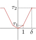
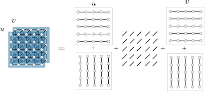
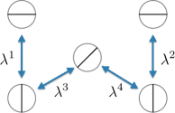
(a)	(b)	(c)

Figure 2: Building blocks of the CRF. (a) Robust pairwise function $\rho$. (b) Decomposition of the pairwise CRF into 5 subproblems. (c) Lagrange multipliers in the dual corresponding to equality constraints between the subproblems. They act as offsets of unary costs between subproblems, increasing on one side of the arrow and decreasing on the other.

We apply the parallel inference method [18] to the dual of the decomposed model [19] (see Fig. 2(b)). Although different dual decompositions reach different objective values in a fixed number of iterations, it is known that all decompositions with trees covering the graph are equivalent in the optimal value [21]. The decomposition in Fig. 2(b) is into horizontal and vertical chains in each of the $u$- and $v$- planes plus a subproblem containing all cross-layer edges. We introduce Lagrange multipliers $\lambda=(\lambda^{k}\in\mathbb{R}^{\Omega\times\mathcal{S}}\mid k=1,2,3,4)$ enforcing equality constraints between the subproblems as shown in Fig. 2(c). The Lagrange multipliers $\lambda^{k}$ are identified with modular functions $\lambda^{k}\colon\mathcal{S}^{\Omega}\to\mathbb{R}\colon u\mapsto\sum_{i}\lambda^{k}_{i}(u_{i})$. Let us also introduce shorthands for the sum of pairwise terms over horizontal chains $f^{\rm h}\colon\mathcal{S}^{\Omega}\to\mathbb{R}\colon u\mapsto\sum_{ij\in\mathcal{E}^{\rm h}}w_{ij}\rho(u_{i}-u_{j})$, and a symmetric definition $f^{\rm v}$ for the sum over the vertical chains. The lower bound $\Psi(\lambda)$ corresponding to the decomposition in Fig. 2(c) is given by:

$$\Psi(\lambda)=\ \Psi^{1}(\lambda)+\Psi^{2}(\lambda)+\Psi^{3}(\lambda),\mbox{\ where}$$ (6a)

$$\Psi^{1}(\lambda)=\min\limits_{u}\big{[}(\lambda^{1}+\lambda^{3})(u)+f^{\rm h}(u)\big{]}+\min\limits_{u}\big{[}-\lambda^{1}(u)+f^{\rm v}(u)\big{]};$$ (6b)

$$\Psi^{2}(\lambda)=\min\limits_{v}\big{[}(\lambda^{2}+\lambda^{4})(v)+f^{\rm h}(v)\big{]}+\min\limits_{v}\big{[}-\lambda^{2}(v)+f^{\rm v}(v)\big{]};$$ (6c)

$$\Psi^{3}(\lambda)=\sum_{i}\min_{u_{i},v_{i}}\big{[}c_{i}(u_{i},v_{i})-\lambda_{i}^{3}(u_{i})-\lambda_{i}^{4}(v_{i})\big{]}.$$ (6d)

Our Lagrangian dual to (3) is to maximize $\Psi(\lambda)$ in $\lambda$, which enforces consistency between minimizers of the subproblems. The general theory [21] applies, in particular, when the minimizers of all subproblems are consistent they form a global minimizer. In (6b), there is a sum of horizontal and vertical chain subproblems in the $u$-plane. When $\lambda^{3}$ is fixed, $\Psi^{1}(\lambda)$ is the lower bound corresponding to the relaxation of the energy in $u$ with the unary terms given by $\lambda^{3}$. It can be interpreted as a stereo-like problem with 1D labels $u$. Similarly, $\Psi^{2}(\lambda)$ is a lower bound for the $v$-plane with unary terms $\lambda^{4}$. Subproblem $\Psi^{3}(\lambda)$ is simple, it contains both variables $u,v$ but the minimization decouples over individual pairs $(u_{i},v_{i})$. It connects the two stereo-like problems through the 4D cost volume $c$.

Updating messages inside planes can be done at a different rate than across planes. The optimal rate for fast convergence depends on the time complexity of the message updates. [19] reported an optimal rate of updating in-plane messages 5 times as often using the TRW-S solver [12]. The decomposition (6a) facilitates this kind of strategy and allows to use the implementation [18] designed for stereo-like problems. We therefore use the dual solver [18], denoted Dual Minorize-Maximize (DMM) to perform in-plane updates. When applied to the problem of maximizing $\Psi^{1}(\lambda)$ in $\lambda^{1}$, it has the following properties: a) the bound $\Psi^{1}(\lambda)$ does not decrease and b) it computes a modular minorant $s$ such that $s(u)\leq\lambda^{3}(u)+f^{\rm h}(u)+f^{\rm v}(u)$ for all $u$ and $\Psi^{1}(\lambda)=\sum_{i}\min_{u_{i}}s_{i}(u_{i})$. The modular minorant $s$ is an excess of costs, called slacks, which can be subtracted from $\lambda^{3}$ while keeping $\Psi^{1}(\lambda)$ non-negative. The associated update of the $u$-plane can be denoted as

$$(\lambda^{1},s) :={\rm DMM}(\lambda^{1},\lambda^{3},f^{\rm h},f^{\rm v}),$$ (7a)

$$\lambda^{3} :=\lambda^{3}-s.$$ (7b)

The slack $s$ is then passed to the $v$ plane by the following updates, i.e., message passing $u\rightarrow v$:

$$\lambda_{i}^{4}(v_{i}):=\lambda_{i}^{4}(v_{i})+\min_{u_{i}}\big{[}c_{i}(u_{i},v_{i})-\lambda_{i}^{3}(u_{i})\big{]}.$$ (8)

The minimization (8) has time complexity $\mathcal{O}(|\Omega|D^{2})$, assuming the 4D costs $c_{i}$ are available in memory. As discussed above, we can compute the costs $c_{i}$ efficiently on the fly and avoid $\mathcal{O}(|\Omega|D^{2})$ storage. The update $v\rightarrow u$ is symmetric to (7a):

$$\lambda_{i}^{3}(u_{i}):=\lambda_{i}^{3}(u_{i})+\min_{v_{i}}\big{[}c_{i}(u_{i},v_{i})-\lambda_{i}^{4}(v_{i})\big{]}.$$ (9)

The complete method is summarized in Algorithm 1. It starts from collecting the slacks in the $u$-plane. When initialized with $\lambda=0$, the update (9) simplifies to $\lambda^{3}_{i}(u_{i})=\min_{v_{u}}c_{i}(u_{i},v_{i})$, i.e., it is exactly matching to the min-projection $c^{\textsc{u}}$ (4). The problem solved with DMM in Algorithm 1 in the first iteration is a stereo-like problem with cost $c^{\textsc{u}}$. The dual solution redistributes the costs and determines which values of $u$ are worse than others, and expresses this cost offset in $\lambda^{3}$ as specified in (7a). The optimization of the $v$-plane then continues with some information of good solutions for $u$ propagated via the cost offsets using (8).

Input: Cost volume $c$;

Output: Dual point $\lambda$ optimizing $\Psi(\lambda)$;

1 Initialize $\lambda:=0$;

2 for $t=1,\dots,\mbox{{it\_outer}}$ do

3       Perform the following updates:

4       $v\rightarrow u$: pass slacks to $u$-plane by (9), changes $\lambda^{3}$;

5       $u$-plane: DMM with it_inner iterations for $u$-plane (7a), changes $\lambda^{1}$, $\lambda^{3}$ ;

6       $u\rightarrow v$: pass slacks to $v$-plane by (8), changes $\lambda^{4}$;

7       $v$-plane: DMM with it_inner iterations for $v$-plane, changes $\lambda^{2}$, $\lambda^{4}$;

8      

Algorithm 1 Flow CRF Optimization

4 Evaluation

We compare different variants of our own model on the Sintel optical flow dataset [3]. In total the benchmark consists of 1064 training images and 564 test images. For CNN learning we use a subset of $20\%$ of the training images, sampled evenly from all available scenes. For evaluation, we use a subset of $40\%$ of the training images.

Comparison of our models To investigate the performance of our model, we conduct the following experiments: First, we investigate the influence of the size of the CNN, and second we investigate the effect of quantizing the learned features. Additionally, we evaluate both the WTA solution (2), and the CRF model (3). To assess the effect of quantization, we evaluate the local flow model a) as it was trained, and b) QQ, i.e., with quantized descriptors both in the min-projection step as well as in the outer problem on $c^{\textsc{u}},c^{\textsc{v}}$ respectively. In CRF inference the updates (8) and (9) amount to solving a min-projection step with additional cost offsets. F and Q indicate how this min-projection step is computed. CRF parameters are fixed at $\alpha=8.5,~{}\eqref{joint-problem},\ \tau_{1}=0.25,\ \tau_{2}=25$ (Fig. 2) for all experiments and we run 8 inner and 5 outer iterations. Table 1 summarizes the comparison of different variants of our model.

Table 1: Comparison of our models on a representative validation set at scale $\tfrac{1}{2}$. We present the end-point-error (EPE) for non-occluded (noc) and all pixels on Sintel clean.

		Local Flow Model (WTA)		CRF
Train	#Layers	as trained	QQ	F	Q
		noc (all)	noc (all)	noc (all)	noc (all)
FF	5	5.25 (10.38)	10.45 (15.67)	1.58 (4.48)	1.64 (4.87)
	7	4.72 (10.04)	9.43 (14.93)	1.53 (4.32)	1.61 (4.70)
	9	–	–	–	–
FQ	5	6.15 (11.36)	11.43 (16.78)	–	1.63 (4.62)
	7	5.62 (10.98)	10.15 (15.70)	–	1.65 (4.62)
	9	5.62 (11.13)	9.87 (15.52)	–	1.64 (4.69)
QQ	5	same as QQ	9.63 (14.80)	–	1.72 (4.91)
	7	same as QQ	9.75 (15.23)	–	1.66 (4.78)
	9	same as QQ	9.72 (15.31)	–	1.72 (4.85)

We see that the WTA solution of model FQ performs similarly to FF, while being much faster to train and evaluate. In particular, model FQ performs better than QQ, which was trained with the straight through estimator of the gradient. If we switch to QQ for evaluation, we see a drop in performance for models FF and FQ. This is to be expected, because we now evaluate costs differently than during training. Interestingly, our joint model yields similar performance regardless whether we use F or Q for computing the costs.

4.0.1 Runtime

The main reason for quantizing the descriptors is speed. In CRF inference, we need to compute the min-projection on the 4D cost function twice per outer iteration, see Alg. 1. We show an exact breakdown of the timings for $D=128$ on full resolution images in Table 3, computed on a Intel i7 6700K and a Nvidia Titan X.

Table 2: Timings of the building blocks (seconds).

Method	Feature Extraction	WTA	Full Model
FF	0.04 – 0.08	4.25	24.8
FQ	0.04 – 0.08	1.82	-
QQ	0.04 – 0.08	0.07	3.2
[22] ($\tfrac{1}{3}$ res.)	0.02	0.06	3.4
QQ ($\tfrac{1}{3}$ res.)	0.004 – 0.008	0.007	0.32

Table 3: Comparison on the Sintel clean test set.

Method	noc	all
EpicFlow [17]	1.360	4.115
FullFlow [5]	1.296	3.601
FlowFields [1]	1.056	3.748
DCFlow [22]	1.103	3.537
Ours QQ	2.470	8.972

The column WTA refers to computing the solution of the local model on the cost volumes $c^{\textsc{u}},c^{\textsc{v}}$, see Eq. 4. Full model is the CRF inference, see § 3.2. We see that we can reach a significant speed-up by using binary descriptors and Hamming distance for computing intensive calculations. For comparison, we also report the runtime of [22], who, at the time of writing, report the fastest execution time on Sintel. We point out that our CRF inference on full resolution images takes about the same time as their method, which constructs and optimizes the cost function at $\tfrac{1}{3}$ resolution.

Test performance We compare our method on the Sintel clean images. In contrast to the other methods we do not use a sophisticated post-processing pipeline, because the main focus of this work is to show that learning and inference on high resolution images is feasible. Therefore we cannot compete with the highly tuned methods. Fig. 3 shows that we are able to recover fine details, but since we do not employ a forward-backward check and local planar inpainting we make large errors in occluded regions.

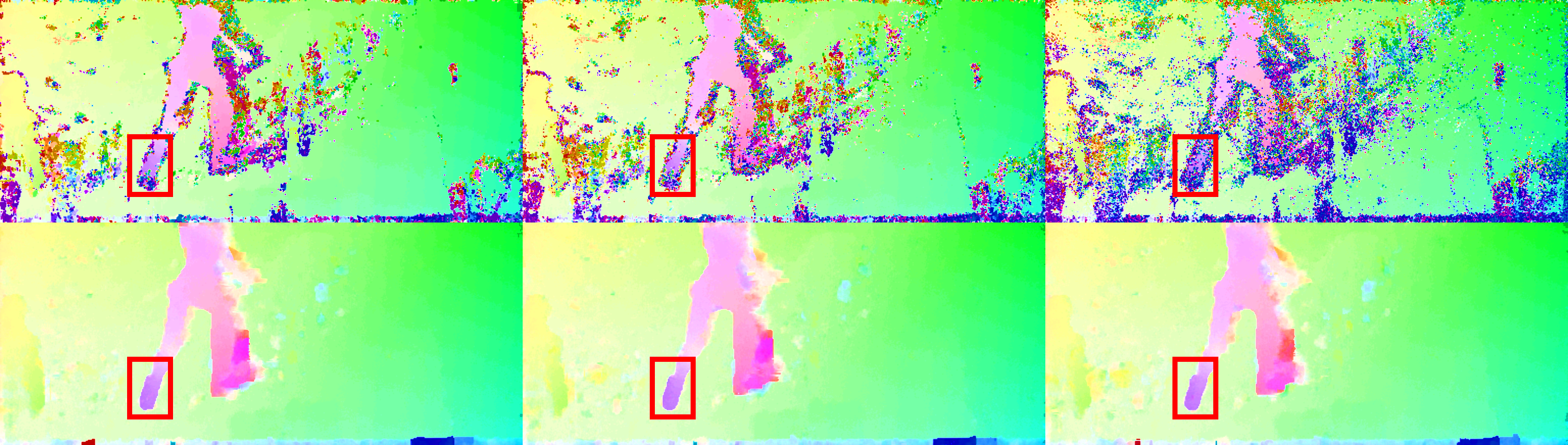
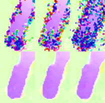
Figure 3: Sample output of our method. Left figure, top row shows the WTA solution of a 7-layer network for FF, FQ, QQ training. The bottom row shows results of the same network with CRF inference. The right part shows the highlighted region enlarged.

5 Conclusion

We showed that both learning and CRF inference of the optical flow cost function on high resolution images is tractable. We circumvent the excessive memory requirements of the full 4D cost volume by a min-projection. This reduces the space complexity from quadratic to linear in the search range. To efficiently compute the cost function, we learn binary descriptors with a new hybrid learning scheme, that outperforms the previous state-of-the-art straight-through estimator of the gradient.

Acknowledgements

We acknowledge grant support from Toyota Motor Europe HS, the ERC starting grant ”HOMOVIS” No. 640156 and the research initiative Intelligent Vision Austria with funding from the AIT and the Austrian Federal Ministry of Science, Research and Economy HRSM programme (BGBl. II Nr. 292/2012)

References

- [1] Bailer, C., Taetz, B., Stricker, D.: Flow fields: Dense correspondence fields for highly accurate large displacement optical flow estimation. In: International Conference on Computer Vision (ICCV) (2015)
- [2] Bengio, Y., Léonard, N., Courville, A.C.: Estimating or propagating gradients through stochastic neurons for conditional computation. CoRR abs/1308.3432 (2013), http://arxiv.org/abs/1308.3432
- [3] Butler, D.J., Wulff, J., Stanley, G.B., Black, M.J.: A naturalistic open source movie for optical flow evaluation. In: European Conference on Computer Vision (ECCV) (2012)
- [4] Calonder, M., Lepetit, V., Strecha, C., Fua, P.: Brief: Binary robust independent elementary features. In: European Conference on Computer Vision (ECCV) (2010)
- [5] Chen, Q., Koltun, V.: Full flow: Optical flow estimation by global optimization over regular grids. In: Conference on Computer Vision and Pattern Recognition (CVPR) (2016)
- [6] Chen, Z., Sun, X., Wang, L., Yu, Y., Huang, C.: A deep visual correspondence embedding model for stereo matching costs. In: International Conference on Computer Vision (ICCV) (2015)
- [7] Courbariaux, M., Bengio, Y.: Binarynet: Training deep neural networks with weights and activations constrained to +1 or -1. CoRR abs/1602.02830 (2016), http://arxiv.org/abs/1602.02830
- [8] Felzenszwalb, P.F., Huttenlocher, D.P.: Efficient belief propagation for early vision. International Journal of Computer Vision 70(1), 41–54 (2006)
- [9] Gadot, D., Wolf, L.: Patchbatch: A batch augmented loss for optical flow. In: Conference on Computer Vision and Pattern Recognition, (CVPR) (2016)
- [10] Güney, F., Geiger, A.: Deep discrete flow. In: Asian Conference on Computer Vision (ACCV) (2016)
- [11] Knöbelreiter, P., Reinbacher, C., Shekhovtsov, A., Pock, T.: End-to-end training of hybrid CNN-CRF models for stereo. In: Conference on Computer Vision and Pattern Recognition, (CVPR) (2017), http://arxiv.org/abs/1611.10229
- [12] Kolmogorov, V.: Convergent tree-reweighted message passing for energy minimization. Transactions on Pattern Analysis and Machine Intelligence 28(10) (october 2006)
- [13] Luo, W., Schwing, A., Urtasun, R.: Efficient deep learning for stereo matching. In: International Conference on Computer Vision and Pattern Recognition (ICCV) (2016)
- [14] Ranftl, R., Bredies, K., Pock, T.: Non-local total generalized variation for optical flow estimation. In: European Conference on Computer Vision (ECCV) (2014)
- [15] Ranftl, R., Gehrig, S., Pock, T., Bischof, H.: Pushing the limits of stereo using variational stereo estimation. In: IEEE Intelligent Vehicles Symposium (IV) (2012)
- [16] Rastegari, M., Ordonez, V., Redmon, J., Farhadi, A.: Xnor-net: Imagenet classification using binary convolutional neural networks. In: European Conference on Computer Vision (ECCV) (2016)
- [17] Revaud, J., Weinzaepfel, P., Harchaoui, Z., Schmid, C.: EpicFlow: Edge-Preserving Interpolation of Correspondences for Optical Flow. In: Computer Vision and Pattern Recognition (CVPR) (2015)
- [18] Shekhovtsov, A., Reinbacher, C., Graber, G., Pock, T.: Solving Dense Image Matching in Real-Time using Discrete-Continuous Optimization. ArXiv e-prints (Jan 2016)
- [19] Shekhovtsov, A., Kovtun, I., Hlaváč, V.: Efficient MRF deformation model for non-rigid image matching. CVIU 112 (2008)
- [20] Trzcinski, T., Christoudias, M., Fua, P., Lepetit, V.: Boosting binary keypoint descriptors. In: Conference on Computer Vision and Pattern Recognition (CVPR) (2013)
- [21] Wainwright, M., Jaakkola, T., Willsky, A.: MAP estimation via agreement on (hyper)trees: Message-passing and linear-programming approaches. IT 51(11) (November 2005)
- [22] Xu, J., Ranftl, R., Koltun, V.: Accurate Optical Flow via Direct Cost Volume Processing. In: Conference on Computer Vision and Pattern Recognition (CVPR) (2017)
- [23] Žbontar, J., LeCun, Y.: Computing the stereo matching cost with a convolutional neural network. In: Conference on Computer Vision and Pattern Recognition (CVPR) (2015)