The core - cusp problem: a matter of perspective
Abstract
The existence of two kinematically and chemically distinct stellar subpopulations in the Sculptor and Fornax dwarf galaxies offers the opportunity to constrain the density profile of their matter haloes by measuring the mass contained within the well-separated half-light radii of the two metallicity subpopulations. Walker and Peñarrubia have used this approach to argue that data for these galaxies are consistent with constant-density ‘cores’ in their inner regions and rule out ‘cuspy’ Navarro–Frenk–White (NFW) profiles with high statistical significance, particularly in the case of Sculptor. We test the validity of these claims using dwarf galaxies in the APOSTLE (A Project Of Simulating The Local Environment) cold dark matter cosmological hydrodynamic simulations of analogues of the Local Group. These galaxies all have NFW dark matter density profiles and a subset of them develop two distinct metallicity subpopulations reminiscent of Sculptor and Fornax. We apply a method analogous to that of Walker and Peñarrubia to a sample of 50 simulated dwarfs and find that this procedure often leads to a statistically significant detection of a core in the profile when in reality there is a cusp. Although multiple factors contribute to these failures, the main cause is a violation of the assumption of spherical symmetry upon which the mass estimators are based. The stellar populations of the simulated dwarfs tend to be significantly elongated and, in several cases, the two metallicity populations have different asphericity and are misaligned. As a result, a wide range of slopes of the density profile are inferred depending on the angle from which the galaxy is viewed.
keywords:
galaxies: kinematics and dynamics –galaxies: dwarf – galaxies: formation – dark matter1 Introduction
One of the fundamental predictions of the cold dark matter () model of cosmogony is that dark matter assembles into haloes that, in the absence of baryon effects, develop steeply rising inner radial density profiles, or cusps. This important result was obtained from -body simulations which showed that the density distribution of a dark matter halo of any mass is well fit by a Navarro–Frenk–White profile (NFW; Navarro et al., 1996, 1997) independently of initial conditions and cosmological parameters.
The inner slope of the NFW profile follows . In contrast, measurements of galaxy rotation curves and dynamical models of dwarf spheroidal galaxies are often claimed to require shallower density profile slopes that are consistent with a constant-density core at the centre, (e.g. Moore, 1994; Flores & Primack, 1994; Battaglia et al., 2008; Walker & Peñarrubia, 2011; Amorisco & Evans, 2012; Agnello & Evans, 2012; Adams et al., 2014; Oh et al., 2015). This disagreement between observations and simulations has become known as the core-cusp problem.
In order to resolve this discrepancy, a number of mechanisms involving baryons, which could transform cusps into cores, have been proposed. For example, cores may be created when baryons, after slowly condensing at the centre of a halo, are suddenly expelled by supernova feedback, either in a single event (Navarro et al., 1996; Read & Gilmore, 2005) or through repeated episodes of star formation (Pontzen & Governato, 2012; Brooks & Zolotov, 2014). Alternatively, energy could be transferred to the outer halo by clumps infalling due to dynamical friction (Sánchez-Salcedo et al., 2006; Mashchenko et al., 2008; Cole et al., 2011; El-Zant et al., 2001; Del Popolo & Kroupa, 2009), or through resonant effects induced by a central stellar bar (Weinberg & Katz, 2002).
Dwarf spheroidal galaxies are promising objects to test ideas about the inner structure of dark matter haloes. These galaxies are strongly dark-matter dominated (Pryor & Kormendy, 1990) and, although they are faint, some are sufficiently close-by that their stellar populations can be resolved. Much effort has therefore been invested in trying to infer their halo profiles. A large body of work is concerned with field galaxies with measurable H i velocity fields; many such studies claim robust detections of central cores (e.g. Oh et al., 2011; Kuzio de Naray et al., 2006; Adams et al., 2014). However, a recent study (Oman et al., 2017), based on the same APOSTLE (A Project Of Simulating The Local Environment) simulations that we will analyse here, has revealed the presence of systematic effects in even the most detailed analyses of spatially resolved kinematics, casting doubt on claims that cores are present in those galaxies. Similar conclusions were reached by Pineda et al. (2017).
The kinematics of resolved stars in nearby galaxies offer an alternative to the kinematics of H i gas as a probe of the density structure of haloes. The detection of cores in several dwarf satellites of the Milky Way has been claimed on the basis of simple Jeans analyses (e.g. Gilmore et al., 2007), but the more general analysis by Strigari et al. (2010) has shown that current data are, in fact, unable to distinguish between cores and cusps in the Milky Way satellites. Some satellites of the Milky Way and Andromeda exhibit metallicity gradients: they have a centrally concentrated metal-rich population and a more extended, and kinematically hotter metal-poor population (Tolstoy et al., 2004; Battaglia et al., 2008, 2011). The origin of these systems is unknown but major mergers (Benítez-Llambay et al., 2016), reaccretion of gas (Tolstoy et al., 2004; Battaglia et al., 2006) or effects due to reionization (Kawata et al., 2006) have been proposed as possible origins of metallicity gradients.
The presence of two kinematically and spatially distinct metallicity components can be used to set constraints on the inner density profile of the common halo in which they move. Battaglia et al. (2008) identified a metal-rich () and a metal-poor () population in the Sculptor dwarf spheroidal and, using Jeans modelling, found that a wide range of profiles are consistent with the data, from a pseudo-isothermal sphere ( at the centre) to an NFW profile. Amorisco & Evans (2012) pointed out that some of those models are unphysical and, fitting the Sculptor data to a particular phase-space distribution function, found that while a profile with a core is preferred by their fits, an NFW profile is also allowed by the data. Using more general phase-space distribution functions, Strigari et al. (2014) also showed that the two metallicity subpopulations in Sculptor are consistent with an NFW profile. A similar conclusion, using Schwarzschild modelling, was reached by Breddels et al. (2013) who found that a core profile is also allowed, while a cusp in Sculptor was found to be favoured by an analysis based on the fourth-order virial theorem by Richardson & Fairbairn (2014).
Walker & Peñarrubia (2011) took this idea further and developed a statistical methodology to distinguish the two metallicity subpopulations in Sculptor and Fornax. Making use of the interesting result of Wolf et al. (2010) and Walker et al. (2009) that the mass of a spherical stellar system in equilibrium can be robustly estimated at the half-mass radius of the system, they developed the method discussed in this paper and concluded that both Sculptor and Fornax have central cores, with Sculptor, in particular, ruling out an NFW profile at high statistical significance. Their method is based on estimating the total mass contained within the half-light radii of the metal-rich and metal-poor subpopulations, thus constraining the slope of the dark matter density profile. Wolf et al. (2010) and Walker et al. (2009) have argued that the mass within a characteristic radius of a collisionless spherical system in dynamical equilibrium is well constrained by the velocity dispersion and average radial distribution of a population of star tracers, for a variety of stellar density and constant velocity anisotropy profiles.
Specifically, Wolf et al. (2010) showed that the mass is best constrained at radius, , where the logarithmic slope of the stellar number density, , which is close to the deprojected half-light radius (, where is the projected half-light radius) for a range of stellar distributions. Their estimator is:
| (1) |
where is the luminosity-averaged line-of-sight velocity dispersion. Similarly, Walker et al. (2009) propose:
| (2) |
Walker & Peñarrubia (2011) used a likelihood method to separate samples of stars in Sculptor and Fornax into two metallicity subcomponents and applied these mass estimators to each of them. For an object with mass density the enclosed mass is . One can then define the asymptotic logarithmic mass slope as:
| (3) |
For an NFW profile the asymptotic inner slope is = 1, so , while for a core with = 0, . In the case of a galaxy with two segregated subpopulations, the two half-light radii will be located away from the centre and thus is a measure of the (steeper) density slope further out (Walker & Peñarrubia, 2011). Assuming that the mass is given by the estimators above,
| (4) |
where are the line-of-sight velocity dispersions and are the half-light radii. Walker & Peñarrubia (2011) derived values of for Sculptor and Fornax which exclude an NFW cusp at 99 and 96 per cent confidence levels, respectively, instead favouring a core. They argue that this conclusion is conservative because, if anything, the mass is likely to be overestimated for the central subpopulation.
In a recent paper Campbell et al. (2017) tested the accuracy of the mass estimators by applying them to galaxies in the APOSTLE hydrodynamic cosmological simulations of Local Group analogues (for which the true mass is known; see Section 2). They report little bias in the median mass estimates but a scatter of 25 and 23 per cent for the Walker et al. (2009) and Wolf et al. (2010) estimators respectively, which are much larger than the values inferred by these authors from simulations of spherical systems in dynamical equilibrium. Campbell et al. (2017) find that a major contribution to the scatter comes from deviations from spherical symmetry which are quite common in simulated galaxies. Subsequently, González-Samaniego et al. (2017) have generally confirmed the main conclusions of Campbell et al. (2017) regarding the scatter in the estimator from 12 dwarf galaxy analogues in the FIRE hydrodynamic simulations.
The effect of triaxality on has been investigated by Laporte et al. (2013a), who tagged dark matter particles as stars in the (triaxial) dark matter haloes of the AQUARIUS simulations (Springel et al., 2008). These authors find that an anti-correlation between the measured half-light radius and the projected velocity dispersion acts to keep the mass estimate approximately constant, causing little variation in the derived value of . However, by construction, the dark matter and the stars in their analysis have strongly correlated shapes (Laporte et al., 2013b) which can introduce a systematic effect.
Kowalczyk et al. (2013) carried out idealized -body simulations of the evolution of dwarf spheroidal galaxies in the gravitational potential of a Milky Way-like host. They introduced two spatially segregated disc subpopulations which evolve as the dwarf orbits in the halo of its host. They find that may be over- or underestimated, depending on the line of sight. In particular, observations along the major axis of the dwarf tend to overestimate the mass and . These simulations do not take into account dark matter halo triaxality, hydrodynamics, star formation or feedback processes.
Campbell et al. (2017) focused on the accuracy of the mass estimators applied to the stellar population of the dwarf galaxies in APOSTLE as a whole. Many of these galaxies, however, turn out to have two (or more) distinct metallicity subpopulations, analogous to those in Sculptor or Fornax. This offers the possibility of testing the validity of the conclusions of Walker & Peñarrubia (2011) using realistic dwarf galaxies formed in state-of-the-art cosmological simulations. This is the goal of this paper. In Section 2 we outline the selection of our simulated galaxy sample and perform an analogous analysis to that of Walker & Peñarrubia (2011). In Section 3 we examine in detail a selection of case studies. We summarize our conclusions in Section 4.
2 Simulations and methods
| Volume | [M⊙] | [M⊙] | [M⊙] |
|---|---|---|---|
| AP-1 | 3.5 | 7.0 | 0.4-1.4 |
| AP-4 | 1.7 | 3.5 | 0.2-1.0 |
| AP-6 | 3.7 | 7.5 | 0.4-2.5 |
| AP-10 | 3.6 | 7.2 | 0.4-1.2 |
| AP-11 | 3.5 | 7.1 | 0.4-1.6 |
2.1 APOSTLE simulations
APOSTLE consists of a suite of zoom-in hydrodynamical simulations of analogues of the Local Group environment (Fattahi et al., 2016; Sawala et al., 2016). The regions were selected for resimulation from the 100 Mpc on a side cosmological -body simulation DOVE (Jenkins, 2013). The Milky Way - Andromeda analogues were chosen based on the galaxy pair separations, total mass, relative velocities, recession velocities of the outer Local Group members and consistency with the environment surrounding the Local Group. WMAP-7 cosmological parameters are assumed: density parameters, = 0.272, = 0.0455 and = 0.728; reduced Hubble constant = 0.704; spectral index = 0.967 and power spectrum normalization, = 0.81 (Komatsu et al., 2011). An ionizing background is switched on instantaneously at =11.5.
The regions were resimulated using the eagle code, an improved version of the -body/Smooth Particle Hydrodynamics (SPH) code P-gadget-3 (Crain et al., 2015; Schaye et al., 2015; Springel, 2005), including subgrid prescriptions for supernovae and AGN feedback (Dalla Vecchia & Schaye, 2012; Booth & Schaye, 2009), gas cooling and heating (Wiersma et al., 2009a), reionization, star formation and metal enrichment (Schaye, 2004; Schaye & Dalla Vecchia, 2008; Wiersma et al., 2009b) and black hole formation and mergers (Rosas-Guevara et al., 2015). The Tree-PM scheme of P-gadget-3 is used to compute the gravitational acceleration and the ANARCHY SPH scheme (Dalla Vecchia & Schaye, 2012; Schaller et al., 2015), based on the pressure-entropy formalism of Hopkins (2013), is used to compute hydrodynamical forces.
The APOSTLE suite consists of 12 volumes simulated at low and medium resolution (L2 and L3). Five of these were also resimulated at high resolution (L1). In this work we will only consider galaxies within the high-resolution volumes. The gas, dark matter and stellar particle masses for each of these may be found in Table 1.
2.2 Galaxy sample
Haloes in the simulations are identified using the ‘friends-of-friends’ (FOF) algorithm with linking length of 0.2 times the mean particle separation (Davis et al., 1985). The SUBFIND algorithm is then used to identify gravitationally bound substructures within them (Springel et al., 2001). We define the host and subhalo centres as the centre of their potential (the position of the particle with the most negative potential energy).
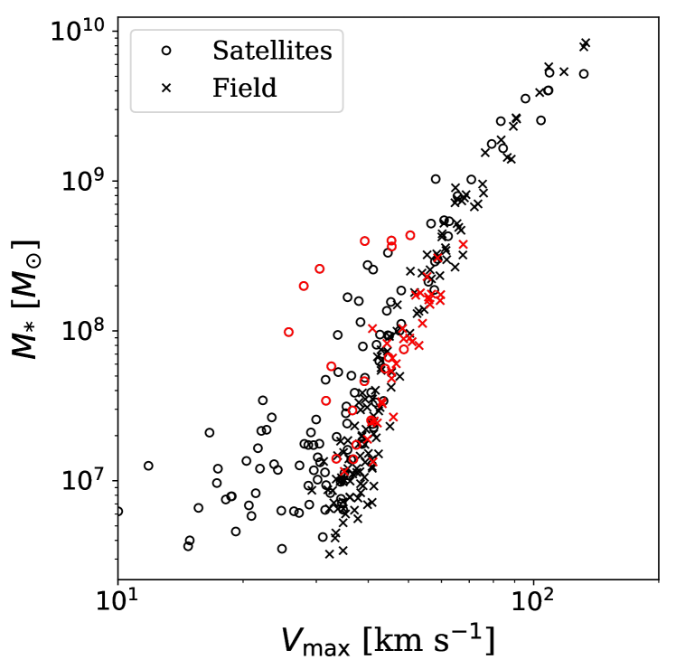
Subhaloes bound to the main halo of a group are defined here as ‘satellites’; other galaxies in the volume are labelled as ‘field’ galaxies. When computing the stellar mass of a subhalo, we include all particles located within 0.15 of the virial radius, , for field galaxies and particles located within the tidal radius111We define the tidal radius of a subhalo as a distance from subhalo centre where the mean enclosed density is equal to that of the host halo up to that distance for satellite galaxies. for satellite galaxies. We limit the sample of satellites and field galaxies to those with a minimum of 1000 stellar particles [corresponding to a stellar mass of the order of ] to ensure reasonable statistics and good resolution within the half-mass222We use the term half-mass radius to refer to the radius enclosing half the stellar mass as measured directly from the simulations. radius. The stellar mass as a function of the maximum circular velocity, , of galaxies in the five high resolution volumes is shown in Fig. 1.
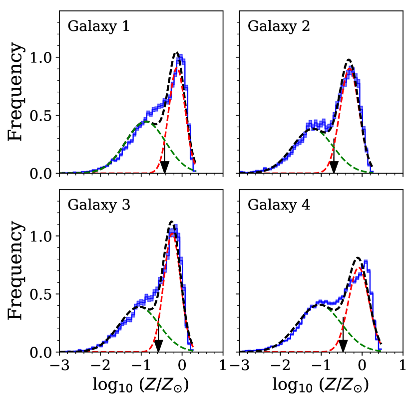
In order to identify particles belonging to each stellar subpopulation, for every individual satellite and field galaxy we model the subcomponents using Gaussian Mixture Modelling (GMM) whereby the total metallicity distribution, , is fitted with a combination of two Gaussian probability density functions333As a measure of metallicity we use , the logarithm of the abundance of elements other than hydrogen and helium. Stellar particles in APOSTLE are spawned probabilistically, with daughter particles inheriting smoothed metal abundances from their parent. For details see Okamoto et al. (2005); Okamoto et al. (2014). (Hastie et al., 2001). Five parameters are fit altogether (, , , , ), with being the relative weight of one of the subpopulations, the mean metallicity and the metallicity dispersion. We then assign each particle to a subpopulation if its probability of being in that subpopulation is . Effectively, the population is rigidly split at the value of metallicity where the two Gaussians cross. The subpopulation with a higher value of is denoted as metal-rich and that with the lower as metal-poor. A sharp cut in metallicity gives rise to some kinematic mixing of the two subpopulations. We have verified that mixing has only a minor effect on the main results of this paper regarding the slope of the halo density profile (see Section A2).
It is important to note, first, that the metallicity distributions of the two subpopulations will not necessarily be Gaussian, but will depend on the specifics of the history of star formation, accretion and mergers. We choose Gaussian probability densities for simplicity. Secondly, cases may exist, where indeed more than two subpopulations are present. These objects would be of great interest for future work due to the possibility of constraining the inner density slope at two or more locations.
In principle, any probability distribution will be better fitted with Gaussian mixtures as the number of fitting parameters is increased. We therefore calculate the Akaike Information Criterion (AIC) corrected for finite sample (Akaike, 1998):
| (5) |
where is the number of fitted parameters, is the number of data points and is the chi-squared fit of our model to the data. We take the histogram errors to be Poisson-distributed. The first and third terms in equation (5) represent the penalty on the number of free parameters in the model such that the difference between the AIC values for alternative models is indicative of the information gained by including extra parameters. We find the AIC for a model with a single Gaussian and a model with a mixture of two Gaussians for each galaxy in our sample. We then remove objects where the AIC for a single Gaussian is smaller than that for a mixture of two, as well as those where both models provide a poor fit. A total of 46 per cent of all galaxies satisfy these criteria. The metallicity histograms and subpopulation models of specific objects that we will discuss in particular detail later are shown in Fig. 2.
A simple split into two metallicity subcomponents does not guarantee that they will be spatially segregated. We remove from our sample the objects for which the separation between the two half-light radii is so small as to inflate artificially, as approaches zero (see Fig. A11). We therefore discard all objects for which the logarithm of the ratio of 3D half-mass radii, 0.06. This condition removes a further 26 per cent of our original sample. For the remaining galaxies, we check that the metal-rich and metal-poor radii are well resolved as judged by the convergence radius defined by Power et al. (2003), at which the collisional relaxation time is approximately equal to the age of the Universe, ensuring that both radii are larger than this value. Overall, of all objects with over 1000 stellar particles in the five high-resolution volumes of APOSTLE, 18 per cent (50 objects) survive our selection criteria. The selected objects are shown in red in Fig. 1; they have stellar masses of the order of 107 - 108 . We find that the fraction of stellar particles assigned to the metal-poor subpopulation ranges between 0.15 and 0.6, consistently with the results of Benítez-Llambay et al. (2016); the metal-rich stellar particles are typically the dominant subcomponent.

2.3 A test of the Walker-Peñarrubia prescription
We now carry out a straightforward test of the accuracy of the logarithmic mass slopes obtained following the Walker & Peñarrubia (2011) prescription. We generate 10 random lines of sight distributed uniformly on the surface of a sphere. For each line of sight, we obtain 1000 bootstrap stellar particle samples for each galaxy, with replacement and, for each sample, we calculate projected half-mass radii, , directly as the projected radius within which half the total stellar mass is contained444According to González-Samaniego et al. (2017) this method of estimating results in the bias of 0.9 in the estimated mass seen in the 12 FIRE simulations. However, using a much larger sample of galaxies in APOSTLE, Campbell et al. (2017) found that the mass estimate is, in fact, unbiased. We choose to calculate the projected half-mass radii as in Campbell et al. (2017).. We then calculate the mass-averaged line-of-sight velocity dispersion as:
| (6) |
where is the mass of each star particle, is the velocity of the particle in projection and is the mean velocity.
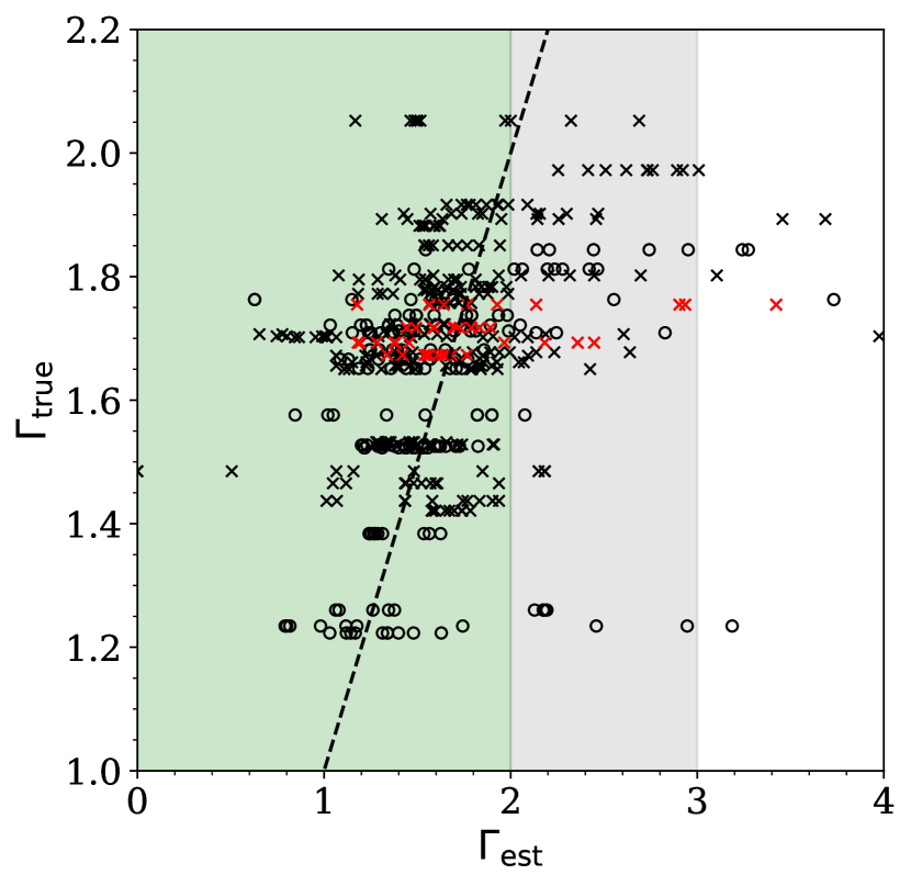
Inserting our measured values of and in the Walker et al. (2009) estimator (equation 2) we obtain the estimated mass within of each subpopulation. For each galaxy, we repeat this calculation for the 1000 bootstrap resamplings and for 10 random directions. In Fig. 3 we plot , the slope of the line joining the logarithm of the actual mass within the true projected 3D half-mass radius of each subpopulation555We take the true projected 3D half-mass radius of an object to be 3/4 of the 3D half-mass radius measured from the simulation., as a function of the median values of , the slope of the line joining the logarithm of the estimated mass within the measured of each subpopulation.
It is clear that the estimated mass slopes tend to be underestimated on average, consistent with findings of Walker & Peñarrubia (2011), and thus the inferred slopes of the density profiles tend to be cuspier than the true values. (Recall that corresponds to an NFW cusp, while corresponds to a core.) The distribution is asymmetric and exhibits large scatter towards higher values of , with some objects reaching . This bias reflects biases in the measurements of and as the galaxy is seen from different observer positions. We now investigate why the measured half-mass radii and velocity dispersions vary with the viewing direction.
2.4 Dynamical properties of the simulated galaxies
Campbell et al. (2017) identified asphericity, rotation and velocity anisotropy as the key properties that can introduce uncertainty in mass measurements based on stellar kinematics. We now quantify these properties for each metallicity subpopulation within each galaxy in our sample and examine the extent to which the properties of the two subpopulations are correlated with each other666As discussed in Section B1, we have checked that the two subpopulations of the galaxies in our sample have a sufficiently large number of stellar particles for the properties of interest to be numerically converged..
2.4.1 Sphericity
Here we define the centre of each stellar subpopulation as its centre of mass. The shape of the system is characterized by the reduced inertia tensor (Bett et al., 2007):
| (7) |
where is the stellar mass of the subpopulation; the mass of star particle ; and are the coordinates of particle from the centre of the galaxy in directions and . The normalization ensures that only the angular distribution is taken into account, so that the shape is not unduly affected by distant particles. The eigenvectors of the inertia tensor correspond to the axes of the fitted ellipsoid and the eigenvalues, to squares of axis lengths. We define the sphericity ; corresponds to a sphere.
The sphericities of the metal-rich and metal-poor subpopulations in our sample are plotted against each other in the left panel of Fig. 4. The two are positively correlated, albeit with significant scatter caused by one of the subpopulations in certain objects being appreciably more spherical than the other. These cases are of particular interest in this study. Also note that the satellites tend to be less aspherical than the field galaxies. This is likely due to the effects of tidal stripping as discussed in detail in the work of Barber et al. (2015).
2.4.2 Rotation
We quantify the degree to which each subpopulation is supported by rotation by computing , the fraction of kinetic energy invested in rotational motion (Sales et al., 2012):
| (8) |
where is the stellar kinetic energy of the subpopulation, the mass of star particle , the component of the specific angular momentum of the particle in the direction of the total angular momentum and the distance of the particle from the angular momentum axis. Objects with are considered to be primarily rotation-dominated, while objects with < 0.5 are considered to be primarily dispersion-dominated.
The values of for subpopulations of galaxies in our sample are shown in the middle panel of Fig. 4. Our selected objects are generally dispersion-dominated and a strong bias exists towards higher in the metal-rich subpopulation compared to the metal-poor. All simulated galaxies considered in this work have 0.5 for the galaxy as a whole.
2.4.3 Velocity anisotropy
The velocity anisotropy is defined as =-/2, where is the radial velocity dispersion and the tangential velocity dispersion including the contributions from azimuthal and polar directions. We construct velocity anisotropy profiles by calculating and for the 32 nearest neighbours of each star particle.
The right panel of Fig. 4 shows the average velocity anisotropy, , for each metallicity subpopulation (the average of local anisotropy of each particle). The majority of the galaxies in our sample tend to have radially biased stellar velocity distributions and the anisotropies are generally correlated in the two metallcity subpopulations. Yet, cases exist where is radially biased for one subpopulation and tangentially biased or isotropic for the other. As we shall see, such discrepancies affect estimates of .
3 The effects of projection: four case studies
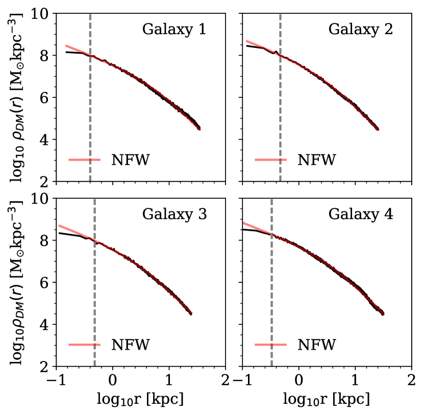
In Fig. 3 we saw that a procedure analogous to that implemented by Walker & Peñarrubia (2011) in their analysis of the kinematics of Sculptor and Fornax dwarfs generally underestimates the logarithmic mass slopes , albeit with a large scatter towards higher values, which would correspond to shallower inner density slopes. We now investigate the factors that affect the accuracy of the procedure. We first examine in detail four illustrative examples and in Section 3.2 we collect the results for our sample of 50 galaxies. We recall that the dark matter density profiles of all the galaxies in our sample are well described by an NFW profile.
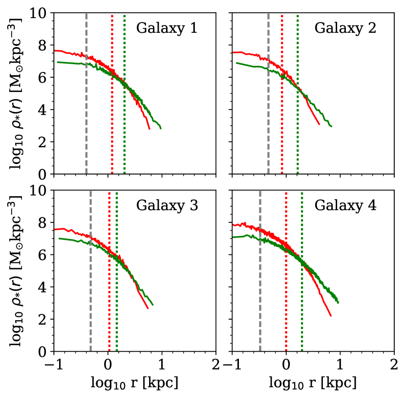
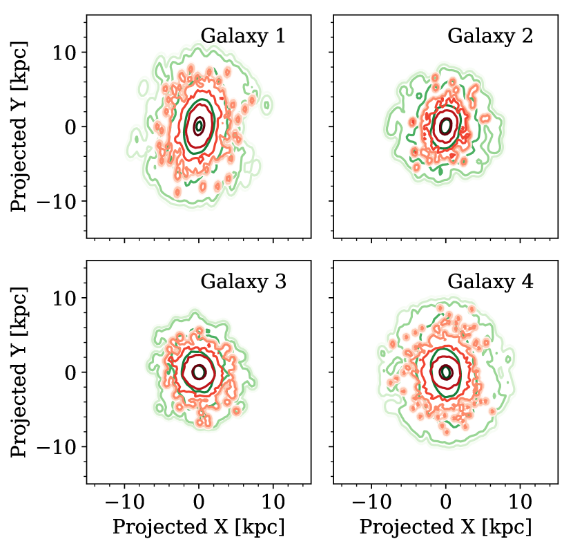
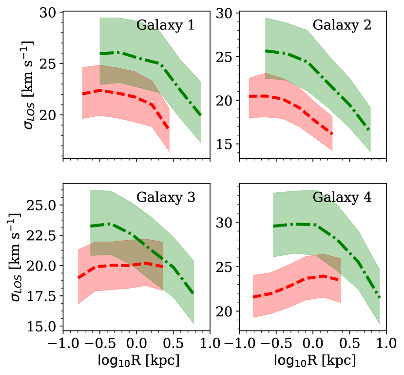
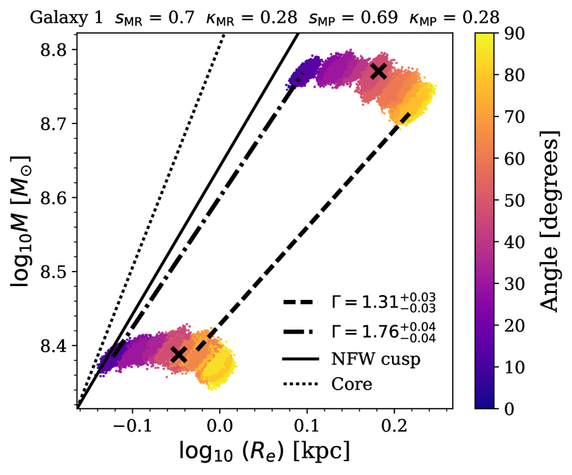
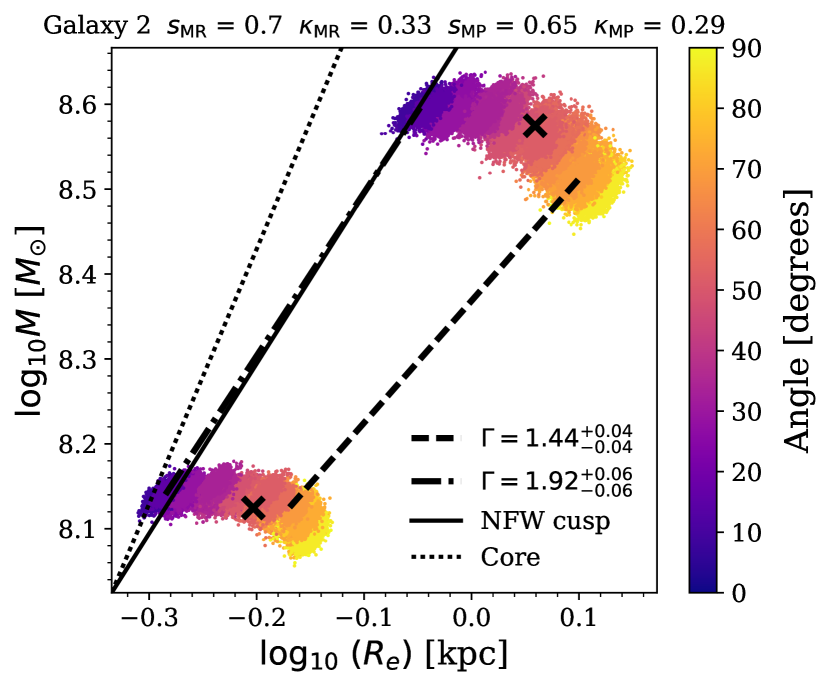
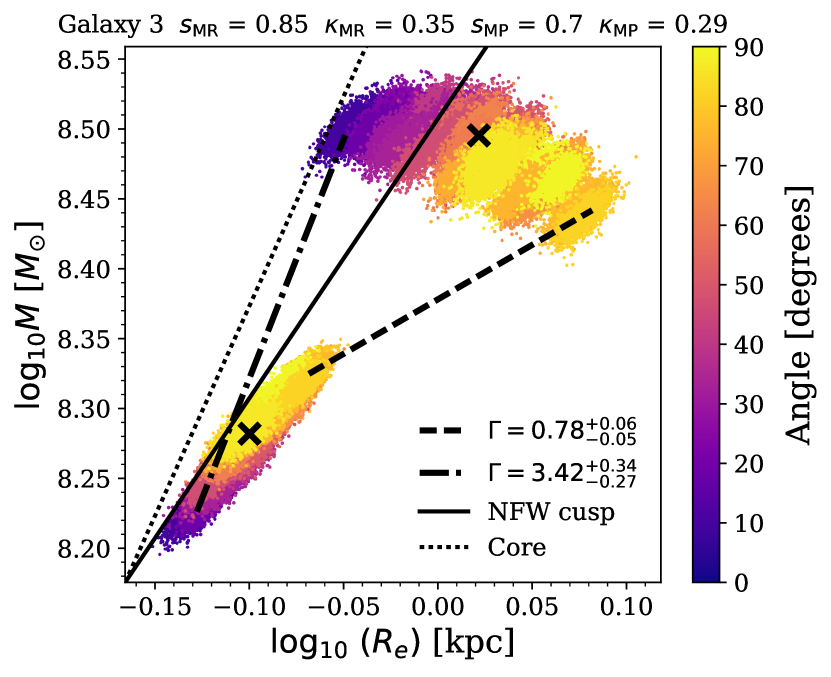
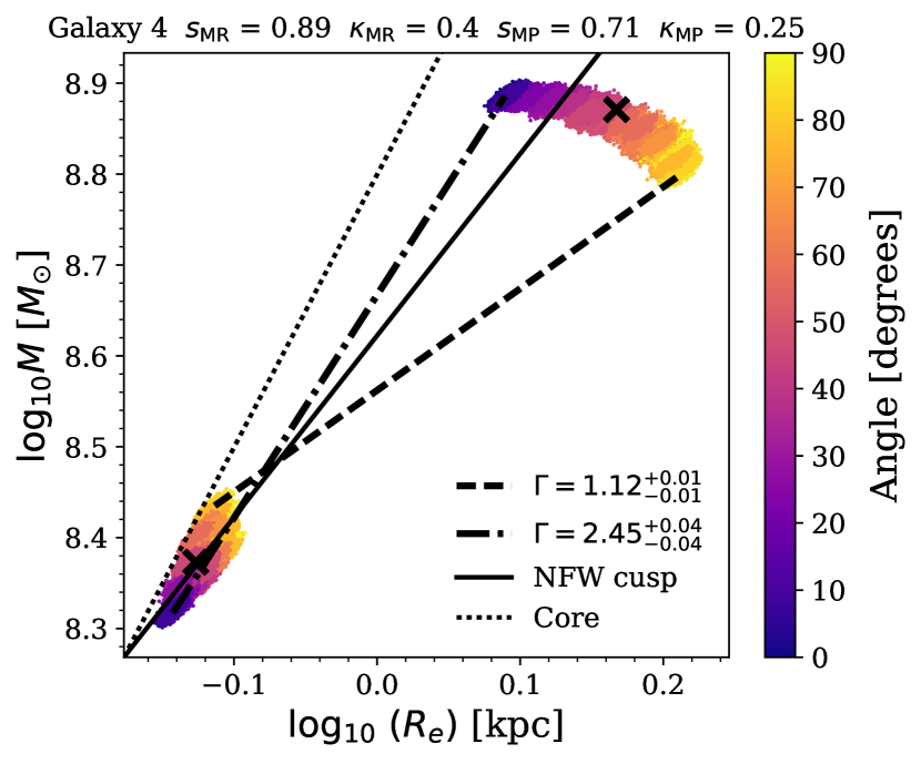
The four examples are highlighted in red in Fig. 3. All four are isolated field galaxies, with no recent major mergers. Their two metallicity subpopulations are well segregated spatially. The line-of-sight velocity dispersion of the metal-poor subpopulation is higher than that of the metal-rich subpopulation (see Fig. 5 for the properties of the four examples). In two cases (Galaxies 1 and 2) the procedure on average recovers an accurate value of the slope, but in the other two (Galaxies 3 and 4) the procedure fails and, instead of a cusp, it often returns a profile with a core.
3.1 The effects of misalignment and anisotropy
We view each galaxy from 100 random directions generated uniformly on the surface of a sphere using the spherical spiral method outlined in González (2009). As in Section 2.3, for each line of sight we generate 1000 bootstrap resamplings (with replacement) of the stars in each galaxy and obtain median values of the quantities of interest. In Fig. 6, which is analogous to fig. 10 of Walker & Peñarrubia (2011), we plot the logarithm of the measured projected half-mass radii of the bootstrap samples for each viewing angle, along with the corresponding logarithm of masses contained within these radii, inferred using the estimator of equation (2). The measurements are coloured according to the angle between the line of sight and the major axis of the metal-poor subpopulation. (The major axes of the two subpopulations will not necessarily be aligned.) The true projected 3D half-mass radius and the enclosed mass of each subpopulation are marked by a cross. The sphericity and value of for each metallicity subpopulation are given in the legend of each panel. For each viewing angle the inferred slope of the cumulative logarithmic mass profile can be obtained by joining points of the same colour in the metal-rich and metal-poor subpopulations. The dashed and dot-dashed lines show the minimum and maximum slopes inferred by this procedure.
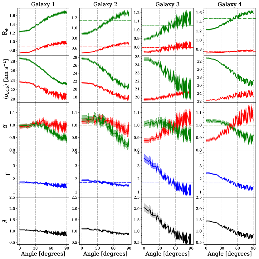
The variation with viewing angle of relevant quantities for each galaxy is plotted in Fig. 7 and is discussed below. In this plot, denotes the ratio, , of the estimated to the true mass, where the true mass includes the dark matter, stellar and gas particles within the projected 3D half-mass radius; is the ratio, , of the estimated to the true slope of the cumulative logarithmic mass profile, where is the slope measured between the measured values of and is the slope between the projected true 3D half-mass radii of the two subpopulations.
Apart from the metal-rich subpopulation of Galaxy 4, which is close to spherical, all other subpopulations in the four examples of Fig. 6 are quite elongated. For the nearly spherical subpopulation, the estimated projected half-mass radius is, not surprisingly, almost independent of viewing angle. The values of the estimated mass show a mild systematic dependence on viewing angle which reflects the weak dependence of the velocity dispersion on the line of sight seen in Fig. 7.
The situation is quite different for the elongated subpopulations. Let us consider, for example, the metal-poor subpopulation of Galaxy 4. Its sphericity is , quite typical for our sample (see Fig. 4). Now the measured values of the projected half-mass radius vary greatly with viewing angle, from 1.2 kpc when the subpopulation is viewed along its major axis to 1.6 kpc when it is viewed along the perpendicular direction. Since the velocity anisotropy is radially biased (see Fig. 4), the measured velocity dispersion varies with viewing angle, from 33 km s-1 when viewed along the major axis to 27 km s-1 when viewed along the perpendicular direction. This decrease in velocity dispersion largely balances the increase in the projected half-mass radius with the result that the estimated mass of the metal-poor population varies little with viewing angle, by only 0.1 dex. Thus, a very similar mass is associated with a relatively large range of projected half-mass radii. The biases in the measured mass are anticorrelated as the viewing angle varies, as shown in the third row of Fig. 7.
As Figs 6 and 7 show, the result is that the inferred slope of the cumulative logarithmic mass profile for Galaxy 4 can take on a wide range of values, from when the galaxy is viewed along the major axis of the metal-poor population to when it is viewed along the perpendicular direction. Thus, for viewing angles between about 0 and 50∘, the mass distribution in this galaxy would, incorrectly, be measured to have a core.
Galaxies 1 and 2 are also quite elongated. However, in these two cases, both subpopulations are aspherical and their major axes are roughly aligned. Now the behaviour we have just seen for the metal-poor subpopulation of Galaxy 4 is reproduced for both subpopulations. The result is that both the projected half-mass radius and the mass contained within it for both subpopulations are incorrectly estimated by roughly the same factors and these biases vary similarly with viewing angle (third row of Fig. 7). Thus, although the masses and radii of both subpopulations are incorrectly estimated, the slopes come out roughly right: these two galaxies are correctly inferred to have cusps.
Galaxy 3 is an intermediate case. Its metal-poor subpopulation has similar sphericity to the metal-poor subpopulation of Galaxy 4 so the measured projected half-mass radius varies by a similar factor. While the inferred mass has greater scatter at a given viewing angle, the overall variation is still only slightly larger than 0.1 dex. The half-mass radius of the metal-rich subpopulation of Galaxy 3 shows some dependence on viewing angle (see Fig. 7). In this case, the systematic variation of the inferred mass is larger and, as seen in Fig. 7, it increases with viewing angle. This is enough to result in a wide range of estimated slopes. Similarly to Galaxy 4, this galaxy would be measured to have a core for viewing angles between about 20 and 50∘ and for even smaller viewing angles it would be measured to have a ‘hole’ in the central region ().
Although the systematic errors in the estimates of the slope of the cumulative logarithmic mass distribution using a procedure analogous to that of Walker & Peñarrubia (2011) result from a complex interplay between projection and kinematic effects, it is clear that a major factor behind them is the significant elongation of the stellar subpopulations, and particularly the misalignment between the major axes of the metal-rich and metal-poor subpopulations seen in a number of cases, including Galaxy 4. This lack of similarity arises naturally in our simulations and is linked to the different formation paths of the two subpopulations (Benítez-Llambay et al., 2016), which we will investigate in a subsequent paper.
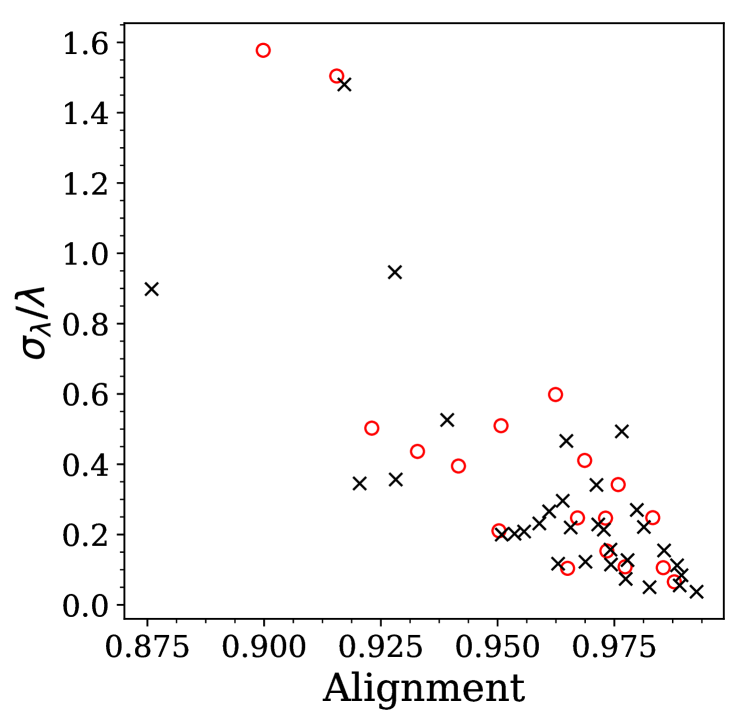
In order to quantify the effect of both the misalignment of the principal axes and the differences in sphericity of the two subpopulations on the scatter in the estimated logarithmic mass slopes, we define the following alignment statistic. We model the two subpopulations as concentric ellipsoids of unit volume, with axis ratios equal to those measured for each subpopulation and an offset angle equal the angle between the major axes of the two subpopulations. We then compute the fraction of volume within the intersection of the two ellipsoids. Subpopulations with similar axis ratios and spatial orientation would therefore have an alignment close to 1. In Fig. 8 we show the relative upper error (the difference between the 84th and 50th percentiles divided by the median value) on the slope accuracy, , as a function of the value of the alignment statistic. It is clear that measurements for galaxies with more misaligned subpopulations tend to return higher values of , corresponding to shallower inner density slopes.
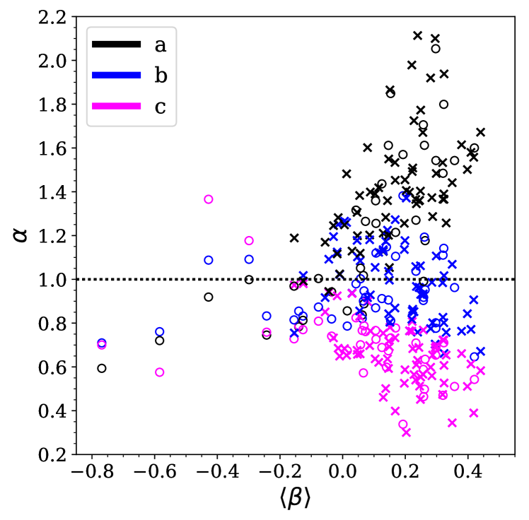
The non-trivial radial variation of the velocity anistropy, , which is generally different for the two metallicity subpopulations (see Fig. 4), also plays a role. This can be seen in Fig. 9, where we plot , the error in the estimate of the mass for each of the two subpopulations in our sample, as a function of the average anisotropy parameter , when each subpopulation is viewed from directions aligned with the three principal axes. For directions along the minor and intermediate axes the values of scatter about , although there is a bias towards , that is for an underestimate of the mass when the subpopulation is viewed along its minor axis. However, when the subpopulation is viewed along its major axis and the velocity anisotropy has a radial bias () , its mass tends to be overestimated [in agreement with the conclusions of Kowalczyk et al. (2013)] and the size of this bias increases systematically with increasing anisotropy. Along this particular viewing angle the velocity dispersion is generally largest. When the velocity distribution is isotropic or tangentially biased, however, the mass is correctly estimated. (This is the reason why the estimate of the mass of the metal-rich subpopulation of Galaxy 3, which has an isotropic velocity distribution, is unbiased.)
3.2 Accuracy of the inferred mass slope for the sample as a whole
In this subsection we present statistical results for our sample of 50 galaxies. This sample was selected according to the specific criteria described in Section 2.2, essentially requiring that there be two well-separated metallicity subpopulations, as judged by the statistic introduced in that section. These criteria need not match in detail those used for real objects. At present there are only a handful of two-metallicity subpopulation galaxies known and those populations have been identified somewhat serendipitously. Nevertheless, our statistical results should be indicative of the frequency with which we might expect the slope of the dark matter density profile to be incorrectly estimated.
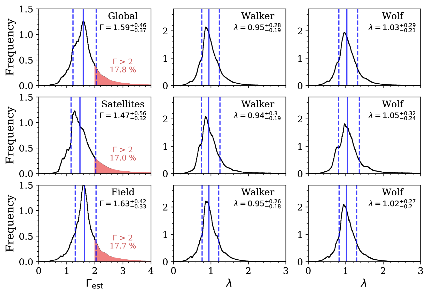
The top panel of Fig. 10 shows the distributions of and for the 1000 bootstrap resamplings of each galaxy in our sample, each viewed from 100 different random directions. (Recall that an NFW profile has as and a profile with a constant-density core has .) The distribution of is asymmetric with mean value = 1.59 and = 0.95 for the Walker et al. (2009) estimator, implying that is underestimated on average by 5 per cent; the true value (corresponding to ) lies within 1 of the mean. Slopes tend to be overestimated by 3 per cent on average using the Wolf et al. (2010) estimator, with = 1.03.
Flatter slopes than NFW, are measured in per cent of cases and (corresponding to a ‘hole’ in the centre) in per cent of cases. In the middle and bottom panels we show equivalent distributions for satellite and field galaxies in our sample. Whilst the satellites generally tend to exhibit cuspier inner slopes ( = 1.47 compared to = 1.63 for field dwarfs), the distribution of the accuracy of the inferred slopes, , is similar to that of the field galaxies. The greater scatter towards higher values of in satellites can be explained by the fact that a greater fraction of satellites than field galaxies in our sample exhibit strong misalignment, as shown in Fig. 8. We have additionally verified that if we identify the true slope with the slope of the line joining the logarithm of true masses within of each subpopulation, the bias and scatter in remain unaffected.
Walker & Peñarrubia (2011), who used the Walker et al. (2009) estimator, found for Sculptor and for Fornax and concluded that these values exclude the NFW profile with significance greater than 99 and 96 per cent respectively. However, according to the distribution of in Fig. 10 for the Walker et al. (2009) and Wolf et al. (2010) estimators derived from our simulations, these values of are only inconsistent with the NFW profile at 93.6 and 88.9 significance for Sculptor and Fornax respectively (where we have taken the 1 lower limit of the original estimates).
4 Discussion and Conclusions
The question of whether or not the dark matter haloes of galaxies have central, constant-density cores is of great interest in cosmology. It is now well established that, in the absence of baryon effects, haloes of all masses develop NFW profiles (Navarro et al., 1996, 1997) which have a central cusp. An incontrovertible measurement of a core would therefore have important implications: it would either signal the impact of exotic baryonic effects (Navarro et al., 1996; Pontzen & Governato, 2012) or of exotic types of particles such as self-interacting dark matter (Spergel & Steinhardt, 2000). Unfortunately measuring dark matter profiles in the innermost regions of haloes, encompassing only at most a few per cent of the halo mass, is difficult.
In this work we have tested the Walker & Peñarrubia (2011) procedure for inferring the slope of the inner dark matter halo profile in galaxies with two metallicity subpopulations using galaxies from the APOSTLE cosmological simulations. These follow not only the evolution of dark matter, but also the evolution of gas, and incorporate subgrid prescriptions to model the processes thought to be at play in galaxy formation. The initial conditions correspond to a cold dark matter universe but are conditioned to form an analogue of the Local Group at the final time. Thus, this is the first test of the Walker & Peñarrubia (2011) procedure in fully realistic simulations which produce dwarf galaxies ab initio. These are not guaranteed to satisfy the key assumptions underlying the Wolf et al. (2010) and Walker et al. (2009) mass estimators: sphericity and dynamical equilibrium, and indeed, many of our simulated galaxies violate them to varying degrees.
Gratifyingly, our simulations produce dwarf galaxies with two identifiable metallicity subpopulations reminiscent of Sculptor and Fornax. Out of 286 model galaxies resolved with more than 1000 stellar particles we identify 50 dwarfs with dual metallicity subpopulations, according to the criteria discussed in Section 2.2. Their kinematical properties are summarized in Fig. 4. The subpopulations tend to be significantly aspherical and often develop different asphericities: per cent of galaxies in our sample have metal-rich and metal-poor subpopulations differing in sphericity by over 10 per cent and, in many cases, the orientation of their major axes differs as well. The metal-rich subpopulations tend to show more rotation than the metal-poor ones and the velocity anisotropy of the subpopulations can also differ substantially. These differences occur both in satellites and in field dwarfs. The lack of similarity arises naturally in our simulations and is linked to the different formation paths of the two subpopulations (which we will investigate in a subsequent paper).
Our main result is that the method introduced by Battaglia et al. (2008) and extended by Walker & Peñarrubia (2011), based on comparing the masses interior to the half-mass radii of the metal-rich and metal-poor subpopulations, can often lead to an incorrect inference of the slope of the inner profile of the galaxies’ dark matter haloes. All the haloes in our simulations have cuspy NFW profiles, yet 17.8 per cent of the galaxies in our sample would be inferred to have flatter, core-like profiles. Multiple factors play a role in these failures but the main culprit is misalignment of the two elongated metallicity subpopulations (which generally have radially varying velocity anisotropy). This results in a wide range of inferred slopes for the mass distribution depending on the viewing angle. Four specific examples illustrating cases when the slope is correctly or incorrectly inferred have been shown.
The study of Walker & Peñarrubia (2011) is sometimes regarded as one of the more convincing arguments for the presence of cores in the dark matter haloes of dwarf galaxies (Amorisco & Evans, 2012). However, their proposed method of measuring cumulative logarithmic mass profile slopes relies heavily on the assumption that the properties of the two metallicity subpopulations are correlated, such that any bias in the application of the mass estimator would cancel when obtaining the slope. This assumption fails in a number of our simulated galaxies where not only the elongation and orientation, but also the orbital anisotropy differs for the two subpopulations. Of course it remains to be seen whether the properties of the two metallicity subpopulations in Sculptor and Fornax are correlated or not, but this is not currently feasible. The availability of proper motion data for individual stars within these galaxies would allow us to somewhat take away the dependence of the accuracy of the mass estimator on the angle of view, although, for an instrument like Gaia, the measurement uncertainties for a galaxy as distant as Sculptor is expected to be comparable to the velocities themselves (Gaia Collaboration et al., 2016; Jin et al., 2015). Given the sensitivity of the inferred slope to the viewing angle that we have demonstrated in this work, we concur with Kowalczyk et al. (2013) that a large statistical sample of randomly oriented galaxies is highly desirable. But for any particular observation, knowledge of the sphericity and velocity anisotropy of both subpopulations and their orientation with respect to one another and to the observer is required before any definitive conclusion can be reached regarding the slope of the galaxy’s inner dark matter halo.
Acknowledgments
We thank the anonymous referee for useful comments that helped us improve the final version of this work. We are also grateful for helpful discussions with Marius Cautun, Aaron Ludlow, Matthieu Schaller, Louis Strigari and Alis Deason. This work was supported by the Science and Technology Facilities Council grants ST/L00075X/1 and ST/P000451/1. AG acknowledges an STFC studentship funded by STFC grant ST/N50404X/1. This work used the DiRAC Data Centric system at Durham University, operated by the Institute for Computational Cosmology on behalf of the STFC DiRAC HPC Facility (www.dirac.ac.uk). This equipment was funded by BIS National E-infrastructure capital grant ST/K00042X/1, STFC capital grant ST/H008519/1, STFC DiRAC Operations grant ST/K003267/1 and Durham University. DiRAC is part of the National E-Infrastructure. This work has also benefited from the use of numpy and scipy.
References
- Adams et al. (2014) Adams J. J., et al., 2014, ApJ, 789, 63
- Agnello & Evans (2012) Agnello A., Evans N. W., 2012, ApJ, 754, L39
- Akaike (1998) Akaike H., 1998, Information Theory and an Extension of the Maximum Likelihood Principle. Springer New York, New York, NY, pp 199–213, doi:10.1007/978-1-4612-1694-0_15
- Amorisco & Evans (2012) Amorisco N. C., Evans N. W., 2012, MNRAS, 419, 184
- Barber et al. (2015) Barber C., Starkenburg E., Navarro J. F., McConnachie A. W., 2015, MNRAS, 447, 1112
- Battaglia et al. (2006) Battaglia G., et al., 2006, A&A, 459, 423
- Battaglia et al. (2008) Battaglia G., Helmi A., Tolstoy E., Irwin M., Hill V., Jablonka P., 2008, ApJ, 681, L13
- Battaglia et al. (2011) Battaglia G., Tolstoy E., Helmi A., Irwin M., Parisi P., Hill V., Jablonka P., 2011, MNRAS, 411, 1013
- Benítez-Llambay et al. (2016) Benítez-Llambay A., Navarro J. F., Abadi M. G., Gottlöber S., Yepes G., Hoffman Y., Steinmetz M., 2016, MNRAS, 456, 1185
- Bett et al. (2007) Bett P., Eke V., Frenk C. S., Jenkins A., Helly J., Navarro J., 2007, MNRAS, 376, 215
- Booth & Schaye (2009) Booth C. M., Schaye J., 2009, MNRAS, 398, 53
- Breddels et al. (2013) Breddels M. A., Helmi A., van den Bosch R. C. E., van de Ven G., Battaglia G., 2013, MNRAS, 433, 3173
- Brooks & Zolotov (2014) Brooks A. M., Zolotov A., 2014, ApJ, 786, 87
- Campbell et al. (2017) Campbell D. J. R., et al., 2017, MNRAS, 469, 2335
- Cole et al. (2011) Cole D. R., Dehnen W., Wilkinson M. I., 2011, MNRAS, 416, 1118
- Crain et al. (2015) Crain R. A., et al., 2015, MNRAS, 450, 1937
- Dalla Vecchia & Schaye (2012) Dalla Vecchia C., Schaye J., 2012, MNRAS, 426, 140
- Davis et al. (1985) Davis M., Efstathiou G., Frenk C. S., White S. D. M., 1985, ApJ, 292, 371
- Del Popolo & Kroupa (2009) Del Popolo A., Kroupa P., 2009, A&A, 502, 733
- El-Zant et al. (2001) El-Zant A., Shlosman I., Hoffman Y., 2001, ApJ, 560, 636
- Fattahi et al. (2016) Fattahi A., et al., 2016, MNRAS, 457, 844
- Flores & Primack (1994) Flores R. A., Primack J. R., 1994, ApJ, 427, L1
- Gaia Collaboration et al. (2016) Gaia Collaboration et al., 2016, A&A, 595, A1
- Gilmore et al. (2007) Gilmore G., Wilkinson M. I., Wyse R. F. G., Kleyna J. T., Koch A., Evans N. W., Grebel E. K., 2007, ApJ, 663, 948
- González (2009) González Á., 2009, Mathematical Geosciences, 42, 49
- González-Samaniego et al. (2017) González-Samaniego A., Bullock J. S., Boylan-Kolchin M., Fitts A., Elbert O. D., Hopkins P. F., Kereš D., Faucher-Giguère C.-A., 2017, MNRAS, 472, 4786
- Hastie et al. (2001) Hastie T., Tibshirani R., Friedman J., 2001, The Elements of Statistical Learning. Springer Series in Statistics, Springer New York Inc., New York, NY, USA
- Hopkins (2013) Hopkins P. F., 2013, MNRAS, 428, 2840
- Jenkins (2013) Jenkins A., 2013, MNRAS, 434, 2094
- Jin et al. (2015) Jin S., Helmi A., Breddels M., 2015, preprint, (arXiv:1502.01215)
- Kawata et al. (2006) Kawata D., Arimoto N., Cen R., Gibson B. K., 2006, ApJ, 641, 785
- Komatsu et al. (2011) Komatsu E., et al., 2011, ApJS, 192, 18
- Kowalczyk et al. (2013) Kowalczyk K., Łokas E. L., Kazantzidis S., Mayer L., 2013, MNRAS, 431, 2796
- Kuzio de Naray et al. (2006) Kuzio de Naray R., McGaugh S. S., de Blok W. J. G., Bosma A., 2006, ApJS, 165, 461
- Laporte et al. (2013a) Laporte C. F. P., Walker M. G., Peñarrubia J., 2013a, MNRAS, 433, L54
- Laporte et al. (2013b) Laporte C. F. P., White S. D. M., Naab T., Gao L., 2013b, MNRAS, 435, 901
- Mashchenko et al. (2008) Mashchenko S., Wadsley J., Couchman H. M. P., 2008, Science, 319, 174
- Moore (1994) Moore B., 1994, Nature, 370, 629
- Navarro et al. (1996) Navarro J. F., Eke V. R., Frenk C. S., 1996, MNRAS, 283, L72
- Navarro et al. (1997) Navarro J. F., Frenk C. S., White S. D. M., 1997, ApJ, 490, 493
- Oh et al. (2011) Oh S. H., Brook C., Governato F., Brinks E., Mayer L., de Blok W. J. G., Brooks A., Walter F., 2011, AJ, 142, 24
- Oh et al. (2015) Oh S. H., et al., 2015, AJ, 149, 180
- Okamoto et al. (2005) Okamoto T., Eke V. R., Frenk C. S., Jenkins A., 2005, MNRAS, 363, 1299
- Okamoto et al. (2014) Okamoto T., Shimizu I., Yoshida N., 2014, PASJ, 66, 70
- Oman et al. (2017) Oman K. A., Marasco A., Navarro J. F., Frenk C. S., Schaye J., Benítez-Llambay A., 2017, preprint, (arXiv:1706.07478)
- Pineda et al. (2017) Pineda J. C. B., Hayward C. C., Springel V., Mendes de Oliveira C., 2017, MNRAS, 466, 63
- Pontzen & Governato (2012) Pontzen A., Governato F., 2012, MNRAS, 421, 3464
- Power et al. (2003) Power C., Navarro J. F., Jenkins A., Frenk C. S., White S. D. M., Springel V., Stadel J., Quinn T., 2003, MNRAS, 338, 14
- Pryor & Kormendy (1990) Pryor C., Kormendy J., 1990, AJ, 100, 127
- Read & Gilmore (2005) Read J. I., Gilmore G., 2005, MNRAS, 356, 107
- Richardson & Fairbairn (2014) Richardson T., Fairbairn M., 2014, MNRAS, 441, 1584
- Rosas-Guevara et al. (2015) Rosas-Guevara Y. M., et al., 2015, MNRAS, 454, 1038
- Sales et al. (2012) Sales L. V., Navarro J. F., Theuns T., Schaye J., White S. D. M., Frenk C. S., Crain R. A., Dalla Vecchia C., 2012, MNRAS, 423, 1544
- Sánchez-Salcedo et al. (2006) Sánchez-Salcedo F. J., Reyes-Iturbide J., Hernandez X., 2006, MNRAS, 370, 1829
- Sawala et al. (2016) Sawala T., et al., 2016, MNRAS, 457, 1931
- Schaller et al. (2015) Schaller M., Dalla Vecchia C., Schaye J., Bower R. G., Theuns T., Crain R. A., Furlong M., McCarthy I. G., 2015, MNRAS, 454, 2277
- Schaye (2004) Schaye J., 2004, ApJ, 609, 667
- Schaye & Dalla Vecchia (2008) Schaye J., Dalla Vecchia C., 2008, MNRAS, 383, 1210
- Schaye et al. (2015) Schaye J., et al., 2015, MNRAS, 446, 521
- Spergel & Steinhardt (2000) Spergel D. N., Steinhardt P. J., 2000, Physical Review Letters, 84, 3760
- Springel (2005) Springel V., 2005, MNRAS, 364, 1105
- Springel et al. (2001) Springel V., White S. D. M., Tormen G., Kauffmann G., 2001, MNRAS, 328, 726
- Springel et al. (2008) Springel V., et al., 2008, MNRAS, 391, 1685
- Strigari et al. (2010) Strigari L. E., Frenk C. S., White S. D. M., 2010, MNRAS, 408, 2364
- Strigari et al. (2014) Strigari L. E., Frenk C. S., White S. D. M., 2014, preprint, (arXiv:1406.6079)
- Tolstoy et al. (2004) Tolstoy E., et al., 2004, ApJ, 617, L119
- Walker & Peñarrubia (2011) Walker M. G., Peñarrubia J., 2011, ApJ, 742, 20
- Walker et al. (2009) Walker M. G., Mateo M., Olszewski E. W., Peñarrubia J., Wyn Evans N., Gilmore G., 2009, ApJ, 704, 1274
- Weinberg & Katz (2002) Weinberg M. D., Katz N., 2002, ApJ, 580, 627
- Wiersma et al. (2009a) Wiersma R. P. C., Schaye J., Smith B. D., 2009a, MNRAS, 393, 99
- Wiersma et al. (2009b) Wiersma R. P. C., Schaye J., Theuns T., Dalla Vecchia C., Tornatore L., 2009b, MNRAS, 399, 574
- Wolf et al. (2010) Wolf J., Martinez G. D., Bullock J. S., Kaplinghat M., Geha M., Muñoz R. R., Simon J. D., Avedo F. F., 2010, MNRAS, 406, 1220
Appendix A
A1 Definition of
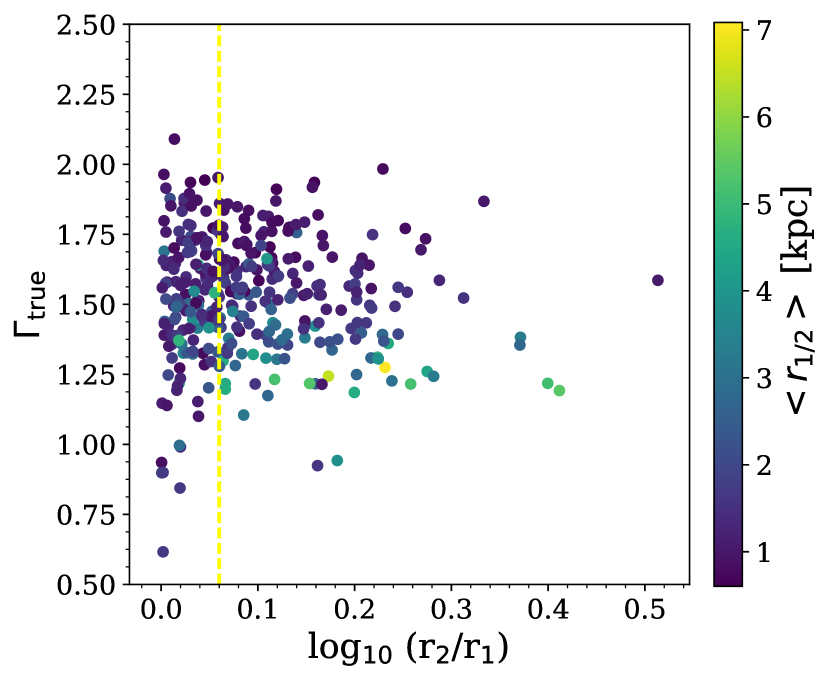
By definition, the value of becomes undefined as the radii of the two metallicity subpopulations coincide, . In selecting our sample, it is therefore imporant to include only galaxies in which the two subpopulations are well separated. We applied the GMM technique to all galaxies in the five high-resolution APOSTLE simulations and, for each, we measured the 3D half-mass radius of the metal-rich and the metal-poor subpopulations and obtained the slope . Fig. A11 shows as a function of the ratio of the 3D half-mass radii of the two metallicity subpopulations. Below 0.06, where is the larger radius of the two, very low values of are obtained. We require > 0.06 for our sample, as shown by the dashed yellow line in Fig. A11.
A2 Subpopulation mixing
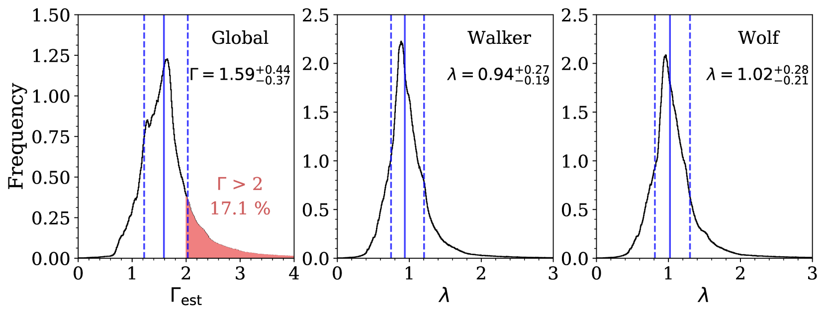
As described in Section 2.2, we define each subpopulation by placing a rigid cut at the intersection of two fitted Gaussians. This treatment ignores mixing between the two subpopulations, which can affect the measurement of the velocity dispersion thus introducing a correlation in the kinematics of the metal-rich and the metal-poor subpopulations. Battaglia et al. (2008), for instance, allow a metallicity gap of . We therefore repeated our analysis, this time taking out one quarter of each subpopulation on both sides of the metallicity cut. The result may be seen in Fig. A12. We obtain = 1.59 and = 0.94 for the Walker et al. (2009) estimator and = 1.02 for the Wolf et al. (2010) estimator when including the metallicity gap. This result is clearly consistent with our previous results for the Walker et al. (2009) and Wolf et al. (2010) estimators when a metallicity gap was not included (Section 3.2).
Appendix B
B1 Numerical convergence of galaxy properties
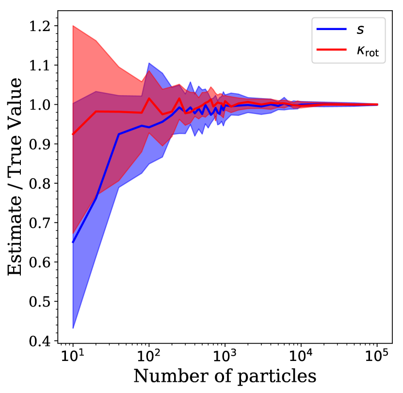
As mentioned in Section 2.2, we require that the galaxies in our sample include over 1000 stellar particles. Since the stellar particles are then split into two metallicity subpopulations, either or both of these subpopulations may end up with a number of particles too small for the properties such as and the sphericity , discussed in Section 5, to numerically converge. We therefore carry out the following test for convergence. We take a sample of 37 dwarfs with stellar particles from the five high-resolution APOSTLE volumes and we calculate the ‘true’ values of and , where we include all particles belonging to the galaxy as defined in Section 2.2. We then take progressively smaller particle samples and recalculate these properties. The result of this test may be seen in Fig. B1, where we show the accuracy of the estimates as a function of the number of particles with which they were calculated. It can be seen that the scatter in the estimate accuracy increases significantly for smaller particle subsamples. The median estimates of are generally accurate, even for 100 stellar particles, while the sphericity, , can be substantially underestimated.
In our sample of 50 dwarfs with two metallicity subpopulations, the minimum number of particles found in an individual subpopulation is just over 400. For this number of particles the estimates are generally accurate, with the 1 scatter of about 5-10 per cent, as can be seen in Fig. B1. We thus conclude that the values of and presented in this work are not affected by the number of particles assigned to individual metallicity subpopulations to any significant extent.
