Modelling of Path Arrival Rate for In-Room Radio Channels with Directive Antennas

Abstract

We analyze the path arrival rate for an inroom radio channel with directive antennas. The impulse response of this channel exhibits a transition from early separate components followed by a diffuse reverberation tail. Under the assumption that the transmitter’s (or receiver’s) position and orientation are picked uniformly at random we derive an exact expression of the mean arrival rate for a rectangular room predicted by the mirror source theory. The rate is quadratic in delay, inversely proportional to the room volume, and proportional to the product of beam coverage fractions of the transmitter and receiver antennas. Making use of the exact formula, we characterize the onset of the diffuse tail by defining a “mixing time” as the point in time where the arrival rate exceeds one component per transmit pulse duration. We also give an approximation for the power-delay spectrum. It turns out that the power-delay spectrum is unaffected by the antenna directivity. However, Monte Carlo simulations show that antenna directivity does indeed play an important role for the distribution of instantaneous mean delay and rms delay spread.

I Introduction

Stochastic models for the channel impulse response are useful tools for the design, analysis and simulation of systems for radio localization and communications. These models allow for tests via Monte Carlo simulation and in many cases provide analytical results useful for system design. Many such models exist for the complex baseband representation of the signal at the receiver antenna ,

$$y(\tau)=\sum_{k}\alpha_{k}s(\tau-\tau_{k}),$$ (1)

where term $k$ has delay $\tau_{k}$ and complex gain $\alpha_{k}$ and $s(\tau)$ is the complex baseband representation of the transmitted signal [1]. These gains and delays form a marked point process with points $\{\tau_{k}\}$ and marks $\{\alpha_{k}\}$. The arrival process $\{\tau_{k}\}$ has an intensity function $\lambda(\tau)$ referred to as the (path) arrival rate [2]. For the most often considered case of uncorrelated zero mean gains, the second moment of the received signal reads

$$\mathds{E}[|y(\tau)|^{2}]=\int_{-\infty}^{\infty}P(\tau-t)|s(t)|^{2}dt,$$ (2)

where the power-delay spectrum, $P(\tau)$, is a product

$$P(\tau)=\sigma_{\alpha}^{2}(\tau)\lambda(\tau),$$ (3)

where $\sigma_{\alpha}^{2}(\tau)$ denotes the variance of a complex gain at a given the delay. A particularly prominent example is the model by Turin [2] where the delays are drawn from a Poisson point process. Although Turin’s model was originally intended for urban radio channels, it has since been taken as basis for a wide range of models for outdoor and indoor channels including the models by, Suzuki [3], Hashemi [4], Saleh and Valenzuela [5], Spencer et al. [6] and Zwick et al. [7, 8]. More recently, this type of statistical channel models has been considered for the millimeter-wave spectrum [9, 10].

Simulations and analyses based on a model are only trustworthy if the parameter settings are properly chosen. For this, empirical methods for estimation of parameters are wide-spread in the literature. Indeed, Turin along with the scientists elaborating this modeling approach [3, 4, 5, 6, 7, 8, 9, 10] determined the parameters based on measurements. The empirical approach, however, gives only limited insight into how model parameters are affected by the propagation environment or system parameters such as frequency bands and antenna configurations. Therefore, costly measurement campaigns performed to determine model parameters for one type of environment for one type of radio system may have to be redone in case the model should be adapted to a different situation, e.g. if considering new frequency bands or different antenna configurations. As a much less explored alternative to the empirical approach, model parameters can in some cases be obtained by analysis of the propagation environment. Potentially, this analytical approach allows us to predict how changes in the propagation environment or in system parameters will affect the channel model parameters. Unfortunately, realistic propagation environments are often too complex to permit such analysis and therefore, we can at best hope to analyze simplistic, but elemental, scenarios. Such elemental results may help us to better understand more realistic scenarios.

The elemental case where one transmitter and one receiver are situated in the same rectangular room has been studied in a number of works [11, 12, 13, 14, 15, 16] channel using the theory of room electromagnetics inspired by the well developed theory of room acoustics [17]. This scenario is relevant since many rooms in old and modern buildings are indeed rectangular. These investigations have focused on determining the reverberation time which characterizes the exponentially decaying reverberation tail of the average power-delay profile, or power-delay spectrum. Room electromagnetics has also been considered as a means to set the parameters of other models through entities derived from the power-delay spectrum [18, 19, 20].

Models of the type (1) are unidentifiable in the power-delay spectrum—according to (3) exactly the same delay-power spectrum can be obtained by a continuum of combinations of arrival rates and conditional mark variances. This effect is clearly present for Turin’s model, but as noted in [21], also holds true for the Saleh-Valenzuela model [5]: by interchanging inter- and intra-cluster parameters for rates and complex gains, and thereby completely altering the model’s behaviour, the same power-delay spectrum is obtained. If two of the three entities related through (3), are specified, the third can be determined. While validated room-electromagnetic models for the delay-power spectrum are already available in the literature. e.g. [11, 12, 13, 14, 15, 16], the room electromagnetic modeling of the arrival rate appears to be still unexplored.

Here, we propose to model for the arrival rate by an analysis inspired by Eyring’s model [22] for reverberation time in room acoustics. Eyring’s model is developed for prediction of reverberation time in rooms with large average absorption coefficient which is the typical situation situation in room electromagnetics [16]. Interestingly, in the process of deriving the reverberation time using an approximation based on mirror source theory, Eyring actually derived an approximation for the arrival rate at large delays for a rectangular room using mirror source theory. According to Eyring’s approximation the arrival rate increases quadratically with delay and is inversely proportional to the room volume. This model thus captures a transition effect of the received signal from early specular contributions to the late diffuse reverberation tail, similar to the effect considered for in-room radio propagation [23, 24, 25, 26]. Eyring’s model for the reverberation time has been recently considered and experimentally validated within room electromagnetics[11, 16] but his results on the arrival rate has not yet been noticed or utilized.

The contributions of the present paper is to adapt Eyring’s analysis to radio channel modeling by including random antenna positions and orientations, as well as to account for antenna directivity. The effect of the antenna directivity on the “richness” of measured impulse responses has been noticed qualitatively in early measurements [27] and the impact of antenna directivity on small scale fading parameters has beed studied in several works [28, 29, 30]. Our approach leads to an exact expression for the mean arrival rate for the mirror source model; for special cases our expression coincide with Eyring’s approximation. The rate is quadratic in delay, inversely proportional to the room volume, and proportional to the product of beam coverage fractions of the transmitter and receiver antennas. Making use of the exact formula, we characterize the onset of the diffuse tail by defining a “mixing time” as the point in time where the arrival rate exceeds one component per transmit pulse duration. We also give an approximation for the power-delay spectrum and study the mean delay and rms delay spread via simulations. It turns out that the power-delay spectrum is unaffected by the antenna directivity, while the mean delay and rms delay spread vary.

We proceed in Section II by introducing the rectangular room considering non-isotropic antennas for which we in Section III detail the mirror source theory. Based on this model, we give approximations in Section IV for the arrival rate and power-delay spectrum. In Section V we analyze the mean arrival rate and power-delay spectrum for random transmitter position and antenna orientation. In Section VI we illustrate the results of the analysis by Monte Carlo simulations. Section VII concludes upon our contributions.

II Considered Rectangular Room and Antennas

Consider a rectangular room illustrated in Fig. 1 with directional transmitter and receiver antennas located inside.

Figure 1: Three-dimensional rectangular room with transmitter and receiver inside along with the coordinate system.

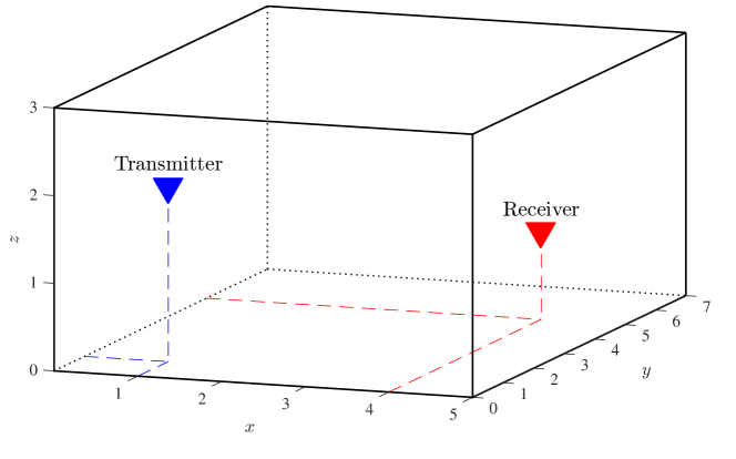
The room is of dimension $L_{x}\times L_{y}\times L_{z}$ and has volume $V=L_{x}L_{y}L_{z}$. The six walls of the room (including floor and ceiling) denoted by $W_{1},\dots,W_{6}$. We assume that the carrier wavelength $l_{c}$ is small compared to the room dimensions, and that only specular reflections occur with a gain independent of incidence direction. The power gain (or reflectance) of wall $i$ is denoted by $g_{i}$ to. Positions are given with reference to a Cartesian coordinate system with origin at one corner and aligned such that the room spans the set $[0,L_{x})\times[0,L_{y})\times[0,L_{z})$. Then the positions of the transmitter and receiver are given as $r_{T}=[x_{T},y_{T},z_{T}]^{T}$ and $r_{R}=[x_{R},y_{R},z_{R}]^{T}$.

To describe the directive antennas, we now introduce a simplistic model. We only define the notations for the transmitter antenna, indicated by subscript $T$; similar entities for the receiver antenna have subscript $R$. For simplicity reason, we ignore polarization of the antennas and describe these by only a directional power gain. We denote the antenna gain by $G_{T}(\Omega)$ (power per solid angle) where the direction specified by the unit vector $\Omega\in\mathbb{S}_{2}$. To simplify notation, we assume the antennas to be lossless, and thus the integral of the antenna gain over the sphere equals $4\pi$. The beam support is the portion of the sphere, denoted by $\Omega_{T}$, is defined as the support of the function $G_{T}(\Omega)$:

$$\Omega_{T}=\{\Omega:G_{T}(\Omega)\neq 0\},$$ (4)

With this definition, the beam coverage solid angle of the transmitter antenna ranging from zero to $4\pi$ reads

$$|\Omega_{T}|=\int_{\mathbb{S}_{2}}\mathds{1}(\Omega\in\Omega_{T})d\Omega,$$ (5)

where $\mathds{1}(\cdot)$ denotes an indicator function with value one if the argument is true and zero otherwise. To shorten the notation, we further define the beam coverage fraction as

$$\omega_{T}=\frac{|\Omega_{T}|}{4\pi}$$ (6)

The beam coverage fraction ranges from zero to one and can be interpreted as the probability that a wave impinging from a uniformly random direction is within the antenna beam.

III Mirror Sources and Multipath Parameters

For the defined setup, mirror source theory predicts that the received signal is an infinite sum of attenuated, phase-shifted and delayed signal components as in (1). Unlike Turin’s model, in this case the pairs of delay and complex amplitudes $\{(\tau_{k},\alpha_{k})\}$ do not form a marked Poisson process but are given by the geometry of the propagation environment. The complex gains and delays are readily described using the theory of mirror sources as follows.

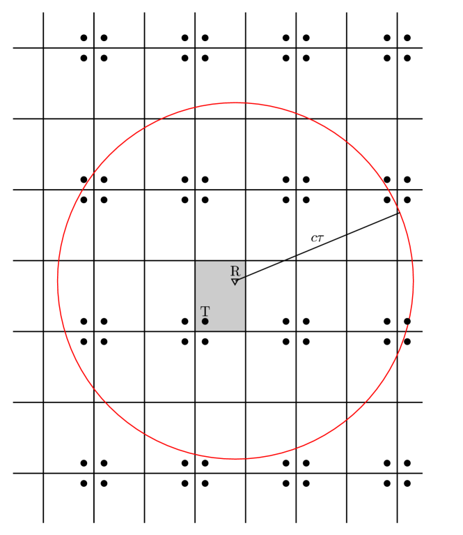
To construct the path from $T$ to $R$ via a single reflection at wall $W$ we determine the position of mirror source $T^{\prime}$ by mirroring $T$ in $W$. Thereby, the interaction point can be determined as the wall’s intersection with the straight line segment from $T^{\prime}$ to $R$. The two-bounce path $T-W_{1}-W_{2}-R$ may be constructed by mirroring wall $W_{1}$ in wall $W_{2}$ to construct $W_{1}^{\prime}$ and then mirroring $T^{\prime}$ in $W_{1}^{\prime}$. By repeating this procedure ad infinitum we can construct and infinite set of mirror sources and mirror rooms as illustrated in Figure 2. The position of mirror source $k$ can be computed as

$$r_{T(k_{x},k_{y},k_{z})}=\begin{bmatrix}\big{\lceil}\tfrac{k_{x}}{2}\big{\rceil}\cdot 2L_{x}+(-1)^{k_{x}}\cdot x_{T}\\ \big{\lceil}\tfrac{k_{y}}{2}\big{\rceil}\cdot 2L_{y}+(-1)^{k_{y}}\cdot y_{T}\\ \big{\lceil}\tfrac{k_{z}}{2}\big{\rceil}\cdot 2L_{z}+(-1)^{k_{z}}\cdot z_{T}\end{bmatrix}$$ (7)

where $k_{x}$ is the number of reflections on the two walls parallel to the $y-z$-plane, and similarly for $k_{y},k_{z}$. Hence, the path index path index $k$ corresponds to a triplet $k=(k_{x},k_{y},k_{z})$. Alternatively, the same path can be constructed by introducing a mirror receiver at position $r_{Rk}$ determined by replacing subscript $T$ by subscript $R$ in (7). Notice the direct (or line-of-sight) path is also included for $k=(0,0,0)$, since for this case $r_{T(0,0,0)}=r_{T}$ and $r_{R(0,0,0)}=r_{R}$. For notational brevity, we use subscript $k=0$ instead of $k=(0,0,0)$ for entities related to the direct path throughout the paper.

The signal emitted by mirror source $k$ arrives at the receiver with delay $\tau_{k}$. Analogously, the signal emitted by the transmitter observed by mirror receiver $k$ has the same delay $\tau_{k}$. The delay of path $k$ be computed from the positions of mirror source $k$ or mirror receiver $k$ as

$$\tau_{k}=\|r_{Tk}-r_{R}\|/c=\|r_{Rk}-r_{T}\|/c,$$ (8)

where $c$ is the speed of light.

The directions of departure and arrival for each path can also be computed. The direction of arrival of the signal from mirror source $k$ is given by the unit vector

$$\Omega_{Rk}=\frac{r_{Tk}-r_{R}}{\|r_{Tk}-r_{R}\|}.$$ (9)

Similarly, the direction of departure of path $k$ denoted by $\Omega_{Tk}$ and can be computed from (9) by interchanging subscripts $T$ and $R$. It follows that directions of departure and arrival of a specific path are related as

$$\Omega_{Tk} =-\begin{bmatrix}(-1)^{k_{y}+k_{z}}&&\\ &(-1)^{k_{x}+k_{z}}&\\ &&(-1)^{k_{x}+k_{y}}\end{bmatrix}\Omega_{Rk}.$$ (10)

In particular, for the direct path $\Omega_{T0}=-\Omega_{R0}$.

Figure 2: The rectangular room seen from above with transmitter $T$ and a receiver $R$ and a number of mirror rooms. The pattern continues similarly in the direction perpendicular to the drawing plane. Contributions from mirror sources inside the sphere of radius $c\tau$ arrive at the receiver at delays smaller than $\tau$.

Finally, the gain of path $k$ can be specified. We shall not be concerned with the phase of the complex gain $\alpha_{k}$, but only its squared magnitude, i.e. the corresponding power gain. The power gain of path $k$ reads

$$|\alpha_{k}|^{2} =g_{k}\cdot\frac{G_{T}(\Omega_{Tk})G_{R}(\Omega_{Rk})}{(4\pi c\tau_{k}/l_{c})^{2}}$$ (11)

where the factor $g_{k}$ denotes the gain due to reflections on the walls, the numerator accounts for the transmitter and receiver antennas, and the denominator is due to the attenuation of a spherical wave with $l_{c}$ denoting the wavelength. Naming the walls parallel to the $yz$-plane as $W_{1}$ and $W_{2}$ respectively, we see that path $k$ interacts with wall $W_{1}$ in total $\big{|}\lfloor\tfrac{k_{x}}{2}\rfloor\big{|}$ times and with wall $W_{2}$ in total $\big{|}\lceil\tfrac{k_{x}}{2}\rceil\big{|}$ times. The numbers of interactions with other walls are computed similarly. Consequently,

$$g_{k}=g_{1}^{\big{|}\lfloor\tfrac{k_{x}}{2}\rfloor\big{|}}g_{2}^{\big{|}\lceil\tfrac{k_{x}}{2}\rceil\big{|}}g_{3}^{\big{|}\lfloor\tfrac{k_{y}}{2}\rfloor\big{|}}g_{4}^{\big{|}\lceil\tfrac{k_{y}}{2}\rceil\big{|}}g_{5}^{\big{|}\lfloor\tfrac{k_{z}}{2}\rfloor\big{|}}g_{6}^{\big{|}\lceil\tfrac{k_{z}}{2}\rceil\big{|}}.$$ (12)

Henceforth, we consider for simplicity all walls to have the same gain value $g=g_{1}=\dots=g_{6}$. Then the gain of path $k$ simplifies as $g_{k}=g^{|k|}$ with the convention $|k|=|k_{x}|+|k_{y}|+|k_{z}|$. Furthermore, we remark that for the direct path the expression (11) reduces to the Friis equation [31] for propagation in free space.

III-A Numerical Examples

Before proceeding with analysis of the mirror source model, we first illustrate how the received signal behaves with a few numerical examples. The settings are specified in Table I. The transmitter and receiver have identical sector antennas. The transmit antenna gain is

$$G_{T}(\Omega)=\frac{1}{\omega_{T}}\mathds{1}(\Omega^{T}\zeta_{T}\geq 1-2\omega_{T}),$$ (13)

i.e. the gain is constant over the spherical cap centered at the direction given by the unit vector $\zeta_{T}$. This implies a half-beam width of $\arccos(1-2\omega_{T})$. The receiver antenna is defined similarly. In this example, we orient the antennas in direction of line-of sight, i.e. $\zeta_{T}=\Omega_{T0}$ and $\zeta_{R}=\Omega_{R0}$. The transmitted signal $s(t)$ is a sinc pulse which has constant Fourier transform over the considered frequency bandwidth, and zero elsewhere.

Figure 3: Examples of magnitude square of received signal for four different $\omega_{T}\omega_{R}$ values for the setup given in Table I. The antennas are located at $r_{T}=[2.5,2.5,1.5]^{T}\mathrm{m}$ and $r_{R}=[3.8,4.0,0.6]^{T}\mathrm{m}$ and are oriented exactly in the direction of line-of-sight.

TABLE I: Simulation Settings

Room dim., $L_{x}\times L_{y}\times L_{z}$	$5\times 5\times 3\,\mathrm{{}^{3}}\mathrm{m}$
Reflection gain, $g$	$0.6$
Center Frequency	$60\,\mathrm{G}\mathrm{Hz}$
Bandwidth, $B$	$2\,\mathrm{G}\mathrm{Hz}$
Speed of light, $c$	$3\cdot 10^{8}\,\mathrm{m}\mathrm{/}\mathrm{s}$

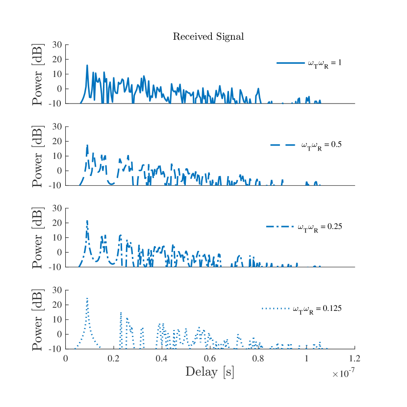
Fig. 3 shows received signals for four different antenna settings; isotropic antennas ($\omega_{T}\omega_{R}=1$), and three cases with directive antennas. The general trend is that the received signal decays exponentially with delay while the signal contributions gradually merge into a diffuse tail. The rate of diffusion depends on the antenna directivity: higher antenna directivity leads to a slower diffusion process.

IV Analysis of Deterministic Mirror Source Model

The equations (7)–(12) define the mirror source model to an extent where the model can be simulated from, but are difficult to interpret directly. To better understand the behavior of the model we next consider approximations for the arrival count, arrival rate and power-delay spectrum. In this section assume the antenna positions and orientations as deterministic. Later, in Section V, we randomize these variables.

IV-A Arrival Count

The arrival count $N(\tau)$ is defined as the number of paths contributing to the received signal components up to and including a certain time $\tau$. For a path to contribute, the corresponding mirror source should be within a radius $c\tau$ of the receiver, see Fig. 2. Furthermore, the path should be within the beam support of both the transmitter and receiver antennas. Thus the arrival count can be expressed as

$$N(\tau) =\sum_{k}\mathds{1}(\tau_{k}\leq\tau)\cdot\mathds{1}(\Omega_{Tk}\in\Omega_{T})\cdot\mathds{1}(\Omega_{Rk}\in\Omega_{R})$$ (14)

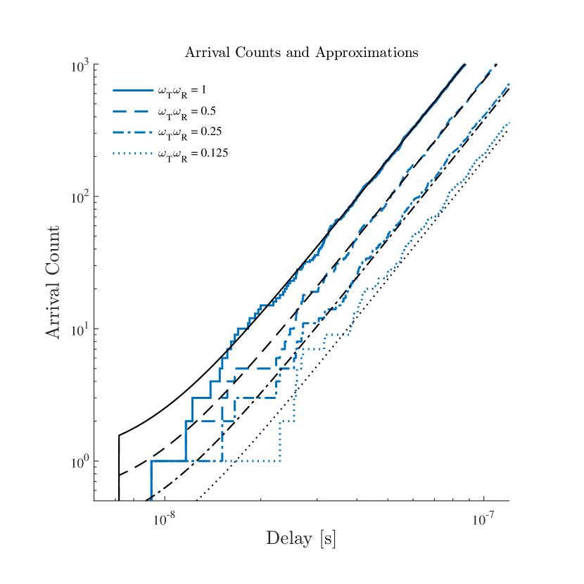
The count depends on the antenna positions, orientations and as exemplified in Fig. 4, on the specific antennas. As can be seen from the example, the count approaches a cubic asymptote for large delays. This cubic trend was noticed and approximated by Eyring as [22]

$$N(\tau)\approx\frac{4\pi c^{3}\tau^{3}}{3V},\qquad\tau\gg 0.$$ (15)

Figure 4: Arrival counts (blue lines) and corresponding approximation obtained from (18) (black lines) corresponding to the examples in Fig. 3.

We now develop an approximation for the arrival count by adapting Eyring’s analysis to the current setting. First, we approximate the term due to the direct path as

$$\mathds{1}(\tau_{0}\leq\tau)\omega_{T}\omega_{R}$$ (16)

Secondly, the number of mirror sources with delay less than $\tau$ equals the number of mirror sources inside the sphere with radius $c\tau$ centered at the receiver. For $c\tau$ large compared to the diagonal of the room, i.e. $c\tau\gg\sqrt{L_{x}^{2}+L_{y}^{2}+L_{z}^{2}}$, the number of such mirror sources is approximately

$$\frac{4\pi c^{3}(\tau^{3}-\tau_{0}^{3})}{3V}$$ (17)

where we include one mirror source per room volume and subtract the contribution due to the volume closer than $c\tau_{0}$ to the receiver. Fourthly, only a fraction, $\omega_{R}$, of these mirror sources are picked up by the receiver. Ignoring the dependency between the direction of departure and arrival for indirect components, we account for the transmit antenna by a factor $\omega_{T}$. From this reasoning we have

$$N(\tau) \approx\mathds{1}(\tau\geq\tau_{0})\left[1+\frac{4\pi c^{3}(\tau^{3}-\tau_{0}^{3})}{3V}\right]\omega_{T}\omega_{R}.$$ (18)

As exemplified in Fig. 4 this approximation follows closely the asymptote of the exact count. For the special case of isotropic and colocated antennas expression (18) equals Eyring’s approximation (15) plus one.

IV-B Arrival Rate

The arrival rate, denoted by $\lambda(\tau)$, is expected number of signal components arriving at the receiver per unit time at delay $\tau$ which can be defined it terms of the arrival count such that the expression

$$\mathbb{E}[N(\tau)]=\int_{-\infty}^{\tau}\lambda(t)dt$$ (19)

holds true. Essentially, $\lambda(\tau)$ can be thought of as a “derivative” of $\mathbb{E}[N(\tau)]$. However, since the count $N(t)$ is deterministic, we see that $\mathbb{E}[N(\tau)]$ equals $N(\tau)$. The count is a step function and therefore $\lambda(\tau)$ should be interpreted in the distribution sense as a Radon-Nikodym derivative (with respect to Lebesque measure) which leads to:

$$\lambda(\tau)=\sum_{k}\delta(\tau-\tau_{k})\cdot\mathds{1}(\Omega_{Tk}\in\Omega_{T})\cdot\mathds{1}(\Omega_{Rk}\in\Omega_{R}),$$ (20)

where $\delta(\cdot)$ is Dirac’s delta function. Again, the exact count yields no valuable interpretation. Instead by inserting the approximation (18) for the arrival count into (19) we approximate the arrival rate as

$$\lambda(\tau)\approx\delta(\tau-\tau_{0})\omega_{T}\omega_{R}+\mathds{1}(\tau>\tau_{0})\frac{4\pi c^{3}\tau^{2}}{V}\omega_{T}\omega_{R}.$$ (21)

The approximation (21) is clearly not valid point-wise, but should be seen as the average number of arrivals per time unit in a small time interval centered at $t$.

The expression (21) gives rise to a number of observations. First, the arrival rate is quadratic in delay which is in sharp contrast to the widespread Saleh-Valenzuela model [5] where the delays of each “cluster” of components has constant arrival rate. Moreover, considering that clusters also arrive at constant rate, the overall arrival rate is only linearly increasing in delay [21]. Secondly, the arrival rate in (21) is inversely proportional to the room volume for $\tau>\tau_{0}$. Thus, larger rooms lead to smaller arrival rates. This implies that attempts to empirically characterize arrival rates for inroom channels should pay attention to the room size. Finally, we observe that the antennas affect the arrival rate by a delay-independent scaling. Thus very directive antennas lead to a sparser channel in the early part of the channel response, in agreement with experimental results presented in [27, 28, 29, 30]. However, the arrival rate still grows quadratically and eventually the components in the response merge into a diffuse tail.

IV-C Approximation for Power-Delay Spectrum

We now derive an approximation of the power-delay spectrum. Eyring noted in [22] that the number of wall interactions for mirror source $k$ is roughly

$$|k|\approx\tau_{k}\cdot\frac{cS}{4V},\quad k\neq(0,0,0).$$ (22)

with $S=2(L_{x}L_{y}+L_{x}L_{z}+L_{y}L_{z})$ denoting the surface area of the room. Inserting this into (11) yields (for $g=g_{1}=\dots=g_{6}$)

$$|\alpha_{k}|^{2}\approx\begin{cases}g^{\tau_{k}cS/4V}\cdot\frac{G_{T}(\Omega_{Tk})G_{R}(\Omega_{Rk})}{(4\pi c\tau_{k}/l_{c})^{2}},&k\neq(0,0,0)\\ \frac{G_{T}(\Omega_{T0})G_{R}(\Omega_{R0})}{(4\pi c\tau_{0}/l_{c})^{2}},&k=(0,0,0)\end{cases}$$ (23)

For propagation paths with large delay, the direction of departure and arrival are close to uniformly distributed on the sphere. Thus we approximate the gain due to the transmitter antenna for a direction of departure within the beam coverage solid angle as

$$\frac{1}{|\Omega_{T}|}\int_{\Omega_{T}}G_{T}(\Omega)d\Omega=\frac{1}{|\Omega_{T}|}\int_{\mathbb{S}_{2}}G_{T}(\Omega)d\Omega=\frac{1}{\omega_{T}}$$ (24)

A similar expression is obtained at the receiver side. Now, further assuming independent directions of departure and arrival, we have for the conditional second moment,

$$\sigma_{\alpha}^{2}(\tau)\approx\begin{cases}\frac{g^{\tau cS/4V}}{(4\pi c\tau/l_{c})^{2}}\cdot\frac{1}{\omega_{T}\omega_{R}}&\tau>\tau_{0}\\ \frac{1}{(4\pi c\tau/l_{c})^{2}}\cdot\frac{1}{\omega_{T}\omega_{R}}&\tau=\tau_{0}.\end{cases}$$ (25)

Combining with the expression for the arrival rate, the approximation for the power-delay spectrum reads

$$P(\tau)\approx\delta(\tau-\tau_{0})\frac{1}{(4\pi c\tau_{0}/l_{c})^{2}}+\mathds{1}(\tau>\tau_{0})\frac{e^{-\tau/T}}{4\pi V/l_{c}^{2}c}$$ (26)

with the reverberation time $T$ defined as

$$T=-\frac{4V}{cS\ln(g)}.$$ (27)

This expression for the power-delay spectrum is remarkable in a number of ways. First, the form of the power-delay spectrum appears to be a spike plus an exponential tail. This is interesting in the light of the super-exponential decay of the per-path gain in (25). However, this super-exponential trend is balanced out by the quadratic increase in arrival rate such that the net result is an exponential decay. Second, the positions of the transmitter and receiver antennas only enter via the delay of the direct component. This implies the expected result that the decay rate of the tail is constant throughout the whole room as is well known in room electromagnetics. However, the onset of the tail depends on the delay of the direct component. This exact structure was the one studied in great detail in [20]. Third, the power-delay spectrum appears to be unaffected by the directivity of the antenna. Indeed, the antennas enter in both the arrival rate and in the conditional gain, but the effects cancel in the power-delay spectrum.

The approximation in (23) can be made more accurate by incorporating more complex models such as the ones developed for room acoustics, see [32, 17]. As an example, the modification introduced in [17] accounts for this discrepancy due to the approximation in (22) where a random variable is replace by its mean. This modification amounts to adjusting the reverberation time by a correction factor $\xi$ defined as

$$\xi=\frac{1}{1+\gamma^{2}\ln(g)/2}.$$ (28)

where the constant $\gamma^{2}$, which depends on the aspect ratio of the room, can be determined by Monte Carlo simulation and typically takes values in the range 0.3 to 0.4 [17]. The particularities of such corrections are of less importance for the forthcoming analysis and therefore further refinements of (28) are left as future work.

V Analysis of Randomized Mirror Source Model

In the previous section, antenna positions and orientations were held fixed. In the sequel, we let let the position and orientation of the transmitter be random.

V-A Mean Arrival Count and Arrival Rate

Suppose that the position and orientation of the receiver antenna is fixed. In contrast hereto, the transmitter’s position is random with a uniform distribution on the room, i.e. that $r_{T}\sim\mathcal{U}([0,L_{x}]\times[0,L_{y}]\times[0,L_{z}])$. Furthermore, let the transmitter’s orientation be random according to a uniform distribution on the sphere. The counting variable $N(\tau)$ is random with mean

$$\mathbb{E}[N(\tau)] =\mathbb{E}\big{[}\sum_{k}\mathds{1}(\tau_{k}<\tau)\cdot\mathds{1}(\Omega_{Tk}\in\Omega_{T})\cdot\mathds{1}(\Omega_{Rk}\in\Omega_{R})].$$ (29)

Since the orientation of the transmitter antenna is uniformly random, the probability for any particular fixed direction, to reside in the random beam support $\Omega_{T}$, equals the beam coverage fraction $\omega_{T}$. Thus, we have the conditional mean

$$\mathbb{E}[\Omega_{Tk}\in\Omega_{T}|\Omega_{Tk}]=\omega_{T}$$ (30)

irrespective of the particular value of $\Omega_{Tk}$. Each mirror sources is uniformly distributed within its mirror room, and therefore mirror source positions constitue a homogeneous (but not Poissonian) random spatial point process with intensity $1/V$. Then, inserting (30) and using Campbell’s theorem[33], we can rewrite the expectation as an integral over mirror source positions

$$\mathbb{E}[N(\tau)] =\frac{\omega_{T}}{V}\int\mathds{1}\left(\tfrac{\|r-r_{R}\|}{c}<\tau\right)\mathds{1}\left(\tfrac{r-r_{R}}{\|r-r_{R}\|}\in\Omega_{R}\right)dr$$

$$=\frac{4\pi c^{3}\tau^{3}}{3V}\omega_{T}\omega_{R}\mathds{1}(\tau>0).$$ (31)

Taking the derivative of the expected arrival count, we obtain the corresponding arrival rate

$$\lambda(\tau)=\frac{4\pi c^{3}\tau^{2}}{V}\omega_{T}\omega_{R}\mathds{1}(\tau>0).$$ (32)

It follows by simple modifications of the above argument that the same results hold true for a number of different cases:

1. Uniform receiver orientation and transmitter fixed orientation and uniform location.

2. Either of the antennas are isotropic and either of the antenna location are uniform.

3. Transmitter position and orientation are uniform and independent of the receiver position and orientation.

4. Transmitter position and antenna orientation are uniform conditioned on the receiver position and orientation.

Obviously, Case 4) implies Cases 1) through 3). Moreover, by symmetry, any of the above results hold true if the transmitter and receiver swap roles.

This quadratically increasing rate bears witness of the gradual transition in the impulse response that consists of separate specular components at early delays to a late diffuse tail consisting of myriads of specular components. We remark that for isotropic antennas Eyring’s approximation (see (15)) is equal to our expression for the mean count. In this sense, Eyring’s approximation is not only valid asymptotically, but is exact in the mean. The inclusion of the beam coverage fractions is a natural extension to the non-isotropic case.

The relative ease by which we derived the mean arrival count (31) may lead us to think that perhaps also higher moments could be easily derived. However, it proves much more challenging to derive its second moment—in fact we have not been able to establish an exact expression. We give an approximation in Appendix A. Similarly, it is difficult to get exact formulas if less randomness is introduced in the model. To that end, Appendix B gives an upper bound to the mean arrival rate for the case where the transmitter antenna has random position, but fixed orientation; Appendix C gives an approximation for the mean count for fixed transmitter-receiver distance.

V-B Mixing Time

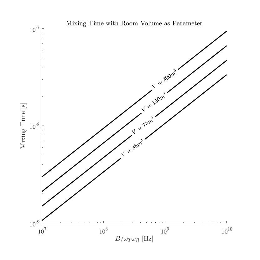
The arrival rate gives us a way to quantify the onset of this diffuse tail, i.e. the point in time from which the preceding signal components merge together and can no longer be distinguished. In analogy with room acoustics literature, see [34], we refer to this time as the “mixing time” which we denote by $\tau_{\mathrm{mix}}$. For a system with signal bandwidth $B$ in which the receiver can distinguish on average one signal component per pulse duration $1/B$, then we have $\lambda(\tau_{\mathrm{mix}})=B$, and the mixing time can be expressed as

$$\tau_{\mathrm{mix}}=\sqrt{\frac{BV}{4\pi c^{3}\omega_{T}\omega_{R}}}.$$ (33)

The mixing time is proportional to the square root of the room volume which is quite intuitive: larger rooms have longer mixing times. Moreover, the mixing time is inversely proportional to the square root of the beam coverage fractions: more directive antennas lead to a later onset for the diffuse tail. Finally, by increasing the system bandwidth, the mixing time increases by the square root of the bandwidth. The mixing time determines if a diffuse reverberation tail can be observed in noise limited measurements. The diffuse tail appears only if the power-delay spectrum exceeds the noise floor at the mixing time, and is otherwise masked by noise.

As an example, the setup with the settings given in Table I gives a mixing time of $21\ \mathrm{n}\mathrm{s}$ for isotropic antennas and $42\ \mathrm{n}\mathrm{s}$ for hemisphere antennas. Fig. 5 shows the mixing time versus $B/\omega_{T}\omega_{R}$ for a range of room volumes.

Figure 5: Mixing time versus $B/\omega_{T}\omega_{R}$ for different room volumes.

V-C Approximation for Power-Delay Spectrum

By following essentially the same steps leading to the approximation (26) we can derive an approximation for the power-delay spectrum. For simplicity, however, we ignore here the different gain of the direct path and assign instead the same gain as any other path. Thus the conditional second moment for the path gain reads

$$\sigma_{\alpha}^{2}(\tau)\approx\frac{g^{\tau cS/4V}}{(4\pi c\tau/l_{c})^{2}}\cdot\frac{1}{\omega_{T}\omega_{R}}$$ (34)

Combining this with the arrival rate in (32), we obtain

$$P(\tau)\approx\mathds{1}(\tau>0)\frac{e^{-\tau/T}}{4\pi V/l_{c}^{2}c}.$$ (35)

with the reverberation time $T$ defined in (27) with correction factor in (28).

VI Simulation Study

We now illustrate the theoretical results derived in the previous sections by comparing them with Monte Carlo simulations. We use nearly the same setup as in the numerical examples provided earlier in Section III-A with the same settings listed in Table I. Compared to the previous setup, there are two differences: 1) the transmitter and receiver are placed uniformly at random within the room and 2) orientations picked uniformly at random, i.e. we simulate the setup leading to (31) and (32). We perform 10 000 Monte Carlo simulation runs.

Fig. 6 reports individual realizations and mean arrival counts for three different antenna settings. From the realizations depicted in the upper panel it is evident that the arrival count varies between realizations and that this variation is more pronounced for more directive antennas. Moreover, the realizations tend to the mean value at large delays. The lower panel compares the theoretical expressions for the mean count (31) with the Monte Carlo estimates. As expected, the corresponding curves fit almost perfectly.

Figure 6: Realizations of arrival count for random transmitter and receiver position and orientation (upper panel) and mean arrival count (lower panel).

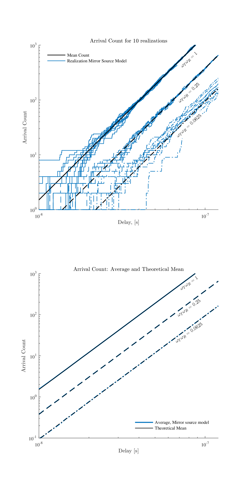
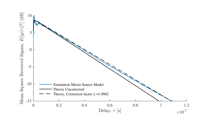
Fig. 7 shows the expected power of the received signal, i.e. $\mathbb{E}[|y(t)|^{2}]$, computed using the Monte Carlo simulation. For clarity, only the results for isotropic antennas are shown; the curves for the non-isotropic antennas are identical modulo uncertainties due to the Monte Carlo simulation technique. This observation confirms the observation made in the introduction that models with very different arrival rates, e.g. due to differences in antenna directivity, can indeed lead to the same power-delay spectrum. The simulation is compared with the approximation obtained by using (2) and (35). From Fig. 7 it appears that the slope of the theoretical curve, i.e. the reverberation time computed in (27), deviates from the simulation by about 9 %. The fit can be improved by applying the correction factor (28). According to [17], the value $\gamma^{2}=0.35$ can be used for the aspect ratio of the room considered. For our simulation setup, this yields a correction factor of $\xi\approx 1.0982$ which gives an excellent fit.

Figure 7: Mean square received signal.

Figure 8: Empirical cumulative probability of instantaneous mean delay (upper panel) and rms delay spread (lower panel) with $\omega_{T}\omega_{R}$ as parameter.

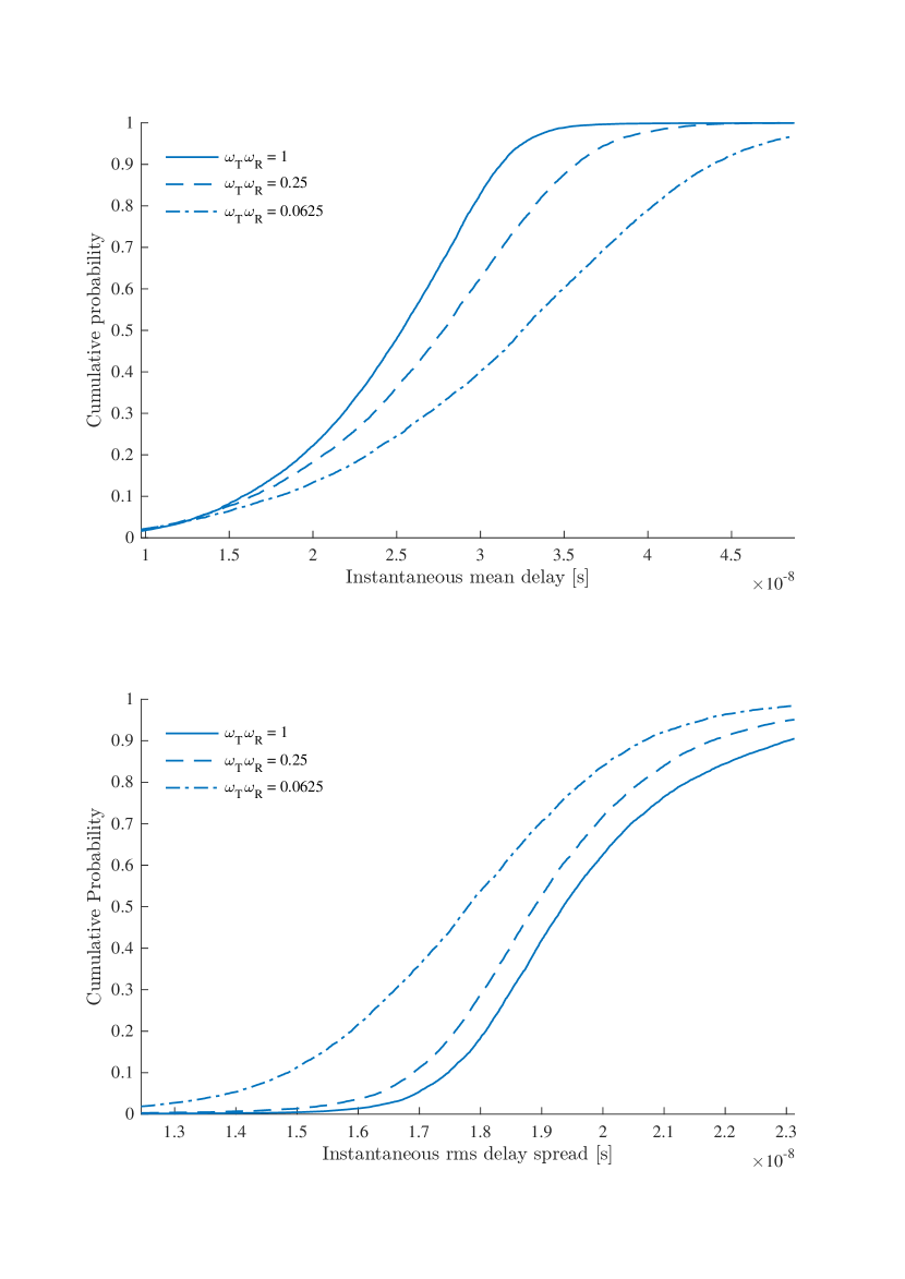
The instantaneous mean delay and rms delay spread are often considered as important parameters for design of radio systems. Theoretical analysis of these entities is beyond the scope of this contribution, but we report some simulated empirical cumulative distribution functions in Fig. 8 with $\omega_{T}\omega_{R}$ as parameter. To limit the computational complexity, only components with a delay less that 120  n s  are simulated. In these simulations the mean delay and rms delay spread are computed as respectively the first and centered second moments of the realizations of $|y(t)|^{2}$ (thus including the effect of the transmitted pulse). Even though the antenna directivity does not affect the power delay spectrum, it is apparent from Fig. 8 that the instantaneous mean delay and rms delay spread vary significantly with the antenna directivity.

VII Conclusion

The present study shows how the path arrival rate can be analyzed based on mirror source theory for rectangular room. Directivity of the transmitter and receiver antennas is accounted for by incorporating a simplified antenna model. For this setup we give an exact formula for the mean arrival count and consequently for the arrival rate for the case where the position and orientation of the transmitter are uniformly random. The rate grows quadratically with delay giving rise to a transition from early isolated signal components gradually merging into a diffuse reverberation tail at later delays. The rate is inversely proportional to the room volume, and thus larger rooms lead to a slower transition. Moreover, the rate is proportional to the product of beam coverage fractions of the transmitter and receiver antennas, and thus more directive antennas yield lower arrival rate. The derived expression quantifies the impact of directive antennas on the arrival rate, a phenomenon observed qualitatively in a number of previous experimental and simulation studies in the literature.

We present two immediate application of the expression of the arrival rate. First, we derive a simple formula for the “mixing time”, i.e. the point in time at which the mean arrival rate exceeds one component per transmit pulse duration. The mixing time quantifies to what extent non-overlapping signal components is to be expected for a given scenario. Second, we use our expression to approximate the power delay spectrum which appears to be unaffected by the antenna radiation pattern. However, the antennas do indeed play an important role for the distribution of instantaneous mean delay and rms delay spread as shown by Monte Carlo simulations.

The motivation for this work was to achieve calibration of the arrival rate used in stochastic radio channel models based on geometric considerations rather than empirically. Indeed this method seems to be feasible for obtaining models of simplified structures such as the rectangular room considered here. The results obtained in the simplified settings may be used as building blocks for constructing more for more complex radio propagation environments.

Appendix A Second Moment of Arrival Count

The raw second moment of the arrival count reads

$$\mathbb{E}[N(\tau)^{2}]= \sum_{k,k^{\prime}}\mathbb{E}[N_{k}N_{k^{\prime}}],$$ (36)

with the shorthand notation

$$N_{k}=\mathds{1}(\tau<\tau_{k})\mathds{1}(\Omega_{Tk^{\prime}}\in\Omega_{T})\mathds{1}(\Omega_{Rk^{\prime}}\in\Omega_{R})].$$ (37)

Noting that $N_{k}^{2}=N_{k}$, we see that the sum of diagonal terms ($k=k^{\prime}$) equals the mean $\mathbb{E}[N(\tau)]$ and thus

$$\mathbb{E}[N(\tau)^{2}]= \mathbb{E}[N(\tau)]+\sum_{k\neq k^{\prime}}\mathbb{E}[N_{k}N_{k^{\prime}}].$$ (38)

The cross terms $(k\neq k^{\prime})$, cannot be readily computed. Instead, we approximate the cross terms by considering the positions of the mirror to be uncorrelated:

$$\mathbb{E}[N(\tau)^{2}]\approx \mathbb{E}[N(\tau)]+\sum_{k,k^{\prime}}\mathbb{E}[N_{k}]\mathbb{E}[N_{k^{\prime}}]$$ (39)

$$= \mathbb{E}[N(\tau)]^{2}+\sum_{k}(\mathbb{E}[N_{k}]-\mathbb{E}[N_{k}]^{2}).$$ (40)

The terms in the last sum are variances of $N_{k}$ of which most vanish. Only mirror rooms which can be intersected by a sphere of radius $c\tau$ centered at the receiver contribute to this sum. Considering a receiver at the center of the room, for these mirror rooms,

$$\tau-D/2c<\tau_{k}<\tau+D/2c$$ (41)

where $D=\sqrt{L_{x}^{2}+L_{y}^{2}+L_{z}^{2}}$ is the length of the main diagonal of the room. The number of such mirror rooms can be approximated as

$$\mathbb{E}[N(\tau+D/(2c))]-\mathbb{E}[N(\tau-D/(2c))]$$ (42)

Finally, approximating the values of the variances by the maximal variance of a Bernoulli variable, we have

$$\mathbb{E}[N(\tau)^{2}]\approx \mathbb{E}[N(\tau)]^{2}$$ (43)

$$+\frac{1}{4}(\mathbb{E}[N(\tau+\frac{D}{2c})]-\mathbb{E}[N(\tau-\frac{D}{2c})])$$ (44)

Monte Carlo simulations (not reported here) for the setup described in Section VI demonstrate that the approximation is reasonably accurate for the raw moment, but overshoots the variance significantly.

Appendix B Transmitter with Random Position and Fixed Orientation

Let the transmitter’s orientation be fixed, but its position be uniformly distributed.The position and orientation of the receiver is fixed. Then the mean arrival count reads

$$\mathbb{E}[N(\tau)] =\mathbb{E}\big{[}\sum_{k}\mathds{1}(\tau_{k}<\tau)\cdot\mathds{1}(\Omega_{Tk}\in\Omega_{T})\cdot\mathds{1}(\Omega_{Rk}\in\Omega_{R})\big{]}$$

$$\leq\mathbb{E}\big{[}\sum_{k}\mathds{1}(\tau_{k}<\tau)\cdot\mathds{1}(\Omega_{Rk}\in\Omega_{R})\big{]}$$ (45)

with equality for isotropic transmitter antenna. By Campbell’s theorem,

$$\mathbb{E}[N(\tau)] \leq\frac{1}{V}\int\mathds{1}\left(\tfrac{\|r-r_{R}\|}{c}<\tau\right)\mathds{1}\left(\tfrac{r-r_{R}}{\|r-r_{R}\|}\in\Omega_{R}\right)dr$$

$$=\frac{4\pi c^{3}\tau^{3}}{3V}\cdot\omega_{R}\mathds{1}(\tau>0).$$ (46)

Symmetry gives a similar inequality involving $\omega_{R}$. In combination, these two lower bound yields

$$\mathbb{E}[N(\tau)] \leq\frac{4\pi c^{3}\tau^{3}}{3V}\cdot\min\{\omega_{T},\omega_{R}\}\mathds{1}(\tau>0),$$ (47)

again, with equality obtained either of the antennas are isotropic. Since (47) holds for all $\tau$, the arrival rate is upper bounded as

$$\lambda(\tau)\leq\frac{4\pi c^{3}\tau^{2}}{V}\cdot\min\{\omega_{T},\omega_{R}\}\mathds{1}(\tau>0).$$ (48)

with equality if either of the antennas are isotropic.

We remark that by symmetry, the bounds (47) and (48) hold true if we instead let position of the receiver be uniformly distributed within the room and the transmitters be fixed. Furthermore, it can be shown by some adaptation of the proof that the bound also holds in the case where both transmitter and receiver have independent and uniformly distributed but fixed orientations.

Appendix C Deterministic Transmitter-Receiver Distance

To compute the mean arrival count for fixed transmitter-receiver distance we need to compute a conditional expectation. However, the condition renders the calculation of the mean count very cumbersome if at all possible. Instead, we approximate the expected count as motivated by the following reasoning. First, the conditional arrival count is strictly zero for $\tau<\tau_{0}$. Second, due to the random orientation of antennas, the direct component $\tau=\tau_{0}$ occurs with probability $\omega_{T}\omega_{R}$. Third, conditioning on $\tau_{0}$ does not change the fact that there is exactly one mirror source per mirror room. Therefore, the mean count for $c\tau$ much greater than the diagonal of the room remains the same as in the unconditional case. Thus, we have the approximation for the conditional mean arrival count

$$\mathbb{E}[N(\tau)|\tau_{0}]\approx\mathds{1}(\tau\leq\tau_{0})\left(1+\frac{4\pi c^{3}(\tau^{3}-\tau_{0}^{3})}{3V}\right)\omega_{T}\omega_{R}$$ (49)

with corresponding conditional arrival rate

$$\lambda(\tau|\tau_{0})\approx\delta(\tau-\tau_{0})\omega_{T}\omega_{R}+\mathds{1}(\tau>\tau_{0})\frac{4\pi c^{3}\tau^{2}}{V}\omega_{T}\omega_{R}.$$ (50)

The right hand side of (49) coincides with that of the approximation obtained in the case with non-random transmitter and receiver location in (18).

References

- [1] H. Hashemi, “The indoor radio propagation channel,” Proc. IEEE, vol. 81, no. 7, pp. 943–968, Jul. 1993.
- [2] G. Turin, F. Clapp, T. Johnston, S. Fine, and D. Lavry, “A statistical model of urban multipath propagation channel,” IEEE Trans. Veh. Technol., vol. 21, pp. 1–9, Feb. 1972.
- [3] H. Suzuki, “A statistical model for urban radio propagtion channel,” IEEE Trans. on Commun. Syst., vol. 25, pp. 673–680, Jul. 1977.
- [4] H. Hashemi, “Simulation of the urban radio propagation,” IEEE Trans. Veh. Technol., vol. 28, pp. 213–225, Aug. 1979.
- [5] A. A. M. Saleh and R. A. Valenzuela, “A statistical model for indoor multipath propagation channel,” IEEE J. Sel. Areas Commun., vol. SAC-5, no. 2, pp. 128–137, Feb. 1987.
- [6] Q. H. Spencer, B. Jeffs, M. Jensen, and A. Swindlehurst, “Modeling the statistical time and angle of arrival characteristics of an indoor multipath channel,” IEEE J. Sel. Areas Commun., vol. 18, no. 3, pp. 347–360, 2000.
- [7] T. Zwick, C. Fischer, and W. Wiesbeck, “A stochastic multipath channel model including path directions for indoor environments,” IEEE J. Sel. Areas Commun., vol. 20, no. 6, pp. 1178–1192, Aug. 2002.
- [8] T. Zwick, C. Fischer, D. Didascalou, and W. Wiesbeck, “A stochastic spatial channel model based on wave-propagation modeling,” IEEE J. Sel. Areas Commun., vol. 18, no. 1, pp. 6–15, Jan. 2000.
- [9] K. Haneda, J. Jarvelainen, A. Karttunen, M. Kyro, and J. Putkonen, “A statistical spatio-temporal radio channel model for large indoor environments at 60 and 70 GHz,” IEEE Transactions on Antennas and Propagation, vol. 63, no. 6, pp. 2694–2704, jun 2015. [Online]. Available: http://dx.doi.org/10.1109/tap.2015.2412147
- [10] M. K. Samimi and T. S. Rappaport, “3-D millimeter-wave statistical channel model for 5g wireless system design,” IEEE Transactions on Microwave Theory and Techniques, vol. 64, no. 7, pp. 2207–2225, jul 2016. [Online]. Available: http://dx.doi.org/10.1109/TMTT.2016.2574851
- [11] C. Holloway, M. Cotton, and P. McKenna, “A model for predicting the power delay profile characteristics inside a room,” IEEE Trans. Veh. Technol., vol. 48, no. 4, pp. 1110–1120, July 1999.
- [12] R. Rudd and S. Saunders, “Statistical modelling of the indoor radio channel – an acoustic analogy,” in Proc. Twelfth International Conf. on Antennas and Propagation (Conf. Publ. No. 491), vol. 1, 31 March–3 April 2003, pp. 220–224.
- [13] R. F. Rudd, “The prediction of indoor radio channel impulse response,” in The Second European Conf. on Antennas and Propagation, 2007. EuCAP 2007., Nov. 2007, pp. 1–4.
- [14] J. B. Andersen, J. Ø. Nielsen, G. F. Pedersen, G. Bauch, and J. M. Herdin, “Room electromagnetics,” IEEE Antennas Propag. Mag., vol. 49, no. 2, pp. 27–33, Apr. 2007.
- [15] A. Bamba, W. Joseph, J. B. Andersen, E. Tanghe, G. Vermeeren, D. Plets, J. Ø. Nielsen, and L. Martens, “Experimental assessment of specific absorption rate using room electromagnetics,” IEEE Transactions on Electromagnetic Compatibility, vol. 54, no. 4, pp. 747–757, aug 2012. [Online]. Available: http://dx.doi.org/10.1109/TEMC.2012.2189572
- [16] G. Steinboeck, T. Pedersen, B. H. Fleury, W. Wang, and R. Raulefs, “Experimental validation of the reverberation effect in room electromagnetics,” IEEE Trans. Antennas Propagat., vol. 63, no. 5, pp. 2041–2053, may 2015. [Online]. Available: http://dx.doi.org/10.1109/TAP.2015.2423636
- [17] H. Kuttruff, Room Acoustics. London: Taylor & Francis, 2000.
- [18] G. Steinböck, T. Pedersen, B. Fleury, W. Wang, and R. Raulefs, “Calibration of the Propagation Graph Model in Reverberant Rooms,” in URSI Commission F Triennial Open Symposium on Radiowave Propagation and Remote Sensing, May 2013.
- [19] G. Steinboeck, M. Gan, P. Meissner, E. Leitinger, K. Witrisal, T. Zemen, and T. Pedersen, “Hybrid model for reverberant indoor radio channels using rays and graphs,” IEEE Transactions on Antennas and Propagation, vol. 64, no. 9, pp. 4036–4048, sep 2016. [Online]. Available: http://dx.doi.org/10.1109/tap.2016.2589958
- [20] G. Steinbock, T. Pedersen, B. H. Fleury, W. Wang, and R. Raulefs, “Distance dependent model for the delay power spectrum of in-room radio channels,” IEEE Trans. Antennas Propag., vol. 61, no. 8, pp. 4327–4340, aug 2013. [Online]. Available: http://dx.doi.org/10.1109/tap.2013.2260513
- [21] M. L. Jakobsen, B. H. Fleury, and T. Pedersen, “Analysis of the stochastic channel model by saleh & valenzuela via the theory of point processes,” in Int. Zurich Seminar on Communications (IZS), February 29 - March 2, 2012. Zürich, Eidgenössische Technische Hochschule Zürich, 2012. [Online]. Available: https://doi.org/10.3929/ethz-a-007052489
- [22] C. F. Eyring, “Reverberation time in ’dead’ rooms,” The Journal of the Acoustical Society of Amarica, vol. 1, no. 2, p. 241, 1930.
- [23] J. Kunisch and J. Pamp, “UWB radio channel modeling considerations,” in Proc. International Conference on Electromagnetics in Advanced Applications 2003, Turin, Sep. 2003.
- [24] ——, “Measurement results and modeling aspects for the UWB radio channel,” in IEEE Conf. on Ultra Wideband Systems and Technologies, 2002. Digest of Papers, May 2002, pp. 19–24.
- [25] T. Pedersen, G. Steinböck, and B. H. Fleury, “Modeling of reverberant radio channels using propagation graphs,” IEEE Trans. Antennas Propag., vol. 60, no. 12, pp. 5978–5988, Dec. 2012.
- [26] T. Pedersen and B. Fleury, “Radio channel modelling using stochastic propagation graphs,” in Proc. IEEE International Conf. on Communications ICC ’07, Jun. 2007, pp. 2733–2738.
- [27] T. Manabe, Y. Miura, and T. Ihara, “Effects of antenna directivity and polarization on indoor multipath propagation characteristics at 60 ghz,” IEEE J. Sel. Areas Commun., vol. 14, no. 3, pp. 441–448, apr 1996.
- [28] N. A. Goodman and K. L. Melde, “The impact of antenna directivity on the small-scale fading in indoor environments,” IEEE Trans. Antennas Propag., vol. 54, no. 12, pp. 3771–3777, Dec. 2006.
- [29] H. Yang, M. Herben, I. Akkermans, and P. Smulders, “Impact analysis of directional antennas and multiantenna beamformers on radio transmission,” IEEE Transactions on Vehicular Technology, vol. 57, no. 3, pp. 1695–1707, may 2008. [Online]. Available: https://doi.org/10.1109%2Ftvt.2007.907308
- [30] P. Smulders, “Statistical characterization of 60-GHz indoor radio channels,” IEEE Transactions on Antennas and Propagation, vol. 57, no. 10, pp. 2820–2829, oct 2009. [Online]. Available: https://doi.org/10.1109%2Ftap.2009.2030524
- [31] H. T. Friis, “A note on a simple transmission formula,” Proceedings of the I.R.E., vol. 34, no. 5, pp. 254–256, may 1946.
- [32] R. Neubauer and B. Kostek, “Prediction of the reverberation time in rectangular rooms with non-uniformly distributed sound absorption,” Archives of Acoustics, vol. 26, no. 3, pp. 183–201, 2001.
- [33] D. Stoyan, W. S. Kendall, and J. Mecke, Stochastic Geometry and its Applications, second edition ed. John Wiley & Sons, Inc., 1995.
- [34] A. Lindau, L. Kosanke, and S. Weinzierl, “Perceptual evaluation of physical predictors of the mixing time in binaural room impulse responses,” in Audio Engineering Society Convention 128. Audio Engineering Society, 2010.