Study of the Question of an Ultraviolet Zero in the Six-Loop Beta Function of the O($N$) $\lambda|\vec{\phi}|^{4}$ Theory

Abstract

We study the possibility of an ultraviolet (UV) zero in the six-loop beta function of an O($N$) $\lambda|\vec{\phi}|^{4}$ field theory in $d=4$ spacetime dimensions. For general $N$, in the range of values of $\lambda$ where a perturbative calculation is reliable, we find evidence against such a UV zero in this six-loop beta function.

I Introduction

A topic of fundamental importance in quantum field theory is the renormalization-group (RG) behavior of a real $N$-component scalar field theory in $d=4$ spacetime dimensions. This theory is defined by the path integral

$$Z=\int\prod_{x}[d\vec{\phi}(x)]\,e^{iS}\ ,$$ (1)

where $S=\int d^{4}x\,{\cal L}$, and the Lagrangian ${\cal L}$ is given by

$${\cal L}=\frac{1}{2}(\partial_{\mu}\vec{\phi})\cdot(\partial^{\mu}\vec{\phi})-\frac{m^{2}}{2}|\vec{\phi}|^{2}-\frac{\lambda}{4!}|\vec{\phi}|^{4}\ ,$$ (2)

where $\vec{\phi}=(\phi_{1},...,\phi_{N})^{T}$ is the real scalar field. The Lagrangian for this $\lambda|\vec{\phi}|^{4}$ theory is invariant under a global O($N$) symmetry group whose elements $R$ are rotations acting on $\vec{\phi}$. Quantum loop corrections lead to a dependence of the physical quartic coupling $\lambda=\lambda(\mu)$ on the Euclidean energy/momentum scale $\mu$ at which this coupling is measured. The dependence of $\lambda(\mu)$ on $\mu$ is described by the renormalization-group beta function of the theory,

$$\beta_{\lambda}=\frac{d\lambda}{dt}\ ,$$ (3)

where $dt=d\ln\mu$ rg . At a reference scale $\mu_{0}$, the quartic coupling $\lambda(\mu_{0})$ is taken to be positive for the stability of the theory. The beta function has a series expansion

$$\beta_{\lambda}=\lambda\sum_{\ell=1}^{\infty}b_{\ell}\,a^{\ell}\ ,$$ (4)

where

$$a=\frac{\lambda}{(4\pi)^{2}}\ ,$$ (5)

and $b_{\ell}$ is the $\ell$-loop coefficient. The $n$-loop ($n\ell$) approximation to $\beta_{\lambda}$ is obtained by replacing $\ell=\infty$ by $\ell=n$ in the summand in Eq. (4), and is denoted as $\beta_{\lambda,n\ell}$. Since the one-loop coefficient, $b_{1}$, is positive, it follows that $\lambda(\mu)\to 0$ as $\mu\to 0$ in the infrared (IR), i.e., the theory is free in this limit. This perturbative result was confirmed by nonperturbative analyses nonpert -kbook .

An important question is whether, for the region of $\lambda$ where a perturbative calculation of the beta function is reliable, the beta function of this theory exhibits evidence for a zero away from the origin, at some (positive) value, $\lambda_{UV}$, or equivalently, $a_{{}_{UV}}=\lambda_{UV}/(4\pi)^{2}$. If so, then this would be an ultraviolet fixed point (UVFP) of the renormalization group, i.e., as $\mu\to\infty$, $a(\mu)$ would approach the limiting value $a_{{}_{UV}}$ (from below). Correspondingly, if the $n$-loop beta function has one (or more) zero(s) on the positive real $a$ axis, we denote the one closest to the origin as $a_{{}_{UV,n\ell}}$. A necessary condition for the $n$-loop beta function to exhibit evidence for a UV zero at a value $a_{{}_{UV,n\ell}}$, is that the beta functions calculated to $(n-1)$-loop and $(n+1)$-loop order should also exhibit respective zeros at values $a_{{}_{UV,(n\pm 1)\ell}}$ close to $a_{{}_{UV,n\ell}}$. In previous work, we have investigated this question for general $N$ up to five-loop order in lam and for $N=1$ up to six-loop order in lam2 , finding evidence against a UV zero. Our analysis in lam2 made use of the calculation of the six-loop beta function for the special case $N=1$ in kp1 .

In this paper, using the results of the recent calculation of the six-loop beta function for general $N$ in kp , we investigate the question of whether the beta function for the general O($N$) $\lambda|\vec{\phi}|^{4}$ theory exhibits robust evidence for a UV zero. We treat the $\lambda|\vec{\phi}|^{4}$ theory in isolation and do not try to study possible embeddings in larger theories. Since we will investigate the UV properties of the theory, the value of $m^{2}$ will not play an important role in our analysis, because $m^{2}/\mu^{2}\to 0$ in the UV limit, independent of the value of $m^{2}$. For technical convenience, we take $m^{2}$ to be positive.

As background, it is worthwhile to inquire whether there is a known quantum field theory that is IR-free and has a beta function with a UV zero, which is thus a UVFP of the renormalization group. The answer to this question is yes; an example of such a theory is the nonlinear O($N$) $\sigma$ model in $d=2+\epsilon$ spacetime dimensions, where $\epsilon$ is small. In Ref. nlsm , an exact solution of this theory was calculated in the limit $N\to\infty$ with $\lambda(\mu)N=\xi(\mu)$ equal to a fixed finite function of $\mu$. In this limit, the beta function for this coupling $\xi$ was calculated to be

$$\beta_{\xi}=\frac{d\xi}{dt}=\epsilon\xi\Big{(}1-\frac{\xi}{\xi_{{}_{UV}}}\Big{)}$$ (6)

for small $\epsilon$, where $\xi_{{}_{UV}}=2\pi\epsilon$ is a UV fixed point of the renormalization group. Hence, in this theory, as the Euclidean reference scale $\mu$ increases from small values in the IR to large values in the UV, the running coupling $\xi(\mu)$ increases but approaches the UVFP at $\xi=\xi_{{}_{UV}}$ as $\mu\to\infty$. The question, then, is whether there is evidence for a similar type of behavior in the O($N$) $\lambda|\vec{\phi}|^{4}$ theory in $d=4$ dimensions for a fixed, finite $N$, at the six-loop level.

The organization of the paper is as follows. In Section II we discuss relevant properties of the coefficients of the beta function. In Section III, after a brief review of our previous results up to the five-loop level, we present the results of our new investigation of a possible UV zero in the beta function for general $N$ up to the six-loop level. Section IV includes a further analysis of this question using Padé approximants. Our conclusions are given in Section V. We include some formulas on beta function coefficients and on discriminants in Appendices A and B, and an analysis using Padé approximants of the series for an illustrative test function in Appendix C.

II Coefficients of the Beta Function up to Six-Loop Order

II.1 General

It will be convenient to study a beta function that is equivalent to $\beta_{\lambda}$ in (3), namely

$$\beta_{a}=\frac{da}{dt}=\frac{1}{(4\pi)^{2}}\,\beta_{\lambda}\ .$$ (7)

This has the series expansion

$$\beta_{a}=a\sum_{\ell=1}^{\infty}b_{\ell}\,a^{\ell}\ .$$ (8)

The corresponding $n$-loop beta function, denoted $\beta_{a,n\ell}$, is given by Eq. (8) with the upper limit of the loop summation index being $\ell=n$ instead of $\ell=\infty$. For the tabular listings to be given below, it is useful to define the scaled coefficients

$$\bar{b}_{\ell}=\frac{b_{\ell}}{(4\pi)^{\ell}}\ .$$ (9)

We also define a reduced beta function with the factor $b_{1}a^{2}$ divided out, which is thus normalized to unity at $a=0$, namely

$$\beta_{a,{\rm red.}}=1+\frac{1}{b_{1}}\sum_{\ell=2}^{\infty}b_{\ell}\,a^{\ell-1}\ .$$ (10)

Analogously with the full beta function, the $n$-loop truncation of this reduced beta function is

$$\beta_{a,n\ell,{\rm red.}}=1+\frac{1}{b_{1}}\sum_{\ell=2}^{n}b_{\ell}\,a^{\ell-1}\ .$$ (11)

This function serves as a quantitative measure of how much the $n$-loop beta function differs from the one-loop beta function, since it is equal to the ratio

$$R_{a,n\ell}\equiv\frac{\beta_{a,n\ell}}{\beta_{a,1\ell}}=\beta_{a,n\ell,{\rm red.}}\ .$$ (12)

The one-loop and two-loop coefficients in Eq. (8) are independent of the scheme used for regularization and renormalization bgz74 ; gross75 , while the $b_{\ell}$ with $\ell\geq 3$ are scheme-dependent. In the following, unless otherwise stated, we use the $b_{\ell}$ coefficients as calculated in the $\overline{\rm MS}$ scheme msbar , since most higher-loop computations have been performed with this scheme. Effects of scheme transformations were discussed in lam .

The one-loop and two-loop coefficients are bgz74

$$b_{1}=\frac{1}{3}(N+8)$$ (13)

and

$$b_{2}=-\frac{1}{3}(3N+14)\ .$$ (14)

In our study of the five-loop beta function of the O($N$) $\lambda|\vec{\phi}|^{4}$ theory in lam , we discussed the behavior of the coefficients $b_{\ell}$ with $1\leq\ell\leq 5$ as functions of $N$, and we refer the reader to lam for this discussion. Here we briefly review this behavior. Where necessary, we generalize $N$ from the positive integers to the positive real numbers. Except for $b_{1}$, which is a polynomial of degree 1 in $N$, the coefficients $b_{\ell}$ are polynomials of degree $\ell-1$ in $N$ gracey_largeN , and hence can be written as

$$b_{\ell}=\sum_{k=0}^{\ell-1}b_{\ell,k}N^{k}\quad{\rm for}\ \ \ell\geq 2\ ,$$ (15)

where the $b_{\ell,k}$ are independent of $N$. In Table 1 we list numerical values of the $b_{\ell}$ up to the $\ell=6$ loop level, expressed in terms of the rescaled quantities $\bar{b}_{\ell}$ defined in Eq. (9).

The three-loop coefficient, $b_{3}$, bgz74 ; b345 , given in Eq. (LABEL:b3) in Appendix A, is positive for all (physical) $N$. The four-loop coefficient, $b_{4}$ b345 ; kbook , is negative for $N=1$ and decreases (that is, $-b_{4}$ increases) as $N$ increases up to the value $N=2143$, at which it reaches a minimum and then increases, passing through zero to positive values as $N$ increases through the value nintegral

$$N_{b4z}=3218.755\ ,$$ (16)

where and below, numerical values are given to the indicated floating-point accuracy. (In Eq. (16) the subscript $b4z$ means “$b_{4}$ zero”.) For larger values of $N$, $b_{4}$ remains positive. The five-loop coefficient, $b_{5}$, given in Eq. (93) b345 , is positive for $N=1$ and increases with increasing $N$, reaching a maximum at $N=374$ and then decreasing, passing through zero to negative values as $N$ increases through the value

$$N_{b5z}=504.740\ .$$ (17)

This coefficient remains negative for larger $N$.

We next discuss the behavior of the six-loop coefficient, $b_{6}$, recently calculated in kp , as a function of $N$ for $N\geq 1$ (in the $\overline{\rm MS}$ scheme). This coefficient is a polynomial of degree 5 in $N$ involving rational coefficients and Riemann zeta functions $\zeta(s)$ with $s$ up to 9, where $\zeta(s)=\sum_{n=1}^{\infty}n^{-s}$. We refer the reader to kp for the analytic expression, which we have used in our calculations. Numerically,

$$b_{6} = (2.10179\times 10^{-4})N^{5}-0.113332N^{4}-42.4818N^{3}$$ (18)

$$- 1252.5593N^{2}-10166.274N-23314.7030\ .$$ (20)

At $N=1$, this coefficient $b_{6}$ is negative and as $N$ increases, it decreases through negative values (i.e., $-b_{6}$ increases), reaching a minimum and then increasing and passing through zero at

$$N_{b6z}=800.9505\ ,$$ (23)

and remaining positive for larger $N$.

With these beta function coefficients now calculated up to six-loop order (with $b_{\ell}$ for $3\leq\ell\leq 6$ computed in the $\overline{\rm MS}$ scheme), we can make some comments about them. The first concerns an alternating-sign property. The (scheme-independent) coefficients, $b_{1}$ and $b_{2}$, are of opposite sign for all $N$, and the sign of the three-loop coefficient, $b_{3}$ is opposite to that of $b_{2}$ for all $N$. Over a large range of $N$ values up to 3218 inclusive, $b_{4}<0$ while for $N$ up to 504 inclusive, $b_{5}>0$. Additionally, for $N$ up to 800, $b_{6}<0$. Thus, in the interval $1\leq N\leq 504$, the signs of the $b_{\ell}$ alternate as a function of loop order $\ell$ for $1\leq\ell\leq 6$. We will comment further on this below.

A second salient property is that in each one of these coefficients, considered as a polynomial in $N$, the magnitudes of the coefficients of terms of increasing degree in $N$ decrease as a function of the degree. This is a relatively mild effect at low loop level but becomes quite prounounced as the loop level increases. Thus, in $b_{1}=(N+8)/3$, the ratio of the magnitude of the term proportional to $N$ to the constant term is $1/8$, while for $b_{5}$, the ratio of the magnitude of the coefficient of the $N^{4}$ term to that of the constant term is $(2.57\times 10^{-3})/(2.004\times 10^{3})=1.28\times 10^{-6}$ and for $b_{6}$, the ratio of the coefficient of the $N^{5}$ term to that of the constant term is $(2.10\times 10^{-4})/(2.33\times 10^{4})=0.901\times 10^{-8}$.

A third property is that in $b_{4}$, $b_{5}$, and $b_{6}$, the coefficient of the term of highest degree in $N$ is opposite in sign relative to the constant term. This property, combined with the second property, means that, as $N$ increases from 1, each of these coefficients passes through zero and reverses in sign at quite large values of $N$, namely the values $N_{b4z}$, $N_{b5z}$, and $N_{b6z}$ as given in Eqs. (16), (17), and (23). In turn, this means that the asymptotic large-$N$ behavior of these coefficients only sets in for very large $N$. From general analyses, it has been concluded that coefficients in perturbative series expansions of quantities in this $\lambda|\vec{\phi}|^{4}$ theory in powers of $a$ at $O(a^{n})$ grow asymptotically for large $n$ as a factorial, $\sim n!$ (with additional factors including $a^{n}n^{b}$, where $a$ and $b$ are constants) zjbook ; asymptotic ; kp . Given the fact that higher-order terms are scheme-dependent, one understands that this is the generic behavior. This property underlies the proof that perturbative power series expansions in this theory are only asymptotic expansions instead of Taylor series expansions with finite radii of convergence. Here, at least in the commonly used $\overline{\rm MS}$ scheme, since $b_{4}$, $b_{5}$, and $b_{6}$ vanish for respective large values of $N$, one must go to much larger values of $N$ before this asymptotic growth applies. Fortunately, this is not a complication for our study of a possible UV zero of the beta function because a very simple analysis applies in the large-$N$ limit, as will be discussed below.

III Zeros of the Beta Function

III.1 General

In this section we proceed to the main object of this paper, namely the investigation of a possible UV zero of the six-loop beta function of the O($N$) $\lambda|\vec{\phi}|^{4}$ theory. The beta function of this theory has a double zero at the origin, $a=0$, which is an IR fixed point of the renormalization group. In general, the condition that the $n$-loop beta function, $\beta_{a,n\ell}$, has a zero away from the origin $a=0$ is the equation of degree $n-1$ in $a$,

$$\sum_{\ell=1}^{n}b_{\ell}\,a^{\ell-1}=0\ .$$ (24)

Here and below, unless otherwise indicated, we use the $b_{\ell}$ with $\ell\geq 3$ from the calculations up to six-loop order in the $\overline{\rm MS}$ scheme kp . The roots of Eq. (24) depend on the $n-1$ ratios $b_{\ell}/b_{1}$, $2\leq\ell\leq n$. The investigation of zeros of $\beta_{a,n\ell}$ away from the origin thus amounts to the study of the zeros of the reduced $n$-loop beta function, $\beta_{a,n\ell,{\rm red.}}$, defined in Eq. (11). Although only one of the roots of the equation (24), or equivalently, $\beta_{a,n\ell,{\rm red.}}=0$, will be relevant for our analysis, it will be useful to characterize the full set of roots. A valuable quantity for this purpose is the discriminant of the equation (24), denoted $\Delta_{n-1}(b_{1},b_{2},...,b_{n})$ disc . We record some relevant definitions and formulas on discriminants in Appendix B.

III.2 Zeros of the $n$-Loop Beta Function for $2\leq n\leq 5$

Before presenting our new calculations, we briefly summarize some relevant results that we have obtained in lam concerning possible UV zeros of the beta function of the general O($N$) $\lambda|\vec{\phi}|^{4}$ theory up to the five-loop level.

Because $b_{1}$ and $b_{2}$ are of opposite sign, the two-loop beta function, $\beta_{a,2\ell}$, has a a UV zero for all physical $N$ (i.e., $N\geq 1$). This UV zero occurs at $a=a_{{}_{UV,2\ell}}$, where

$$a_{{}_{UV,2\ell}}=-\frac{b_{1}}{b_{2}}=\frac{N+8}{3N+14}\ .$$ (25)

As $N$ increases from 1 to $\infty$, $a_{{}_{UV,2\ell}}$ decreases monotonically from 9/17 to $1/3$. As noted above, one must examine higher-loop results to judge whether this two-loop zero is a robust, reliable prediction of perturbation theory or whether, on the contrary, it occurs at too large a value of $a$ (equivalently, $\lambda$) to be a reliable prediction.

At the three-loop level, the condition that $\beta_{a,3\ell}=0$ at a nonzero value of $a$ is that $b_{1}+b_{2}a+b_{3}a^{2}=0$. This equation does not have any physical solutions, but instead, two complex-conjugate solutions, for all physical $N$. This result follows from the fact that the discriminant (given explicitly as Eq. (3.6) in lam ) is negative-definite for all physical values of $N$.

We investigated how robust this conclusion is to scheme transformations in lam . A natural approach is to devise a scheme transformation as specified in sch -sch2 that renders $b_{3}^{\prime}=0$ in the transformed scheme. We showed, however, that although, by construction, the resultant three-loop beta function in this transformed scheme would be equal to the two-loop beta function and would hence have a UV zero at $a^{\prime}_{{}_{UV,3\ell}}=a_{{}_{UV,2\ell}}=-b_{1}/b_{2}$, the four-loop and five-loop beta functions in this transformed scheme do not yield UV zeros close to this value (see Table III in lam ). For example, for $N=1$, while $a^{\prime}_{{}_{UV,3\ell}}=a^{\prime}_{{}_{UV,2\ell}}=0.5294$, the zero in the scheme-transformed four-loop beta function occurs at quite a different value, $a^{\prime}_{{}_{UV,4\ell}}=0.1917$, and the five-loop beta function in this transformed scheme has no physical UV zero. Similar results hold for other values of $N$.

At the four-loop level, as the $n=4$ special case of Eq. (24), the equation for $\beta_{a,4\ell}=0$ with $a\neq 0$ is $b_{1}+b_{2}a+b_{3}a^{2}+b_{4}a^{3}=0$. The properties of the solutions to this equation are determined by the discriminant $\Delta_{3}(b_{1},b_{2},b_{3},b_{4})$ given by Eqs. (101) and (96) in Appendix B. This is negative for all physical $N$, and hence these solutions consist of one real value and a complex-conjugate pair of values of $a$. In lam we showed that for $N$ in the range $1\leq N<N_{b4z}$, the real root is positive, so that the four-loop beta function has a physical UV zero, $a_{{}_{UV,4\ell}}$, but for $N>N_{b4z}$, this real root becomes negative, so that this four-loop beta function has no physical UV zero. Values of $a_{{}_{UV,4\ell}}$ for a large range of values of $N$ are listed in Table 2.

At the five-loop level, the condition for a zero of $\beta_{a,5\ell}$ with $a\neq 0$ is obtained from Eq. (24) with $n=5$ and is the quartic equation $b_{1}+b_{2}a+b_{3}a^{2}+b_{4}a^{3}+b_{5}a^{4}=0$. The discriminant of this equation, $\Delta_{4}\equiv\Delta_{4}(b_{1},b_{2},b_{3},b_{4},b_{5})$, is given by Eqs. (97) and (102) with (96), in Appendix B. For physical $N$, this discriminant is positive for $1\leq N<N_{\Delta_{4}z}$, where $N_{\Delta_{4}z}=493.0957$ nintegral and negative for larger $N$. From this information or the equivalent analysis of $b_{5}\Delta_{4}$ in lam , one then determines the nature of the roots of the above quartic equation. For values of $N$ from 1 to 493, the five-loop beta function has no physical UV zero. For larger values of $N$, the quartic equation has two real positive roots (and a complex-conjugate pair of roots), and the smaller of these is $a_{{}_{UV,5\ell}}$. This is listed in Table 2. For the interval of $N$ in which both the four-loop and five-loop beta functions have UV zeros, namely $494\leq N\leq 3218$, these zeros, $a_{{}_{UV,4\ell}}$ and $a_{{}_{UV,5\ell}}$ are not close to each other. The values of $a_{{}_{UV,4\ell}}$ and $a_{{}_{UV,5\ell}}$ are only approximately equal if $N$ is close to $N_{b5z}$, so that $b_{5}=0$ and $\beta_{a,5\ell}=\beta_{a,4\ell}$, whence $a_{{}_{UV,4\ell}}$ and $a_{{}_{UV,5\ell}}$ are automatically equal. As will be discussed next, in this small region of $N$ close to $N_{b5z}$ where $a_{{}_{UV,4\ell}}\simeq a_{{}_{UV,5\ell}}$, these are not approximately equal to $a_{{}_{UV,6\ell}}$, as would be expected if this were a reliably indication of a UV zero in the full beta function. For example, as indicated in Table 2, at $N=500$, where $a_{{}_{UV,4\ell}}=0.07341$, close to $a_{{}_{UV,5\ell}}=0.08045$, these values are not close to the six-loop value, $a_{{}_{UV,6\ell}}=0.03074$.

III.3 Zeros of $\beta_{a,6\ell}$

We now present our new results from our investigation of a possible UV zero in the six-loop beta function of the O($N$) $\lambda|\vec{\phi}|^{4}$ theory. The condition for a zero of $\beta_{a,6\ell}$ with $a\neq 0$ is the special case of Eq. (24) with $n=6$, namely, the quintic equation $b_{1}+b_{2}a+b_{3}a^{2}+b_{4}a^{3}+b_{5}a^{4}+b_{6}a^{5}=0$. The discriminant, $\Delta_{5}\equiv\Delta_{5}(b_{1},b_{2},b_{3},b_{4},b_{5},b_{6})$, of this equation is given by Eqs. (97) and (103) with (96), in the Appendix B. This discriminant is negative in the interval $1\leq N\leq 760.24$, positive for the physical values $761\leq N\leq 892$, and negative for $N>892.218$ nintegral . We find that the quintic equation above has a real positive root in the interval $1\leq N\leq 892$, but no such physical root for $N\geq 893$. Values of the real positive root are listed in Table 2.

A necessary condition for a perturbative calculation of the beta function to be reliable is that the fractional change

$$\bigg{|}\frac{\beta_{a,n\ell}-\beta_{a,(n-1)\ell}}{\beta_{a,n\ell}}\bigg{|}$$ (26)

should generally decrease as the loop order $n$ increases, at least away from a zero of $\beta_{a,n\ell}$. Another necessary condition for the reliability of a result on a zero of the $n$-loop beta function, $\beta_{a,(n-1)\ell}$, is that when one calculates the beta function to the next higher-loop order, viz., $\beta_{a,n\ell}$, the zero should still be present and its value should not shift very much. For the specific case at hand, where we are investigating a possible UV zero of the beta function, this condition is that the fractional shift

$$\frac{|a_{{}_{UV,n\ell}}-a_{{}_{UV,(n-1)\ell}}|}{a_{{}_{UV,n\ell}}}$$ (27)

should be small. Our new calculations extend our previous findings, showing to the six-loop order that these two necessary conditions are not satisfied for this theory. In much of this interval $1\leq N\leq 892$ where the six-loop beta function $\beta_{a,6\ell}$ has a UV zero, the five-loop beta function $\beta_{a,5\ell}$ does not have any UV zero. In the interval $N\geq 893$, $\beta_{a,5\ell}$ has a UV zero, but $\beta_{a,6\ell}$ does not, and, furthermore, the five-loop UV zero, $a_{{}_{UV,5\ell}}$, is quite different from the four-loop value, $a_{{}_{UV,4\ell}}$. For example, as is evident in Table 2, for $N=2000$, $a_{{}_{UV,5\ell}}=0.01231$, almost a factor of ten smaller than the four-loop value, $a_{{}_{UV,4\ell}}=0.1054$. In the small region of $N$ close to $N_{b5z}$ where $a_{{}_{UV,4\ell}}\simeq a_{{}_{UV,5\ell}}$, these are not approximately equal to $a_{{}_{UV,6\ell}}$, as would be expected if this were a reliably indication of a UV zero in the full beta function. For example, as indicated in Table 2, at $N=500$, where $a_{{}_{UV,4\ell}}=0.07341$, close to $a_{{}_{UV,5\ell}}=0.08045$, these values are not close to the six-loop value, $a_{{}_{UV,6\ell}}=0.03074$. For the limited interval where both $\beta_{a,5\ell}$ and $\beta_{a,6\ell}$ have UV zeros, the five-loop and six-loop values $a_{{}_{UV,5\ell}}$ and $a_{{}_{UV,6\ell}}$ are not very close to each other. The only exception to this is in the immediate vicinity of $N$ around the special value $N_{b6z}$ where $b_{6}=0$; at this point, $\beta_{a,6\ell}=\beta_{a,5\ell}$, so it is automatic that $a_{{}_{UV,6\ell}}=a_{{}_{UV,6\ell}}$. Finally, for larger $N$, the general analysis given in lam and briefly reviewed below shows the absence of a UV zero.

Another way of understanding the absence of a UV zero is by plotting the reduced $n$-loop beta function, which is equal to the ratio $R_{n}$ given in Eq. (12) measuring the relative agreement between the beta functions at adjacent-loop orders. In lam2 in the case $N=1$ we showed these curves up to the six-loop level, and here we show them for an illustrative higher value, $N=10$, in Fig. 1. One sees that the $R_{n}$ ratios for adjacent values of $n$ ranging from $2\leq n\leq 6$ behave quite differently and do not exhibit the sort of agreement with each other that one would expect if the beta function had a reliably calculable UV zero.

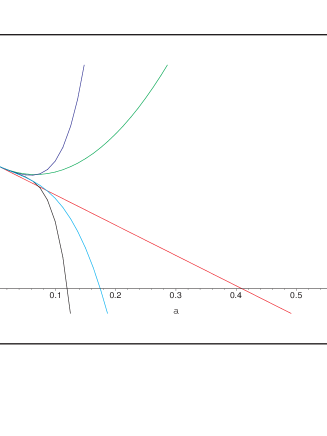
Figure 1: Plot of the ratio $R_{n}\equiv R_{a,n}$ defined in Eq. (12), as a function of $a$, for $N=10$ and (i) $n=2$ (red), (ii) $n=3$ (green), (iii) $n=4$ (cyan), (iv) $n=5$ (blue), and (v) $n=6$ (black) (colors in online version). Along a counterclockwise path around the point $(a,R_{n})=(0,1)$ starting at the point $(a,R_{n})=(0.1,0)$, the curves are for $n=6$, $n=4$, $n=2$, $n=3$, and $n=5$.

It is not necessary to carry out specific searches for a UV in the beta function for large $N$, because in this regime we can apply a more general type of analysis. This was done in lam and showed the absence of a UV zero in the $\lambda|\vec{\phi}|^{4}$ theory for $N\gg 1$. As in lam , we define the limit

$$N\to\infty\ ,\ \ {\rm with}\ x(\mu)\equiv Na(\mu)\ {\rm a\ finite\ function\ of}\ \mu.$$ (28)

This is denoted as the LN limit, with the symbol $\lim_{LN}$. The two scheme-independent coefficients, $b_{1}$ and $b_{2}$, are both polynomials of degree 1 in $N$, and the higher-loop coefficients $b_{\ell}$ are polynomials of degree $\ell-1$ in $N$ gracey_largeN , as indicated in Eq. (15). Thus, one can write $b_{1}=b_{1,1}N+b_{1,0}$, where $b_{1,1}=1/3$ and $b_{1,0}=8/3$. We extract the leading-$N$ factors and define

$$\hat{b}_{\ell}=\lim_{LN}\frac{b_{\ell}}{N^{\ell-1}}\quad{\rm for}\ \ \ell\geq 2\ .$$ (29)

so that these $\hat{b}_{\ell}$ with $\ell\geq 2$ are finite in the large-$N$ limit. The explicit values of the $\hat{b}_{\ell}$ follow from the expressions for the $b_{\ell}$ and are

$$\hat{b}_{2}=-1\ ,$$ (30)

$$\hat{b}_{3}=\frac{11}{72}=0.152778\ ,$$ (31)

$$\hat{b}_{4}=\frac{5}{3888}=1.2860\times 10^{-3}\ ,$$ (32)

$$\hat{b}_{5}=\frac{13}{62208}-\frac{\zeta(3)}{432}=-(2.57356\times 10^{-3})\ ,$$ (33)

and

$$\hat{b}_{6} = \frac{29}{933120}+\frac{11}{19440}\zeta(3)-\frac{\zeta(4)}{2160}$$ (34)

$$= 2.10179\times 10^{-4}\ .$$ (36)

(where $\zeta(4)=\pi^{4}/90$.)

Since the LN limit is defined so that $x(\mu)$ is a finite function of $\mu$, the appropriate beta function that is finite in this limit is

$$\beta_{x} = \frac{dx}{dt}=\lim_{LN}N\beta_{a}$$ (37)

$$= x^{2}\bigg{[}b_{1,1}+\frac{1}{N}\sum_{\ell=2}^{\infty}\hat{b}_{\ell}\,x^{\ell-1}\bigg{]}\ .$$ (39)

The $n$-loop beta function in the LN limit, denoted $\beta_{x,n\ell}$, is defined via Eq. (39) with the upper limit on the sum being $\ell=n$ rather than $\ell=\infty$. From Eq. (39), is it clear that in the LN limit lam , for any given loop order $n$, $\beta_{x,n\ell}$ has no UV zero $x_{{}_{UV,n\ell}}$, since

$$\lim_{LN}\frac{1}{N}\sum_{\ell=2}^{n}\hat{b}_{\ell}\,x^{\ell-1}=0\ .$$ (40)

Hence, in the $N\to\infty$ limit, as $\mu$ increases, $x(\mu)$ increases, eventually exceeding the range of values where the perturbative $n$-loop expansion of $\beta_{x,n\ell}$ is reliable. This result in the LN limit agrees with our specific calculations up to the six-loop level for large finite values of $N$ as shown in Table 2. For example, for $N=10^{4}$ (chosen to be larger than $N_{b4z}$, $N_{b5z}$, and $N_{b6z}$), the three-loop, four-loop, and six-loop beta functions have no UV zero, and although the five-loop beta function $\beta_{a,5\ell}$ has a UV zero, at $a_{{}_{UV,5\ell}}=0.003460$, it is a factor of 100 smaller than the two-loop value, $a_{{}_{UV,2\ell}}=0.3334$. Thus, neither of the necessary criteria for a reliably calculable UV zero of the six-loop beta function is satisfied here.

IV Analysis With Padé Approximants

IV.1 General

In the search for a possible UV zero of the six-loop beta function of the O($N$) $\lambda|\vec{\phi}|^{4}$ theory, it is also instructive to calculate and analyze Padé approximants (PAs) to this function. Moreover, these approximants can be used to investigate the general analytic structure of the beta function. Since the zero in question would occur away from the origin in coupling-constant space, it is convenient to extract an overall prefactor of $b_{1}a^{2}$ and compute Padé approximants to the reduced beta function, $\beta_{a,n\ell,{\rm red.}}$ defined in Eq. (11). Our six-loop results on a possible UV zero for this O($N$) $\lambda|\vec{\phi}|^{4}$ theory extend our previous studies of Padé approximants to the beta function that were carried out up to the five-loop level for general $N$ in lam and up to the six-loop level for $N=1$ in lam2 .

For a function $f(a)$ satisfying $f(0)=1$, with a finite series expansion about $a=0$ given by $f(a)=1+\sum_{s=1}^{n-1}c_{s}a^{s}$, the $[p,q]$ Padé approximant is the rational function

$$[p,q]=\frac{\sum_{j=0}^{p}N_{j}a^{j}}{\sum_{k=0}^{q}D_{k}a^{k}}\ ,$$ (41)

with polynomials in the numerator and denominator of degree $p$ and $q$, respectively, where $p+q=n-1$ and $N_{0}=1=D_{0}$ pade . The coefficients $N_{j}$ with $j=1,...,p$ and $D_{k}$ with $k=1,...,q$ are determined by the $m$ coefficients $c_{1},...,c_{n-1}$, so that the Taylor series expansion of the $[p,q]$ Padé approximant about $a=0$ matches the corresponding expansion of $f(a)$ up to its maximal order, $O(a^{n-1})$. For our application, $f(a)=\beta_{a,n\ell,{\rm red.}}$ and $c_{s}=b_{s+1}/b_{1}$ for $1\leq s\leq n-1$.

We recall some general properties of these Padé approximants. The $[n-1,0]$ PA to $\beta_{a,n\ell,{\rm red.}}$ is this function itself, i.e.,

$$[n-1,0]=\beta_{a,n\ell,{\rm red.}}\ .$$ (42)

Since we have already analyzed the zeros of $\beta_{a,n\ell,{\rm red.}}$ above, we do not discuss the $[n-1,0]$ approximants here. Moreover, the $[0,n-1]$ PA approximant has no zeros and hence is not useful for investigating a possible UV zero in the beta function. Thus, for the purpose of investigating a possible UV zero in the beta function, we shall use the $[p,q]$ PAs with $p\neq 0$ in addition to the analysis that we have already carried out for $\beta_{a,n\ell,{\rm red.}}$.

In order for a zero of Padé approximant to $\beta_{a,n\ell,{\rm red.}}$ to be physically meaningful, (i) it must occur on the positive real $a$ axis, and (ii) calculations of Padé approximants to the (reduced) $n$-loop beta functions with different loop orders should yield approximately the same value for this zero. Furthermore, (iii) if the Padé approximant has a pole on the positive real $a$ axis, this pole must not occur closer to the origin than the zero. This is clear, since if there were such a pole, then as $\mu$ increases from small values in the IR to large values in the UV and $a(\mu)$ increases from the vicinity of the origin, it would approach the pole before it reached the zero. In order for a zero of a $[p,q]$ Padé approximant to be considered physically meaningful, one might also consider imposing a stricter condition, namely that this zero must occur within the disk in the complex $a$ plane in which the PA has a convergent Taylor series expansion. Since the radius of this disk is determined by the real pole or pair of complex-conjugate poles closest to the origin, this condition would be that, in addition to properties (i)-(iii), the zero must be closer to the origin than any pole(s), even if a pole occurs on the negative real axis or if the PA has complex-conjugate pairs of poles. However, we will not have to consider imposing this last condition, since the zeros of PAs that we find do not satisfy the first three conditions. It should also be noted that $[p,q]$ Padé approximants in which both $p$ and $q$ are nonzero may exhibit nearly or exactly coincident pairs of zeros and poles. This type of behavior typically occurs if one tries to approximate (from the series expansion) a function that has fewer than $p$ zeros and $q$ poles with a $[p,q]$ Padé approximant. As will be evident from our results below, a number of the higher-order Padé approximants that we compute exhibit poles and zeros at points that are quite close to each other. In this case, it is expected that one may ignore these zero-pole pairs; i.e., the approximant is indicating that the actual function does not have a zero or pole at the nearly coincident points.

As was noted above, the one-loop and two-loop coefficients in the beta function have the opposite sign, and for a large range of values of $N$, this sign alternation also holds for the higher-loop coefficients up to the highest-loop level to which they have been calculated, namely the six-loop level (in the $\overline{\rm MS}$ scheme). A function with a pole on the negative real axis could produce this type of sign alternation in a series expansion. For this reason, we will analyze the $[p,q]$ Padé approximants to $\beta_{a,n\ell,{\rm red.}}$ with $q\neq 0$ to investigate indications of a possible pole in this function on the negative $a$ axis.

The coefficients $N_{j}$ and $D_{k}$ in the $[p,q]$ Padé approximant (41) are, themselves, rational functions of the coefficients $b_{\ell}$ with $1\leq\ell\leq n$. For example, the three-loop reduced beta function is given by the $n=3$ special case of Eq. (11), namely $\beta_{a,3\ell,{\rm red.}}=1+(b_{2}/b_{1})a+(b_{3}/b_{1})a^{2}$, which is identical to the [2,0] PA. This function $\beta_{a,3\ell,{\rm red.}}$ has no physical zeros, but instead a complex-conjugate pair of zeros for all $N\geq 1$ lam . The [1,1] PA to this function is

$$[1,1]=\frac{1+\Big{(}\frac{b_{2}^{2}-b_{1}b_{3}}{b_{1}b_{2}}\Big{)}a}{1-\Big{(}\frac{b_{3}}{b_{2}}\Big{)}a}\ .$$ (43)

This [1,1] PA has no physical zeros lam ; the formal zero is given by

$$a_{[1,1]_{\rm zero}}=\frac{b_{1}b_{2}}{b_{1}b_{3}-b_{2}^{2}}=-\frac{72(N+8)(3N+14)}{33N^{3}+(538+480\zeta(3))N^{2}+(4288+5952\zeta(3))N+(9568+16896\zeta(3))}\ .$$ (44)

This is manifestly negative for all physical $N$. This [1,1] PA also has a pole at

$$a_{[1,1]_{\rm pole}}=\frac{b_{2}}{b_{3}}=-\frac{72(3N+14)}{33N^{2}+(922+480\zeta(3))N+(2960+2112\zeta(3))}\ ,$$ (45)

which is also clearly negative for all physical $N$. In passing, we note that the pole occurs closer to the origin than the zero, as is evident from the fact that the difference is a positive quantity:

$$a_{[1,1]_{\rm pole}}-a_{[1,1]_{\rm zero}}=\frac{b_{2}^{3}}{b_{3}(b_{2}^{2}-b_{1}b_{3})}$$ (46)

$$= \frac{5184(3N+14)^{3}}{\Big{[}33N^{2}+(922+480\zeta(3))N+(2960+2112\zeta(3))\Big{]}\Big{[}33N^{3}+(538+480\zeta(3))N^{2}+(4288+5952\zeta(3))N+(9568+16896\zeta(3))\Big{]}}\ .$$ (48)

The [0,2] Padé approximant to $\beta_{a,3\ell,{\rm red.}}$ is

$$[0,2]=\frac{1}{1-\Big{(}\frac{b_{2}}{b_{1}}\Big{)}\,a+\frac{(b_{2}^{2}-b_{1}b_{3})}{b_{1}^{2}}\,a^{2}}\ .$$ (51)

This approximant has poles at

$$a_{[0,2]_{\rm pole}}=\frac{b_{1}[b_{2}\pm\sqrt{4b_{1}b_{3}-3b_{2}^{2}}\ ]}{2(b_{2}^{2}-b_{1}b_{3})}\ .$$ (52)

Similar but progressively more complicated analytic expressions can be given for the higher-order $[p,q]$ Padé approximants in terms of the coefficients $b_{n}$ and explicitly as rational functions of $N$, but these are sufficient to illustrate the results.

IV.2 Analysis for Theory with $N=1$

We begin with the case $N=1$. The six-loop beta function for this case was calculated in kp1 and analyzed for a possible UV zero in lam2 . Numerically,

$$\beta_{a,6\ell} = a^{2}\Big{(}3-\frac{17}{3}a+32.5497a^{2}-271.6058a^{3}$$ (53)

$$+ 2848.568a^{4}-34776.131a^{5}\Big{)}\ .$$ (55)

The reduced six-loop beta function is thus

$$\beta_{a,6\ell,{\rm red.}} = 1-1.8888889a+10.8499a^{2}-90.53527a^{3}$$ (56)

$$+ 949.5227a^{4}-11592.044a^{5}\ .$$ (58)

The $[p,q]$ Padé approximants (with $p\neq 0$) to the $n$-loop beta functions with $3\leq n\leq 6$ were calculated and studied in lam2 . We recall these here. Since we are also investigating a possible pole on the negative real axis here, we calculate and analyze the $[0,q]$ Padé approximants. At the three-loop level, the $[p,q]$ Padé approximants for $\beta_{a,3\ell,{\rm red.}}$ (with $q\neq 0$) are

$$[1,1]=\frac{1+3.85517a}{1+5.74406a}$$ (59)

and

$$[0,2]=\frac{1}{1+1.88889a-7.28199a^{2}}\ .$$ (60)

At the four-loop level, the PAs for $\beta_{a,4\ell,{\rm red.}}$ are

$$[2,1]=\frac{1+6.45546a-4.91165a^{2}}{1+8.344345a}\ ,$$ (61)

$$[1,2]=\frac{1+7.72950a}{1+9.61839a+7.31817a^{2}}\ ,$$ (62)

and

$$[0,3]=\frac{1}{1+1.88889a-7.28199a^{2}+56.2861a^{3}}\ .$$ (63)

Proceeding to the five-loop level, the Padé approximants to $\beta_{a,5\ell,{\rm red.}}$ are

$$[3,1]=\frac{1+8.5989a-8.9605a^{2}+23.2571a^{3}}{1+10.4879a}\ ,$$ (64)

$$[2,2]=\frac{1+13.3341a+21.6066a^{2}}{1+15.2230a+39.51125a^{2}}\ ,$$ (65)

$$[1,3]=\frac{1+10.5387a}{1+12.4276a+12.6245a^{2}-20.4568a^{3}}\ ,$$ (66)

and

$$[0,4] = \frac{1}{1+1.88889a-7.28199a^{2}+56.2861a^{3}-593.1846a^{4}}\ .$$ (67)

Finally, at the six-loop level, the Padé approximants to $\beta_{a,6\ell,{\rm red.}}$ are

$$[4,1]=\frac{1+10.3193a-12.2102a^{2}+41.9233a^{3}-155.757a^{4}}{1+12.2083a}\ ,$$ (70)

$$[3,2]=\frac{1+17.0166a+45.3789a^{2}-18.0872a^{3}}{1+18.9055a+70.2394a^{2}}\ ,$$ (71)

$$[2,3]=\frac{1+17.8537a+56.5411a^{2}}{1+19.7426a+82.9828a^{2}+33.0754a^{3}}\ ,$$ (72)

$$[1,4] = \frac{1+12.48863a}{1+14.3775a+16.3076a^{2}-34.6560a^{3}+109.7524a^{4}}\$$ (73)

and

$$[0,5]=\frac{1}{1+1.88889a-7.28199a^{2}+56.2861a^{3}-593.1846a^{4}+7408.0652a^{5}}\ .$$ (76)

We list the real zeros and poles in these Padé approximants in Table 3. In order for these various $[p,q]$ Padé approximants to the reduced $n$-loop beta functions $\beta_{a,n\ell,{\rm red.}}$ to give evidence for a UV zero in the actual beta function, or equivalently, in $\beta_{a,{\rm red.}}=\beta_{a,\infty\ell,{\rm red.}}$, the ones with $p\neq 0$ would have to consistently feature a zero at approximately the same value of $a$. Clearly, they do not do this. Many of the approximants have no physical (real, positive) zero and for the the ones that do, the respective values are significantly different from each other. Furthermore, for the loop orders $n=2,4,6$ where the respective $n$-loop beta functions do exhibit UV zeros (namely $a_{{}_{UV,2\ell}}=0.5294$, $a_{{}_{UV,4\ell}}=0.2333$, and $a_{{}_{UV,6\ell}}=0.1604$), the corresponding sets of Padé approximants do not reproduce these zeros. This is automatic at the two-loop level, since the only PA other than $\beta_{a,2\ell,{\rm red.}}$ itself is [0,1], which has no zero. At the $n=4$ loop level, the [1,2] PA has no physical UV zero, and although the [2,1] has one physical zero, it occurs at $a=1.4543$, six times larger than the UV zero $a_{{}_{UV,4\ell}}$ in the four-loop beta function. Moreover, the perturbative expansion of the [2,1] PA only converges in the disk $|a|<0.1198$ whose radius is set by the position of its pole at $a=-0.1198$, and both the physical zero and the unphysical zero of this [2,1] PA lie outside this disk. Similarly, the unphysical zero of the [1,2] PA lies outside the radius of convergence of the Taylor series expansion of this PA, which is set by its unphysical pole at $a=-0.1138$. At the six-loop level, none of the Padé approximants exhibits a zero near to the UV zero in the six-loop beta function, at $a_{{}_{UV,6\ell}}=0.1604$.

Aside from the two-loop level, where the pole in the [0,1] PA always occurs at minus the value of the zero in the [1,0] PA, in each case where $p\neq 0$ so that a $[p,q]$ PA has one or more zeros, this approximant has a pole closer to the origin than the zero(s). Moreover, one can also observe many examples of nearly coincident zero-pole pairs. For example, at the six-loop level, the [4,1] PA has a zero at $a=-0.085$ and a pole at $a=-0.082$, the [3,2] PA has a zero at $a=-0.074$ and a pole at $a=-0.072$, and the [2,3] PA has a zero at $a=-0.073$ and a pole at $a=-0.072$, and so forth for other approximants (see Table 3 for values listed with more digits).

We may also use these Padé approximants to investigate the possible presence of a pole in the $n$-loop beta functions. As noted above, for a large range of values of $N$, the coefficients $b_{n}$ alternate in sign. In general, if the Taylor series expansion of a function $f(a)$ around $a=0$ has this property of alternating signs, it can indicate the influence of a pole on the negative $a$ axis. The $[p,q]$ Padé approximants with $q\neq 0$ thus provide a test for a possible pole in the beta function. In general, one would expect that if a pole were present in the full beta function, then for many values of $p$ and $q\neq 0$, the $[p,q]$ Padé approximant would feature a pole at approximately the position of the pole in this full beta function. However, these Padé approximants do not do this. Our results in Table 3 do not yield persuasive evidence for such a pole, although they do not exclude this possibility. In particular, although the [2,2] PA to $\beta_{a,5\ell,{\rm red.}}$ and the [1,4] PA to $\beta_{a,6\ell,{\rm red.}}$ both exhibit a pole at $a=-0.301$, this pole is not present in the other $[p,q]$ Padés to the $\beta_{a,n\ell,{\rm red.}}$ functions with $2\leq n\leq 6$. Furthermore, as was true with a number of the zeros in various Padé approximants, we find that many poles are members of nearly coincident zero-pole pairs, indicating that they are not likely to actually be present in the beta function.

Summarizing, our Padé analysis of the $N=1$ $\lambda\phi^{4}$ theory does not give robust evidence for a UV zero of the beta function. We have used it also to probe for a possible pole at negative $a$ in the beta function, and have not found compelling evidence of this either.

IV.3 Cases with Larger $N$

It is also valuable to carry out a corresponding calculation and analysis of Padé approximants for the (reduced) six-loop beta function of the $\lambda|\vec{\phi}|^{4}$ theory with higher values of $N$. We have performed this study. We show the resultant zeros and poles of Padé approximants for the illustrative value $N=10$ in Table 4. These are qualitatively similar to our results for the theory with $N=1$, and lead to the same conclusions. We find similar results for other values of $N$.

Thus, from our calculation and analysis of Padé approximants to the $n$-loop beta function up to the $n=6$ loop level, we add to the evidence that we obtained from the analysis of the zeros of $\beta_{a,n\ell,{\rm red.}}$ against a reliably calculable UV zero in the beta function of the $\lambda|\vec{\phi}|^{4}$ theory.

IV.4 Extensions

Here we have considered a the O($N$) $\lambda|\vec{\phi}|^{4}$ scalar field theory in isolation. This type of analysis complements studies of more complicated theories with scalar, fermion, and gauge fields and hence multiple (quartic, Yukawa, and gauge) couplings. The beta functions in the latter theories involve not only powers of single couplings, but also terms containing products of different couplings, and, understandably, have not been calculated in general to an order as high as six loops. The renormalization-group behavior of theories with scalar and fermion fields have been studied both perturbatively cel and nonperturbatively yuk . For fully nonperturbative analyses, the lattice formulation has provided a powerful tool. Recent studies using perturbatively calculated beta functions that have found RG fixed points include cp3 , motivating continued interest in the phenomenon of asymptotic safety in these multiple-coupling theories.

V Conclusions

In this work we have investigated whether the beta function for the O($N$) $\lambda|\vec{\phi}|^{4}$ theory in $d=4$ spacetime dimensions exhibits evidence for an ultraviolet zero, using the six-loop beta function recently calculated in kp . For the range of quartic coupling $\lambda$, or equivalently, $a=\lambda/(16\pi^{2})$, where a perturbative calculation is reliable, we do not find evidence for such a UV zero. This conclusion is in accord with, and extends, our five-loop analysis in lam for general $N$ and our six-loop analysis in lam2 for $N=1$. Our methods include both analysis of the zeros of the six-loop beta function itself and calculation and study of the zeros of Padé approximants. Our conclusion provides further support for the modern view of the O($N$) $\lambda|\vec{\phi}|^{4}$ theory as an effective field theory that is applicable only over a restricted range of momentum scales $\mu$. In view of the alternating nature of the series expansion for the beta function, we have also used Padé approximants to investigate possible indications for a pole in the beta function at negative $a$, but we have not found persuasive evidence for this.

Appendix A Beta Function Coefficients at Loop Orders $n=3,\ 4,\ 5$

In this appendix, for reference, we list the $n$-loop coefficients $b_{n}$ in the beta function (8) for $3\leq n\leq 5$, as calculated in the widely used $\overline{\rm MS}$ scheme. Numerical values of the equivalent coefficients $\bar{b}_{n}=b_{n}/(4\pi)^{n}$ are given in Table 1 for a relevant set of values of $N$.

The coefficient $b_{3}$ is bgz74 ; b345 ; kbook

$$b_{3} = \frac{11}{72}N^{2}+\bigg{(}\frac{461}{108}+\frac{20\zeta(3)}{9}\bigg{)}N+\frac{370}{27}+\frac{88\zeta(3)}{9}\ .$$ (77)

Numerically,

$$b_{3}=0.15278N^{2}+6.93976N+24.4571\ ,$$ (80)

to the indicated floating-point accuracy. Clearly, for all physical $N$, $b_{3}$ is positive and is a monotonically increasing function of $N$.

The four-loop coefficient is b345

$$b_{4} = \frac{5}{3888}N^{3}+\bigg{(}-\frac{395}{243}-\frac{14\zeta(3)}{9}+\frac{10\zeta(4)}{27}-\frac{80\zeta(5)}{81}\bigg{)}N^{2}+\bigg{(}-\frac{10057}{486}-\frac{1528\zeta(3)}{81}+\frac{124\zeta(4)}{27}-\frac{2200\zeta(5)}{81}\bigg{)}N$$ (81)

$$- \frac{24581}{486}-\frac{4664\zeta(3)}{81}+\frac{352\zeta(4)}{27}-\frac{2480\zeta(5)}{27}\ .$$ (83)

Numerically,

$$b_{4} = (1.2860\times 10^{-3})N^{3}-4.11865N^{2}-66.5621N$$ (84)

$$- 200.92637\ .$$ (86)

The coefficient $b_{5}$ is b345

$$b_{5} = \bigg{(}\frac{13}{62208}-\frac{\zeta(3)}{432}\bigg{)}N^{4}+\bigg{(}\frac{6289}{31104}+\frac{26\zeta(3)}{81}-\frac{2\zeta(3)^{2}}{27}-\frac{7\zeta(4)}{24}+\frac{305\zeta(5)}{243}-\frac{25\zeta(6)}{81}\bigg{)}N^{3}$$ (87)

$$+ \bigg{(}\frac{50531}{3888}+\frac{8455\zeta(3)}{486}-\frac{59\zeta(3)^{2}}{81}-\frac{347\zeta(4)}{54}+\frac{7466\zeta(5)}{243}-\frac{1775\zeta(6)}{243}+\frac{686\zeta(7)}{27}\bigg{)}N^{2}$$ (89)

$$+ \bigg{(}\frac{103849}{972}+\frac{69035\zeta(3)}{486}+\frac{446\zeta(3)^{2}}{81}-\frac{2383\zeta(4)}{54}+\frac{66986\zeta(5)}{243}-\frac{7825\zeta(6)}{81}+343\zeta(7)\bigg{)}N$$ (91)

$$+ \frac{17158}{81}+\frac{27382\zeta(3)}{81}+\frac{1088\zeta(3)^{2}}{27}-\frac{880\zeta(4)}{9}+\frac{55028\zeta(5)}{81}-\frac{6200\zeta(6)}{27}+\frac{25774\zeta(7)}{27}\ .$$ (93)

Numerically,

$$b_{5}=-(2.57356\times 10^{-3})N^{4}+1.152827N^{3}+72.23315N^{2}+771.20866N+2003.97619\ .$$ (94)

Appendix B Discriminants

The analysis of the zeros of $\beta_{a,n\ell}$ requires an analysis of the zeros of the equation (24), of degree $n-1$ in the variable $a$, given by Eq. (5). For this purpose, we use the discriminant. Given a polynomial equation of degree $m$ in the variable $a$, $P_{m}(a)=0$, where $P_{m}(a)=\sum_{s=0}^{m}c_{s}a^{s}$, we will label the $m$ roots as $P_{m}(a)=0$ as $\{a_{1},...,a_{m}\}$. The discriminant of this equation is disc

$$\Delta_{m}\equiv\Big{[}c_{m}^{m-1}\prod_{i<j}(a_{i}-a_{j})\Big{]}^{2}\ .$$ (95)

Since $\Delta_{m}$ is a symmetric polynomial in the roots of the equation $P_{m}(a)=0$, the symmetric function theorem shows that it can be written as a polynomial in the coefficients of $P_{m}(a)$ symfun , as indicated in the notation $\Delta_{m}(c_{0},...,c_{m})$. For our purposes in analyzing the roots of Eq. (24), we have

$$c_{s}=b_{s+1}$$ (96)

for $s=0,...,m$. Since Eq. (24) for the zeros of the $n$-loop beta function away from the origin is of degree $m=n-1$ in $a$, its discriminant is $\Delta_{n-1}(b_{1},b_{2},...,b_{n})$.

The discriminant $\Delta_{m}$ can be calculated in terms of the $(2m-1)\times(2m-1)$ Sylvester matrix of $P_{m}(a)$ and $P_{m}(a)^{\prime}=dP(a)/da$, proportional to the matrix $S_{P_{m},P_{m}^{\prime}}$ disc :

$$\Delta_{m}=(-1)^{m(m-1)/2}c_{m}^{-1}{\rm det}(S_{P_{m},P_{m}^{\prime}})\ .$$ (97)

The $m=2$ discriminant is well-known; $\Delta_{2}(c_{0},c_{1},c_{2})=c_{1}^{2}-4c_{0}c_{2}$.

For $\Delta_{3}$, the $S_{P_{3},P_{3}^{\prime}}$ matrix is

$$S_{P_{3},P_{3}^{\prime}}=\left(\begin{array}[]{ccccc}c_{3}&c_{2}&c_{1}&c_{0}&0\\ 0&c_{3}&c_{2}&c_{1}&c_{0}\\ 3c_{3}&2c_{2}&c_{1}&0&0\\ 0&3c_{3}&2c_{2}&c_{1}&0\\ 0&0&3c_{3}&2c_{2}&c_{1}\end{array}\right)\ ,$$ (98)

yielding the discriminant

$$\Delta_{3}(c_{0},c_{1},c_{2},c_{3}) = c_{1}^{2}c_{2}^{2}-27c_{0}^{2}c_{3}^{2}-4(c_{0}c_{2}^{3}+c_{3}c_{1}^{3})$$ (99)

$$+ 18c_{0}c_{1}c_{2}c_{3}\ .$$ (101)

For $\Delta_{4}$ and $\Delta_{5}$, the relevant $S_{P_{m},P_{m}^{\prime}}$ matrices are

$$S_{P_{4},P_{4}^{\prime}}=\left(\begin{array}[]{ccccccc}c_{4}&c_{3}&c_{2}&c_{1}&c_{0}&0&0\\ 0&c_{4}&c_{3}&c_{2}&c_{1}&c_{0}&0\\ 0&0&c_{4}&c_{3}&c_{2}&c_{1}&c_{0}\\ 4c_{4}&3c_{3}&2c_{2}&c_{1}&0&0&0\\ 0&4c_{4}&3c_{3}&2c_{2}&c_{1}&0&0\\ 0&0&4c_{4}&3c_{3}&2c_{2}&c_{1}&0\\ 0&0&0&4c_{4}&3c_{3}&2c_{2}&c_{1}\end{array}\right)$$ (102)

and

$$S_{P_{5},P_{5}^{\prime}}=\left(\begin{array}[]{ccccccccc}c_{5}&c_{4}&c_{3}&c_{2}&c_{1}&c_{0}&0&0&0\\ 0&c_{5}&c_{4}&c_{3}&c_{2}&c_{1}&c_{0}&0&0\\ 0&0&c_{5}&c_{4}&c_{3}&c_{2}&c_{1}&c_{0}&0\\ 5c_{5}&4c_{4}&3c_{3}&2c_{2}&c_{1}&0&0&0&0\\ 0&5c_{5}&4c_{4}&3c_{3}&2c_{2}&c_{1}&0&0&0\\ 0&0&5c_{5}&4c_{4}&3c_{3}&2c_{2}&c_{1}&0&0\\ 0&0&0&5c_{5}&4c_{4}&3c_{3}&2c_{2}&c_{1}&0\\ 0&0&0&0&5c_{5}&4c_{4}&3c_{3}&2c_{2}&c_{1}\end{array}\right)$$ (103)

From these matrices we calculate the corresponding discriminants according to Eq. (97) with (96). At the $n$-loop level, the relevant equation for a UV zero is Eq. (24), of degree $n-1$ in $a$. It follows from Eqs. (96) and (97) that the disciminant for this Eq. (24), namely $\Delta_{n-1}(b_{1},...,b_{n})$, is a homogeneous polynomial of degree $2(n-2)$ in the beta function coefficients $b_{\ell}$, $1\leq\ell\leq n$, i.e.,

$${\rm deg}_{\{b_{\ell}\}}[\Delta_{n-1}(b_{1},...,b_{n})]=2(n-2)\ .$$ (104)

This is illustrated at the $n=3$ loop level, by $\Delta_{2}(b_{1},b_{2},b_{3})=b_{1}^{2}-4b_{1}b_{3}$, at the $n=4$ loop level by

$$\Delta_{3}(b_{1},b_{2},b_{3},b_{4}) = b_{2}^{2}b_{3}^{2}-27b_{1}^{2}b_{4}^{2}-4(b_{1}b_{3}^{3}+b_{4}b_{2}^{3})$$ (105)

$$+ 18b_{1}b_{2}b_{3}b_{4}$$ (107)

and so forth for higher loop order $n$.

Appendix C Illustrative Function and Analysis

As an illustration of the effectiveness of Padé approximants in testing for indications of zeros and poles in a function based on information from its Taylor series expansion, in this appendix we construct and analyze a test function using these approximants. Thus, let us consider the rational function

$$f(a)=\frac{1+ra}{1+sa}\ ,$$ (108)

where $r$ and $s$ are real constants with $s>0$ and $r\geq 0$. This function has a zero at $a=-1/r$ and a pole at $a=-1/s$. It has the Taylor series expansion about $a=0$

$$f(a)=1+(r-s)\sum_{k=1}^{\infty}(-1)^{k-1}s^{k-1}a^{k}\ .$$ (109)

As is evident from Eq. (109), given that $s>0$, the coefficients of the $a^{k}$ terms in the sum $\sum_{k=1}^{\infty}(-1)^{k-1}s^{k-1}a^{k}$ alternate in sign. This property holds, independent of whether $r$ is zero or nonzero and, in the latter case, independent of the sign of $r$. The additional condition that $s>r$ guarantees that the $O(a)$ term is opposite in sign from the constant term, and hence that the full series is alternating in sign. The resultant alternating-sign property of the terms in the Taylor series (109) reproduces the alternating-sign property of the Taylor series expansion of $\beta_{a,{\rm red.}}$ which holds for a large range of values of $N$, namely $1\leq N\leq 504$. Recall that all of the Padé approximants that we have calculated for $\beta_{a,n\ell,{\rm red.}}$ up to $n=6$ loop order that have $p\neq 0$ and hence have zeros, also have the property that they contain a pole closer to the origin than the zero of minimal magnitude. This property is incorporated in the test function (108), since we take $s>r$. Then $f(a)=1-(s-r)a[1-sa+(sa)^{2}-(sa)^{3}+...]$.

As was discussed in the text, one of the purposes of our analysis with Padé approximants was to test for a stable zero and/or pole in $\beta_{a,{\rm red.}}$. This Padé method has the capability of doing this, as is evident from the fact that when one calculates $[p,q]$ Padé approximants to the series (109) with $p\geq 1$ and $q\geq 1$, they successfully identify the exact function, $f(a)$, given in (108).

Table 1: Values of the $\bar{b}_{\ell}$ coefficients for $1\leq\ell\leq 6$ as functions of $N$ for $1\leq N\leq 10$ and illustrative larger values of $N$. Notation $a$  e  $n$ means $a\times 10^{n}$.

$N$	$\bar{b}_{1}$	$\bar{b}_{2}$	$\bar{b}_{3}$	$\bar{b}_{4}$	$\bar{b}_{5}$	$\bar{b}_{6}$
1	0.2387	$-0.03588$	0.01640	$-0.01089$	0.09090	$-0.008831$
2	0.2653	$-0.04222$	0.02013	$-0.01406$	0.01227	$-0.012443$
3	0.2918	$-0.04855$	0.02401	$-0.01755$	0.01595	$-0.016822$
4	0.3183	$-0.05488$	0.02805	$-0.02137$	0.02016	$-0.022035$
5	0.3448	$-0.06121$	0.03224	$-0.02553$	0.02492	$-0.028147$
6	0.3714	$-0.06755$	0.03658	$-0.03001$	0.03024	$-0.035229$
7	0.3979	$-0.07388$	0.04108	$-0.03482$	0.03616	$-0.043347$
8	0.4244	$-0.08021$	0.04573	$-0.03996$	0.04269	$-0.052571$
9	0.4509	$-0.08655$	0.05054	$-0.04542$	0.04984	$-0.062971$
10	0.4775	$-0.09288$	0.05550	$-0.05121$	0.05765	$-0.074616$
30	1.00798	$-0.21953$	0.18703	$-0.23539$	0.38036	$-0.682937$
100	2.8648	$-0.6628$	1.1324	$-1.87505$	5.4152	$-16.57724$
200	5.5174	$-1.2961$	3.7918	$-6.7359$	26.0096	$-1.28518$e2
300	8.1700	$-1.9293$	7.9910	$-14.2812$	54.2973	$-4.24105$e2
400	10.8225	$-2.5626$	13.7300	$-24.2014$	63.0752	$-0.932587$e3
500	13.4751	$-3.1958$	21.0087	$-36.1873$	5.42998	$-1.560139$e3
600	16.1277	$-3.8291$	29.8273	$-49.9293$	$-1.85262$e2	$-2.02581$e3
700	18.7803	$-4.4624$	40.1856	$-65.1180$	$-5.95335$e2	$-1.79749$e3
800	21.4329	$-5.0956$	52.0837	$-81.4440$	$-1.33083$e3	$-27.8255$
900	24.0854	$-5.7289$	65.5216	$-98.5980$	$-2.51752$e3	4.50979e3
1.0e3	26.7380	$-6.3621$	80.4992	$-1.16270$e2	$-4.30084$e3	1.34853e4
2.0e3	53.2639	$-12.6947$	3.149645e2	$-2.53435$e2	$-1.01045$e5	1.15991e6
3.0e3	79.7897	$-19.0273$	7.03408e2	$-1.02078$e2	$-5.63816$e5	1.03446e7
4.0e3	1.063155e2	$-25.3598$	1.24583e3	6.472275e2	$-1.86330$e6	4.65918e7

Table 2: Values of the UV zero $a_{{}_{UV,n\ell}}$ of the $n$-loop beta function, $\beta_{\lambda,n\ell}$, for $n=2,...,6$, as a function of $N$, with $b_{n}$ calculated in the $\overline{\rm MS}$ scheme for $3\leq n\leq 6$. The notation “u” means that $\beta_{\lambda,n\ell}$ has only unphysical (complex and/or negative) zeros for $a\neq 0$.

$N$	$a_{{}_{UV,2\ell}}$	$a_{{}_{UV,3\ell}}$	$a_{{}_{UV,4\ell}}$	$a_{{}_{UV,5\ell}}$	$a_{{}_{UV,6\ell}}$
1	0.5294	u	0.2333	u	0.1604
2	0.5000	u	0.2217	u	0.1529
3	0.4783	u	0.2123	u	0.1467
4	0.4615	u	0.2044	u	0.1414
5	0.4483	u	0.1978	u	0.1368
6	0.4375	u	0.1920	u	0.1328
7	0.4286	u	0.1869	u	0.1292
8	0.42105	u	0.1823	u	0.1259
9	0.4146	u	0.1783	u	0.1229
10	0.4091	u	0.1746	u	0.1202
30	0.3654	u	0.1362	u	0.09033
100	0.3439	u	0.1012	u	0.05965
300	0.3370	u	0.07944	u	0.03783
500	0.3355	u	0.07341	0.08045	0.03074
800	0.3347	u	0.07137	0.02871	0.02866
890	0.3346	u	0.07164	0.02559	0.03829
900	0.3346	u	0.07170	0.02530	u
1000	0.3344	u	0.07241	0.02276	u
2000	0.3339	u	0.1054	0.01231	u
3000	0.3337	u	0.5475	0.008850	u
4000	0.3336	u	u	0.007042	u
$10^{4}$	0.3334	u	u	0.003460	u

Table 3: Values of real zeros and poles in the $[p,q]$ Padé approximants to the $n$-loop reduced beta function, $\beta_{a,n\ell,{\rm red.}}$ for $2\leq n\leq 6$ and $N=1$, with $b_{n}$, $3\leq n\leq 6$, calculated in the $\overline{\rm MS}$ scheme. Note that the $[n-1,0]$ Padé approximant is the function $\beta_{a,n\ell,{\rm red.}}$ itself, whose zeros are given in Table 2. The symbol “na” means “not applicable”, and the symbols “ccp” and $k(ccp)$ mean a complex-conjugate pair of values and $k$ complex-conjugate pairs of values, respectively.

$n$	$[p,q]$	zeros	poles
2	[0,1]	na	$-0.5294$
3	[1,1]	$-0.2594$	$-0.1741$
3	[0,2]	na	$-0.2629$,  $0.5223$
4	[2,1]	$-0.1400$,  $1.4543$	$-0.1198$
4	[1,2]	$-0.1294$	$-0.1138$, $-1.2005$
4	[0,3]	na	$-0.1893$,  ccp
5	[3,1]	$-0.1024$,  ccp	$-0.09535$
5	[2,2]	$-0.08736$,  $-0.5298$	$-0.08401$,  $-0.3013$
5	[1,3]	$-0.09489$	$-0.08986$,  $-0.4644$,  1.1714
5	[0,4]	na	$-0.1538$,  0.2334,  ccp
6	[4,1]	$-0.085055$,  0.4675,  ccp	$-0.08191$
6	[3,2]	$-0.07366$,  $-0.2637$,  2.8463	$-0.07233$,  $-0.1968$
6	[2,3]	$-0.07279$,  $-0.2430$	$-0.07156$,  $-0.1878$,  $-2.2495$
6	[1,4]	$-0.08007$	$-0.07784$,  $-0.3012$,  ccp
6	[0,5]	na	$-0.1327$,  2(ccp)

Table 4: Values of real zeros and poles in the $[p,q]$ Padé approximants to the $n$-loop reduced beta function, $\beta_{a,n\ell,{\rm red.}}$ for $2\leq n\leq 6$ and $N=10$, with $b_{n}$, $3\leq n\leq 6$, calculated in the $\overline{\rm MS}$ scheme. Note that the $[n-1,0]$ Padé approximant is the function $\beta_{a,n\ell,{\rm red.}}$ itself, whose zeros are given in Table 2. The notation is the same as in Table 3.

$n$	$[p,q]$	zeros	poles
2	[0,1]	na	$-4091$
3	[1,1]	$-0.1974$	$-0.1332$
3	[0,2]	na	$-0.2021$,  $0.3996$
4	[2,1]	$-0.09864$,  1.01465	$-0.08623$
4	[1,2]	$-0.08989$	$-0.0808$,  $-0.8352$
4	[0,3]	na	$-0.1426$,  ccp
5	[3,1]	$-0.07576$,  ccp	$-0.07069$
5	[2,2]	$-0.06870$,  $-0.5462$	$-0.06547$,  $-0.2812$
5	[1,3]	$-0.071475$	$-0.06757$,  $-0.3892$,  1.0716
5	[0,4]	na	$-0.1154$,  0.1743,  ccp
6	[4,1]	$-0.06388$,  0.3526,  ccp	$-0.06149$
6	[3,2]	$-0.05486$,  $-0.1701$,  1.5187	$-0.05391$,  $-0.1362$
6	[2,3]	$-0.05259$,  $-0.1412$	$-0.05188$,  $-0.1194$,  $-1.1224$
6	[1,4]	$-0.06071$	$-0.05892$,  $-0.2352$,  ccp
6	[0,5]	na	$-0.0099505$,  2(ccp)

References

- (1) Some early studies on the renormalization group include E. C. G. Stueckelberg and A. Peterman, Helv. Phys. Acta 26, 499 (1953); M. Gell-Mann and F. Low, Phys. Rev. 95, 1300 (1954); N. N. Bogolubov and D. V. Shirkov, Doklad. Akad. Nauk SSSR 103, 391 (1955); C. G. Callan, Phys. Rev. D 2, 1541 (1970); K. Symanzik, Commun. Math. Phys. 18, 227 (1970); K. Wilson, Phys. Rev. D 3, 1818 (1971).
- (2) K. G. Wilson and J. Kogut, Phys. Repts. 12, 75 (1974); M. Aizenman, Commun. Math. Phys. 82, 69 (1982); B. Freedman, P. Smolensky, and D. Weingarten, Phys. Lett. B 113, 491 (1982); J. Fröhlich, Nucl. Phys. B 200, 281 (1982); R. F. Dashen and H. Neuberger, Phys. Rev. Lett. 50, 1897 (1983); M. Aizenman and R. Graham, Nucl. Phys. B 225, 261 (1983); C. B. Lang, Nucl. Phys. B 240, 577 (1984); J. Kuti, L. Lin, and Y. Shen, Phys. Rev. Lett. 61, 678 (1988); M. Lüscher and P. Weisz, Nucl. Phys. B 290, 25 (1987); M. Lüscher and P. Weisz, Nucl. Phys. B 318, 705 (1989); D. J. E. Callaway, Phys. Repts. 167, 241 (1988), and references therein.
- (3) S. Weinberg, The Quantum Theory of Fields (Cambridge Univ. Press, Cambridge, 1996), vol. II, ch. 18.
- (4) J. Zinn-Justin, Quantum Field Theory and Critical Phenomena, 4th ed. (Oxford Univ. Press, Oxford, 2002).
- (5) H. Kleinert and V. Schulte-Frohlinde, Critical Properties of Theories (World Scientific, Singapore, 2001).
- (6) R. Shrock, Phys. Rev. D 90, 065023 (2014) [arXiv:1408.3141].
- (7) R. Shrock, Phys. Rev. D 94, 125026 (2016) [arXiv:1610.03733].
- (8) M. V. Kompaniets and E. Panzer, PoS (Loops and Legs 2016 Conf.) 038 [arXiv:1606.09210].
- (9) M. V. Kompaniets and E. Panzer, arXiv:1705.06483. Taking account of the change from Minkowski to Euclidean metrics, our in Eq. (5) is equal to the coupling defined in this paper.
- (10) W. A. Bardeen, B. W. Lee, and R. E. Shrock, Phys. Rev. D 14, 985 (1976); E. Brézin and J. Zinn-Justin, Phys. Rev. B 14, 3110 (1976); see also A. Polyakov, Phys. Lett. B 59, 79 (1975).
- (11) E. Brézin, J. C. Le Guillou, and J. Zinn-Justin, Phys. Rev. D 9, 1121 (1974).
- (12) D. J. Gross, in R. Balian and J. Zinn-Justin, eds. Methods in Field Theory, Les Houches 1975 (North Holland, Amsterdam, 1976), p. 141.
- (13) W. A. Bardeen, A. J. Buras, D. W. Duke, and T. Muta, Phys. Rev. D 18, 3998 (1978). See also G. ’t Hooft, Nucl. Phys. B 61, 455 (1973).
- (14) J. Gracey, in Proc. of the 5th International Workshop AIHENP (Artificial Intelligence for High-Energy and Nuclear Physics) 1996, Nucl. Instr. Meth. A 389, 361 (1997), hep-ph/9609409.
- (15) H. Kleinert, J. Neu, V. Schulte-Frohlinde, K. G. Chetyrkin, and S. A. Larin, Phys. Lett. B 272, 39 (1991); Erratum: Phys. Lett. B 319, 545 (1993).
- (16) Here and below, when expressions are given for that evaluate to non-integral real values, it is understood that they are formal and are interpreted via an analytic continuation of from physical nonnegative integer values to real numbers.
- (17) L. N. Lipatov, Sov. Phys. JETP 45, 216 (1977) [Zh. Eksp. Teor. Fiz. 72, 411 (1977)]; E. Brézin, J. C. Le Guillou, and J. Zinn-Justin, Phys. Rev. D 15, 1544 (1977); G. Parisi, Phys. Lett. B 66, 167 (1977); M. C. Bergère and F. David, Phys. Lett. B 135, 412 (1984); J. C. Le Guillou and J. Zinn-Justin, eds., Large Order Behavior of Perturbation Theory (North-Holland, Amsterdam, 1990).
- (18) I. M. Gelfand, M. M. Kapranov, and A. V. Zelevinsky, Discriminants, Resultants, and Multidimensional Determinants (Birkhäuser, Boston, 1994).
- (19) T. A. Ryttov and R. Shrock, Phys. Rev. D 86, 065032 (2012); T. A. Ryttov and R. Shrock, Phys. Rev. D 86, 085005 (2012).
- (20) R. Shrock, Phys. Rev. D 88, 036003 (2013); Phys. Rev. D 90, 045011 (2014).
- (21) G. A. Baker, Essentials of Padé Approximants (Academic Press, New York, 1975).
- (22) Two early studies include T. P. Cheng, E. Eichten, and L.-F. Li, Phys. Rev. D 9, 2259 (1974); L. Maiani, G. Parisi and R. Petronzio, Nucl. Phys. B 136, 115 (1978).
- (23) Some early lattice studies of scalar-fermion theories include I-H. Lee and R. E. Shrock, Phys. Rev. Lett. 59, 14 (1987); I-H. Lee, J. Shigemitsu, and R. E. Shrock, Nucl. Phys. B 330, 225 (1990); Nucl. Phys. B 334, 265 (1990). A. Hasenfratz, W.-Q. Liu, and T. Neuhaus, Phys. Lett. B 236, 339 (1990); J. Shigemitsu, Nucl. Phys. Proc. Suppl. 20, 515 (1991); R. E. Shrock, in Quantum Fields on the Computer, ed. M. Creutz (World Scientific, Singapore, 1992), pp. 150-210.
- (24) Some recent studies include B. Grinstein and P. Uttayarat, JHEP 1107, 038 (2011); O. Antipin, M. Gillioz, E. Mølgaard, and F. Sannino, Phys. Rev. D 87, 125017 (2013); E. Mølgaard and R. Shrock, Phys. Rev. D 89, 105007 (2014); D. F. Litim, M. Mojaza, F. Sannino, JHEP 1601 (2016) 081; O. Akerlund and Ph. de Forcrand, Phys. Rev. D 93, 035015 (2016); F. F. Hansen, T. Janowski, K. Langaeble, R. B. Mann, F. Sannino, T. G. Steele, and Z.-W. Wang, arXiv:1706.06402 and references therein.
- (25) J. V. Uspensky, Theory of Equations (McGraw-Hill, New York, 1948);