Second-order Bounds of Gaussian Kernel-based Functions and its Application to
Nonlinear Optimal Control with Stability

Abstract

Guaranteeing stability of a designed control system is a challenging problem in data-driven control approaches such as Gaussian process (GP)-based control. The reason is that the inequality conditions, which are used in ensuring the stability, should be evaluated for all states in the state space, meaning that an infinite number of inequalities must be evaluated. Previous research introduced the idea of using a finite number of sampled states with the bounds of the stability inequalities near the samples. However, high-order bounds with respect to the distance between the samples are essential to decrease the number of sampling. From the standpoint of control theory, the requirement is not only evaluating stability but also simultaneously designing a controller. This paper overcomes theses two issues to stabilize GP-based dynamical systems. Second-order bounds of the stability inequalities are derived whereas existing approaches use first-order bounds. The proposed method obtaining the bounds are widely applicable to various functions such as polynomials, Gaussian processes, Gaussian mixture models, and sum/product functions of them. Unifying the derived bounds and nonlinear optimal control theory yields a stabilizing (sub-)optimal controller for GP dynamics. A numerical simulation demonstrates the stability performance of the proposed approach.

1 Introduction

A data-driven approach in the design of control law is a timely topic of considerable interest in machine-learning communities. Trending are Gaussian Process (GP) based methods [9, 20, 23] which have the capability to identify complex nonlinear dynamics with almost no prior knowledge of the underlying systems [22, 11]. In the systems identified by this promising technique, some control methods have been proposed based on model predictive control (MPC) [16], explicit MPC [13], and the iterative linear quadratic regulator [6]. Successful applications can be found in robotics [5, 9, 10], aircraft [14], and various artificial systems [8, 20].

A major concerns in control theory is the lack of “stability guarantee”. Many papers discussing GP-based control focus on results of the performance evaluations. This is clearly important; however, one should ascertain if the obtained control law might give unexpected results. Lack of stability could cause a critical situation. This work addresses this fundamental problem. We develop a framework guaranteeing stability. An advantage of this proposed method is that no specific control law is required before the GP-based identification. Other notable research efforts have tried to solve this stability problem, but by assuming a pre-defined control law (see below for details). Because of this advantage, for GP systems, the controller which realizes one of the classical and most important control schemes, optimal control, is also presented in this work.

Related works. Guaranteeing the stability of GP-based (nonlinear) dynamics is a challenging problem because stability conditions should be addressed throughout all of the state space, meaning that an infinite number of states must be evaluated. For the GP model with Gaussian kernels, stability has been guaranteed in the sense that any control results are included in a bounded state space [2, 3]. This result ensures that the system behavior does not diverge. However, convergence to a fixed point like equilibrium is not guaranteed.

An interesting idea recently introduced considers the infinite number of states by using a finite number of sampled states [15, 4, 23]. An illustrative sketch of the idea is provided in Fig.3 of [23]. Convergence to the equilibrium point is evaluated using several inequalities: the dynamics convergence rate [23], the Lyapunov inequality [4], and the linear matrix inequalities [15]. The bounds of the inequalities for all states near the sampled states are derived, using Lipschitz continuity as an example.

The above frontier works provide a path to guaranteeing stability. However, such bounds have a first order $O(\tau)$ of $\tau$, which means that the bound approaches to its true value with the order of the distance $\tau$ between the sampled states [15, 4]. For small $\tau$, many sampled states are required to describe the whole region of state space. This clearly results in a significant increase in computational complexity to evaluate the stability of the space.

Another major problem is that previous studies assume a pre-defined controller [2, 3, 4, 23]. From the control-theory point of view, building a stabilizing control law is of fundamental importance. The previous works do not answer the basic question: "How can we obtain a stabilizing control law for GP systems?".

Contributions. For the above-mentioned problems, this work provides a powerful theory in which, given a GP based system, its stability can be evaluated with modest computational complexity, and a stabilizing control law can also be obtained. To achieve the complexity reduction, we introduce the continuous piecewise affine (CPA) methods [12], which achieve the bounds with $O(\tau^{2})$. Unlike the existing CPA methods [18, 1], our method derives the $O(\tau^{2})$ bounds explicitly for the fundamental form of the Gaussian kernel based functions $\Phi:\mathbb{S}_{x}\rightarrow\mathbb{R}$, which is the linear combination of the basis function $\Phi_{j}:\mathbb{S}_{x}\rightarrow\mathbb{R}$ with the constants $c_{j}\in\mathbb{R}$

$$\exists\Phi^{\mathrm{L}},\Phi^{\mathrm{U}},\qquad\Phi^{\mathrm{L}}\leq\Phi(x):=\sum_{j=1}^{M}c_{j}\Phi_{j}(x)\leq\Phi^{\mathrm{U}},\qquad\Phi_{j}(x):=\prod_{k=1}^{N_{j}}\phi_{j,k}(x),$$ (1)

where $\phi_{j,k}:\mathbb{S}_{x}\rightarrow\mathbb{R}$, $M>0$, $N_{j}>0$, and $x\in\mathbb{S}_{x}$ is the state. The set $\mathbb{S}_{x}\subset\mathbb{R}^{n}$ is a sum set of $n$-simplexes. Suppose that $\phi_{j,k}(x)$ is a linear function of $x$ or the Gaussian kernel $K^{(i)}(x)$ (which will be exactly defined in (5) below). In this sense, this function is often observed in the control of the GP-based model. Of note is that the class of $\Phi(x)$ includes various types of flexible functions such as polynomials, Gaussian processes (means and variances), Gaussian mixture models, and sum/product functions of them. Because $\Phi(x)$ can be non-convex in $x$, it is difficult to find lower and upper bounds $\Phi^{\mathrm{L}}$,$\Phi^{\mathrm{U}}$ in general. The bounds of $\Phi(x)$ are efficient for evaluating inequality constraints for all $x\in\mathbb{S}_{x}$. In Sec. 3, we derive the second-order bounds of $\Phi(x)$.

There are only a few assumptions regarding the controller in the derivation of the bound with $O(\tau^{2})$. This is hugely advantageous because the stability of various controllers can be evaluated. This provides the framework for building GP system control laws. Let us consider a nonlinear system model that is affine with respect to its input:

$$\dot{x}(t) \;=\hat{f}(x(t))+\hat{g}(x(t))u(t),$$ (2)

where $x(t)\in\mathbb{R}^{n}$ and $u(t)\in\mathbb{R}^{m}$ are the state and control input at time $t$, respectively. Suppose all components of both the passive dynamics model $\hat{f}:\mathbb{R}^{n}\rightarrow\mathbb{R}^{n}$ and the control dynamics model $\hat{g}:\mathbb{R}^{n}\rightarrow\mathbb{R}^{n\times m}$ are included in the class of $\Phi(x)$. The actual dynamics $f(x)$ and $g(x)$ of unknown systems are identified as the GP models in (2). Let us assume that $f(x)$ and $g(x)$ are deterministic and $f(0)=0$.

The objective of this work is to control the system of (2) with stability. We focus on the following optimal control problem, in which the cost function $J(x(0),u)$ is minimized by the optimal control input $u_{*}$

$$u_{*}:=\operatornamewithlimits{\mathrm{arg~{}min}}_{u}J(u,x(0)),\quad J(u,x(0)):=\int_{0}^{\infty}\Big{\{}q(x(t))+\frac{1}{2}u(t)^{\mathrm{T}}R(x(t))u(t)\Big{\}}dt,$$ (3)

where the state cost $q:\mathbb{R}^{n}\rightarrow\mathbb{R}$ and control cost matrix $R:\mathbb{R}^{n}\rightarrow\mathbb{R}^{m\times m}$ are designed such that $q(x)$ is a positive definite function and $R(x)>0$ for all $x\in\mathbb{R}^{n}$. Suppose that $\mathbb{S}_{x}$ includes $x=0$. The goal is finding the (sub-)optimal control input which converges the state toward an equilibrium point ($x=0$). It is defined by asymptotic stability for a given region $\mathbb{S}_{x}$ as

$$\lim_{t\rightarrow\infty}x(t)=0,\;\forall x(0)\in\mathbb{S}_{x}.$$ (4)

In Sec. 4, a design method of a stabilizing (sub-)optimal controller is proposed to solve the above problem. The proposed method is based on nonlinear optimal control theory, specifically the Hamilton–Jacobi–Bellman (HJB) equation and the Lyapunov inequality. By employing a Gaussian kernel based parametric controller, the derived second-order bounds of $\Phi(x)$ can be applied to the stability analysis. A numerical simulation demonstrates the stability performance of the proposed approach in Sec. 5.

2 Preliminaries

Let $[v]_{i}$ be the $i$-th component of a vector $v\in\mathbb{R}^{n}$. For a matrix $A\in\mathbb{R}^{n\times m}$, $[A]_{i,j}\in\mathbb{R}$ is the component in the $i$-th row and $j$-th column, $[A]_{i,\cdot}\in\mathbb{R}^{m}$ is the $i$-th row vector, and $[A]_{\cdot,j}\in\mathbb{R}^{n}$ is the $j$-th column vector. For a symmetric matrix $A_{\mathrm{sym}}\in\mathbb{R}^{n\times n}$, $\lambda_{\mathrm{min}}(A_{\mathrm{sym}})$ and $\lambda_{\mathrm{max}}(A_{\mathrm{sym}})$ are the minimum and maximum eigenvalues of $A_{\mathrm{sym}}$.

Let us consider the Gaussian kernel function

$$K^{(i)}(x) :=\sigma_{f}\exp\Big{(}-\frac{1}{2}(x-x^{(i)})^{\mathrm{T}}\Sigma_{w}^{-1}(x-x^{(i)})\Big{)},$$ (5)

where $x^{(i)}\in\mathbb{S}_{x}$ is a data point of the state. The coefficient $\sigma_{f}>0\in\mathbb{R}$ and the positive definite matrix $\Sigma_{w}\in\mathbb{R}^{n\times n}$ are hyperparameters. The form of (5) is commonly used in various models such as kernel based linear models, Nadaraya-Watson models, and Gaussian processes. The following definitions are used in the main parts of this theory.

Definition 1 (Simplexes)

Given $\mathcal{N}=n+1$ sampled states $\tilde{x}_{k}\in\mathbb{S}_{x}$ $(k=1,2,...,\mathcal{N})$, which are affinely independent, let us define the distance $\tau$ and the state $\tilde{x}$ on the simplex $\mathbb{S}_{\tilde{x}}$ constructed by $\tilde{x}_{k}$

$$\tau :=\max_{k,l=1,2,...,\mathcal{N}}\|\tilde{x}_{k}-\tilde{x}_{l}\|/2,$$ (6)

$$\tilde{x}(s_{1},...,s_{\mathcal{N}}) :=\sum_{k=1}^{\mathcal{N}}s_{k}\tilde{x}_{k}\in\mathbb{S}_{\tilde{x}}:=\Big{\{}x\Big{|}x=\sum_{k=1}^{\mathcal{N}}s_{k}\tilde{x}_{k},\;\sum_{k=1}^{\mathcal{N}}s_{k}=1,\;s_{k}\geq 0,\;\forall k\Big{\}}.$$ (7)

Definition 2 (Linear interpolations)

For a continuous function $\xi:\mathbb{S}_{x}\rightarrow\mathbb{R}$, let us define a linear interpolation $\bar{\xi}:\mathbb{S}_{\tilde{x}}\rightarrow\mathbb{R}$ of $\xi(\tilde{x})$ on the simplex $\mathbb{S}_{\tilde{x}}$

$$\bar{\xi}(\tilde{x}(s_{1},...,s_{\mathcal{N}})):=\sum_{k=1}^{\mathcal{N}}s_{k}\xi(\tilde{x}_{k}).$$ (8)

Definition 3 (Lower and upper bounds $\epsilon(\tau,\mathbb{S}_{\tilde{x}})$)

For a continuous function $\xi:\mathbb{S}_{x}\rightarrow\mathbb{R}$, let us define a lower bound $-\epsilon_{\xi}^{\mathrm{L}}(\tau,\mathbb{S}_{\tilde{x}}){\leq 0}$ and an upper bound $\epsilon_{\xi}^{\mathrm{U}}(\tau,\mathbb{S}_{\tilde{x}}){\geq 0}$ of $\xi(\tilde{x})$ as

$$\forall\tilde{x}\in\mathbb{S}_{\tilde{x}},\quad-\epsilon_{\xi}^{\mathrm{L}}(\tau,\mathbb{S}_{\tilde{x}})\leq\xi(\tilde{x})-\bar{\xi}(\tilde{x})\leq\epsilon_{\xi}^{\mathrm{U}}(\tau,\mathbb{S}_{\tilde{x}}).$$ (9)

Remark

If $\xi(x)$ is constant or linear in $x$, $\epsilon_{\xi}^{\mathrm{L}}=\epsilon_{\xi}^{\mathrm{U}}=0$ holds.

3 Main results 1: second-order bounds of Gaussian kernel based functions

This section proposes a method which derives the bounds of the function $\Phi(x)$ in (1). We focus on the CPA methods with the linear interpolations [12, 18, 1]. In the framework of the CPA methods, the bounds $\epsilon_{\Phi}^{\mathrm{L}}(\tau,\mathbb{S}_{\tilde{x}})$ and $\epsilon_{\Phi}^{\mathrm{U}}(\tau,\mathbb{S}_{\tilde{x}})$ of $\Phi(x)$ (in Definition 3 above) are employed instead of the bounds $\Phi^{\mathrm{L}}$ and $\Phi^{\mathrm{U}}$. A function $\xi(x)$ is bounded on the simplex $\mathbb{S}_{\tilde{x}}$ as follows if $\epsilon_{\xi}^{\mathrm{L}}$ and $\epsilon_{\xi}^{\mathrm{U}}$ are obtained.

Lemma 1 (Bounding functions on the simplexes)

The following relation holds

$$\forall\tilde{x}\in\mathbb{S}_{\tilde{x}},\quad\min_{k}\xi(\tilde{x}_{k})-\epsilon_{\xi}^{\mathrm{L}}(\tau,\mathbb{S}_{\tilde{x}})\leq\xi(\tilde{x})\leq\max_{k}\xi(\tilde{x}_{k})+\epsilon_{\xi}^{\mathrm{U}}(\tau,\mathbb{S}_{\tilde{x}}).$$ (10)

Proof

Because $\sum_{k=1}^{\mathcal{N}}s_{k}=1$ and $s_{k}\geq 0$ for all $k$, $\min_{k}\xi(\tilde{x}_{k})\leq\bar{\xi}(\tilde{x})\leq\max_{k}\xi(\tilde{x}_{k})$ holds. Substituting this inequality into (9) yields (10). This completes the proof.

Remark

Let us define the simplex $\mathbb{S}_{\tilde{x},l}$ with the samples $\tilde{x}_{k,l}$ such that $\bigcup_{l}\mathbb{S}_{\tilde{x},l}=\mathbb{S}_{x}$. If the bounds $\epsilon_{\Phi}^{\mathrm{L}}(\tau,\mathbb{S}_{\tilde{x},l})$, $\epsilon_{\Phi}^{\mathrm{U}}(\tau,\mathbb{S}_{\tilde{x},l})$ are given for all $\mathbb{S}_{\tilde{x},l}$, the lower and upper bounds $\Phi^{\mathrm{L}}$ and $\Phi^{\mathrm{U}}$ of $\Phi(x)$ are obtained only by evaluating $\Phi(\tilde{x}_{k,l})$ for finite samples $\tilde{x}_{k,l}$

$$\Phi^{\mathrm{L}}=\min_{l}\{\min_{k}\Phi(\tilde{x}_{k,l})-\epsilon_{\Phi}^{\mathrm{L}}(\tau,\mathbb{S}_{\tilde{x},l})\}\leq\Phi(x)\leq\Phi^{\mathrm{U}}=\max_{l}\{\max_{k}\Phi(\tilde{x}_{k,l})+\epsilon_{\Phi}^{\mathrm{U}}(\tau,\mathbb{S}_{\tilde{x},l})\}.$$ (11)

On the basis of Lemma 1, the first contribution stated in Sec. 1 is obtained by finding the second-order bounds $\epsilon_{\Phi}^{\mathrm{L}}(\tau,\mathbb{S}_{\tilde{x}})$ and $\epsilon_{\Phi}^{\mathrm{U}}(\tau,\mathbb{S}_{\tilde{x}})$ of $\Phi(x)$. We derive the following two theorems to obtain the bounds. First, Theorem 1 derives the second-order bounds of the Gaussian kernels $K^{(i)}(x)$ included in the class $\phi_{j,k}(x)$. Thus, the bounds of $\phi_{j,k}(x)$, which is linear or $K^{(i)}(x)$, are $0$ or of $O(\tau^{2})$. Theorem 2 describes a general property of bounds of functions, which are sum of products of $\phi_{j,k}(x)$. Their bounds are explicitly derived as $O(\tau^{2})$. By iterating $\phi_{j,k}(x)$, a linear combination of the basis function $\Phi_{j}(x)$ is found, and the bound of $\Phi(x)$ in (1) is finally derived (see Remark in Theorem 2).

Theorem 1 (Second-order bounds of Gaussian kernels)

There exist lower and upper bounds $\epsilon_{K^{(i)}}^{\mathrm{L}}(\tau,\mathbb{S}_{\tilde{x}})$ and $\epsilon_{K^{(i)}}^{\mathrm{U}}(\tau,\mathbb{S}_{\tilde{x}})$ of the Gaussian kernels $K^{(i)}(\tilde{x})$ which are $O(\tau^{2})$ as follows

$$\forall\tilde{x}\in\mathbb{S}_{\tilde{x}},\quad \min_{k}K^{(i)}(\tilde{x}_{k})-\epsilon_{K^{(i)}}^{\mathrm{L}}(\tau,\mathbb{S}_{\tilde{x}})\leq K^{(i)}(\tilde{x})\leq\max_{k}K^{(i)}(\tilde{x}_{k})+\epsilon_{K^{(i)}}^{\mathrm{U}}(\tau,\mathbb{S}_{\tilde{x}}),$$ (12)

$$\epsilon_{K^{(i)}}^{\mathrm{L}}(\tau,\mathbb{S}_{\tilde{x}}) =\exp(-3/2)(\mathcal{N}-1)\sigma_{f}\lambda_{\mathrm{max}}(\Sigma_{w}^{-1})\tau^{2}=O(\tau^{2}),$$ (13)

$$\epsilon_{K^{(i)}}^{\mathrm{U}}(\tau,\mathbb{S}_{\tilde{x}}) =(\mathcal{N}-1)\sigma_{f}\lambda_{\mathrm{max}}(\Sigma_{w}^{-1})\tau^{2}/2=O(\tau^{2}).$$ (14)

Proof

The full proof is given in Appendix A.1.

The proof sketch. First, the case of $\mathcal{N}=2$ is considered. For a given $\hat{\tau}:=\|\tilde{x}_{1}-\tilde{x}_{2}\|/2\leq\tau$, $K^{(i)}(\tilde{x})$ on $\mathbb{S}_{\tilde{x}}$ can be expressed as the Gaussian function of a scalar variable $s_{1}\in[0,1]$

$$K^{(i)}(\tilde{x}(s_{1})) =\acute{\sigma}_{f}\exp(-\acute{\sigma}_{w}(2\hat{\tau}s_{1}-z^{(i)})^{2}),$$ (15)

where $z^{(i)}\in\mathbb{R}$, $\acute{\sigma}_{f}\leq\sigma_{f}$, and $\acute{\sigma}_{w}\leq\lambda_{\mathrm{max}}(\Sigma_{w}^{-1})/2$ are functions of $\tilde{x}_{1}$ and $\tilde{x}_{2}$.

Next, let us consider a $C^{2}$ function $\Psi:\mathbb{R}\rightarrow\mathbb{R}$ such that $\max_{y\in\mathbb{R}}|\Psi(y)|<\infty$, $-\infty<\min_{y\in\mathbb{R}}\partial\Psi(y)/\partial y<0$, $0<\max_{y\in\mathbb{R}}\partial\Psi(y)/\partial y<\infty$, and $\max_{y\in\mathbb{R}}|\partial^{2}\Psi(y)/\partial y^{2}|<\infty$ hold. For a given $s\in[0,1]$, $y_{1}\in\mathbb{R}$, $y_{2}:=y_{1}+2\hat{\tau}\in\mathbb{R}$, and $y(s):=sy_{1}+(1-s)y_{2}\in\mathbb{R}$, we extend the property with respect to the linear interpolation in [7] as follows

$$\frac{\hat{\tau}^{2}}{2}\min_{y\in\mathbb{R}}\Big{(}-\frac{\partial^{2}\Psi(\hat{y})}{\partial y^{2}}\Big{)}\leq\Psi(y(s))-\big{\{}s\Psi(y_{1})+(1-s)\Psi(y_{2})\big{\}}\leq\frac{\hat{\tau}^{2}}{2}\max_{y\in\mathbb{R}}\Big{(}-\frac{\partial^{2}\Psi(\hat{y})}{\partial y^{2}}\Big{)}.$$ (16)

Substituting $K^{(i)}(\tilde{x}(s))$ in (15) into $\Psi(y(s))$ derives the bounds in the case of $\mathcal{N}=2$

$$\epsilon_{K^{(i)}}^{\mathrm{L}}(\tau,\mathbb{S}_{\tilde{x}})|_{\mathcal{N}=2} =\exp(-3/2)\sigma_{f}\lambda_{\mathrm{max}}(\Sigma_{w}^{-1})\tau^{2},$$ (17)

$$\epsilon_{K^{(i)}}^{\mathrm{U}}(\tau,\mathbb{S}_{\tilde{x}})|_{\mathcal{N}=2} =\sigma_{f}\lambda_{\mathrm{max}}(\Sigma_{w}^{-1})\tau^{2}/2.$$ (18)

Finally, these results are extended. Multiplying (17) and (18) by $(\mathcal{N}-1)$ yields the bounds in the cases of $\mathcal{N}\geq 3$. This completes the proof.

Theorem 2 (Bounds of sums and products of functions)

For given Lipschitz continuous functions $\phi_{j}:\mathbb{S}_{x}\rightarrow\mathbb{R}$ and $\psi_{j}:\mathbb{S}_{x}\rightarrow\mathbb{R}$ $(i=1,2,...,\mathcal{M})$, suppose that $\epsilon_{\phi_{j}}^{\mathrm{L}}(\tau,\mathbb{S}_{\tilde{x}})$, $\epsilon_{\phi_{j}}^{\mathrm{U}}(\tau,\mathbb{S}_{\tilde{x}})$, $\epsilon_{\psi_{j}}^{\mathrm{L}}(\tau,\mathbb{S}_{\tilde{x}})$, and $\epsilon_{\psi_{j}}^{\mathrm{U}}(\tau,\mathbb{S}_{\tilde{x}})$ are explicitly given as $O(\tau^{2})$. Let us define a function $\chi:\mathbb{S}_{x}\rightarrow\mathbb{R}$ as

$$\chi(x) :=\sum_{j=1}^{\mathcal{M}}\phi_{j}(x)\psi_{j}(x),$$ (19)

$$\forall\tilde{x}\in\mathbb{S}_{\tilde{x}},\quad\min_{k}\chi(\tilde{x}_{k})-\epsilon_{\chi}^{\mathrm{L}}(\tau,\mathbb{S}_{\tilde{x}}) \leq\chi(\tilde{x})\leq\max_{k}\chi(\tilde{x}_{k})+\epsilon_{\chi}^{\mathrm{U}}(\tau,\mathbb{S}_{\tilde{x}}),$$ (20)

then the lower and upper bounds $\epsilon_{\chi}^{\mathrm{L}}(\tau,\mathbb{S}_{\tilde{x}})$ and $\epsilon_{\chi}^{\mathrm{U}}(\tau,\mathbb{S}_{\tilde{x}})$ of $\chi(\tilde{x})$ are given as explicit functions of $\tau$, $\phi_{j}(\tilde{x}_{k})$, $\psi_{j}(\tilde{x}_{k})$ $\epsilon_{\phi_{j}}^{\mathrm{L}}(\tau,\mathbb{S}_{\tilde{x}})$, $\epsilon_{\phi_{j}}^{\mathrm{U}}(\tau,\mathbb{S}_{\tilde{x}})$, $\epsilon_{\psi_{j}}^{\mathrm{L}}(\tau,\mathbb{S}_{\tilde{x}})$, and $\epsilon_{\psi_{j}}^{\mathrm{U}}(\tau,\mathbb{S}_{\tilde{x}})$ of $O(\tau^{2})$ (see the details (69) and (70) in Appendix A.2).

Proof

The full proof is given in Appendix A.2.

The proof sketch. We focus on $\phi_{j}(\tilde{x})\{\psi_{j}(\tilde{x})-\bar{\psi}_{j}(\tilde{x})\}$ and $\bar{\psi}_{j}(\tilde{x})\{\phi_{j}(\tilde{x})-\bar{\phi}_{j}(\tilde{x})\}$ and derive their bounds $\bar{\epsilon}$ which satisfy

$$-\bar{\epsilon}_{\psi_{j}}^{\mathrm{L}}(\tau,\mathbb{S}_{\tilde{x}},\phi_{j}(\tilde{x}))\leq\phi_{j}(\tilde{x})\{\psi_{j}(\tilde{x})-\bar{\psi}_{j}(\tilde{x})\}\leq\bar{\epsilon}_{\psi_{j}}^{\mathrm{U}}(\tau,\mathbb{S}_{\tilde{x}},\phi_{j}(\tilde{x})),$$ (21)

$$-\bar{\epsilon}_{\phi_{j}}^{\mathrm{L}}(\tau,\mathbb{S}_{\tilde{x}},\bar{\psi}_{j}(\tilde{x}))\leq\bar{\psi}_{j}(\tilde{x})\{\phi_{j}(\tilde{x})-\bar{\phi}_{j}(\tilde{x})\}\leq\bar{\epsilon}_{\phi_{j}}^{\mathrm{U}}(\tau,\mathbb{S}_{\tilde{x}},\bar{\psi}_{j}(\tilde{x})).$$ (22)

The relation between $\bar{\phi}_{j}(\tilde{x})\bar{\psi}_{j}(\tilde{x})$ and $\bar{\chi}(\tilde{x})$ is derived as

$$\mbox{$\sum_{j=1}^{\mathcal{M}}$}\bar{\phi}_{j}(\tilde{x})\bar{\psi}_{j}(\tilde{x})=\bar{\chi}(\tilde{x})+4\tau^{2}\mathcal{R}(s_{1},...,s_{\mathcal{N}}),$$ (23)

where $\mathcal{R}(s_{1},...,s_{\mathcal{N}})\in\mathbb{R}$ is a function of $(s_{1},...,s_{\mathcal{N}})$ which is bounded due to Lipschitz continuity of $\phi_{j}(\tilde{x})$ and $\psi_{j}(\tilde{x})$. Calculating the sum of (21) and (22) for all $j$ and substituting (23) yields

$$\chi(\tilde{x})-\bar{\chi}(\tilde{x})\leq\mbox{$\sum_{j=1}^{\mathcal{M}}$}\{\bar{\epsilon}_{\psi_{j}}^{\mathrm{U}}(\tau,\mathbb{S}_{\tilde{x}},\phi_{j}(\tilde{x}))+\bar{\epsilon}_{\phi_{j}}^{\mathrm{U}}(\tau,\mathbb{S}_{\tilde{x}},\bar{\psi}_{j}(\tilde{x}))\}+4\tau^{2}\mathcal{R}(s_{1},...,s_{\mathcal{N}}).$$ (24)

Here, the right hand side of (24) is still depended on $\tilde{x}$ and $(s_{1},...,s_{\mathcal{N}})$. By proving that the right hand side is a convex function, the its maximum is derived as the upper bound $\epsilon_{\chi}^{\mathrm{U}}(\tau,\mathbb{S}_{\tilde{x}})$ of $\chi(\tilde{x})$. The lower bound $\epsilon_{\chi}^{\mathrm{L}}(\tau,\mathbb{S}_{\tilde{x}})$ is derived in a similar manner. This completes the proof.

Remark

Based on Theorem 2, for a given $\Phi(x)$ in (1), the bounds $\epsilon_{\Phi}^{\mathrm{L}}(\tau,\mathbb{S}_{\tilde{x},l})$ and $\epsilon_{\Phi}^{\mathrm{U}}(\tau,\mathbb{S}_{\tilde{x},l})$ are derived for any set $\mathbb{S}_{\tilde{x},l}\subseteq\mathbb{S}_{x}$. For example, the following recurrence formula is defined

$$\psi_{j,k}(x) :=\prod_{a=1}^{k}\phi_{j,a}(x),\quad 1\leq k\leq N_{j},$$ (25)

$$\psi_{j,k+1}(x) \;=\phi_{j,k+1}(x)\psi_{j,k}(x),\quad 1\leq k\leq N_{j}-1.$$ (26)

The bounds of $\chi(\tilde{x}):=\psi_{j,2}(\tilde{x})=\phi_{j,2}(\tilde{x})\psi_{j,1}(\tilde{x})$ are given as $O(\tau^{2})$ by setting $\mathcal{M}:=1$ in Theorem 2 because the bounds of $\psi_{j,1}(\tilde{x})=\phi_{j,1}(\tilde{x})$ are $O(\tau^{2})$. Iterating this process obtains the bounds of $\Phi_{j}(\tilde{x})=\psi_{j,N_{j}}(\tilde{x})$ as $O(\tau^{2})$. Finally, applying $c_{j}$ and $\Phi_{j}(\tilde{x})$ instead of $\phi_{j}(\tilde{x})$ and $\psi_{j}(\tilde{x})$ to Theorem 2 with $\mathcal{M}:=M$ gives the bounds $\epsilon_{\Phi}^{\mathrm{L}}(\tau,\mathbb{S}_{\tilde{x}})$ and $\epsilon_{\Phi}^{\mathrm{U}}(\tau,\mathbb{S}_{\tilde{x}})$ of $\Phi(\tilde{x})$ as explicit functions of $O(\tau^{2})$.

The bounds derived via these theorems are $O(\tau^{2})$ while Lipschitz bounds of $O(\tau)$ are used in [4]. The CPA methods [18, 1] require the values of $\max_{\tilde{x},k,l}|\partial^{2}\Phi(x)/\partial[x]_{k}\partial[x]_{l}|$ to obtain the $O(\tau^{2})$ bounds for a $C^{2}$ function $\Phi(x)$. However, $\partial^{2}\Phi(x)/\partial[x]_{k}\partial[x]_{l}$ can be non-convex in this paper, it is difficult to obtain its maximum. The proposed method employing Theorem 1 and Theorem 2 can obtain the $O(\tau^{2})$ bounds of $\Phi(x)$ even if the Gaussian kernel based function $\Phi(x)$ is non-convex.

4 Main results 2: stabilizing (sub-)optimal control using Gaussian Processes

This section solves the second main problem stated in Sec. 1, designing a stabilizing (sub-)optimal control law for GP dynamics. Before solving, Sec. 4.1 identifies the actual dynamics $f(x)$ and $g(x)$ as the GP models (2). The nonlinear optimal control problem is re-formulated in Sec. 4.2. In Sec. 4.3, we propose a method using the results in Sec. 3 to obtain a (sub-)optimal input which stabilizes the GP model (2).

4.1 GP-based modeling of system dynamics

In the following part, the passive dynamics $f(x)$ is identified as the GP model $\hat{f}(x)$. A training dataset to identify the passive dynamics $f(x)$ is assumed to be given. The dataset consists of pairs of the states $x^{(i)}$ and the corresponding passive dynamics output $f_{\mathrm{d}}^{(i)}$ that obey

$$f_{\mathrm{d}}^{(i)}:=f(x^{(i)})+{\omega}^{(i)},\quad(i=1,2,...,D),$$ (27)

where $D$ is the number of pairs $(x^{(i)},f_{\mathrm{d}}^{(i)})$ and ${\omega}^{(i)}\in\mathbb{R}^{n}$ is unknown observation noise. The GP mean is expressed as a linear combination of the kernels $K^{(i)}(x)$ [22] as follows

$$\hat{f}(x):=[f_{\mathrm{d}}^{(1)},f_{\mathrm{d}}^{(2)},...,f_{\mathrm{d}}^{(D)}]^{\mathrm{T}}K_{XX}^{-1}[K^{(1)}(x),K^{(2)}(x),...,K^{(D)}(x)]^{\mathrm{T}},$$ (28)

where $[K_{XX}]_{i,j}:=K(x^{(i)},x^{(j)})+\delta_{ij}\sigma_{n}^{2}$ with the Kronecker delta $\delta_{ij}$. The hyperparameters $\{\sigma_{n},\sigma_{f},\Sigma_{w}\}$ are determined so as to maximize the log-likelihood function of the conditional distribution with a regularization (see details in Appendix B). The (local) optimal hyperparameters can be obtained via optimization methods such as the conjugate gradient method [19]. Consequently, $f(x)$ is modeled as the mean prediction $\hat{f}(x)$ in (28), which is included in the class of $\Phi(x)$. If the control dynamics $g(x)$ is also modeled as a GP model, $\hat{g}(x)$ is obtained in a similar manner, assuming that the training dataset $\{(x^{(i)},g_{\mathrm{d}}^{(i)})\}_{i=D+1}^{D+D_{g}}$ are given, where $g_{\mathrm{d}}^{(i)}:=g(x^{(i)})+\omega^{(i)}$. If $f(x)$ is unknown but $g(x)$ is known and included in the class of $\Phi(x)$, we can obtain $\hat{g}(x)=g(x)$.

4.2 Reformulation of the nonlinear optimal control problem

To solve the optimal control problem with stability, we focus on the HJB equation [17] and the Lyapunov stability. They provide the conditions for optimality and stability of the optimal input $u_{*}$ in (3). The HJB equation is the necessary condition of $u_{*}$, which is introduced as

$$H_{\mathrm{HJB}}(x,V(x)) :=p(x)^{\mathrm{T}}\hat{f}(x)-\frac{1}{2}p(x)^{\mathrm{T}}\hat{g}(x)R(x)^{-1}\hat{g}(x)^{\mathrm{T}}p(x)+q(x)\;=0,\;\forall x\in\mathbb{R}^{n},$$ (29)

$$p(x) :={\partial V(x)}/{\partial x},$$ (30)

where the values function $V(x)$ is a $C^{1}$ function satisfying $\lim_{\|x\|\rightarrow\infty}V(x)=\infty$. If a positive definite $V(x)$ satisfying (30) exists, the optimal input $u_{*}(x)$ in (3) is given by

$$u_{*}(x)=-R(x)^{-1}\hat{g}(x)^{\mathrm{T}}p(x).$$ (31)

Alternatively, the Lyapunov stability is an efficient approach to discuss the asymptotic stability in (4). If $u_{*}(x)$ in (31) is applied to the GP model (2), the sufficient condition for the asymptotic stability is satisfying both the positive definiteness of $V(x)$ and the Lyapunov inequality defined as

$$V(x) \;>0,\;\forall x\in\mathbb{S}_{V}\setminus\{0\},$$ (32)

$$H_{\dot{V}}(x,V(x)) :=\dot{V}(x)=p(x)^{\mathrm{T}}\{\hat{f}(x)-\hat{g}(x)R(x)^{-1}\hat{g}(x)^{\mathrm{T}}p(x)\}<0,\;\forall x\in\mathbb{S}_{V}\setminus\{0\}.$$ (33)

where suppose that $\mathbb{S}_{V}$ is a bounded connected component of $\{x\in\mathbb{R}^{n}|V(x)\leq\max_{x\in\mathbb{S}_{x}}V(x)\}$ and satisfies $\mathbb{S}_{V}\supseteq\mathbb{S}_{x}$. Consequently, the optimal control problem reduces to deriving $V(x)$ such that (29), (32), and (33) hold. However, it is generally difficult to solve such a problem because of the nonlinearities of $\hat{f}(x)$, $\hat{g}(x)$, $R(x)$, and/or $q(x)$. Instead of solving $V(x)$ exactly, the next section attempts to obtain the (sub-)optimal control law $u_{*}$ which stabilizes the GP model (2).

4.3 Proposed method: design of a stabilizing (sub-)optimal control law

To obtain the (sub-)optimal input, the value function $V(x)$ is parameterized as $\hat{V}(x;\alpha)$ with parameters $\alpha\in\mathbb{R}^{n_{\alpha}}$. The partial derivative of $\hat{V}(x;\alpha)$ is defined as $\hat{p}(x;\alpha)$. A (sub-)optimal input of (31) is defined as $\hat{u}_{*}(x;\alpha):=-R(x)^{-1}\hat{g}(x)^{\mathrm{T}}\hat{p}(x;\alpha)$. We propose the following optimization of $\alpha$ to minimize the residual of the HJB equation (29) and to satisfy the Lyapunov inequality (33)

$$\min_{\alpha}\Big{\{}\Big{(}\sum_{k=1}^{\check{D}}H_{\mathrm{HJB}}({\check{x}_{k}},\hat{V}({\check{x}_{k}};\alpha))^{2}\Big{)}+\kappa\max_{k}\Big{(}\max\{0,H_{\dot{V}}({\check{x}_{k}},\hat{V}({\check{x}_{k}};\alpha)){+\eta(x)}\}\Big{)}^{2}\Big{\}},$$ (34)

where $\check{x}_{k}\in\mathbb{S}_{x}$ $(k=1,2,...,\check{D})$ are pre-defined states and $\kappa\geq 0$ is a coefficient. The margin function $\eta(x)\geq 0\in\mathbb{R}$ in (34) is employed to help satisfying the Lyapunov inequality (33). An example of setting $\eta(x)$ is described in Appendix B.

While the optimization of (34) can give a (sub-)optimal input $\hat{u}_{*}(x;\alpha)$, the most difficult obstacle is evaluating the stability conditions (32) and (33) of $\hat{u}_{*}(x;\alpha)$ because of the following two aspects. First, (32) and (33) must be satisfied for all $x$, hence an infinite number of the states must be evaluated. Second, it is difficult to analyze the Lyapunov inequality (33) which includes the kernels and their products and sums. To overcome these, we note that the bounds of the Gaussian kernel based functions have been derived in Sec. 3. By parameterizing $\hat{V}(x;\alpha)$ as a Gaussian kernel based function, the results in Sec. 3 can be applied to the asymptotic stability evaluation problem.

Theorem 3 (The value function for stability analysis via finite samples)

Suppose that the all components of $\hat{f}(x)$ and $\hat{g}(x)$ and $R(x)^{-1}$ are included in the class of functions $\Phi(x)$ in (1). If $\hat{V}(x;\alpha)$ is included in the class of $\Phi(x)$, then the following relations hold

$$\forall\tilde{x}\in\mathbb{S}_{\tilde{x}},\quad\;\;\hat{V}(\tilde{x};\alpha) \geq\hat{V}^{\mathrm{L}}(\tau,\mathbb{S}_{\tilde{x}};\alpha):=\min_{k}\hat{V}(\tilde{x}_{k};\alpha)-\epsilon_{\hat{V}}^{\mathrm{L}}(\tau,\mathbb{S}_{\tilde{x}};\alpha),$$ (35)

$$\forall\tilde{x}\in\mathbb{S}_{\tilde{x}},\;H_{\dot{V}}(\tilde{x},\hat{V}(\tilde{x};\alpha)) \leq H_{\dot{V}}^{\mathrm{U}}(\tau,\mathbb{S}_{\tilde{x}};\alpha):=\max_{k}H_{\dot{V}}(\tilde{x}_{k},\hat{V}(\tilde{x}_{k};\alpha))+\epsilon_{H_{\dot{V}}}^{\mathrm{U}}(\tau,\mathbb{S}_{\tilde{x}};\alpha),$$ (36)

where the bounds $\epsilon_{\hat{V}}^{\mathrm{L}}(\tau,\mathbb{S}_{\tilde{x}};\alpha)$ and $\epsilon_{H_{\dot{V}}}^{\mathrm{U}}(\tau,\mathbb{S}_{\tilde{x}};\alpha)$ are explicitly obtained as $O(\tau^{2})$ (see the results in Appendix A.3).

Proof

The proof is given in Appendix A.3.

Remark

If the derived bounds satisfy $\hat{V}^{\mathrm{L}}(\tau,\mathbb{S}_{\tilde{x}};\alpha)>0$ and $H_{\dot{V}}^{\mathrm{U}}(\tau,\mathbb{S}_{\tilde{x}};\alpha)<0$, the stability conditions of (32) and (33) hold for all $\tilde{x}\in\mathbb{S}_{\tilde{x}}$. Consequently, by evaluating them for all simplexes only via finite samples $\tilde{x}_{k}$, the state region satisfying the stability conditions is ascertained.

Remark

The parameterized $\hat{V}(x;\alpha)$ can represent a variety of functions since it is included in the class of $\Phi(x)$. An example of $\hat{V}(x;\alpha)$ is shown in Sec. 5 below. If the input $u(x)$ for other control problems is included in the class of $\Phi(x)$, $\hat{V}(\tilde{x};\alpha)$ and $H_{\dot{V}}(\tilde{x},\hat{V}(\tilde{x};\alpha))$ are determined.

Remark

In practice, developers may want to design controllers by trial and error to confidently establish a desirable stability region. The proposed method can iterate designing the controller parameter $\alpha$ via (34) and evaluating the stability via Theorem 3.

5 Numerical example

5.1 Plant system and setting

Let us consider a pendulum with some equilibrium points as a partially unknown nonlinear system

$$\dot{x}(t)=f(x(t))+g(x(t))u(t),\;f(x) =\begin{bmatrix}[x]_{2}\\ -(9.8\sin[x]_{1}+[x]_{2})\\ \end{bmatrix},\;g=\begin{bmatrix}0\\ 1\end{bmatrix},\;x:=\begin{bmatrix}\Theta\\ \dot{\Theta}\\ \end{bmatrix},$$ (37)

where $\Theta$ is the angle of the pendulum and $x=[2k\pi,0]^{\mathrm{T}}$, $(k=0,\pm 1,...)$ are the equilibrium points without control. Suppose that $f(x)$ is unknown and $g$ is known, and thus $\hat{g}:=g$. Using the training dataset $\{(x^{(i)},f_{\mathrm{d}}^{(i)})\}_{i=1}^{D}$ with $D=81$, the passive dynamics $f(x)$ can be identified as $\hat{f}(x)$, where the GPML package [21] was used. We sampled $x^{(i)}$ in the dataset at regular intervals on $\mathbb{S}_{x}:=[-6,6]\times[-6,6]$, where $f_{\mathrm{d}}^{(i)}$ obeyed (27). The noise ${\omega}^{(i)}$ in (27) was uniformly distributed in $[-0.1,0.1]\times[-0.1,0.1]$.

In the controller setting, $R=1$ and $q(x):=\|x\|^{2}$.The value function $\hat{V}(x;\alpha)$ is parameterized as $\hat{V}(x;\alpha):=\{\sum_{i=1}^{D}[\alpha]_{i}K^{(i)}(x)\}-\{\sum_{i=1}^{D}[\alpha]_{i}K^{(i)}(x)|_{x=0}\}$, which satisfies $\hat{V}(0;\alpha)=0$. The controller parameter $\alpha\in\mathbb{R}^{D}$ is optimized via (34) by a gradient method. $10000$ iterations were performed on $441$ states $\check{x}_{k}$ sampled at regular intervals on $\mathbb{S}_{x}$. To initialize the controller, the linearized GP model near the origin and its optimal linear quadratic regulator (LQR) are calculated. The initial estimate $\alpha_{\mathrm{ini}}$ of the controller parameter $\alpha$ is determined such that $\hat{u}_{*}(x;\alpha_{\mathrm{ini}})$ is close to the LQR by least squares minimization with respect to the sampled $\check{x}_{k}$ with a regularization of $\alpha_{\mathrm{ini}}$. In the stability analysis, $\tilde{x}_{k}$ are sampled at regular intervals on $\mathbb{S}_{x}$. The sum set of all simplexes with $\mathcal{N}=3$ corresponds to $\mathbb{S}_{x}$. Each simplex consists of the three points $\tilde{x}_{k}$ such that $\tilde{x}_{2}-\tilde{x}_{1}=[\pm\sqrt{2}\tau,0]^{\mathrm{T}}$, $\tilde{x}_{3}-\tilde{x}_{1}=[0,\pm\sqrt{2}\tau]^{\mathrm{T}}$ and $\tilde{x}_{2}-\tilde{x}_{3}=[\pm\sqrt{2}\tau,\mp\sqrt{2}\tau]^{\mathrm{T}}$ hold. These details are described in Appendix B.

5.2 Simulation results

In the numerical simulation, not the GP model (2) but the actual system (37) was controlled with discretization using a forward difference approximation with a sampling time of $\Delta t=0.005$. Figure 1 shows the performance and stability of the proposed and initial controllers, where the proposed controller is determined through the optimization in (34). Figures 11, 1, and 1 give the results for the initial controller while 1, 1 and 1 are for the proposed controller. The white regions in Figs. 1 1, 1, 1, and 1 satisfy the stability conditions in (33) and (32). Comparing Figs. 11 and 1 shows that from several initial states, evolution is stable with the proposed controller but unstable with the initial controller. The black unstable regions are wide for the initial controller, as seen in Fig. 11. But by using the proposed controller, most regions except the near the origin satisfy the stability conditions, as shown in Figs. 11 and 1.

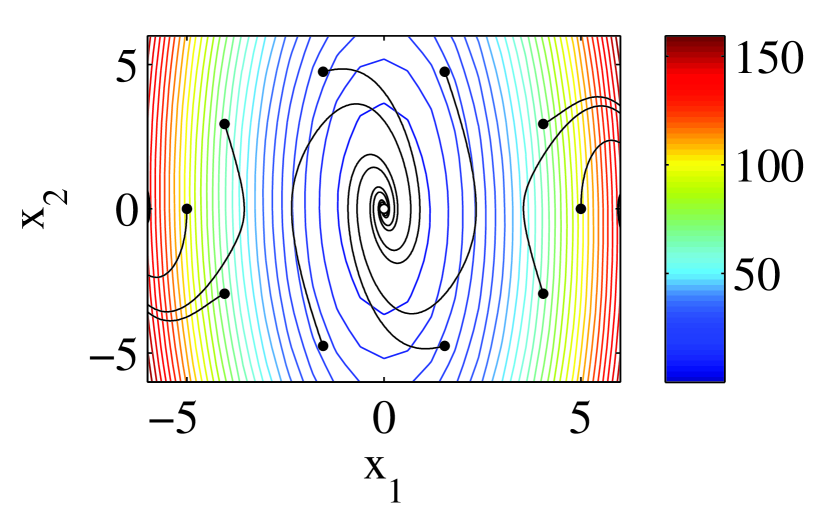
(a) The state trajectories (black lines)

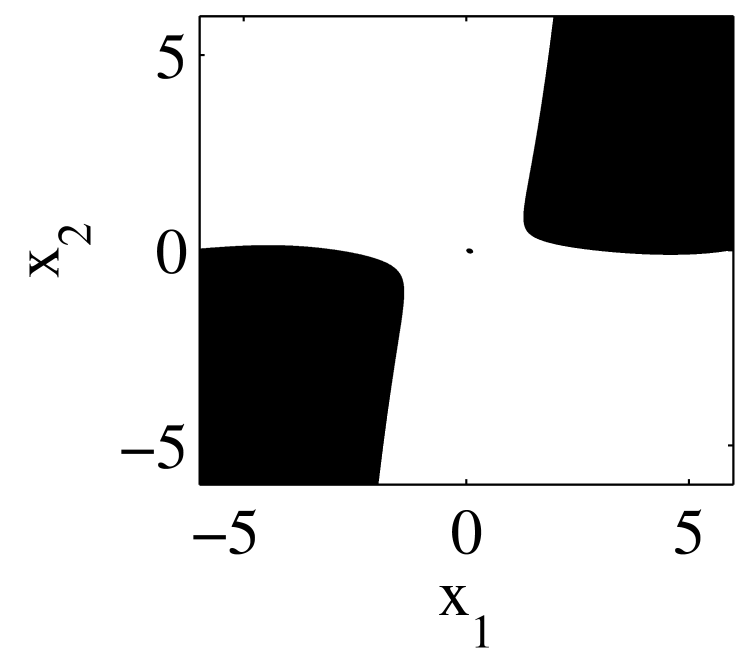
(b) The plot of $H_{\dot{V}}(\tilde{x}_{k};\alpha)$

(c) The plot of $\hat{V}(\tilde{x}_{k};\alpha)$

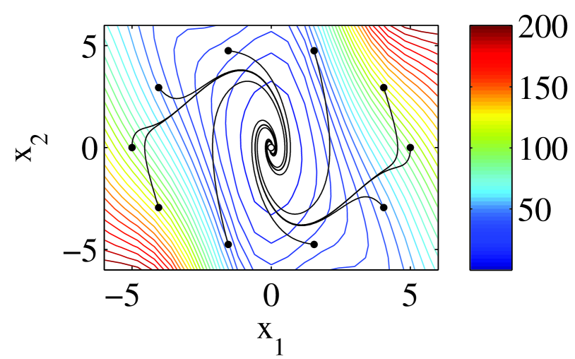
(d) The state trajectories (black lines)
 

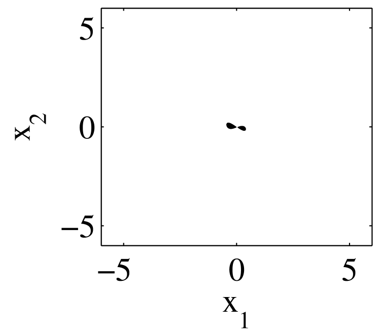
(e) The plot of $H_{\dot{V}}^{\mathrm{U}}(\tau,\mathbb{S}_{\tilde{x}};\alpha)$
$\qquad(\tau\geq 0.71\times 10^{-4})$

(f) The plot of $\hat{V}^{\mathrm{L}}(\tau,\mathbb{S}_{\tilde{x}};\alpha)$
$\qquad(\tau\geq 0.71\times 10^{-4})$

Figure 1: The pendulum example showing control and stability. The top row 1, 1, and 1 show the results of the initial controller and the bottom row 1, 1 and 1 show the proposed controller. Contours in 1 and 1 are the value function $\hat{V}(x;\alpha)$. In the remaining plots, white signifies regions of stability and black represents instability. The results in 1, 1 are optimistic since the raw values $H_{\dot{V}}(\tilde{x}_{k};\alpha)$ and $\hat{V}(\tilde{x}_{k};\alpha)$ are plotted.

6 Discussion and Future work

This paper has focused on designing a stabilizing (sub-)optimal controller of GP-based dynamics, a challenging problem in the field of data-driven control approaches. Our contributions are summarized as follows. First, we derived the second-order $O(\tau^{2})$ bounds of Gaussian kernel based functions $\Phi(x)$ with respect to the distance $\tau$ between the sampled states in Theorems 1 and 2. The derived bounds of $\Phi(x)$ are widely applicable to various functions such as polynomials, Gaussian processes (means and variances), Gaussian mixture models, and sum/product functions of them. Second, a design method of a stabilizing (sub-)optimal controller was proposed based on the HJB equation and the Lyapunov inequality. By parameterizing the value function, the derived bounds of $O(\tau^{2})$ can be applied to the stability analysis in Theorems 3.

The proposed approach can be applied to models included in the class of $\Phi(x)$. Although the variance of GP models is not covered in this paper, GP models are still advantageous because they can avoid overfitting through nonparametric Bayesian estimation. In future work, we will take account of GP variance for controlling stochastic dynamical systems.

Appendix A The proofs

A.1 The proof of Theorem 1

This subsection gives the proof of Theorem 1. First, let us consider the case of $\mathcal{N}=2$ using the definitions

$$\tilde{x}:=s_{1}\tilde{x}_{1}+s_{2}\tilde{x}_{2},$$ (38)

$$2\hat{\tau}:=\|\tilde{x}_{1}-\tilde{x}_{2}\|\leq 2\tau$$

With the additional definitions $\sigma_{aa}:=(\tilde{x}_{1}-\tilde{x}_{2})^{\mathrm{T}}\Sigma_{w}^{-1}(\tilde{x}_{1}-\tilde{x}_{2})/2$, $\sigma_{ab}:=(x^{(i)}-\tilde{x}_{2})^{\mathrm{T}}\Sigma_{w}^{-1}(\tilde{x}_{1}-\tilde{x}_{2})/2$ and $\sigma_{bb}:=(x^{(i)}-\tilde{x}_{2})^{\mathrm{T}}\Sigma_{w}^{-1}(x^{(i)}-\tilde{x}_{2})/2$, because $s_{2}=1-s_{1}$, $K^{(i)}(\tilde{x})$ can be represented as

$$K^{(i)}(\tilde{x}) =\sigma_{f}\exp\Big{(}-\frac{1}{2}\{(\tilde{x}_{1}-\tilde{x}_{2})s_{1}-(x^{(i)}-\tilde{x}_{2})\}^{\mathrm{T}}\Sigma_{w}^{-1}\{(\tilde{x}_{1}-\tilde{x}_{2})s_{1}-(x^{(i)}-\tilde{x}_{2})\}\Big{)}$$ (39)

$$=\sigma_{f}\exp(-\sigma_{aa}s_{1}^{2}+2\sigma_{ab}s_{1}-\sigma_{bb})$$

$$=\sigma_{f}\exp\Big{(}-(\sigma_{bb}-\frac{\sigma_{ab}^{2}}{\sigma_{aa}})\Big{)}\exp\Big{(}-\sigma_{aa}(s_{1}-\frac{\sigma_{ab}}{\sigma_{aa}})^{2}\Big{)}$$

$$=\acute{\sigma}_{f}\exp\Big{(}-\acute{\sigma}_{w}(2\hat{\tau}s_{1}-z^{(i)})^{2}\Big{)},$$

where $\acute{\sigma}_{w}$, $\acute{\sigma}_{f}$, and $z^{(i)}$ are the following functions of $\tilde{x}_{1}$ and $\tilde{x}_{2}$

$$\acute{\sigma}_{w} :=\sigma_{aa}/(4\hat{\tau}^{2})\leq\lambda_{\mathrm{max}}(\Sigma_{w}^{-1})/2,$$ (40)

$$\acute{\sigma}_{f} :=\sigma_{f}\exp\Big{(}-\frac{1}{\sigma_{aa}}(\sigma_{aa}\sigma_{bb}-\sigma_{ab}^{2})\Big{)},$$ (41)

$$z^{(i)} :=\frac{2\hat{\tau}\sigma_{ab}}{\sigma_{aa}}.$$ (42)

Here, $K^{(i)}(\tilde{x}_{1})=K^{(i)}(\tilde{x}(s_{1}=1))$ and $K^{(i)}(\tilde{x}_{2})=K^{(i)}(\tilde{x}(s_{1}=0))$ hold. As $\Sigma_{w}^{-1}$ is positive definite, let us define $\Sigma_{\mathrm{sqrt}}$ such that $\Sigma_{\mathrm{sqrt}}^{\mathrm{T}}\Sigma_{\mathrm{sqrt}}=\Sigma_{w}^{-1}$. With the definitions $v_{a}:=\Sigma_{\mathrm{sqrt}}(\tilde{x}_{1}-\tilde{x}_{2})$ and $v_{b}:=\Sigma_{\mathrm{sqrt}}(x^{(i)}-\tilde{x}_{2})$, because $\sigma_{aa}=\|v_{a}\|^{2}/2\geq 0$, $\sigma_{bb}=\|v_{b}\|^{2}/2$, and $\sigma_{ab}^{2}=(v_{a}^{\mathrm{T}}v_{b})^{2}/4\leq\|v_{a}\|^{2}\|v_{b}\|^{2}/4=\sigma_{aa}\sigma_{bb}$, the following inequality holds

$$\acute{\sigma}_{f}\leq\sigma_{f}.$$ (43)

Next, let us consider a $C^{2}$ function $\Psi:\mathbb{R}\rightarrow\mathbb{R}$ such that $\max_{y\in\mathbb{R}}|\Psi(y)|<\infty$, $-\infty<\min_{y\in\mathbb{R}}\partial\Psi(y)/\partial y<0$, $0<\max_{y\in\mathbb{R}}\partial\Psi(y)/\partial y<\infty$, and $\max_{y\in\mathbb{R}}|\partial^{2}\Psi(y)/\partial y^{2}|<\infty$ hold. For a given $s\in[0,1]$, $y_{1}\in\mathbb{R}$, $y_{2}:=y_{1}+2\hat{\tau}\in\mathbb{R}$ and $y(s):=sy_{1}+(1-s)y_{2}\in\mathbb{R}$, we apply the following property with respect to the linear interpolation in [7] to $\Psi(y)$

$$\Psi(y(s))-\big{\{}s\Psi(y_{1})+(1-s)\Psi(y_{2})\big{\}}=-\frac{1}{2}\frac{\partial^{2}\Psi(\hat{y})}{\partial y^{2}}(y(s)-y_{1})(y_{2}-y(s)),$$ (44)

where $\hat{y}\in[y_{1},y_{2}]$. Because of $0\leq(y(s)-y_{1})(y_{2}-y(s))\leq\hat{\tau}^{2}$, $\Psi(y)-\big{\{}s\Psi(y_{1})+(1-s)\Psi(y_{2})\big{\}}$ is bounded for any $y$, $y_{1}$ and $y_{2}$ as follows

$$\frac{\hat{\tau}^{2}}{2}\min_{y\in\mathbb{R}}\Big{(}-\frac{\partial^{2}\Psi(\hat{y})}{\partial y^{2}}\Big{)}\leq\Psi(y(s))-\big{\{}s\Psi(y_{1})+(1-s)\Psi(y_{2})\big{\}}\leq\frac{\hat{\tau}^{2}}{2}\max_{y\in\mathbb{R}}\Big{(}-\frac{\partial^{2}\Psi(\hat{y})}{\partial y^{2}}\Big{)}.$$ (45)

Substituting $\Psi(y)=\acute{\sigma}_{f}\exp(-\acute{\sigma}_{w}y^{2})$, $s=s_{1}$ and $y_{1}=z^{(i)}-2\hat{\tau}$ into (45) yields,

$$\frac{\hat{\tau}^{2}}{2}\min_{y\in\mathbb{R}}\Big{(}-\frac{\partial^{2}\Psi(\hat{y})}{\partial y^{2}}\Big{)}\leq K^{(i)}(\tilde{x})-\big{\{}s_{1}K^{(i)}(\tilde{x}_{1})+(1-s_{1})K^{(i)}(\tilde{x}_{2})\big{\}}\leq\frac{\hat{\tau}^{2}}{2}\max_{y\in\mathbb{R}}\Big{(}-\frac{\partial^{2}\Psi(\hat{y})}{\partial y^{2}}\Big{)}.$$ (46)

The derivatives of $\Psi(y)$ are as follows

$$\frac{\partial^{2}\Psi(y)}{\partial y^{2}} =2\acute{\sigma}_{f}\acute{\sigma}_{w}(2\acute{\sigma}_{w}y^{2}-1)\exp(-\acute{\sigma}_{w}y^{2}),$$ (47)

$$\frac{\partial^{3}\Psi(y)}{\partial y^{3}} =-4\acute{\sigma}_{f}\acute{\sigma}_{w}^{2}y(2\acute{\sigma}_{w}y^{2}-3)\exp(-\acute{\sigma}_{w}y^{2}).$$ (48)

From (46), (47), and (48), the lower bound $\epsilon_{K^{(i)}}^{\mathrm{L}}(\tau,\mathbb{S}_{\tilde{x}})$ of $K^{(i)}(\tilde{x})$ in the case of $\mathcal{N}=2$ is given as follows

$$-\epsilon_{K^{(i)}}^{\mathrm{L}}(\tau,\mathbb{S}_{\tilde{x}})|_{\mathcal{N}=2} =\min_{\acute{\sigma}_{f},\acute{\sigma}_{w},\hat{\tau}\leq\tau}\frac{\hat{\tau}^{2}}{2}\Big{(}-\frac{\partial^{2}\Psi(\hat{y})}{\partial y^{2}}\Big{)}\Big{|}_{y=\pm\sqrt{(3/(2\acute{\sigma}_{w}))}}=-\exp(-3/2)\sigma_{f}\lambda_{\mathrm{max}}(\Sigma_{w}^{-1})\tau^{2}.$$ (49)

The upper bound $\epsilon_{K^{(i)}}^{\mathrm{U}}(\tau,\mathbb{S}_{\tilde{x}})$ is given as

$$\epsilon_{K^{(i)}}^{\mathrm{U}}(\tau,\mathbb{S}_{\tilde{x}})|_{\mathcal{N}=2} =\max_{\acute{\sigma}_{f},\acute{\sigma}_{w},\hat{\tau}\leq\tau}\frac{\hat{\tau}^{2}}{2}\Big{(}-\frac{\partial^{2}\Psi(\hat{y})}{\partial y^{2}}\Big{)}\Big{|}_{y=0}=\sigma_{f}\lambda_{\mathrm{max}}(\Sigma_{w}^{-1})\tau^{2}/2.$$ (50)

Finally, the above results are extended to the cases $\mathcal{N}\geq 3$. The kernels are bounded by setting $\acute{s}_{k}$ and $\acute{x}_{k}$ appropriately

$$K^{(i)}(\tilde{x}) \leq\acute{s}_{1}K^{(i)}(\tilde{x}_{1})+(1-\acute{s}_{1})K^{(i)}(\acute{x}_{2})+\epsilon_{K^{(i)}}^{\mathrm{U}}(\tau,\mathbb{S}_{\tilde{x}})|_{\mathcal{N}=2}$$ (51)

$$=\acute{s}_{1}K^{(i)}(\tilde{x}_{1})+(1-\acute{s}_{1})K^{(i)}(\acute{s}_{2}\tilde{x}_{2}+(1-\acute{s}_{2})\acute{x}_{3})+\epsilon_{K^{(i)}}^{\mathrm{U}}(\tau,\mathbb{S}_{\tilde{x}})|_{\mathcal{N}=2}$$

$$\leq\acute{s}_{1}K^{(i)}(\tilde{x}_{1})+(1-\acute{s}_{1})\acute{s}_{2}K^{(i)}(\tilde{x}_{2})+(1-\acute{s}_{1})(1-\acute{s}_{2})K^{(i)}(\acute{x}_{3})$$

$$\quad+(1+(1-\acute{s}_{1}))\epsilon_{K^{(i)}}^{\mathrm{U}}(\tau,\mathbb{S}_{\tilde{x}})|_{\mathcal{N}=2}$$

$$\leq...\leq\sum_{k=1}^{\mathcal{N}}s_{k}K^{(i)}(\tilde{x}_{k})+(\mathcal{N}-1)\epsilon_{K^{(i)}}^{\mathrm{U}}(\tau,\mathbb{S}_{\tilde{x}})|_{\mathcal{N}=2},$$

where $K^{(i)}(\tilde{x})$ is bounded from below in a manner similar to the above derivation

$$K^{(i)}(\tilde{x}) \geq\sum_{k=1}^{\mathcal{N}}s_{k}K^{(i)}(\tilde{x}_{k})-(\mathcal{N}-1)\epsilon_{K^{(i)}}^{\mathrm{L}}(\tau,\mathbb{S}_{\tilde{x}})|_{\mathcal{N}=2}.$$ (52)

By substituting (49) and (50) into (51) and (52), Theorem 1 is proved. This completes the proof. $\blacksquare$

A.2 The proof of Theorem 2

Multiplying the form (9) (with respect to $\psi_{j}(\tilde{x})$) by $\phi_{j}(\tilde{x})$ gives the relations:

$$\phi_{j}(\tilde{x})\geq 0\Rightarrow-\phi_{j}(\tilde{x})\epsilon_{\psi_{j}}^{\mathrm{L}}(\tau,\mathbb{S}_{\tilde{x}})\leq\phi_{j}(\tilde{x})\{\psi_{j}(\tilde{x})-\bar{\psi}_{j}(\tilde{x})\}\leq\phi_{j}(\tilde{x})\epsilon_{\psi_{j}}^{\mathrm{U}}(\tau,\mathbb{S}_{\tilde{x}}),$$ (53)

$$\phi_{j}(\tilde{x})<0\Rightarrow-\phi_{j}(\tilde{x})\epsilon_{\psi_{j}}^{\mathrm{L}}(\tau,\mathbb{S}_{\tilde{x}})\geq\phi_{j}(\tilde{x})\{\psi_{j}(\tilde{x})-\bar{\psi}_{j}(\tilde{x})\}\geq\phi_{j}(\tilde{x})\epsilon_{\psi_{j}}^{\mathrm{U}}(\tau,\mathbb{S}_{\tilde{x}}).$$ (54)

Merging the above inequalities yields

$$-\bar{\epsilon}_{\psi_{j}}^{\mathrm{L}}(\tau,\mathbb{S}_{\tilde{x}},\phi_{j}(\tilde{x})):=-(\epsilon_{\psi_{j}}^{\mathrm{L}}(\tau,\mathbb{S}_{\tilde{x}})\max\{0,\phi_{j}(\tilde{x})\}+\epsilon_{\psi_{j}}^{\mathrm{U}}(\tau,\mathbb{S}_{\tilde{x}})\max\{0,-\phi_{j}(\tilde{x})\})$$ (55)

$$\leq\phi_{j}(\tilde{x})\{\psi_{j}(\tilde{x})-\bar{\psi}_{j}(\tilde{x})\}$$

$$\leq\bar{\epsilon}_{\psi_{j}}^{\mathrm{U}}(\tau,\mathbb{S}_{\tilde{x}},\phi_{j}(\tilde{x})):=(\epsilon_{\psi_{j}}^{\mathrm{U}}(\tau,\mathbb{S}_{\tilde{x}})\max\{0,\phi_{j}(\tilde{x})\}+\epsilon_{\psi_{j}}^{\mathrm{L}}(\tau,\mathbb{S}_{\tilde{x}})\max\{0,-\phi_{j}(\tilde{x})\}).$$

In a similar manner, multiplying the form (9) (with respect to $\phi_{j}(\tilde{x})$) by $\bar{\psi}_{j}(\tilde{x})$ yields

$$-\bar{\epsilon}_{\phi_{j}}^{\mathrm{L}}(\tau,\mathbb{S}_{\tilde{x}},\bar{\psi}_{j}(\tilde{x})):=-(\epsilon_{\phi_{j}}^{\mathrm{L}}(\tau,\mathbb{S}_{\tilde{x}})\max\{0,\bar{\psi}_{j}(\tilde{x})\}+\epsilon_{\phi_{j}}^{\mathrm{U}}(\tau,\mathbb{S}_{\tilde{x}})\max\{0,-\bar{\psi}_{j}(\tilde{x})\})$$ (56)

$$\leq\bar{\psi}_{j}(\tilde{x})\{\phi_{j}(\tilde{x})-\bar{\phi}_{j}(\tilde{x})\}$$

$$\leq\bar{\epsilon}_{\phi_{j}}^{\mathrm{U}}(\tau,\mathbb{S}_{\tilde{x}},\bar{\psi}_{j}(\tilde{x})):=(\epsilon_{\phi_{j}}^{\mathrm{U}}(\tau,\mathbb{S}_{\tilde{x}})\max\{0,\bar{\psi}_{j}(\tilde{x})\}+\epsilon_{\phi_{j}}^{\mathrm{L}}(\tau,\mathbb{S}_{\tilde{x}})\max\{0,-\bar{\psi}_{j}(\tilde{x})\}).$$

Therefore, the sum of (55) and (56) are

$$-\{\bar{\epsilon}_{\psi_{j}}^{\mathrm{L}}(\tau,\mathbb{S}_{\tilde{x}},\phi_{j}(\tilde{x}))+\bar{\epsilon}_{\phi_{j}}^{\mathrm{L}}(\tau,\mathbb{S}_{\tilde{x}},\bar{\psi}_{j}(\tilde{x}))\}$$ (57)

$$\leq\phi_{j}(\tilde{x})\psi_{j}(\tilde{x})-\bar{\phi}_{j}(\tilde{x})\bar{\psi}_{j}(\tilde{x})\leq\{\bar{\epsilon}_{\psi_{j}}^{\mathrm{U}}(\tau,\mathbb{S}_{\tilde{x}},\phi_{j}(\tilde{x}))+\bar{\epsilon}_{\phi_{j}}^{\mathrm{U}}(\tau,\mathbb{S}_{\tilde{x}},\bar{\psi}_{j}(\tilde{x}))\}.$$

Here, $\bar{\phi}_{j}(\tilde{x})\bar{\psi}_{j}(\tilde{x})$ is transformed as follows

$$\bar{\phi}_{j}(\tilde{x})\bar{\psi}_{j}(\tilde{x})$$ (58)

$$=\sum_{k=1}^{\mathcal{N}}s_{k}\phi_{j}(\tilde{x}_{k})\psi_{j}(\tilde{x}_{k})+\sum_{k=1}^{\mathcal{N}}s_{k}(s_{k}-1)\phi_{j}(\tilde{x}_{k})\psi_{j}(\tilde{x}_{k})+\sum_{k=1}^{\mathcal{N}}\sum_{l=1,l\neq k}^{\mathcal{N}}s_{k}s_{l}\phi_{j}(\tilde{x}_{k})\psi_{j}(\tilde{x}_{l})$$

$$=\sum_{k=1}^{\mathcal{N}}s_{k}\phi_{j}(\tilde{x}_{k})\psi_{j}(\tilde{x}_{k})-\sum_{k=1}^{\mathcal{N}}s_{k}(\sum_{l=1,l\neq k}^{\mathcal{N}}s_{l})\phi_{j}(\tilde{x}_{k})\psi_{j}(\tilde{x}_{k})+\sum_{k=1}^{\mathcal{N}}\sum_{l=1,l\neq k}^{\mathcal{N}}s_{k}s_{l}\phi_{j}(\tilde{x}_{k})\psi_{j}(\tilde{x}_{l})$$

$$=\sum_{k=1}^{\mathcal{N}}s_{k}\phi_{j}(\tilde{x}_{k})\psi_{j}(\tilde{x}_{k})+\sum_{k=1}^{\mathcal{N}}\sum_{l=1,l\neq k}^{\mathcal{N}}s_{k}s_{l}\phi_{j}(\tilde{x}_{k})(\psi_{j}(\tilde{x}_{l})-\psi_{j}(\tilde{x}_{k}))$$

$$=\sum_{k=1}^{\mathcal{N}}s_{k}\phi_{j}(\tilde{x}_{k})\psi_{j}(\tilde{x}_{k})+\sum_{k=1}^{\mathcal{N}}\sum_{l=1,l>k}^{\mathcal{N}}s_{k}s_{l}\phi_{j}(\tilde{x}_{k})(\psi_{j}(\tilde{x}_{l})-\psi_{j}(\tilde{x}_{k}))$$

$$\quad+\sum_{k=1}^{\mathcal{N}}\sum_{l=1,l<k}^{\mathcal{N}}s_{k}s_{l}\phi_{j}(\tilde{x}_{k})(\psi_{j}(\tilde{x}_{l})-\psi_{j}(\tilde{x}_{k}))$$

$$=\sum_{k=1}^{\mathcal{N}}s_{k}\phi_{j}(\tilde{x}_{k})\psi_{j}(\tilde{x}_{k})+\sum_{k=1}^{\mathcal{N}}\sum_{l=1,l>k}^{\mathcal{N}}s_{k}s_{l}\phi_{j}(\tilde{x}_{k})(\psi_{j}(\tilde{x}_{l})-\psi_{j}(\tilde{x}_{k}))$$

$$\quad+\sum_{k=1}^{\mathcal{N}}\sum_{l=1,l>k}^{\mathcal{N}}s_{k}s_{l}\phi_{j}(\tilde{x}_{l})(\psi_{j}(\tilde{x}_{k})-\psi_{j}(\tilde{x}_{l}))$$

$$=\sum_{k=1}^{\mathcal{N}}s_{k}\phi_{j}(\tilde{x}_{k})\psi_{j}(\tilde{x}_{k})+\sum_{k=1}^{\mathcal{N}-1}\sum_{l=k+1}^{\mathcal{N}}s_{k}s_{l}\{\phi_{j}(\tilde{x}_{k})-\phi_{j}(\tilde{x}_{l})\}\{\psi_{j}(\tilde{x}_{l})-\psi_{j}(\tilde{x}_{k})\}$$

$$=:\sum_{k=1}^{\mathcal{N}}s_{k}\phi_{j}(\tilde{x}_{k})\psi_{j}(\tilde{x}_{k})+4\tau^{2}\sum_{k=1}^{\mathcal{N}-1}\sum_{l=k+1}^{\mathcal{N}}s_{k}s_{l}\mathcal{L}_{\phi_{j},\psi_{j}}(\tau,\tilde{x}_{k},\tilde{x}_{l}),$$

where because $\|\tilde{x}_{k}-\tilde{x}_{l}\|\leq 2\tau$ and $\phi_{j}(x)$ and $\psi_{j}(x)$ are Lipschitz continuous,

$$\mathcal{L}_{\phi_{j},\psi_{j}}(\tau,\tilde{x}_{k},\tilde{x}_{l}) :=\frac{\phi_{j}(\tilde{x}_{k})-\phi_{j}(\tilde{x}_{l})}{2\tau}\frac{\psi_{j}(\tilde{x}_{l})-\psi_{j}(\tilde{x}_{k})}{2\tau}=O(1),\quad\mathrm{as}\quad\tau\rightarrow 0.$$ (59)

As $\sum_{k=1}^{\mathcal{N}-1}\sum_{l=k+1}^{\mathcal{N}}s_{k}s_{l}\leq\sum_{k=1}^{\mathcal{N}}\sum_{l=1}^{\mathcal{N}}s_{k}s_{l}\leq 1$ and $s_{k}s_{l}\geq 0$ for all $k$ and $l$, we obtain

$$\min_{k,l}\mathcal{L}_{\phi_{j},\psi_{j}}(\tau,\tilde{x}_{k},\tilde{x}_{l}) =\min\{0,\min_{k,l\;(k\neq l)}\mathcal{L}_{\phi_{j},\psi_{j}}(\tau,\tilde{x}_{k},\tilde{x}_{l})\}$$

$$\leq\sum_{k=1}^{\mathcal{N}-1}\sum_{l=k+1}^{\mathcal{N}}s_{k}s_{l}\mathcal{L}_{\phi_{j},\psi_{j}}(\tau,\tilde{x}_{k},\tilde{x}_{l})$$

$$\leq\max\{0,\max_{k,l\;(k\neq l)}\mathcal{L}_{\phi_{j},\psi_{j}}(\tau,\tilde{x}_{k},\tilde{x}_{l})\}$$

$$=\max_{k,l}\mathcal{L}_{\phi_{j},\psi_{j}}(\tau,\tilde{x}_{k},\tilde{x}_{l}),$$ (60)

$$\min_{k,l}\sum_{j=1}^{\mathcal{M}}\mathcal{L}_{\phi_{j},\psi_{j}}(\tau,\tilde{x}_{k},\tilde{x}_{l}) \leq\sum_{j=1}^{\mathcal{M}}\sum_{k=1}^{\mathcal{N}-1}\sum_{l=k+1}^{\mathcal{N}}s_{k}s_{l}\mathcal{L}_{\phi_{j},\psi_{j}}(\tau,\tilde{x}_{k},\tilde{x}_{l})$$

$$=\sum_{k=1}^{\mathcal{N}-1}\sum_{l=k+1}^{\mathcal{N}}\sum_{j=1}^{\mathcal{M}}s_{k}s_{l}\mathcal{L}_{\phi_{j},\psi_{j}}(\tau,\tilde{x}_{k},\tilde{x}_{l})$$

$$\leq\max_{k,l}\sum_{j=1}^{\mathcal{M}}\mathcal{L}_{\phi_{j},\psi_{j}}(\tau,\tilde{x}_{k},\tilde{x}_{l})$$ (61)

Substituting (58) into (57) yields

$$-\{\bar{\epsilon}_{\psi_{j}}^{\mathrm{L}}(\tau,\mathbb{S}_{\tilde{x}},\phi_{j}(\tilde{x}))+\bar{\epsilon}_{\phi_{j}}^{\mathrm{L}}(\tau,\mathbb{S}_{\tilde{x}},\bar{\psi}_{j}(\tilde{x}))\}+4\tau^{2}\min_{k,l}\mathcal{L}_{\phi_{j},\psi_{j}}(\tau,\tilde{x}_{k},\tilde{x}_{l})$$ (62)

$$\leq\phi_{j}(\tilde{x})\psi_{j}(\tilde{x})-\sum_{k=1}^{\mathcal{N}}s_{k}\phi_{j}(\tilde{x}_{k})\psi_{j}(\tilde{x}_{k})$$

$$\leq\{\bar{\epsilon}_{\psi_{j}}^{\mathrm{U}}(\tau,\mathbb{S}_{\tilde{x}},\phi_{j}(\tilde{x}))+\bar{\epsilon}_{\phi_{j}}^{\mathrm{U}}(\tau,\mathbb{S}_{\tilde{x}},\bar{\psi}_{j}(\tilde{x}))\}+4\tau^{2}\max_{k,l}\mathcal{L}_{\phi_{j},\psi_{j}}(\tau,\tilde{x}_{k},\tilde{x}_{l}).$$

Consequently, the sum of (62) for all $j$ is

$$-\max_{\tilde{x}\in\mathbb{S}_{\tilde{x}}}\sum_{j=1}^{\mathcal{M}}\{\bar{\epsilon}_{\psi_{j}}^{\mathrm{L}}(\tau,\mathbb{S}_{\tilde{x}},\phi_{j}(\tilde{x}))+\bar{\epsilon}_{\phi_{j}}^{\mathrm{L}}(\tau,\mathbb{S}_{\tilde{x}},\bar{\psi}_{j}(\tilde{x}))\}+4\tau^{2}\min_{k,l}\sum_{j=1}^{\mathcal{M}}\mathcal{L}_{\phi_{j},\psi_{j}}(\tau,\tilde{x}_{k},\tilde{x}_{l})$$ (63)

$$\leq\sum_{j=1}^{\mathcal{M}}\phi_{j}(\tilde{x})\psi_{j}(\tilde{x})-\sum_{k=1}^{\mathcal{N}}s_{k}\sum_{j=1}^{\mathcal{M}}\phi_{j}(\tilde{x}_{k})\psi_{j}(\tilde{x}_{k})$$

$$=\chi(\tilde{x})-\bar{\chi}(\tilde{x})$$

$$\leq\max_{\tilde{x}\in\mathbb{S}_{\tilde{x}}}\sum_{j=1}^{\mathcal{M}}\{\bar{\epsilon}_{\psi_{j}}^{\mathrm{U}}(\tau,\mathbb{S}_{\tilde{x}},\phi_{j}(\tilde{x}))+\bar{\epsilon}_{\phi_{j}}^{\mathrm{U}}(\tau,\mathbb{S}_{\tilde{x}},\bar{\psi}_{j}(\tilde{x}))\}+4\tau^{2}\max_{k,l}\sum_{j=1}^{\mathcal{M}}\mathcal{L}_{\phi_{j},\psi_{j}}(\tau,\tilde{x}_{k},\tilde{x}_{l}).$$

Here, the following property holds. First, $\bar{\psi}_{j}(\tilde{x})$ is a function of $s_{k}$ and $\bar{\psi}_{j}(s_{1},...,s_{\mathcal{N}})$ is linear in $s_{\mathrm{vec}}:=[s_{1},...,s_{\mathcal{N}}]$. Because of such a linearity, $\sum_{j=1}^{\mathcal{M}}\epsilon_{\phi_{j}}^{\mathrm{L}}(\tau,\mathbb{S}_{\tilde{x}})\max\{0,\bar{\psi}_{j}(s_{1},...,s_{\mathcal{N}})\}$ is convex in $s_{\mathrm{vec}}$. As $s_{\mathrm{vec}}$ are defined on the set such that $s_{k}\geq 0$ and $\sum_{k=1}^{\mathcal{N}}s_{k}=1$, this convex function has a maximum value at the vertices $s_{\mathrm{vec}}^{(k)}$ for some $k$, where $s_{\mathrm{vec}}^{(k)}$ is defined such that the $k$-th component is $1$ and the other components are $0$. This property gives

$$\mathcal{S}_{\phi,\bar{\psi}}^{\mathrm{L}}(\tau,\mathbb{S}_{\tilde{x}}) :=\max_{\tilde{x}}\sum_{j=1}^{\mathcal{M}}\bar{\epsilon}_{\phi_{j}}^{\mathrm{L}}(\tau,\mathbb{S}_{\tilde{x}},\bar{\psi}_{j}(\tilde{x}))$$ (64)

$$=\max_{\tilde{x}}\sum_{j=1}^{\mathcal{M}}(\epsilon_{\phi_{j}}^{\mathrm{L}}(\tau,\mathbb{S}_{\tilde{x}})\max\{0,\bar{\psi}_{j}(\tilde{x})\}+\epsilon_{\phi_{j}}^{\mathrm{U}}(\tau,\mathbb{S}_{\tilde{x}})\max\{0,-\bar{\psi}_{j}(\tilde{x})\})$$

$$=\max_{k}\sum_{j=1}^{\mathcal{M}}(\epsilon_{\phi_{j}}^{\mathrm{L}}(\tau,\mathbb{S}_{\tilde{x}})\max\{0,\psi_{j}(\tilde{x}_{k})\}+\epsilon_{\phi_{j}}^{\mathrm{U}}(\tau,\mathbb{S}_{\tilde{x}})\max\{0,-\psi_{j}(\tilde{x}_{k})\}),$$

$$\mathcal{S}_{\phi,\bar{\psi}}^{\mathrm{U}}(\tau,\mathbb{S}_{\tilde{x}}) :=\max_{\tilde{x}}\sum_{j=1}^{\mathcal{M}}\bar{\epsilon}_{\phi_{j}}^{\mathrm{U}}(\tau,\mathbb{S}_{\tilde{x}},\bar{\psi}_{j}(\tilde{x}))$$ (65)

$$=\max_{k}\sum_{j=1}^{\mathcal{M}}(\epsilon_{\phi_{j}}^{\mathrm{U}}(\tau,\mathbb{S}_{\tilde{x}})\max\{0,\psi_{j}(\tilde{x}_{k})\}+\epsilon_{\phi_{j}}^{\mathrm{L}}(\tau,\mathbb{S}_{\tilde{x}})\max\{0,-\psi_{j}(\tilde{x}_{k})\}).$$

In a similar manner, the following inequalities are obtained using the bounds of $\phi_{j}(\tilde{x})$

$$\max_{\tilde{x}}\sum_{j=1}^{\mathcal{M}}\bar{\epsilon}_{\psi_{j}}^{\mathrm{L}}(\tau,\mathbb{S}_{\tilde{x}},\phi_{j}(\tilde{x}))$$ (66)

$$=\max_{\tilde{x}}\sum_{j=1}^{\mathcal{M}}(\epsilon_{\psi_{j}}^{\mathrm{L}}(\tau,\mathbb{S}_{\tilde{x}})\max\{0,\phi_{j}(\tilde{x})\}+\epsilon_{\psi_{j}}^{\mathrm{U}}(\tau,\mathbb{S}_{\tilde{x}})\max\{0,-\phi_{j}(\tilde{x})\})$$

$$\leq\max_{\tilde{x}}\sum_{j=1}^{\mathcal{M}}\Big{(}\epsilon_{\psi_{j}}^{\mathrm{L}}(\tau,\mathbb{S}_{\tilde{x}})\max\{0,\bar{\phi}_{j}(\tilde{x})+\epsilon_{\phi_{j}}^{\mathrm{U}}(\tau,\mathbb{S}_{\tilde{x}})\}$$

$$\qquad\qquad+\epsilon_{\psi_{j}}^{\mathrm{U}}(\tau,\mathbb{S}_{\tilde{x}})\max\{0,-\bar{\phi}_{j}(\tilde{x})+\epsilon_{\phi_{j}}^{\mathrm{L}}(\tau,\mathbb{S}_{\tilde{x}})\}\Big{)}$$

$$\leq\max_{\tilde{x}}\sum_{j=1}^{\mathcal{M}}\Big{(}\epsilon_{\psi_{j}}^{\mathrm{L}}(\tau,\mathbb{S}_{\tilde{x}})\max\{0,\bar{\phi}_{j}(\tilde{x})\}+\epsilon_{\psi_{j}}^{\mathrm{L}}(\tau,\mathbb{S}_{\tilde{x}})\epsilon_{\phi_{j}}^{\mathrm{U}}(\tau,\mathbb{S}_{\tilde{x}})$$

$$\qquad\qquad+\epsilon_{\psi_{j}}^{\mathrm{U}}(\tau,\mathbb{S}_{\tilde{x}})\max\{0,-\bar{\phi}_{j}(\tilde{x})\}+\epsilon_{\psi_{j}}^{\mathrm{U}}(\tau,\mathbb{S}_{\tilde{x}})\epsilon_{\phi_{j}}^{\mathrm{L}}(\tau,\mathbb{S}_{\tilde{x}})\Big{)}$$

$$=\mathcal{S}_{\psi,\bar{\phi}}^{\mathrm{L}}(\tau,\mathbb{S}_{\tilde{x}})+\sum_{j=1}^{\mathcal{M}}\Big{(}\epsilon_{\psi_{j}}^{\mathrm{L}}(\tau,\mathbb{S}_{\tilde{x}})\epsilon_{\phi_{j}}^{\mathrm{U}}(\tau,\mathbb{S}_{\tilde{x}})+\epsilon_{\psi_{j}}^{\mathrm{U}}(\tau,\mathbb{S}_{\tilde{x}})\epsilon_{\phi_{j}}^{\mathrm{L}}(\tau,\mathbb{S}_{\tilde{x}})\Big{)}.$$

$$\max_{\tilde{x}}\sum_{j=1}^{\mathcal{M}}\bar{\epsilon}_{\psi_{j}}^{\mathrm{U}}(\tau,\mathbb{S}_{\tilde{x}},\phi_{j}(\tilde{x}))$$ (67)

$$\leq\mathcal{S}_{\psi,\bar{\phi}}^{\mathrm{U}}(\tau,\mathbb{S}_{\tilde{x}})+\sum_{j=1}^{\mathcal{M}}\Big{(}\epsilon_{\psi_{j}}^{\mathrm{U}}(\tau,\mathbb{S}_{\tilde{x}})\epsilon_{\phi_{j}}^{\mathrm{U}}(\tau,\mathbb{S}_{\tilde{x}})+\epsilon_{\psi_{j}}^{\mathrm{L}}(\tau,\mathbb{S}_{\tilde{x}})\epsilon_{\phi_{j}}^{\mathrm{L}}(\tau,\mathbb{S}_{\tilde{x}})\Big{)}.$$

Substituting (64), (65), (66), and (67) into (63) yields

$$-\mathcal{S}_{\phi,\bar{\psi}}^{\mathrm{L}}(\tau,\mathbb{S}_{\tilde{x}})-\mathcal{S}_{\psi,\bar{\phi}}^{\mathrm{L}}(\tau,\mathbb{S}_{\tilde{x}})-\sum_{j=1}^{\mathcal{M}}\Big{(}\epsilon_{\psi_{j}}^{\mathrm{L}}(\tau,\mathbb{S}_{\tilde{x}})\epsilon_{\phi_{j}}^{\mathrm{U}}(\tau,\mathbb{S}_{\tilde{x}})+\epsilon_{\psi_{j}}^{\mathrm{U}}(\tau,\mathbb{S}_{\tilde{x}})\epsilon_{\phi_{j}}^{\mathrm{L}}(\tau,\mathbb{S}_{\tilde{x}})\Big{)}$$ (68)

$$\qquad+4\tau^{2}\min_{k,l}\sum_{j=1}^{\mathcal{M}}\mathcal{L}_{\phi_{j},\psi_{j}}(\tau,\tilde{x}_{k},\tilde{x}_{l})$$

$$\leq\chi(\tilde{x})-\bar{\chi}(\tilde{x})$$

$$\leq\mathcal{S}_{\phi,\bar{\psi}}^{\mathrm{U}}(\tau,\mathbb{S}_{\tilde{x}})+\mathcal{S}_{\psi,\bar{\phi}}^{\mathrm{U}}(\tau,\mathbb{S}_{\tilde{x}})+\sum_{j=1}^{\mathcal{M}}\Big{(}\epsilon_{\psi_{j}}^{\mathrm{U}}(\tau,\mathbb{S}_{\tilde{x}})\epsilon_{\phi_{j}}^{\mathrm{U}}(\tau,\mathbb{S}_{\tilde{x}})+\epsilon_{\psi_{j}}^{\mathrm{L}}(\tau,\mathbb{S}_{\tilde{x}})\epsilon_{\phi_{j}}^{\mathrm{L}}(\tau,\mathbb{S}_{\tilde{x}})\Big{)}$$

$$\qquad+4\tau^{2}\max_{k,l}\sum_{j=1}^{\mathcal{M}}\mathcal{L}_{\phi_{j},\psi_{j}}(\tau,\tilde{x}_{k},\tilde{x}_{l}).$$

Consequently, the lower and upper bounds $\epsilon_{\chi}^{\mathrm{L}}(\tau,\mathbb{S}_{\tilde{x}})$ and $\epsilon_{\chi}^{\mathrm{U}}(\tau,\mathbb{S}_{\tilde{x}})$ of the function $\chi(\tilde{x})$ are $O(\tau^{2})$ as follows

$$\epsilon_{\chi}^{\mathrm{L}}(\tau,\mathbb{S}_{\tilde{x}}) =\mathcal{S}_{\phi,\bar{\psi}}^{\mathrm{L}}(\tau,\mathbb{S}_{\tilde{x}})+\mathcal{S}_{\psi,\bar{\phi}}^{\mathrm{L}}(\tau,\mathbb{S}_{\tilde{x}})+\sum_{j=1}^{\mathcal{M}}\Big{(}\epsilon_{\psi_{j}}^{\mathrm{L}}(\tau,\mathbb{S}_{\tilde{x}})\epsilon_{\phi_{j}}^{\mathrm{U}}(\tau,\mathbb{S}_{\tilde{x}})+\epsilon_{\psi_{j}}^{\mathrm{U}}(\tau,\mathbb{S}_{\tilde{x}})\epsilon_{\phi_{j}}^{\mathrm{L}}(\tau,\mathbb{S}_{\tilde{x}})\Big{)}$$

$$\quad-4\tau^{2}\min_{k,l}\sum_{j=1}^{\mathcal{M}}\mathcal{L}_{\phi_{j},\psi_{j}}(\tau,\tilde{x}_{k},\tilde{x}_{l}),$$ (69)

$$\epsilon_{\chi}^{\mathrm{U}}(\tau,\mathbb{S}_{\tilde{x}}) =\mathcal{S}_{\phi,\bar{\psi}}^{\mathrm{U}}(\tau,\mathbb{S}_{\tilde{x}})+\mathcal{S}_{\psi,\bar{\phi}}^{\mathrm{U}}(\tau,\mathbb{S}_{\tilde{x}})+\sum_{j=1}^{\mathcal{M}}\Big{(}\epsilon_{\psi_{j}}^{\mathrm{U}}(\tau,\mathbb{S}_{\tilde{x}})\epsilon_{\phi_{j}}^{\mathrm{U}}(\tau,\mathbb{S}_{\tilde{x}})+\epsilon_{\psi_{j}}^{\mathrm{L}}(\tau,\mathbb{S}_{\tilde{x}})\epsilon_{\phi_{j}}^{\mathrm{L}}(\tau,\mathbb{S}_{\tilde{x}})\Big{)}$$

$$\quad+4\tau^{2}\max_{k,l}\sum_{j=1}^{\mathcal{M}}\mathcal{L}_{\phi_{j},\psi_{j}}(\tau,\tilde{x}_{k},\tilde{x}_{l}).$$ (70)

This completes the proof. $\blacksquare$

A.3 The proof of Theorem 3

To begin, the partial derivative of the Gaussian kernel $K^{(i)}(x)$ in (5) is included in the class of $\Phi(x)$ as follows

$$\frac{\partial K^{(i)}(x)}{\partial x} =-\Sigma_{w}^{-1}(x-x^{(i)})K^{(i)}(x).$$ (71)

Also, all components of the partial derivative of $\phi_{j,k}(x)$ are included in the class of $\Phi(x)$. Thus, the partial derivative of $\Phi(x)$ is included in the class of $\Phi(x)$. Also, products and sums of $\Phi(x)$ are included in the class of $\Phi(x)$.

From the assumptions in Theorem 3, all components of $\hat{f}(x)$, $\hat{g}(x)$, $R(x)^{-1}$, and $\hat{V}(x)$ are included in the class of $\Phi(x)$. All components of $\hat{p}(x;\alpha)$, which is the partial derivative of $\hat{V}(x;\alpha)$, are included in the class of $\Phi(x)$. The function $H_{\dot{V}}(x,\hat{V}(x;\alpha))$ is included in the class of $\Phi(x)$ because $H_{\dot{V}}(x,\hat{V}(x;\alpha))$ consists of sums and products of the functions in the class of $\Phi(x)$. Therefore, by iterating Theorem 2, the $O(\tau^{2})$ bounds of $\hat{V}(x)$ and $H_{\dot{V}}(x,\hat{V}(x;\alpha))$ are explicitly obtained. This completes the proof. $\blacksquare$

In the following, we derive the bound in the case that $\hat{f}(x)$ obeys (28), $\hat{g}$ and $R$ are constant, and $\hat{V}(x;\alpha)$ is defined as $\hat{V}(x;\alpha):=\{\sum_{i=1}^{D}[\alpha]_{i}K^{(i)}(x)\}-\{\sum_{i=1}^{D}[\alpha]_{i}K^{(i)}(x)|_{x=0}\}$. The closed loop ${f_{\mathrm{cl}}}(x;\alpha)$ with the (sub-)optimal input in (31) and $\hat{p}(x;\alpha)$ are given by

$$[\hat{p}(x;\alpha)]_{j} \;=\sum_{i=1}^{D}[\mathcal{P}^{(i)}(x;\alpha)]_{j}K^{(i)}(x),$$ (72)

$$\mathcal{P}^{(i)}(x;\alpha) :=-[\alpha]_{i}\Sigma_{w}^{-1}(x-x^{(i)}),$$ (73)

$$[{f_{\mathrm{cl}}}(x;\alpha)]_{j} :=\hat{f}(x)-gR^{-1}g^{\mathrm{T}}\hat{p}(x;\alpha)=\sum_{i=1}^{D}[\mathcal{A}^{(i)}(x;\alpha)]_{j}K^{(i)}(x),$$ (74)

$$\mathcal{A}^{(i)}(x;\alpha) :=[[f_{\mathrm{d}}^{(1)},f_{\mathrm{d}}^{(2)},...,f_{\mathrm{d}}^{(D)}]^{\mathrm{T}}K_{XX}^{-1}]_{\cdot,i}-gR^{-1}g^{\mathrm{T}}\mathcal{P}^{(i)}(x;\alpha).$$ (75)

Based on Theorem 2, the bounds of ${f_{\mathrm{cl}}}(\tilde{x})$ and $\hat{p}(\tilde{x};\alpha)$ are

$$\epsilon_{[\hat{p}]_{j}}^{\mathrm{L}}(\tau,\mathbb{S}_{\tilde{x}};\alpha) :=\mathcal{S}_{K,[\bar{\mathcal{P}}]_{j}}^{\mathrm{L}}(\tau,\mathbb{S}_{\tilde{x}};\alpha)-4\tau^{2}\min_{k,l}\sum_{i=1}^{D}\mathcal{L}_{[\mathcal{P}^{(i)}]_{j},K^{(i)}}(\tau,\tilde{x}_{k},\tilde{x}_{l};\alpha),$$ (76)

$$\epsilon_{[\hat{p}]_{j}}^{\mathrm{U}}(\tau,\mathbb{S}_{\tilde{x}};\alpha) :=\mathcal{S}_{K,[\bar{\mathcal{P}}]_{j}}^{\mathrm{U}}(\tau,\mathbb{S}_{\tilde{x}};\alpha)+4\tau^{2}\max_{k,l}\sum_{i=1}^{D}\mathcal{L}_{[\mathcal{P}^{(i)}]_{j},K^{(i)}}(\tau,\tilde{x}_{k},\tilde{x}_{l};\alpha),$$ (77)

$$\mathcal{S}_{K,[\bar{\mathcal{P}}]_{j}}^{\mathrm{L}}(\tau,\mathbb{S}_{\tilde{x}};\alpha)$$

$$=\max_{k}\sum_{i=1}^{D}(\epsilon_{K^{(i)}}^{\mathrm{L}}(\tau,\mathbb{S}_{\tilde{x}};\alpha)\max\{0,[{\mathcal{P}}^{(i)}(\tilde{x}_{k};\alpha)]_{j}\}+\epsilon_{K^{(i)}}^{\mathrm{U}}(\tau,\mathbb{S}_{\tilde{x}};\alpha)\max\{0,-[{\mathcal{P}}^{(i)}(\tilde{x}_{k};\alpha)]_{j}\}),$$ (78)

$$\mathcal{S}_{K,[\bar{\mathcal{P}}]_{j}}^{\mathrm{U}}(\tau,\mathbb{S}_{\tilde{x}};\alpha)$$

$$=\max_{k}\sum_{i=1}^{D}(\epsilon_{K^{(i)}}^{\mathrm{U}}(\tau,\mathbb{S}_{\tilde{x}};\alpha)\max\{0,[{\mathcal{P}}^{(i)}(\tilde{x}_{k};\alpha)]_{j}\}+\epsilon_{K^{(i)}}^{\mathrm{L}}(\tau,\mathbb{S}_{\tilde{x}};\alpha)\max\{0,-[{\mathcal{P}}^{(i)}(\tilde{x}_{k};\alpha)]_{j}\}),$$ (79)

$$\epsilon_{[{f_{\mathrm{cl}}}]_{j}}^{\mathrm{L}}(\tau,\mathbb{S}_{\tilde{x}};\alpha) :=\mathcal{S}_{K,[\bar{\mathcal{A}}]_{j}}^{\mathrm{L}}(\tau,\mathbb{S}_{\tilde{x}};\alpha)-4\tau^{2}\min_{k,l}\sum_{i=1}^{D}\mathcal{L}_{[\mathcal{A}^{(i)}]_{j},K^{(i)}}(\tau,\tilde{x}_{k},\tilde{x}_{l};\alpha),$$ (80)

$$\epsilon_{[{f_{\mathrm{cl}}}]_{j}}^{\mathrm{U}}(\tau,\mathbb{S}_{\tilde{x}};\alpha) :=\mathcal{S}_{K,[\bar{\mathcal{A}}]_{j}}^{\mathrm{U}}(\tau,\mathbb{S}_{\tilde{x}};\alpha)+4\tau^{2}\max_{k,l}\sum_{i=1}^{D}\mathcal{L}_{[\mathcal{A}^{(i)}]_{j},K^{(i)}}(\tau,\tilde{x}_{k},\tilde{x}_{l};\alpha),$$ (81)

$$\mathcal{S}_{K,[\bar{\mathcal{A}}]_{j}}^{\mathrm{L}}(\tau,\mathbb{S}_{\tilde{x}};\alpha)$$

$$=\max_{k}\sum_{i=1}^{D}(\epsilon_{K^{(i)}}^{\mathrm{L}}(\tau,\mathbb{S}_{\tilde{x}};\alpha)\max\{0,[{\mathcal{A}}^{(i)}(\tilde{x}_{k};\alpha)]_{j}\}+\epsilon_{K^{(i)}}^{\mathrm{U}}(\tau,\mathbb{S}_{\tilde{x}};\alpha)\max\{0,-[{\mathcal{A}}^{(i)}(\tilde{x}_{k};\alpha)]_{j}\}),$$ (82)

$$\mathcal{S}_{K,[\bar{\mathcal{A}}]_{j}}^{\mathrm{U}}(\tau,\mathbb{S}_{\tilde{x}};\alpha)$$

$$=\max_{k}\sum_{i=1}^{D}(\epsilon_{K^{(i)}}^{\mathrm{U}}(\tau,\mathbb{S}_{\tilde{x}};\alpha)\max\{0,[{\mathcal{A}}^{(i)}(\tilde{x}_{k};\alpha)]_{j}\}+\epsilon_{K^{(i)}}^{\mathrm{L}}(\tau,\mathbb{S}_{\tilde{x}};\alpha)\max\{0,-[{\mathcal{A}}^{(i)}(\tilde{x}_{k};\alpha)]_{j}\}).$$ (83)

The Lyapunov inequality is given by

$$H_{\dot{V}}(\tilde{x},\hat{V}(\tilde{x};\alpha))=\sum_{j=1}^{n}[\hat{p}(\tilde{x};\alpha)]_{j}[{f_{\mathrm{cl}}}(\tilde{x};\alpha)]_{j}.$$ (84)

Therefore, the bounds of $\hat{V}(\tilde{x};\alpha)$ and $H_{\dot{V}}(\tilde{x},\hat{V}(\tilde{x};\alpha))$ are

$$\epsilon_{\hat{V}}^{\mathrm{L}}(\tau,\mathbb{S}_{\tilde{x}};\alpha) =\sum_{i=1}^{D}\Big{(}\epsilon_{K^{(i)}}^{\mathrm{L}}(\tau,\mathbb{S}_{\tilde{x}};\alpha)\max\{0,[\alpha]_{i}\}+\epsilon_{K^{(i)}}^{\mathrm{U}}(\tau,\mathbb{S}_{\tilde{x}};\alpha)\max\{0,-[\alpha]_{i}\}\Big{)}=O(\tau^{2}),$$ (85)

$$\epsilon_{H_{\dot{V}}}^{\mathrm{U}}(\tau,\mathbb{S}_{\tilde{x}};\alpha)$$

$$=\max_{k}\sum_{j=1}^{n}\Big{(}\epsilon_{[\hat{p}]_{j}}^{\mathrm{U}}(\tau,\mathbb{S}_{\tilde{x}};\alpha)\max\{0,[{{f_{\mathrm{cl}}}}(\tilde{x}_{k};\alpha)]_{j}\}+\epsilon_{[\hat{p}]_{j}}^{\mathrm{L}}(\tau,\mathbb{S}_{\tilde{x}};\alpha)\max\{0,-[{{f_{\mathrm{cl}}}}(\tilde{x}_{k};\alpha)]_{j}\}\Big{)}$$

$$\quad+\max_{k}\sum_{j=1}^{n}\Big{(}\epsilon_{[{f_{\mathrm{cl}}}]_{j}}^{\mathrm{U}}(\tau,\mathbb{S}_{\tilde{x}};\alpha)\max\{0,[{\hat{p}}(\tilde{x}_{k};\alpha)]_{j}\}+\epsilon_{[{f_{\mathrm{cl}}}]_{j}}^{\mathrm{L}}(\tau,\mathbb{S}_{\tilde{x}};\alpha)\max\{0,-[{\hat{p}}(\tilde{x}_{k};\alpha)]_{j}\}\Big{)}$$

$$\quad+4\tau^{2}\max_{k,l}\sum_{j=1}^{n}\mathcal{L}_{[\hat{p}]_{j},[{f_{\mathrm{cl}}}]_{j}}(\tau,\tilde{x}_{k},\tilde{x}_{l};\alpha)$$

$$\quad+\sum_{j=1}^{n}\Big{(}\epsilon_{[{f_{\mathrm{cl}}}]_{j}}^{\mathrm{U}}(\tau,\mathbb{S}_{\tilde{x}};\alpha)\epsilon_{[\hat{p}]_{j}}^{\mathrm{U}}(\tau,\mathbb{S}_{\tilde{x}};\alpha)+\epsilon_{[{f_{\mathrm{cl}}}]_{j}}^{\mathrm{L}}(\tau,\mathbb{S}_{\tilde{x}};\alpha)\epsilon_{[\hat{p}]_{j}}^{\mathrm{L}}(\tau,\mathbb{S}_{\tilde{x}};\alpha)\Big{)}$$

$$=O(\tau^{2}).$$ (86)

Appendix B Details of simulation setting

This section describes the details of the numerical simulation in Sec. 5. To optimize the hyperparameters $\{\sigma_{n},\sigma_{f},\Sigma_{w}\}$, we define $\theta:=(1/2)[\ln[\Sigma_{w}]_{11},...,\ln[\Sigma_{w}]_{nn},\ln\sigma_{f},\ln\sigma_{n}]^{\mathrm{T}}\in\mathbb{R}^{n+2}$. A diagonal positive definite matrix $\Sigma_{w}$ was used. For the given dataset, $\theta$ are determined to maximize the log-likelihood function of the conditional distribution with the regularization as follows

$$\theta_{*} :=\operatornamewithlimits{\mathrm{arg~{}max}}_{\theta}\ln\prod_{j=1}^{n}p\Big{(}[f_{\mathrm{d}}^{(1)}]_{j},...,[f_{\mathrm{d}}^{(D)}]_{j}\Big{|}K^{(1)}(x),...,K^{(D)}(x),\theta\Big{)}+\kappa_{\theta}\sum_{j=1}^{n+1}[\theta]_{j}^{2},$$ (87)

where $\kappa_{\theta}$ is set to $3.0$. Equation (87) is solved by the conjugate gradient method solved (87), where $100$ function evaluations were used. The initial parameters were $\theta_{\mathrm{ini}}:=[0,0,0,\ln(0.1)]^{\mathrm{T}}$.

The controller parameter $\alpha\in\mathbb{R}^{D}$ in (34) was optimized by the steepest descent method, where $\acute{\alpha}:=K_{XX}\alpha$ was optimized. The coefficients were set to $\kappa_{\mathrm{grad}}=1.0\times 10^{-5}$ and $\kappa=0.5\times 10^{3}$, where $\kappa_{\mathrm{grad}}$ is the gradient coefficient. The margin function was set to $\eta(x):=\|x\|^{2}+5$. For initializing the controller, the linearized GP model near the origin $\partial\hat{f}(x)/\partial x|_{x=0}x$ was used. Its optimal linear quadratic regulator (LQR) was calculated by solving the Riccati equation. The value function of the LQR is defined as $\hat{V}_{\mathrm{ini}}(x)$. The initial parameter $\acute{\alpha}_{\mathrm{ini}}:=K_{XX}\alpha_{\mathrm{ini}}$ is determined as follows

$$\acute{\alpha}_{\mathrm{ini}}:=\operatornamewithlimits{\mathrm{arg~{}min}}_{\acute{\alpha}}\Big{\{}\Big{(}\sum_{k=1}^{\check{D}}\big{(}\hat{V}({\check{x}_{k}};\acute{\alpha})-\hat{V}_{\mathrm{ini}}({\check{x}_{k}})\big{)}^{2}\Big{)}+\kappa_{\alpha}\|\acute{\alpha}\|^{2}\Big{\}},$$ (88)

where $\kappa_{\alpha}>0\in\mathbb{R}$ is a coefficient for the regularization, set to $\kappa_{\alpha}=0.001$. Because the objective function in (88) is quadratic and strictly convex in $\acute{\alpha}$, $\acute{\alpha}_{\mathrm{ini}}$ is analytically solved.

References

- [1] R. Baier and L. Grüne. Linear programming based lyapunov function computation for differential inclusions. Discrete and Continuous Dynamical Systems - Series B, 17:33–56, 2012.
- [2] T. Beckers and S. Hirche. Equilibrium distributions and stability analysis of gaussian process state space models. In Proc. of IEEE Conf. on Decision and Control, CDC 2016, pages 6355–6361, 2016.
- [3] T. Beckers and S. Hirche. Stability of gaussian process state space models. In Proc. of 2016 European Control Conf. (ECC), 2016.
- [4] F. Berkenkamp, R. Moriconi, A. P. Schoellig, and A. Krause. Safe learning of regions of attraction for uncertain, nonlinear systems with gaussian processes. In Proc. of IEEE Conf. on Decision and Control, CDC 2016, pages 4661–4666, 2016.
- [5] F. Berkenkamp, A. P. Schoellig, and A. Krause. Safe controller optimization for quadrotors with gaussian processes. In 2016 IEEE International Conference on Robotics and Automation (ICRA), pages 491–496, 2016.
- [6] J. Boedecker, J. T. Springenberg, J. Wulfing, and M. Riedmiller. Approximate real-time optimal control based on sparse gaussian process models. In Proc. of 2014 IEEE Symposium on Adaptive Dynamic Programming and Reinforcement Learning (ADPRL), 2014.
- [7] J. de Villiers. Error Analysis for Polynomial Interpolation, pages 25–35. Atlantis Press, Paris, 2012.
- [8] M. Deisenroth and C. Rasmussen. PILCO: A model-based and data-efficient approach to policy search. In Proc. of the 28th International Conference on Machine Learning (ICML2011), 2011.
- [9] M. P. Deisenroth, D. Fox, and C. E. Rasmussen. Gaussian processes for data-efficient learning in robotics and control. IEEE Transactions on Pattern Analysis and Machine Intelligence, 37(2):408–423, 2015.
- [10] N.-T. Duy, R. P. Jan, and S. Matthias. Local gaussian process regression for real time online model learning. In Proc. of Advances in Neural Information Processing Systems 21 (NIPS 2008), pages 1193–1200, 2008.
- [11] R. Frigola, Y. Chen, and C. E. Rasmussen. Variational gaussian process state-space models. In Proc. of Advances in Neural Information Processing Systems 27, (NIPS 2014), 2014.
- [12] P. Giesl and S. Hafstein. Review on computational methods for lyapunov functions. Discrete and Continuous Dynamical Systems - Series B, 20(8):2291–2331, 2015.
- [13] A. Grancharova, J. Kocijan, and T. A. Johansen. Explicit stochastic nonlinear predictive control based on gaussian process models. In Proc. of 2007 European Control Conf. (ECC), 2007.
- [14] P. Hemakumara and S. Sukkarieh. Learning uav stability and control derivatives using gaussian processes. IEEE Transactions on Robotics, 29(4):813–824, 2013.
- [15] Y. Ito, K. Fujimoto, Y. Tadokoro, and T. Yoshimura. On stabilizing control of gaussian processes for unknown nonlinear systems. In Proc. of the 20th IFAC World Congress, pages 15955–15960, 2017.
- [16] J. Kocijan, R. Murray-Smith, C. E. Rasmussen, and B. Likar. Predictive control with gaussian process models. In Proc. of EUROCON 2003. Computer as a Tool. The IEEE Region 8, 2003.
- [17] F. L. Lewis, D. Vrabie, and V. L. Syrmos. Optimal control. John Wiley & Sons, Inc., third edition, 1986.
- [18] S. Marinósson. Stability analysis of nonlinear systems with linear programming: A lyapunov functions based approach. PhD thesis, Gerhard-Mercator-University Duisburg, Duisburg, Germany, 2002.
- [19] J. Nocedal and S. J. Wright. Numerical Optimization. Springer Science+Business Media, LLC, New York, USA, second edition, 2006.
- [20] Y. Pan and E. A. Theodorou. Probabilistic differential dynamic programming. In Proc. of Advances in Neural Information Processing Systems 27 (NIPS 2014), pages 1907–1915, 2014.
- [21] C. E. Rasmussen and H. Nickisch. GAUSSIAN PROCESS REGRESSION AND CLASSIFICATION Toolbox version 3.6 for GNU Octave 3.2.x and Matlab 7.x. 2015.
- [22] C. E. Rasmussen and C. K. I. Williams. Gaussian Processes for Machine Learning. MIT Press, London, England, 2006.
- [23] J. Vinogradska, B. Bischoff, D. Nguyen-Tuong, H. Schmidt, A. Romer, and J. Peters. Stability of controllers for gaussian process forward models. In Proc. of the 33rd International Conference on Machine Learning, 2016.