Ages and masses of million Galactic disk main sequence turn-off and sub-giant stars from the LAMOST Galactic spectroscopic surveys

Abstract

We present estimates of stellar age and mass for 0.93 million Galactic disk main sequence turn-off and sub-giant stars from the LAMOST Galactic Spectroscopic Surveys. The ages and masses are determined by matching with stellar isochrones using Bayesian algorithm, utilizing effective temperature $T_{\rm eff}$, absolute magnitude ${\rm M}_{V}$, metallicity [Fe/H] and $\alpha$-element to iron abundance ratio [$\alpha$/Fe] deduced from the LAMOST spectra. Extensive examinations suggest the age and mass estimates are robust. The overall sample stars have a median error of 34 per cent for the age estimates, and half of the stars older than 2 Gyr have age uncertainties of only 20–30 per cent. Median error for the mass estimates of the whole sample stars is $\sim 8$ per cent. The huge dataset demonstrates good correlations among stellar age, [Fe/H] ([$\alpha$/H]) and [$\alpha$/Fe]. Particularly, double sequence features are revealed in the both the age–[$\alpha$/Fe] and age–[Fe/H]([$\alpha$/H]) spaces. In the [Fe/H]–[$\alpha$/Fe] space, stars of 8–10 Gyr exhibit both the thin and thick disk sequences, while younger (older) stars show only the thin (thick) disk sequence, indicating that the thin disk became prominent 8–10 Gyr ago, while the thick disk formed earlier and almost quenched 8 Gyr ago. Stellar ages exhibit positive vertical and negative radial gradients across the disk, and the outer disk of $R\gtrsim$ 9 kpc exhibits a strong flare in stellar age distribution.

1. Introduction

The Milky Way, as well as any other spiral galaxy, is an evolving system. Reliable age estimation for individual stars is therefore of great importance to secure a full understanding of the stellar population and assemblage history of the Galaxy. However, robust age estimates for large samples of Galactic field stars are still absent in spite of several large-scale surveys, both photometric and spectroscopic, having been carried out in the past decades, delivering positions, colors, spectral types, kinematics and chemistry for huge numbers of stars. The challenge is how to deliver realistic age estimates from those datasets, although huge in number, but often insufficient in accuracy.

Stellar ages can hardly be ‘directly’ measured but are generally inferred indirectly from photometric and spectroscopic observations in combination with stellar evolutionary models (e.g. Soderblom, 2010). Asteroseismology has been demonstrated to be capable of delivering age estimates for individual stars with uncertainties at the level of about 10–20 per cent (e.g. Gai et al., 2011; Chaplin et al., 2014). However, the method is only applicable to limited numbers of stars with sufficiently accurate, high cadence photometric measurements and to stars of a limited range of spectral types that exhibit prominent, solar-like oscillations. It has been suggested that carbon and nitrogen abundances can be age indicators for giant stars, but the reported results have been shown to have large uncertainties, generally larger than 40 per cent (Martig et al., 2016a; Ho et al., 2016). A practical way of robust age estimation for large samples of stars is via isochrone matching that match the observables with the predictions of stellar evolutionary models in the Hertzsprung-Russell (HR) diagram for given metallicity and elemental abundances. For this purpose, one needs accurate estimates of atmospheric parameters, e.g. effective temperature $T_{\rm eff}$, surface gravity log $g$, absolute magnitude in $V$ band ${\rm M}_{V}$ (or in other bands), metallicity [Fe/H] and alpha-element to iron abundance ratio [$\alpha$/Fe], derived for example from spectroscopy. The method works well mainly for main sequence turn-off (MSTO) or subgiant stars as for stars in those specific evolutionary stages, their atmospheric parameters vary significantly with age. The method is difficult for cool main-sequence or giant stars. Age estimates for stars in those evolutionary stages using this method could be dramatically wrong as isochrones of different ages are tightly crowded together.

Limited by both observations and data analyses, for a long time robust age estimates via isochrone matching were only available for small samples of stars, of several hundred to a few thousand, in the solar neighborhood (e.g. Edvardsson et al., 1993; Nordström et al., 2004; Takeda et al., 2007; Haywood et al., 2013; Bergemann et al., 2014). Only recently age estimates for hundreds of thousands of stars have been carried out utilizing the large stellar spectroscopic dataset from the LAMOST surveys (Xiang et al., 2015b). Xiang et al. (2015b) deduce ages for 300,000 MSTO stars spanning Galactic radii $7<R<15$ kpc and heights $-3<Z<3$ kpc, with a typical uncertainty of 30 per cent. The estimates of Xiang et al. (2015b) were based on atmospheric parameters presented in the first release of value-added catalogs of the LAMOST Spectroscopic Survey of Galactic Anticentre (LSS-GAC; Liu et al., 2014; Yuan et al., 2015b) derived with the LAMOST Stellar Parameter Pipeline at Peking University (LSP3; Xiang et al., 2015a). The parameters, especially the log $g$ estimates suffer from significant uncertainties (Ren et al., 2016), leading to some quite large age estimate errors (e.g. Wu et al., 2017).

In this work, we present age and mass estimates for nearly a million MSTO and subgiant stars. Compared to Xiang et al. (2015b), besides the significantly increased star number, the new estimates have benefited from several improvements: (1) The adopted basic stellar parameters deduced from LAMOST spectra are much more accurate thanks to dedicated efforts in improving both the spectral templates and the algorithms of the pipeline. In particular, values of $V$-band absolute magnitude ${\rm M}_{V}$ of individual stars are now directly delivered from the LAMOST spectra with machine learning method taking the LAMOST-Hipparcos common stars as a training data set, yielding ${\rm M}_{V}$ with uncertainties less than 0.3 mag given good spectral quality (Xiang et al., 2017a, b). Estimates of [$\alpha$/Fe] abundance ratio from the LAMOST spectra have also become available; (2) A Bayesian approach is adopted to make use of priori knowledge of the stellar initial mass function for the age estimation, reducing bias of the estimated ages; (3) Extensive tests have been carried out to validate the age estimation, including a test with mock data, a comparison of the results with asteroseismic estimates and those inferred from the Gaia TGAS parallaxes, an examination using member stars of open clusters, and finally a robustness check using repeat observations. Note in this work we also provide robust mass estimates not available in Xiang et al. (2015b). Benefited from the huge sample and much improved parameter estimates, this work also explores the stellar age–[Fe/H]–[$\alpha$/Fe] correlations, as well as the variations of stellar age distribution across the Galactic disk. The sample will be publicly available via http://lamost973.pku.edu.cn/site/data.

This paper is organized as follows. Section 2 introduces the LAMOST value-added catalogs, based on which our sample stars are defined. Section 3 describes the selection criteria of MSTO and subgiant stars. The method of age and mass estimation is described in Section 4. Examinations carried out to validate the age and mass estimates are presented in Section 5. Section 6 describes properties of the sample, including the distributions of stellar ages, masses and their errors, the age–[Fe/H]–[$\alpha$/Fe] correlations, as well as the spatial variations of age distributions across the disk. Section 7 presents a discussion on how our sample could be affected by effects such as unresolved binaries and blue stragglers. Section 8 is a brief summary.

2. The LAMOST data

2.1. Value-added catalogs of the LAMOST Galactic surveys

The LAMOST Galactic surveys (Zhao et al., 2012; Deng et al., 2012) have several components focusing on different yet related aspects of Galactic studies, namely surveys of the LAMOST Galactic halo (Deng et al., 2012), the Galactic Anticenter (LSS-GAC; Liu et al., 2014), stellar clusters (Hou et al., 2013), and of the Kepler fields (De Cat et al., 2015). A survey of very bright stars utilizing grey and bright lunar conditions is also included. The raw 2D spectra collected for all the survey projects are processed uniformly with the LAMOST 2D reduction pipeline (Luo et al., 2015) to generate 1D spectra. Stellar parameters, including radial velocity $V_{\rm r}$, effective temperature $T_{\rm eff}$, surface gravity log $g$ and metallicity [Fe/H], are then derived from the 1D spectra with the LAMOST Stellar Parameter Pipeline (LASP; Wu et al., 2014). Both the 1D spectra and the LASP stellar parameters are publicly available via the LAMOST official data releases (Luo et al., 2012, 2015).

Since flux calibration by the default LAMOST 2D pipeline does not work well for plates of low Galactic latitudes, targeted by for example LSS-GAC spectra due to the unknown and significant extinction to the selected flux standard stars, an independent flux calibration pipeline has been developed at Peking University for LSS-GAC (Xiang et al., 2015c). A stellar parameter pipeline, LSP3, has also been developed at Peking University that delivers, in addition to $V_{\rm r}$, $T_{\rm eff}$, log $g$ and [Fe/H] yielded by LASP, also values of [M/H], [$\alpha$/M], [$\alpha$/Fe], [C/H], [N/H], ${\rm M}_{V}$, ${\rm M}_{K_{\rm s}}$, utilizing spectra processed with the LSS-GAC flux calibration pipeline (Xiang et al., 2015a; Li et al., 2016; Xiang et al., 2017a). Stellar parameters deduced with LSP3 for LSS-GAC targets, as well as values of extinction, distance and orbital parameters inferred using the LSP3 stellar parameters, are publicly released as LSS-GAC value-added catalogs (Yuan et al., 2015b; Xiang et al., 2017b). Extensive examinations of stellar parameters yielded by LSP3 were carried out, and realistic parameter errors were assigned to each observation in a statistic way (Xiang et al., 2017a, b). For spectra of signal-to-noise ratios (SNRs) higher than 50, typical uncertainties of parameters of LSS-GAC DR2 are about 5 km/s for $V_{\rm r}$, 100 K for $T_{\rm eff}$, 0.3 mag for ${\rm M}_{V}$ and ${\rm M}_{K_{\rm s}}$, 0.1 dex for log $g$, [M/H], [Fe/H], [C/H] and [N/H], 0.05 dex for [$\alpha$/M] and [$\alpha$/Fe], 0.04 mag for $E(B-V)$ and 15 per cent for distance (Xiang et al., 2017b).

Figure 1.— Footprint of stars in the LAMOST value-added catalog. Only 1 in 50 stars are shown.

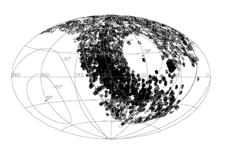
Recently, we have applied the LSS-GAC flux calibration pipeline as well as Version 2 of the parameter determination pipeline LSP3 used to generate the LSS-GAC DR2 to all spectra of the LAMOST Galactic surveys collected by June, 2016. Basic stellar parameters, $V_{\rm r}$, $T_{\rm eff}$, $\log\,g$ and [Fe/H] yielded by the default LAMOST pipeline LASP, have been publicly released in December 2016 in the LAMOST DR4. Results from the LSP3 lead to a value-added catalog containing parameters derived from a total of 6.5 million stellar spectra of SNRs higher than 10, for 4.4 million unique stars. The database is used to define the MSTO and sub-giant star sample in the current work. Fig. 1 plots the spatial distribution of stars in this value-added catalog.

2.2. Choice of effective temperatures

Figure 2.— Differences of LSP3 spectroscopic estimates of $T_{\rm eff}$ and the photometric values deduced from the color-metallicity-temperature relations of Huang et al. (2015), plotted against the photometric $T_{\rm eff}$ (left) and the spectroscopic (i.e. LSP3) [Fe/H] (middle). The upper panels show the LSP3 results based on the weighted-mean method, while the lower panels show those with the LSP3 KPCA method. Histogram of the differences, as well as Gaussian fits to the histograms are shown in the right panels. Means and 1-$\sigma$ dispersions of the Gaussians are marked in the plots.

Figure 3.— Color-coded stellar number density distributions (in 10-based logarithmic scale) in the $T_{\rm eff}$–${\rm M}_{V}$ plane for stars in three [Fe/H] bins. Y² isochrones of ages 1, 2, 4, 6, 10 and 14 Gyr are over-plotted. The top and middle panels show LSP3 estimates of $T_{\rm eff}$ with the weighted-mean and the KPCA method, respectively. The bottom panels show the same as the middle panels, except that the over-plotted isochrones have been calibrated to the temperature scale of Huang et al. (2015).

Figure 4.— Differences of temperature scales of Casagrande et al. (2010) and Huang et al. (2015) as a function of $T_{\rm eff}$ for different [Fe/H].

Accurate estimates of $T_{\rm eff}$ are essential for age estimation, particularly for avoiding significant biases and systematic errors in the results. There are two sets of $T_{\rm eff}$ estimates in the value-added catalog, both estimated using the MILES empirical spectral template library (Sánchez-Blázquez et al., 2006) but with two different algorithms, the weighted-mean and the kernel-based principal component analysis (KPCA). Note that values of $T_{\rm eff}$ of the MILES template stars have been re-calibrated using the color-temperature-metallicity relation of Huang et al. (2015), which is derived based on stars with direct, interferometric angular diameter measurements and Hipparcos parallaxes. The weighted-mean method works straight-forwardly with well controlled results, and yields robust $T_{\rm eff}$ estimates, even for a spectral SNR as low as 10 (Xiang et al., 2015a, 2017b). On the other hand, due to the inhomogeneous distribution of the MILES stars in the parameter space, the weighted-mean estimates of $T_{\rm eff}$ suffer from the so-called clustering effects, at the level of a few tens to a hundred Kelvin. While estimates of $T_{\rm eff}$ yielded by the KPCA method do not suffer from significant clustering effects, the robustness of the results rely heavily on the SNRs of spectra under analysis (Xiang et al., 2017a).

Since no direct external calibration of $T_{\rm eff}$ has been carried out for LSS-GAC DR2, some further examinations of the $T_{\rm eff}$ estimates are desirable, especially considering that there could be some potential offsets in absolute scale between temperatures inferred from the color-temperature-metallicity relation of Huang et al. (2015) and those of the theoretical isochrones. For this purpose, here we first define a photometric sample from the value-added catalog. We select stars with photometric errors smaller than 0.03 mag in SDSS $g$ and $r$-bands, and with errors smaller than 0.04 mag in 2MASS $K_{\rm s}$ band. We require the interstellar reddening $E(B-V)$ retrieved from the map of Schlegel, Finkbeiner & Davis (1998, hereafter SFD98) to have a value smaller than 0.05 mag and that derived from the star-pair method in the value-added catalog to be smaller than 0.1 mag, considering that for stars near the Galactic plane the SFD98 map sometimes yields too small, unrealistic values. We further require the stars to have a distance larger than 300 pc as the SFD98 may have overestimated the reddening of stars of shorter distances. Stars observed with bad fibers of low throughputs or stars potentially affected by fiber crosstalk are discarded by requiring ${\rm BADFIBER}=0$ and ${\rm SNR-BRIGHTSNR}>-150$. Here ‘BRIGHTSNR’ is the highest SNR of stars targeted by the 5 fibers adjacent to the fiber of the star of concern. Finally, we select only stars with a spectral SNR higher than 20. The above criteria lead to a total of 350,000 stars that form our photometric sample.

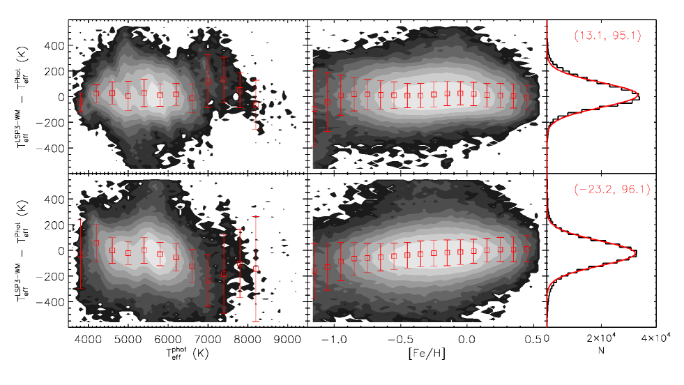
Fig. 2 plots the differences of LSP3 estimates of $T_{\rm eff}$ and photometric values inferred from $g-K_{\rm s}$ colors using the relation of Huang et al. (2015), as a function of $T_{\rm eff}^{\rm phot}$ or [Fe/H]. Here the $g-K_{\rm s}$ colors are dereddened using SFD98 values of $E(B-V)$ and the extinction coefficients of Yuan, Liu & Xiang (2013). The figure shows that for the temperature range 3800–6300 K, $T_{\rm eff}$ values yielded by both the weighted-mean and the KPCA methods are in good agreement with the photometric values, with differences $<50$ K. At higher temperatures, the KPCA method yields values that are smaller than the photometric ones by 100–200 K, while the weighted-mean method yields results that are higher than the photometric values by 150 K for stars around 7000–7500 K. No systematic trends of differences with [Fe/H] are seen for $T_{\rm eff}$ yielded by the weighted-mean method in the [Fe/H] range $-1.0$ – 0.5 dex, the applicable metallicity range of the color-metallicity-temperature relation of Huang et al. (2015). However, for $T_{\rm eff}$ estimated with the KPCA method, there is a positive trend of difference with [Fe/H]. Nevertheless, the dispersions of the differences amount to only $\sim$95 K for both sets of LSP3 temperature estimates. Considering that a bias in $T_{\rm eff}$ estimates, especially a positive trend of $T_{\rm eff}$ with [Fe/H] may lead to some undesired systematics in the age estimates and in the distribution of stars in the age–metallicity space, we choose to correct for the biases, albeit small, in the KPCA $T_{\rm eff}$ estimates. The correction is done in the $T_{\rm eff}$–[Fe/H] plane by interpolating a grid of bias values created with the photometric sample.

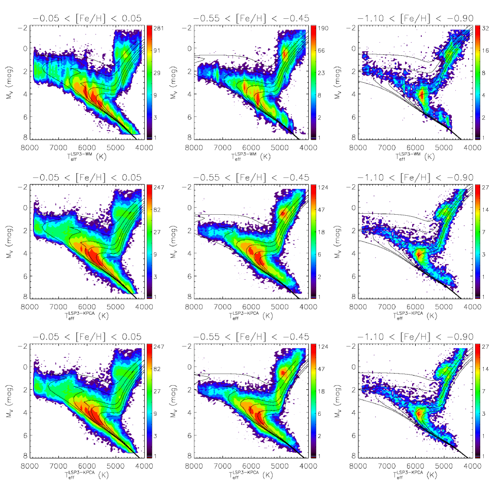
Fig. 3 plots the logarithmic (base 10) number density of stars in the $T_{\rm eff}$ – ${\rm M}_{V}$ diagrams for three metallicity bins. To better illustrate the potential systematic patterns, only stars with spectral SNRs higher than 50 are shown. The Yonsei-Yale (Y²; Demarque et al., 2004) isochrones are overplotted. The figure shows that for stars of solar metallicity bin, the distribution in the $T_{\rm eff}$ – ${\rm M}_{V}$ diagram is basically consistent with isochrones. In contrast, for stars in the two metal-poor bins, the distributions deviate from the theoretical isochrones. For example, most (88 per cent) stars of ${\rm M}_{V}>4.0$ mag in the $-1.0<{\rm[Fe/H]}<-0.9$ dex bin have temperatures of about 200 K lower than values of the isochrones of 14 Gyr, older than the dynamic age of the universe (13.8 Gyr, e.g. Planck Collaboration et al., 2016). The offsets are significant and can not be caused by random errors of the stellar parameters only. The apparent [Fe/H]-dependent inconsistencies are undesired and could have severe impacts on our sample selection, age estimates and subsequently statistical analysis. Similar deviates are seen when the isochrones of the Dartmouth Stellar Evolution Database (DESP; Dotter et al., 2008) or the PAdova and TRieste Stellar Evolution Code (PARSEC; Bressan et al., 2012) are used. We suspect that the offsets are caused by different temperature scales of the color-temperature-metallicity relation of Huang et al. (2015) and the theoretical isochrones. The color-temperature-metallicity relation of Huang et al. (2015) is based on ‘directly’ measured temperatures, while the values of $T_{\rm eff}$ of theoretical isochrones depend on the stellar atmospheric models adopted. The figure also shows that, as mentioned above, values of $T_{\rm eff}$ yielded by the weighted-mean method suffer moderate clustering effects. In the current work, we thus adopt the KPCA estimates of $T_{\rm eff}$ in order to avoid any potential patterns in the age estimates due to the clustering effect in the temperature estimates.

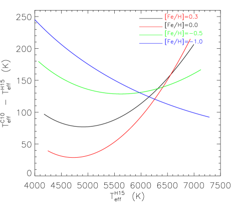
It is of particular interest to unravel the causes of the [Fe/H]-dependent discrepancies of temperature scales between the direct measurements and the theoretical isochrones, as it may help understand the robustness of those currently widely used stellar atmospheric models, especially those of metal-poor stars. In fact, regardless of [Fe/H], Huang et al. (2015) have found an overall systematic difference of about 100 K between the temperatures given by their photometric relations and those derived from methods based on the stellar atmospheric models in literature (e.g. Santos, Israelian & Mayor, 2004; Valenti & Fischer, 2005; Casagrande et al., 2010). This important issue is however out of the scope of this paper. As a temporary remedy to avoid potential biases in our age estimation, here we have opted to adjust the temperature scale of isochrones to match that of Huang et al. (2015). In doing so, we have implicitly assumed that the isochrone temperature scale is the same as that given by Casagrande et al. (2010) utilizing the infrared flux method (IRFM), which also relies on stellar atmospheric models. Fig. 4 plots the differences of IRFM $T_{\rm eff}$ of Casagrande et al. (2010) and those of Huang et al. (2015) for different metallicities. It is obvious that the differences depend on temperature and metallicity. At solar metallicity, the IRFM scale of Casagrande et al. (2010) gives $T_{\rm eff}$ that is $\sim$100 K higher than values yielded by the relation of Huang et al. (2015) for a temperature of $\sim$5800 K. The difference is consistent with the finding of Huang et al. (2015). However, the trends of differences with metallicity and temperature shown in the figure cannot be ignored for robust and unbiased age estimation. We correct the isochrone temperatures to match the scale of Huang et al. (2015) for each metallicity ${\rm[Fe/H]}>-1.2$ dex, but leave the more metal-poor isochrones untouched. The disposition will not yield any inconsistency in our results because in the current work we are concerned only with disk stars of ${\rm[Fe/H]}>-1.0$ dex, and most of our sample stars have [Fe/H] higher than $-0.8$ dex. Nevertheless, we have carefully examined the age estimation for stars of low metallicities. A test shows that if we instead calibrate the LSP3 spectroscopic temperatures to match the IRFM scale and estimate the ages using the isochrones without temperature corrections, the resultant ages do not deviate from the current estimates by any significant amounts ($<1$ Gyr). Note that the IRFM temperature scale of Casagrande et al. (2010) is only applicable to a limited color range ($0.78<V-K_{\rm s}<3.15$). To overcome the limitation, the isochrone grids of hotter temperatures are corrected for using the amount of temperature corrections at the boundary. This simplification again will not cause any significant impact in our results as hot ($T_{\rm eff}>7000$ K) stars are young ($\lesssim$1 Gyr) and a 100–200 K difference in temperature will cause only very small changes in the age estimates. Finally, we have to point out that the IRFM temperature scale of Casagrande et al. (2010) is only appropriate for dwarf and subgiant stars but not for giant stars. Since we focus our work on MSTO and subgiant stars, this limitation does not affect the current work.

The bottom panels of Fig. 3 compare the data and the isochrones after the temperature corrections. The plots show much better agreement, not only for the metal-poor bins, but also for the solar-metallicity bin. Most of the MSTO stars are now encompassed by 14 Gyr isochrones. Nevertheless, for the metal-poor, low-temperature ($T_{\rm eff}\lesssim 5300$ K) main sequence stars, there are still some discrepancies between the data and the isochrones. Those offsets could either be due to possible different temperature scales of the isochrones and the IRFM calibration of Casagrande et al. (2010), or caused by overestimates of isochrone absolute magnitudes for those metal-poor, low-temperature stars. However, these remaining discrepancies are not expected to have any significant impact on our results because we focus on MSTO and subgiant stars, and our target selection criteria ($\S{3}$) have effectively excluded those cool, metal-poor main sequence stars.

3. sample selection

Figure 5.— Example of sample selection criteria in the $T_{\rm eff}$–${\rm M}_{V}$ diagram for the solar metallicity bin. The background grey scale map shows the number density (in 10-based logarithmic scale) of stars of $-0.05<{\rm[Fe/H]}<0.05$ dex in the value-added catalog. Blue curves, from left to right, are Y² isochrones of ages ranging from 1 to 16 Gyr for [Fe/H]=0.0 and [$\alpha$/Fe] = 0.0 dex. Stars falling within the two red curves constitute the main sequence turn-off and subgiant sample stars for this solar metallicity bin.

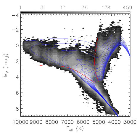
We define a sample of MSTO and subgiant stars for which reliable stellar ages can be determined via isochrone fitting. In doing so, we first trace the locus of MSTO in the $T_{\rm eff}$ – ${\rm M}_{V}$ plane using the Yonsei-Yale (Y²) isochrones, similar to the technique of Xiang et al. (2015b) except in the latter case the analysis was carried out in the $T_{\rm eff}$ – log $g$ plane instead. This is done for isochrones with [Fe/H] from $-3.0$ dex to $+0.5$ dex with a step of 0.1 dex. For each [Fe/H], an [$\alpha$/Fe] value is adopted, which increases from 0.0 dex for ${\rm[Fe/H]}\geq 0.0$ dex to 0.3 dex for ${\rm[Fe/H]}\leq-1.0$ dex. Similarly, the trajectory of the base of red giant branch (RGB) is also determined in the $T_{\rm eff}$ – ${\rm M}_{V}$ plane. Let ${\rm M}_{V}^{\rm TO}$, a function of $T_{\rm eff}$, denote the trajectory of the MSTO, and $T_{\rm eff}^{\rm bRGB}$, a function of ${\rm M}_{V}$, denote the trajectory of the base of RGB. The sample stars are then defined by requiring,

$$T_{\rm eff}>T_{\rm eff}^{\rm bRGB}+\Delta{T_{\rm eff}},$$ (1)

$${\rm M}_{V}<{\rm M}_{V}^{\rm TO}+\Delta{\rm M}_{V},$$ (2)

where $\Delta{T_{\rm eff}}$ is set to reduce contamination from RGB stars due to the errors in $T_{\rm eff}$ estimation, and is set to be a constant of 300 K. $\Delta{\rm M}_{V}$ is set to be a function of $T_{\rm eff}$: $\Delta{\rm M}_{V}=0.0005\times(T_{\rm eff}-T_{\rm eff}^{\rm MINISO})$, where $T_{\rm eff}^{\rm MINISO}$ is the minimum temperature of MSTO of isochrones for a given set of [Fe/H] and [$\alpha$/Fe]. Fig. 5 plots an example of the criteria for [Fe/H] = 0 and [$\alpha$/Fe] = 0 dex. Our choice of $\Delta{\rm M}_{V}$ ensures that main sequence stars of high temperature (e.g. $>6500$ K) are also included in our sample, as their ages can be well-estimated. Note that trajectories of the MSTO and base RGB in the $T_{\rm eff}$ – ${\rm M}_{V}$ plane, as well as the adopted $T_{\rm eff}^{\rm MINISO}$, for different metallicities are listed in the Appendix.

To select sample stars from the value-added catalog, we first discard stars of saturated spectra, by requiring ${\rm SATFLAG}=0$, stars potentially suffering from significant fiber cross-talking, by requiring ${\rm SNR-BRIGHTSNR}>-150$, and stars observed with bad fibers, by requiring ${\rm BADFIBER}=0$. For stars with duplicate observations, only results based on the spectrum of highest SNR are selected. Results of unique stars are then grouped into [Fe/H] bins of width 0.1 dex. MSTO and subgiant sample stars of the individual metallicity bins are then selected using the criteria defined by Eqs. (1) and (2). To reduce potential contamination from giant and supergiant stars, as well as to ensure the robustness of stellar parameters used to defined the sample, we require that the sample stars must have $T_{\rm eff}<10000$ K, log $g>3.0$ dex, ${\rm[Fe/H]}>-1.0$ dex and a spectral SNR higher than 20. Note that several sets of stellar parameters are provided in the value-added catalog. The parameters adopted here refer to the recommended ones. The [Fe/H] cut above is used to discard metal-poor halo stars, whose LSP3 stellar parameters may need some further improvement, and thus to leave us with a pure disk star sample. Finally, for each metallicity bin, stars that stray into the area in the $T_{\rm eff}$ – ${\rm M}_{V}$ plane beyond the boundary defined by isochrones of age 16 Gyr towards the direction of lower temperatures, are discarded. With the above criteria, a total of 932,313 unique MSTO and subgiant sample stars are selected. Here and later, we use the term ‘MSTO-SG stars’ to denote those selected MSTO and subgiant stars for convenience. We note that there are 420,000 duplicate observations of these MSTO-SG stars in the value-added catalog.

Figure 6.— From upper-left to bottom right are respectively the distribution of $r$-band magnitudes, the cumulative percentage distribution of spectral SNRs, the distribution of [Fe/H], errors of ${\rm M}_{V}$ estimates as a function of SNR, the distributions of distances and distance errors, of the MSTO-SG star sample.

Fig. 6 plots the distributions of $r$-band magnitudes, SNRs, [Fe/H], ${\rm M}_{V}$, distances and distance errors of the MSTO-SG sample stars. The stars have $r$-band magnitudes ranging from 9 to 18 mag, peaking at $\sim$14 mag. This is owning to the large number of very bright stars of $r<14$ mag observed utilizing the grey/bright lunar nights. The sample stars cover a wide range of spectral SNRs, and about 60 per cent of the stars have a SNR higher than 50. The [Fe/H] distribution peaks at about $-0.1$ dex, and less than 2 per cent of the stars are more metal-poor than $-0.8$ dex. Errors of ${\rm M}_{V}$ estimates are sensitive to the SNR, with typical values of 0.7 mag for a SNR of 20, and decrease to 0.25 mag at SNRs$\gtrsim 80$. The median value of ${\rm M}_{V}$ errors of the whole sample stars is 0.37 mag. About half of the stars have a distance smaller than 1.2 kpc, and about a quarter more distant than 2 kpc. The fraction of stars more distant than 3 kpc is 11 per cent. The median value of the relative distance errors is 16.8 per cent, with 38 per cent of the stars having a relative distance error smaller than 15 per cent, and 21 per cent having a relative distance error larger than 25 per cent.

4. Method

Stellar age and mass are estimated via matching the observed stellar parameters with theoretical isochrones with a Bayesian scheme similar to that of Jørgensen & Lindegren (2005). The stellar parameters include $T_{\rm eff}$, ${\rm M}_{V}$, [Fe/H] and [$\alpha$/Fe]. Note that although the value-added catalog also provides estimates of ${\rm M}_{K_{\rm s}}$, here we have opted not to use both ${\rm M}_{V}$ and ${\rm M}_{K_{\rm s}}$ for the age estimation because $M_{\rm V}$ and ${\rm M}_{K_{\rm s}}$ are found to be largely correlated with each other. Similarly, log $g$ is not used because it carries largely the same information as $M_{\rm V}$ considering that the log $g$ values of template/training stars used by LSP3 for log $g$ estimation are constrained mainly by the Hipparcos parallaxes, i.e., the same as those used for the estimation of absolute magnitudes. Including ${\rm M}_{K_{\rm s}}$ and log $g$ in the age estimation might in principle help constrain the results, but this works only if the above correlations can be dealt with properly, and we intend to leave this to a future work. The value-added catalog provides also two sets of [$\alpha$/Fe] estimates for MSTO-SG stars, one ([$\alpha$/Fe]₁) utilizing spectra of 3910–3980, 4400–4600 and 5000–5300 Å, the other ([$\alpha$/Fe]₂) utilizing 4400–4600 and 5000–5300 Å only (cf. Xiang et al., 2017b). Considering that the inclusion of 3910–3980Å may cause artifacts for low temperature stars as the Ca ii H, K lines are usually saturated, and also that the [$\alpha$/Fe]₁ are found to exhibit larger random errors for high temperatures ($\gtrsim 6000$ K) stars, we choose to use [$\alpha$/Fe]₂ throughout the paper if not specified.

4.1. Stellar isochrones

We have chosen to use the Yonsei-Yale (${\rm Y}^{2}$) isochrones (V2; Demarque et al., 2004) for the age estimation. The ${\rm Y}^{2}$ isochrones cover a wide range of stellar ages (0.001–20 Gyr), which is convenient for us to apply a Bayesian algorithm as biases induced by the abrupt age cutoff of the isochrone grids could be negligible. Moreover, the ${\rm Y}^{2}$ isochrones have grids of different [$\alpha$/Fe], allowing us to make use of the [$\alpha$/Fe] measurements to better constrain the ages. Grids of the ${\rm Y}^{2}$ isochrones are interpolated into a uniform set of grids of step 0.1 dex in [Fe/H] and [$\alpha$/Fe], 0.1 Gyr in age for ${\rm age}<1$ Gyr, 0.2 Gyr for $1<{\rm age}<2$ Gyr and 0.5 Gyr for ${\rm age}>2$ Gyr, utilizing the interpolator provided by Demarque et al. (2004). The isochrones adopt the color table of Lejeune, Cuisinier & Buser (1998) and assign colors and magnitudes in $UBVRIJHKLL^{\prime}M$ photometric bands for each grid model. Here the $UBV$ system is that of Buser (1978), of which the $V$-band agrees well with the Johnson (e.g. Bessell, 2005), $RI$ that of Bessell (1979), and $JHKLL^{\prime}M$ that of Bessell & Brett (1988).

There are also quite a few other sets of stellar isochrones that are widely used, such as the Dartmouth Stellar Evolutionary Database (DSEP; Dotter et al., 2008) and the PAdova and TRieste Stellar Evolution Code (PARSEC; Bressan et al., 2012). Different isochrones are based on more or less different stellar model assumptions, and thus may lead to some different age estimates. Generally, the different isochrones yield stellar ages for MSTO stars with some systematic differences of the order of about 1 Gyr, along with dispersions at the same level (e.g. Haywood et al., 2013; Xiang et al., 2015b; Hills et al., 2015).

4.2. Age and mass estimation

The observed properties of a star are largely determined by three parameters, namely age ($\tau$), initial stellar mass ($M$) and chemical compositions ($Z$). In Bayesian theory, their joint (posterior) probability density function thus can be written as,

$$f(\tau,M,Z)=Af_{0}(\tau,M,Z)L(\tau,M,Z),$$ (3)

where $f_{0}$ is the priori density distribution, $L$ is the likelihood function, and $A$ is a normalization factor to ensure $\int\int\int f(\tau,M,Z){\rm d}\tau{\rm d}M{\rm d}Z=1$.

Let $\mathbf{O}$ denote the observed stellar parameters $T_{\rm eff}$, ${\rm M}_{V}$, [Fe/H], [$\alpha$/Fe], and $\mathbf{P}$ denote the isochrone values given $\tau$, $M$ and $Z$. The likelihood function $L$ is then given by,

$$L(\tau,M,Z)=\prod_{i=1}^{n}\frac{1}{\sqrt{2\pi}\sigma_{i}}\times\exp\left(-\frac{\chi^{2}}{2}\right),$$ (4)

$$\chi^{2}=\sum_{i=1}^{n}\left(\frac{O_{i}-P_{i}(\tau,M,Z)}{\sigma_{i}}\right)^{2},$$ (5)

where $n$ is the number of observables, and $\sigma_{i}$ is the Gaussian error of the $i$-th observed parameter.

For the priori density distribution, we adopt the same formula as used by Jørgensen & Lindegren (2005),

$$f_{0}(\tau,M,Z)=\psi(\tau)\phi(Z\mid\tau)\xi(m\mid Z,\tau).$$ (6)

Here $\psi(\tau)$ is the star formation history, $\phi(Z\mid\tau)$ is the metallicity distribution as a function of age, and $\xi(m\mid Z,\tau)$ is the initial mass function (IMF) as a function of metallicity and age. In principle, the distributions of $\psi(\tau)$ and $\phi(Z\mid\tau)$ should be a function of position across the Milky Way. Considering that the star formation rate and the metallicity distribution as a function of age as well as of spatial position, are not well known, we have adopted a flat distribution for both $\phi(Z\mid\tau)$ and $\xi(m\mid Z,\tau)$ to avoid potentially large biases in the resultant age estimates. The IMF is better known – the star formation process yields more low mass stars than massive stars and the number of stars as a function of mass can be generally well described by power-laws or log-normal (e.g. Salpeter, 1955; Kroupa, 2001; Chabrier, 2003). Here we have adopted the IMF form of Kroupa (2001),

$$\xi(m)\propto m^{-a},$$ (7)

where $a=0.3$ for $m<0.08M_{\odot}$, $a=1.3$ for $0.08<m<0.5M_{\odot}$ and $a=2.3$ for $m>0.5M_{\odot}$. We assume that the IMF is invariant with age and metallicity. For Galactic field stars, this may not be a bad assumption (e.g. Kroupa, 2001; Kroupa et al., 2013), especially considering that our sample stars cover a rather limited mass range.

For each age, the joint probability is then evaluated using the isochrones grids with parameter values within $\pm$3$\sigma$ of the observed ones, and the age of the star of concern is then estimated by taking the mean of the distribution with error given by the standard deviation. An alternative age estimate is obtained by taking the mode of the joint probability distribution. In the latter case, the error of age is estimated by requiring that the 1$\sigma$ error covers 68% of the area of the joint probability distribution. In some cases where the parameters are poorly estimated, the resultant joint probability has a broad distribution, peaking either near the young or old age cutoffs of the isochrones. As a consequence, the resultant mean ages tend to fall by the middle of the age interval of the isochrones, while the mode ages tend to have a value close to the upper or lower boundary of the age interval. A comparison of the two age estimates helps one to evaluate the quality of age estimation. Such cases do not occur often, as most of our sample stars have well determined parameters that fall within the suitable range of age estimation. The mean ages thus derived are analyzed in the Sections below. The mass estimate is also taken as the weighted-mean value given by all isochrone grids within $\pm$3$\sigma$ of the observed stellar parameters. Here the weights for mass estimates are the same as those for the age estimates. Note that for both age and mass estimation, effects from unevenly spaced age grids have been considered via multiplying the joint probability by $\Delta\tau$, age space of the grids.

[$\alpha$/Fe] of the Y² isochrone grids is limited in the range of 0.0–0.6 dex. As many stars have [$\alpha$/Fe] values close to or smaller than 0.0 dex, an [$\alpha$/Fe] cutoff of the isochrones causes a cutoff in the joint probability distribution function, which induce bias in the age and mass estimates. To avoid such bias, we opt not to use [$\alpha$/Fe] when calculating the joint probability. Instead, we calculate ages for isochrones of [$\alpha$/Fe] values of 0.0, 0.2 and 0.4 dex separately, and then estimate the final age by linearly extrapolating (interpolating for stars with [$\alpha$/Fe] between 0 and 0.4 dex) the results to match the observed [$\alpha$/Fe].

5. validation of age and mass estimates

5.1. Test with mock data

Figure 7.— Differences of estimated and true ages as a function of the latter (upper) and former (lower) for the mock sample. The color-coded contours show stellar number densities in logarithmic (base 10) scale. Mean and standard deviations of differences for the individual age bins are shown by dots with error bars.

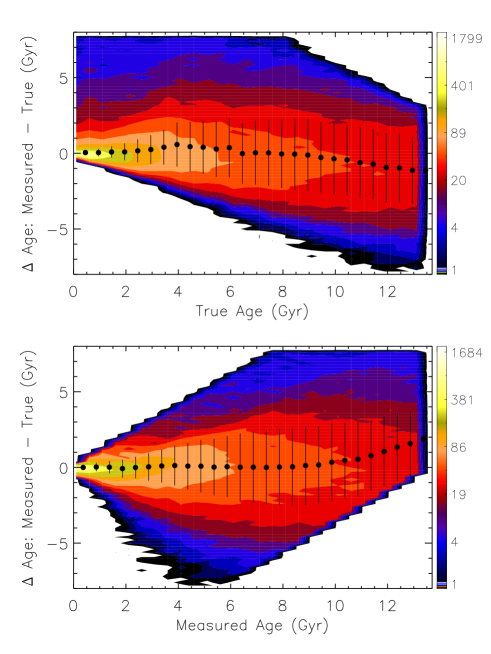
As an examination of the method, we estimate stellar age and mass for a mock data set generated with Monte-Carlo simulation, and compare the results with true values. To generate the mock data, 35 sets of isochrones are first selected, each with a given combination of $\tau$, [Fe/H], [$\alpha$/Fe]. The isochrones cover an age range of 0.2–13.5 Gyr, with a step of 0.2 and 0.5 Gyr respectively for isochrones of ages below and above 1 Gyr. The isochrones cover an [Fe/H] range of $-1.8$–0.3 dex and an [$\alpha$/Fe] range of 0.0–0.4 dex, with the older, more metal-poor isochrones having higher [$\alpha$/Fe] values. For each set of isochrones, mock stars for a total mass of 50000 $M_{\odot}$ are retrieved following the IMF of Kroupa (2001). Gaussian errors are added to the retrieved $T_{\rm eff}$, ${\rm M}_{V}$ and [Fe/H], with dispersions of 130 K, 0.4 mag, and 0.15 dex, respectively. Note that these values of dispersions correspond to typical, not minimum, errors of the MSTO-SG sample stars.

Figure 8.— $Left$: Distributions of estimated ages for stars of given true ages marked by the vertical red lines in the individual panels. Values of the true age, as well as the percentage difference and standard deviation are marked. $Right$: Same as left, but for distributions of true ages for stars of estimated ages in a limited ($\pm 0.25$) range.

Figure 9.— Comparison of measured and true masses for the mock data set. The mean and dispersion of a Gaussian fit to the differences are marked in a plot on the right.

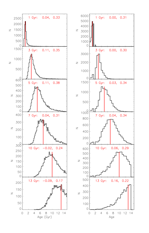
MSTO and sub-giant stars are selected from the mock catalog, and their ages and masses are estimated with the Bayesian method described above. Fig. 7 plots the differences of measured and true ages as a function of either the former or the latter. The figure shows that the mean differences are close to zero at all ages except for the oldest stars. Ages of truely oldest ($>12$ Gyr) stars are systematically underestimated by $\sim$1 Gyr, while stars of oldest measured ages are in fact generally 1–2 Gyr younger. The standard deviations of the differences increase from $\sim$0.6 Gyr at age 2 Gyr to 2.3 Gyr at age 8 Gyr, then flatten. There are a small fraction of young stars whose ages are significantly overestimated and a small fraction of old stars whose ages are significantly underestimated due to their large parameter errors. As a result, for stars of measured ages between approximately 4 and 9 Gyr, their true ages may spread over a wide range, although the number of stars having large age errors is expected to be small. Fig. 8 plots one-dimensional distribution of the measured ages for stars with the same true age, as well as distribution of the true ages for stars within a given range of measured age. For a given true age, the distribution of measured ages is clearly non-Gaussian but exhibits a tail at the older end, a consequence of the uneven distribution of isochrones in the $T_{\rm eff}$ – ${\rm M}_{V}$ plane. Stars of the oldest measured ages show a tail of small values in the distribution of their true ages, mainly caused by the cutoff of true age of isochrones at 13.5 Gyr. Typical percentage values of the mean differences are a few per cent, with typical standard deviations of 25 per cent for old stars and 35 per cent for young stars.

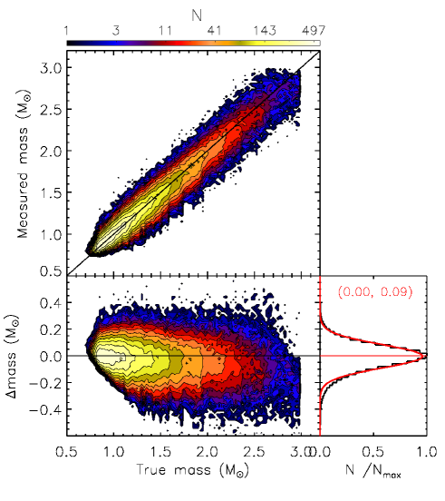
Fig. 9 plots a comparison of estimated and true masses. The figure shows very good consistency, with small systematic differences ($<0.05$ $M_{\odot}$) for mass range 0.7–3.0 $M_{\odot}$, along with standard deviations only $\sim$ 0.09 $M_{\odot}$, indicating typical relative mass errors smaller than 10 per cent.

Similar analyses were carried out for other sets of parameter errors corresponding to MSTO-SG sample stars having different spectral SNRs. For example, for parameter error set of 150 K, 0.5 mag, 0.15 dex for respectively $T_{\rm eff}$, ${\rm M}_{V}$ and [Fe/H], the results show that the standard deviations of age differences between the measured and true values are only slightly ($\lesssim$5 per cent) increased compared to the above quoted values. For the parameter error set of 100 K, 0.3 mag, 0.1 dex, which correspond to spectral SNRs$\gtrsim$60, the standard deviations are only 20 per cent for old stars, and 25 per cent for young stars. This is encouraging since more than one third of the sample stars have parameter errors smaller than these values.

5.2. Comparing age and mass estimates with seismic values

Figure 10.— Comparison of ages estimated using the approach of the current work and those derived based on the asteroseismic log $g$.

Figure 11.— $Left$: Comparison of mass estimates in the current work and those of Huber et al. (2014, black circles) and those deduced from the asteroseismic scaling relation (red circles). A Gaussian fit to the differences yields a mean and dispersion of $0.02$ and 0.11 $M_{\odot}$, respectively.

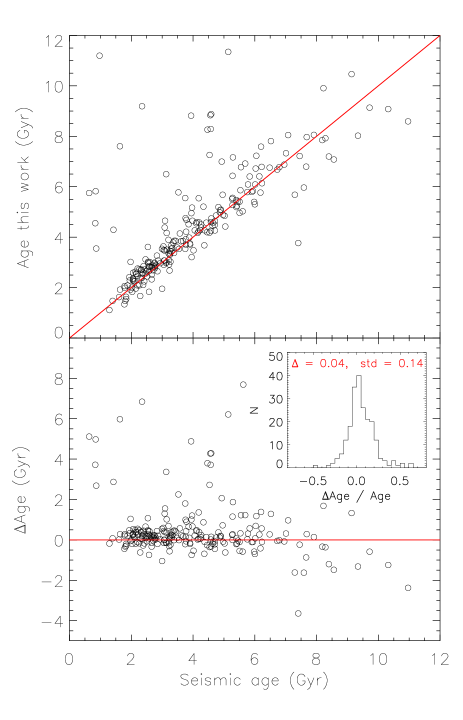
Stellar asteroseismology is suggested to yield log $g$ with uncertainties smaller than 0.05 dex (e.g. Creevey et al., 2013; Hekker et al., 2013; Chaplin et al., 2014). We thus expect that stellar ages derived from asteroseismic log $g$ are more accurate than – and therefore can be used to test – the current estimates. For our sample, 230 stars have asteroseismic log $g$ measurements available from the catalog compiled by Huber et al. (2014). For those stars, we have determined their ages using the asteroseismic log $g$ measurements along with our spectroscopic estimates of $T_{\rm eff}$, [Fe/H] and [$\alpha$/Fe]. Fig. 10 compares ages estimated using ${\rm M}_{V}$ (‘Age of this work’) with those based on the asteroseismic log $g$ measurements. The figure shows good consistency between the two sets of age estimates. The mean value of percentage differences for the whole sample is quite small, along with a standard deviation that is only 14 per cent. Nevertheless, for old stars, ages estimated using the approach of the current work tend to be underestimated by $\sim$1 Gyr compared to values derived with the asteroseismic log $g$, consistent with results shown in Fig. 7 for the mock data set. There is also a small fraction of stars for which the current age estimates are significantly larger than the asteroseismic log $g$ based estimates. Some of these stars are likely subgiant or red clump stars whose absolute magnitudes and effective temperatures from the LAMOST spectra are over-estimated. Note that for both sets of age estimates, the same set of parameters $T_{\rm eff}$, [Fe/H] and [$\alpha$/Fe] are used, so the differences seen in Fig. 10 reflect the errors induced by the uncertainties in ${\rm M}_{V}$ only.

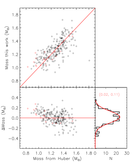
Fig. 11 compares our mass estimates with those of Huber et al. (2014) for the 230 common stars, as well as with stellar masses directly inferred from the asteroseismic scaling relation for a subset sample of 17 stars whose scaling relation based masses have a propagated random error smaller than 0.2 $M_{\odot}$. $T_{\rm eff}$ adopted in this work is used for inferring masses from the scaling relation. Masses of Huber et al. are derived using asteroseismic log $g$, photometric $T_{\rm eff}$ and [Fe/H] utilizing multiple evolutionary tracks, but mainly the DESP tracks. Interestingly, although different sets of stellar parameters and isochrones have been used in deriving those stellar masses, the figure shows quite good agreement, with a mean difference of only 0.02 $M_{\odot}$ and a dispersion of 0.11 $M_{\odot}$. Nevertheless, at the high mass end, there is a subset of stars for which our current mass estimates are systematically lower by 0.25 $M_{\odot}$. Those stars are also the outliers found in Fig. 10. At the low mass end, it seems that the current estimates yield masses $\sim$0.1–0.2 $M_{\odot}$ larger. Similar result is also seen in the comparison with masses derived from the scaling relation. For those stars, duplicate observations of LAMOST, as well as an examination of ${\rm M}_{V}$ values derived using parallaxes from the Tycho-Gaia astrometric solution (TGAS; Michalik, Lindegren & Hobbs, 2015; Lindegren et al., 2016), suggest that our current estimates are robust. We thus suspect that the discrepancies are probably caused by random errors in asteroseismology based mass estimates or by systematic errors in either the asteroseismic parameters or the asteroseismic scaling relation at the low mass end. In fact, for those low mass stars, masses inferred from scaling relation have a typical propagated error of $\sim$0.2$M_{\odot}$, which is significantly larger than the errors of our current mass estimates ($\sim$0.05 $M_{\odot}$).

5.3. Comparison with ages derived from the Tycho-Gaia parallaxes

Figure 12.— Comparison of age estimates of the current work and those derived utilizing absolute magnitudes inferred from the TGAS parallaxes.

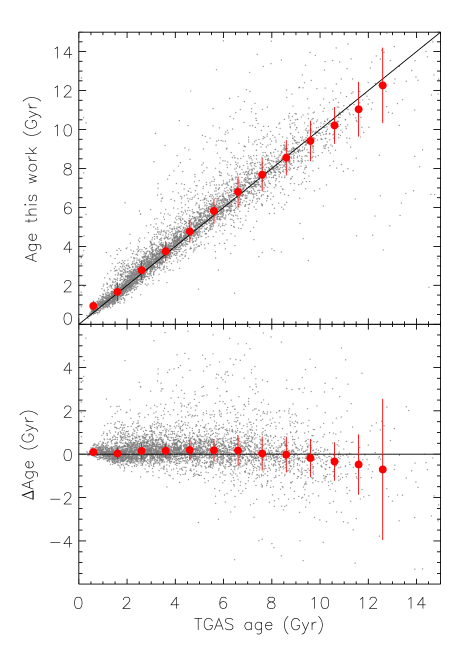
Accurate parallaxes from the Gaia TGAS catalog (Gaia Collaboration et al., 2016; Lindegren et al., 2016) provide independent determinations of absolute magnitudes and thus can be used to test our age estimates. A cross-identification of our value-added catalog with the TGAS catalog yields more than 0.3 million common stars, and about 50,000 of them have values of ${\rm M}_{V}$ inferred from the TGAS parallaxes with errors smaller than 0.2 mag. For those common stars, Xiang et al. (2017b) have compared values of ${\rm M}_{V}$ and distances with those derived utilizing the TGAS parallaxes, and found very good agreement. Here we further derive stellar ages using ${\rm M}_{V}$ inferred from the TGAS parallaxes and parameters $T_{\rm eff}$, [Fe/H] and [$\alpha$/Fe] from the value-added catalog to test the robustness of our age estimates.

After applying an error cut of 0.2 mag for ${\rm M}_{V}$ inferred from the TGAS parallaxes, 5258 unique stars in common with the TGAS catalog remain in our MSTO-SG star sample. Fig. 12 compares our age estimates for these MSTO-SG stars with ages estimated utilizing ${\rm M}_{V}$ inferred from the TGAS parallaxes. The figure shows good agreement, with a mean value of percentage differences close to zero and a standard deviation of only 14 per cent. Similar to the results shown in Fig. 7 for the mock data, there is a small fraction of stars for which our results seem to be significantly overestimated, probably due to the large uncertainties of their atmospheric parameter and absolute magnitude estimates. Note that for both sets of age estimates, the same values of atmospheric parameters $T_{\rm eff}$, [Fe/H] and [$\alpha$/Fe] are used. So any discrepancies revealed by the comparison are likely mainly caused by the uncertainties in ${\rm M}_{V}$ estimates only.

5.4. Test with open clusters

Figure 13.— Comparison of age estimates of open clusters with literature values. The vertical error bars represent dispersions (standard deviations) of age estimates of the individual cluster member stars, while the horizontal error bars represent age estimates in literature.

Table 1Age estimates of open clusters.

Cluster	${\rm Age}_{\rm Liter}$	$\Delta{\rm Age}_{\rm Liter}^{a}$	Age	$\sigma$(Age)	[Fe/H]	$\sigma$[Fe/H]	$(m-M)_{0}$	$E(B-V)$	Number of starsb
	(Gyr)	(Gyr)	(Gyr)	(Gyr)
M35	0.15	0.1 – 0.2	0.7	0.5	$-0.14$	0.19	9.75	0.35	395 (217)
NGC2420	2.2	1.9 – 2.4	2.3	0.4	$-0.31$	0.09	11.70	0.04	34 (24)
M67	4.0	3.5 – 4.8	3.9	1.2	$-0.04$	0.08	9.80	0.03	982 (184)
Berkeley32	6.0	5.0 – 7.2	6.0	2.2	$-0.44$	0.10	12.44	0.21	18 (17)

^a

$References$ M35: von Hippel et al. (2002); Kalirai et al. (2003); Meibom, Mathieu & Stassun (2009);
NGC2420: Demarque, Sarajedini & Guo (1994); Twarog, Anthony-Twarog & Bricker (1999);
M67: Demarque, Green & Guenther (1992); Carraro et al. (1994); Dinescu et al. (1995); Fan et al. (1996); Richer et al. (1998); VandenBerg & Stetson (2004); Schiavon, Caldwell & Rose (2004); Balaguer-Núñez, Galadí-Enríquez & Jordi (2007); Sarajedini, Dotter & Kirkpatrick (2009); Barnes et al. (2016);
Berkeley32: Kaluzny & Mazur (1991); Richtler & Sagar (2001); Salaris, Weiss & Percival (2004); D’Orazi et al. (2006); Tosi, Bragaglia & Cignoni (2007).

^b

Including duplicate observations, and number of unique stars is shown in the brackets.

Open clusters in the Milky Way are generally believed to form from a monolithic gas cloud on short timescales, so that member stars of a cluster belong to a single-aged population. Ages of cluster members thus provide an independent test of the robustness of our age estimation. For this purpose, a number of LAMOST plates have been designed to target open clusters of different ages utilizing grey nights reserved for monitoring the instrument performance. Together with data from the main surveys, we are able to select MSTO-SG stars in four open clusters, namely M35 (NGC2168), NGC2420, M67 (NGC2682) and Berkeley32. These clusters cover an age range from $\sim$100 Myr to 6 Gyr.

A detailed description of member star identification for these open clusters will be presented elsewhere (Yang et al. in preparation). Brieflly, for M67 and Berkeley32, member stars are identified by combining LAMOST radial velocities and UCAC4 proper motions (Zacharias et al., 2013). For M35 and NGC2420, contaminations from background stars are so severe that kinematics alone is insufficient for robust member identification, so additional constrains from the distance moduli are used to discard background stars that deviate significantly ($>1.5$ mag) from the peak values of the clusters. The numbers of member stars that pass our selection criteria of MSTO-SG stars are listed in Table 1. Note that here we have excluded some blue stragglers that also pass our selection criteria of MSTO-SG stars but whose ages may have been significantly underestimated (cf. Section 7). The measured ages, metallicities, extinction values and distance moduli of the clusters, obtained by taking means of the individual member stars, as well as age estimates in the literature are also listed in Table 1.

Fig. 13 presents a direct comparison between the measured cluster ages and the literature values. The figure shows that our age estimates are largely in good agreement with the literature values, mostly derived by isochrone fitting of color-magnitude diagrams. The relatively large dispersion of ages of the individual member stars of Berkeley 32 is mainly due to the small number of member stars identified in this cluster. For the young open cluster M 35, the relatively large deviation of our estimate from the literature values is caused by net overestimates of stellar ages for individual ‘MSTO’ stars at low temperatures, as our sample selection criteria at low temperatures prefer both stars whose ${\rm M}_{V}$ are underestimated due to random errors and background MSTO stars with old ages.

5.5. Comparison of results from duplicate observations

Figure 14.— Differences of ages deduced from the duplicate and default observations. Different panels show results for stars in different SNR bins, as marked in the plots. Red dots and error bars show median values and standard deviations of the differences in the individual age bins.

Figure 15.— Same as Fig.14, but for mass estimates.

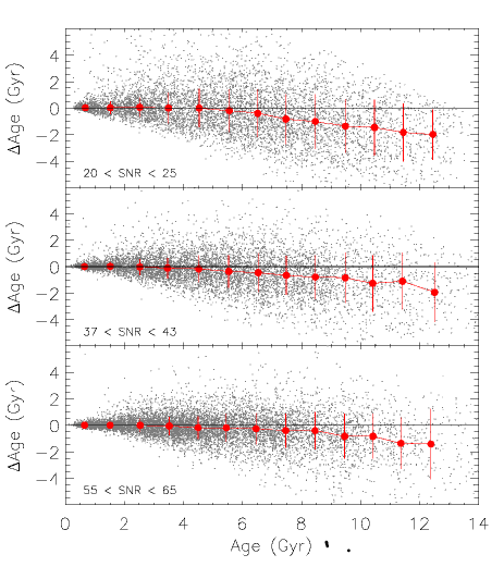
As mentioned in §3, there are more than 400,000 duplicate observations for the MSTO-SG sample stars. As a sanity check, Fig. 14 plots the differences of age estimates between those duplicate observations and the sample stars. Only duplicate observations that have SNRs comparable (within 20 per cent) to those of the sample stars are used in the comparison, and the comparisons are carried out for different SNR bins. The figure shows that for young (e.g. $<6$ Gyr) stars, the duplicate observations yield ages in excellent agreement with those deduced from the default observations. For old stars, duplicate observations yield ages 1–2 Gyr younger, depending on the SNRs. This deviation is due to the combination of the effects of the uneven distribution of the isochrones in the $T_{\rm eff}$–${\rm M}_{V}$ plane and errors in ${\rm M}_{V}$ estimates. As a result of the uneven distribution of the isochrones in the $T_{\rm eff}$–${\rm M}_{V}$ plane, deviation of the estimated ${\rm M}_{V}$ from the true value of an ‘exact’ MSTO star for a given effective temperature always yield underestimated age. The dispersions of the differences are small, generally less than 20 per cent at all ages. Note that both the default observations that define the sample and the duplicate observations contribute to the dispersions, and thus the random errors of ages estimated from the default observations as induced by the spectral noises are expected to be smaller than the dispersions (by a factor of $\sim 1.4$).

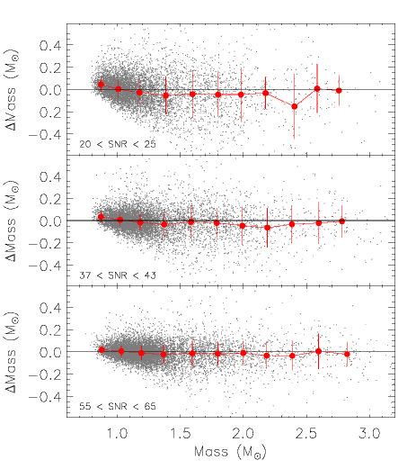
Fig. 15 plots the differences of masses estimated from the default and the duplicate observations. The agreement is quite good. Typical dispersions are a few to ten per cent, depending on the SNRs.

6. Properties of the sample

6.1. Distributions of ages and masses

Figure 16.— Distribution of ages and errors of the sample stars. The contours show stellar number densities in logarithmic (base 10) scale. The solid line delineates 40 per cent age errors, and the dashed lines, from left to right, show median errors as a function of age for stars within spectral SNR bins 20–25, 37.5–42.5 and 55–65, respectively.

Figure 17.— Distribution of median stellar ages in Galactic coordinate system ($l$, $b$). The data are divided into patches of 1.5^∘$\times$1.5^∘ to draw the map.

Figure 18.— Same as Fig. 16 but for mass estimates. The solid line delineates 10 per cent mass errors.

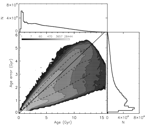
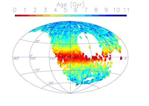
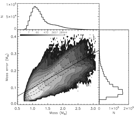
Fig. 16 plots the distributions of estimated ages and errors of the sample stars. The age distribution shows that there are more young stars than old ones in our sample. In particular, there is a peak of stars younger than 1 Gyr. Note that the distribution is a consequence of both the age distribution of the underlying stellar population and the selection effects of the observations as well as the sample definition, rather than simply the former. Both the observations and the SNR (at 4650Å) cut prefer young stars as they are bright and blue, and thus tend to have high SNRs. Our selection criteria used to define sample stars in the HR diagram also prefer young stars. A detailed analysis of the selection effects of the sample is quite complicated and out of the scope of the current paper. The errors of age estimates vary sensitively with the SNR. For stars of SNRs higher than 60, the relative errors of the age estimates are 20–25 per cent. For SNRs around 20, the values can be as large as 45 per cent or more. The median value of relative age errors for the whole sample is 34 per cent. The numerous young stars in the sample contribute a significant part of this number. If only stars older than 2 Gyr are considered, the number drops to 30 per cent. Fig. 17 shows the distribution of median stellar age in 1.5^∘$\times$1.5^∘ patches on the sky in Galactic coordinate system. As expected, the figure presents a clear positive age gradient with increasing Galactic latitudes. Median stellar ages in the disk of $|b|<10^{\circ}$ are younger than 2 Gyr, while at $|b|>50^{\circ}$, the median age becomes older than 7 Gyr.

The distributions of estimated masses and errors of the sample stars are shown in Fig. 18. The masses cover a range of 0.7–3.0 $M_{\odot}$, peaking at 1.1 $M_{\odot}$. Typical errors are smaller than a few per cent for low-mass stars ($<1.5$$M_{\odot}$), and about 10 per cent for more massive stars. The median value of the relative mass errors for the whole sample is 8 per cent.

6.2. Age distributions across the [Fe/H]–[$\alpha$/Fe] plane

Figure 19.— Distribution of median ages of stars in mono-abundance bins of 0.05 by 0.02 dex in the [Fe/H]–[$\alpha$/Fe] plane. The horizontal line delineates constant [$\alpha$/Fe] value of 0.0 dex.

Figure 20.— Percentile stellar number density in the [Fe/H]–[$\alpha$/Fe] plane for stars in different age bins, as labeled in red on the upper-right corner of the figures. The horizontal lines delineate constant [$\alpha$/Fe] values of 0.0 and 0.2 dex, respectively.

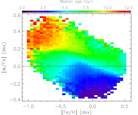
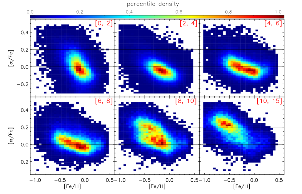
Fig.19 plots the median age of sample stars in the individual mono-abundance bins of the [Fe/H]–[$\alpha$/Fe] plane. To show potential patterns better, only stars of SNRs higher than 50 are used to generate the figure as their atmospheric parameters, especially [$\alpha$/Fe], are estimated with high quality. Since precisions of the [$\alpha$/Fe] estimates also vary significantly with effective temperatures, as hotter (younger) stars having less precisions due to weaker spectral features of [$\alpha$/Fe] indicators, we show results for stars of $T_{\rm eff}<6500$ K only in the figure. After the $T_{\rm eff}$ cut, it is found that there is still a few per cent of young ($\lesssim$4 Gyr) stars whose [$\alpha$/Fe] are artificially overestimated significantly ($>0.2$ dex), which may cause fake features in the [Fe/H]–[$\alpha$/Fe] patterns. Many of those stars are found to have weird spectra in the wavelength range used for the [$\alpha$/Fe] estimation (4400–4600 and 5000-5300Å), mainly due to artificial origin (e.g. contaminated by nearby bright stars, remains of cosmic ray removal etc.), but some are also due to intrinsic origin (e.g. composite spectra). An effort to identify those weird spectra automatically is still in progress. As a remedy, here and below we replace those [$\alpha$/Fe] by [$\alpha$/Fe]₁ provided in the value-added catalog, which is estimated using spectral wavelength range of 3910–3980, 4400–4600 and 5000-5300Å. Specifically, for stars with $T_{\rm eff}$ higher than 5800 K, if the [$\alpha$/Fe] has a value larger than [$\alpha$/Fe]₁ by 0.2 dex, then the [$\alpha$/Fe]₁ is adopted. The usage of [$\alpha$/Fe]₁ effectively reduces the number of young stars with significantly overestimated [$\alpha$/Fe].

Fig. 19 shows clear patterns in the distribution of median stellar ages across the [Fe/H]–[$\alpha$/Fe] plane. Generally, more metal-poor and $\alpha$-enhanced stars have older ages than metal-rich and $\alpha$-poor ones, consistent with previous findings of high resolution spectroscopy of solar-neighborhood stars (e.g. Haywood et al., 2013; Bergemann et al., 2014). The figure further reveals several interesting features. Firstly, the most metal-poor (${\rm[Fe/H]}<-0.5$ dex) and $\alpha$-enhanced (${\rm[\alpha/Fe]}>0.2$ dex) stars are dominated by stars older than 10 Gyr. Secondly, stars of intermediate-to-old ages (5–8 Gyr) show a contiguous distribution across the whole metallicity range from $-1.0$ to 0.5 dex, and exhibit a clear and sharp demarcation from younger and more $\alpha$-poor ([$\alpha$/Fe]$\lesssim 0.0$) stars. Thirdly, on the relatively $\alpha$-poor ([$\alpha$/Fe]$\lesssim 0.0$) part of the distribution, stellar ages exhibit a gradient with [Fe/H] – the median ages decrease from $\sim$7–8 Gyr at [Fe/H] of $-0.8$ dex to 1–2 Gyr at super-solar metallicities.

Fig. 20 plots the stellar number density distribution in the [Fe/H] – [$\alpha$/Fe] plane for stars in different age bins. Here a lower SNR cut of 50 is adopted. Rather than imposing a temperature cut of 6500 K as done for Fig. 19, here stars of $T_{\rm eff}<7500$ K are adopted. This is because the hot ($T_{\rm eff}>6500$ K) stars are mainly distributed in the 0–2 Gyr bin, and thus do not have an impact on the [Fe/H] – [$\alpha$/Fe] patterns for older stellar populations. The figure shows that for all individual age bins, stars exhibit wide distributions in the [Fe/H] – [$\alpha$/Fe] plane, implying that in a given mono-abundance bin of [Fe/H] and [$\alpha$/Fe], stars could have an extensive age distribution, especially for bins of intermediate abundances (e.g. $-0.5\lesssim{\rm[Fe/H]}\lesssim 0$, 0$\lesssim$[$\alpha$/Fe]$\lesssim$0.1 dex). Nevertheless, the figure demonstrates a clear temporal evolution trend of [Fe/H] – [$\alpha$/Fe] sequences. Stars in a relatively young ($<8$ Gyr) age bin distribute along a single sequence with relatively low [$\alpha$/Fe] ($\lesssim 0.1$ dex), while in the age bin of 10–14 Gyr, stars distribute mainly along a sequence of high [$\alpha$/Fe] ($\gtrsim 0.1$ dex), but with a weak extension to low [$\alpha$/Fe] values (0.0 dex) at solar metallicity. Both the low-$\alpha$ and high-$\alpha$ sequences are presented in the age bin of 8–10 Gyr. As the age increases from 0–2 Gyr to 8–10 Gyr, [$\alpha$/Fe] values of the lower-$\alpha$ sequence at solar metallicity increase from about $-0.1$ dex to about 0.0 dex. Note that the [Fe/H] – [$\alpha$/Fe] sequence of the youngest stars (0–2 Gyr) exhibits a steeper slope, which is probably due to problematic [$\alpha$/Fe] estimates for such young (hot) stars. From 8–10 Gyr to 10–14 Gyr, it seems that the high-$\alpha$ sequence extends to lower metallicity (by 0.1–0.2 dex) and slightly ($\lesssim$0.05 dex) higher [$\alpha$/Fe] values. Such a double-sequence feature is consistent with the widely suggested thin and thick disk sequences (e.g. Fuhrmann, 1998; Bensby, Feltzing & Lundström, 2003; Lee et al., 2011; Haywood et al., 2013; Hayden et al., 2015). Our results thus suggest that the Galactic thin disk became a prominent structure at 8–10 Gyr ago, while the Galactic thick disk formed at earlier epoch and was almost quenched at about 8 Gyr ago.

6.3. The age–[$\alpha$/Fe] and age–[$\alpha$/H] correlation

Figure 21.— Color-coded stellar number density distribution in the age–[$\alpha$/Fe] (left) and age–[$\alpha$/H] (right) planes. The densities are shown in logarithmic (base 10) scale.

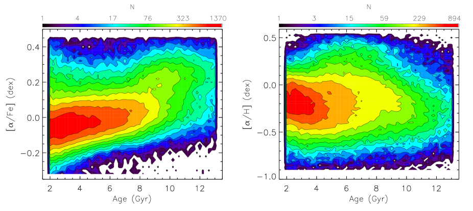
Fig. 21 plots the density distribution of the sample stars in the age–[$\alpha$/Fe] and age–[$\alpha$/H] planes. Here the [$\alpha$/H] is converted from [$\alpha$/Fe] and [Fe/H]. Only stars of ${\rm SNRs}>50$ and $T_{\rm eff}<7500$ K are used to ensure reliable [$\alpha$/Fe] estimates. Moreover, as has been discussed above, the current [$\alpha$/Fe] estimates for hot (young) stars are likely problematic, so that we further discard stars younger than 2 Gyr. Note that despite these measures, some young (e.g. $<4$ Gyr) stars with problematic [$\alpha$/Fe] estimates (e.g. $>0.2$ dex) still remain in the figure. The figure shows two sequences in the age–[$\alpha$/Fe] plane. Stars younger than 8 Gyr belong to a sequence of lower [$\alpha$/Fe] values, and the [$\alpha$/Fe] slowly increases with age in an approximately linear manner with a slope of $\lesssim$0.02 dex/Gyr. At the older end, the low-$\alpha$ sequence extends to an age older than 10 Gyr. There is also a sequence with higher [$\alpha$/Fe], which has an almost constant [$\alpha$/Fe] value of about 0.25($\pm$0.05) dex for stars older than 10 Gyr. At the younger end, the high-$\alpha$ sequence extends to $\sim$8 Gyr, when it connects with the low-$\alpha$ sequence, consistent with results from Fig. 20. The presence of two age–[$\alpha$/Fe] sequences either suggests the existence of two distinct phases of formation history of the Galactic disk (e.g. Haywood et al., 2013; Xiang et al., 2015a) or is a natural consequence of a continuous disk formation process (e.g. Schönrich & Binney, 2009b). Whatever processes have caused the multiple age–[$\alpha$/Fe] relations, it seems that 8–10 Gyr is a special epoch in the disk formation history.

The age–[$\alpha$/H] plane exhibits a significant lack of old ($>8$ Gyr), $\alpha$-rich ($>0.0$) stars, leading to a negative age–[$\alpha$/Fe] sequence at early time. At the younger end, it seems that the sequence extends to $\sim 6$ Gyr, when the [$\alpha$/H] reaches a maximum value of 0.3–0.4 dex. At any given age younger than 8 Gyr, the [$\alpha$/H] exhibits a wide distribution. Nevertheless, it seems that stars younger than 5 Gyr follow an overall negative age–[$\alpha$/H] sequence, rather than a flat one. This younger sequence has a median [$\alpha$/H] of about $-0.3$ dex at an age of 5 Gyr, and reaches a median [$\alpha$/H] value of $-0.2$ dex at 2 Gyr. At intermediate age range 5–8 Gyr, overlaps of the two sequences seem to have smoothed the negative age–[$\alpha$/H] trends. At the high-[$\alpha$/H] end, the contours show positive slopes, probably a natural consequence of the overlapping of the two sequences.

6.4. The age – metallicity relation

Figure 22.— Color-coded stellar number density distribution in the age–[Fe/H] plane. The densities are shown in logarithmic (base 10) scale.

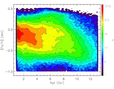
Fig. 22 plots the density distribution of the sample stars in the age–[Fe/H] plane. To ensure small uncertainties in age and [Fe/H] estimates thus to better illustrate systematic trends, only stars of ${\rm SNRs}>50$ and $T_{\rm eff}<8000$ K are shown. Stars younger than 1 Gyr are discarded for completeness (in [Fe/H]) reasons. That is, as the temperature of a MSTO star depends sensitively on both age and metallicity, a $T_{\rm eff}$ cut of 8000 K discards more metal-poor young ($<1$ Gyr) stars than metal-rich ones, thus leads to undesired trends in the age range 0–1 Gyr. The figure shows a wide range of [Fe/H] at all ages younger than 8 Gyr. At the older end ($>8$ Gyr), there is an obvious lack of metal-rich stars, yielding a relatively tight age–[Fe/H] correlation. The patterns are in good agreement with previous findings for stars in the solar-neighbourhood (e.g. Haywood et al., 2013; Bergemann et al., 2014). The relatively tight age–[Fe/H] correlation for old disk stars implies that at any given time, the interstellar medium forming the stars was relatively well-mixed. On the other hand, the broad range of [Fe/H] values for young disk stars at a given age suggests a more complicated chemical enrichment history. As the sample stars cover a large volume, one possible cause of the broad [Fe/H] distribution is the existence of both radial and vertical [Fe/H] gradients for mono-age stellar populations (Xiang et al., 2015b). However, it is also found that even in a limited volume, for instance, the solar neighborhood, the age–[Fe/H] relation for young ($<8$ Gyr) stars exhibits still a broad distribution. The inevitable presence of mixing of stars born at different positions (thus with different values of [Fe/H]) caused by stellar radial migration (e.g. Sellwood & Binney, 2002; Roškar et al., 2008; Schönrich & Binney, 2009a; Loebman et al., 2011) has certainly played a role for such [Fe/H] broadening. Whereas for very young (e.g. $\sim 1$ Gyr) stars, the broad [Fe/H] distribution is probably largely caused by sustained star formation process via accreting metal-poor gas from outside the disc, as the timescale is too short for radial migration to make a great impact.

In addition to the above qualitative patterns in agreement with the previous findings, the current large sample also reveals several interesting features. Firstly, rather than a ‘flat’ age–[Fe/H] relation, as suggested by the previous studies (e.g. Bergemann et al., 2014), young ($<5$ Gyr) disk stars seems to exhibit a negative overall trend of [Fe/H] with age, similar to that found for [$\alpha$/H]. Few studies exist on such a possible negative age–[Fe/H] trend for the young disk stars due to the limited size of stellar sample available previously. A further, more careful analysis shows that the slopes of the age–[Fe/H] relations of young stars vary with Galactocentric radius. In the outer disk, the negative age–[Fe/H] relation becomes steeper. The observed age–[Fe/H] relation of the Galactic disk is thus, similar to the age–[$\alpha$/H] relation, composed of at least two negative sequences, one for old ($\gtrsim 8$ Gyr) stars and another for young ($\lesssim$5 Gyr) stars. At the intermediate age range 5–8 Gyr, mixing of stars that follow the two separate sequences makes the trend less distinct. This two distinct sequences of age–[Fe/H] relation, if confirmed, may provide important constrains on the chemical enrichment history of the Galactic disk – it is possible that they result from two different global chemical enrichment processes of the Galactic disk. Interestingly, utilizing about 20,000 subgiant stars selected from the LAMOST DR2, Liu et al. (2015) find evidence of a ‘narrow stripe’ of stars alongside with the ‘main stripe’ stars in the age–[Fe/H] plane. They interpret those ‘narrow stripe’ stars as migrators. However, we note that their sample is less complete than ours in the age–[Fe/H] plane as their sample lacks both metal-rich and metal-poor young ($<4$ Gyr) stars (see their Fig. 7). Secondly, there is a considerable fraction of intermediate-aged (5–8 Gyr) stars of ${\rm[Fe/H]}>0.3$ dex. As a result, the density contours at the metal-rich end show positive slopes. One possible origin of these positive trends is that those metal-rich stars are migrators from the inner disk – the older the stars the further from the inside as they have longer time to reach their current positions (Loebman et al., 2011). Alternatively, a natural explanation of those positive trends is the mixing of stars from the two sequences of age–[Fe/H] relations – the intermediate-aged stars of ${\rm[Fe/H]}>0.3$ dex belong to the older sequence, whereas the young, metal-rich stars are mainly composed of stars following the younger sequence. In addition, there are a considerable number of young ($<4$ Gyr) metal-poor stars in our sample, some of them can be as metal-poor as ($\lesssim-0.6$ dex) the oldest ($>10$ Gyr) ones. The origin of those young yet metal-poor stars, as well as that for the young [$\alpha$/H]-poor stars in Fig. 21, needs to be further studied. Finally, we note that the distribution also shows a number of substructures/over-densities whose genuineness and origins remain to be further studied.

6.5. Distribution of stellar ages in the $R$ – $Z$ plane

Figure 23.— Color-coded distributions of the median age for stars in different spatial bins of the $R-Z$ plane. The adopted bin size is 0.4 kpc in the $R$ direction and 0.2 kpc in the $Z$ direction. The upper panel shows results of the whole sample stars, while the lower panel is for sample stars of $T_{\rm eff}<7000$ K.

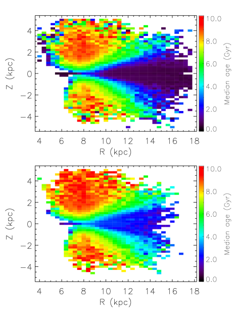
Fig. 23 plots the median age of stars at different positions across the $R$–$Z$ plane of the Galactic disk. Here $R$ is the projected Galactocentric distance in the disk mid-plane, and $Z$ the height above the disk mid-plane. The top panel presents results from all of the sample stars. Generally, the data exhibit negative age gradients in the radial and positive age gradients in the vertical direction. At small heights, the outer disk of $R\gtrsim 9$ kpc is dominated by young ($\lesssim$2 Gyr) stars, which reach larger heights above the disk plane at the farther disk, which exhibits a strong flare in median stellar age. The inner disk ($R\lesssim 9$ kpc) exhibits a positive vertical age gradient for $|Z|\lesssim 1$ kpc, while at larger heights above the disk plane, old ($\gtrsim$10 Gyr) stars dominate the population with no significant vertical gradients. However, for many bins near the boundary of the $R-Z$ plane covered by the sample stars, the stellar populations are dominated by unexpected young to intermediate-aged stars. At large height, e.g. $Z>2$ kpc, those unexpected features are likely caused by blue stragglers whose ages have been artificially underestimated, as will be discussed in §7. Those stars are usually hot and bright thus can be detected at large distances. To reduce the contaminations of blue stragglers, in the bottom panel of Fig. 23, we present the age distribution after excluding stars of $T_{\rm eff}>7000$ K. The result shows much more clean patterns, and the unexpected young populations at large heights in the inner disk now largely disappear. On the other hand, since intrinsically young stars are also discarded by the temperature cut, the outer disk exhibits systematically older ages compared to those shown in the top panel. Nevertheless, the overall structures and patterns remain unaffected.

A radial age gradient of the geometrically thick disk was also presented by Martig et al. (2016b) using giants from the APOGEE survey. A flaring young stellar disk in the outer part has been observed previously via star counts (e.g. Derriere & Robin, 2001; López-Corredoira et al., 2002; López-Corredoira & Molgó, 2014) and well reproduced by simulations (e.g. Narayan & Jog, 2002; Rahimi, Carrell & Kawata, 2014; Minchev et al., 2015) as a suggested consequence of weaker restoring force at the outer Galactocentric radii. Nevertheless, Fig. 23 demonstrates the first explicit picture of disk flare in stellar age, which will provide further constrains on disk flare models.

Note however that our results are no doubt affected by some selection effects since the sample is a magnitude limited one. Younger stars tend to be brighter thus probe larger volume than older, fainter stars. The unexpected young stellar ages near the boundary of the $R$-$Z$ plane at small heights of the inner disk are likely due to such selection effects. Age distribution in the outer disk is probably also suffering severe biases due to selection effects. A detailed and quantitative study of the selection effects of our sample stars is beyond the scope of this paper and will be presented elsewhere.

7. Unresolved binaries and blue stragglers

Figure 24.— $Upper$: Distributions of M67 member stars from Geller, Latham & Mathieu (2015) that have LAMOST observations in the ($B-V$, $V$) color-magnitude diagram (left) and the $T_{\rm eff}$ – ${\rm M}_{V}$ diagram (right). Single stars and binaries are shown by empty and filled circles, respectively. Crosses in red represent blue stragglers. The isochrones are for ages 3.5, 4.0 and 4.5 Gyr, respectively, with [Fe/H] = 0 and [$\alpha$/Fe]=0 dex. A distance modulus of 9.7 mag and a color excess $E(B-V)$ of 0.03 mag are adopted to place the isochrones in the ($B-V$, $V$) diagram. The dashed lines in the $T_{\rm eff}$–${\rm M}_{V}$ diagram denote the MSTO-SG star selection criteria for solar metallicity. $Lower$: Distributions of ages (left) and distance moduli (right) for single (black) and binary (red) members. The mean and standard deviation of the age and modulus for both single and binary members are marked in the plots.

About 40 per cent of the Galactic field stars are found in binary systems (e.g. Gao et al., 2014; Yuan et al., 2015a). The distance modulus of an unresolved binary is usually underestimated if treated as a single star, and the amount of underestimation depends on the mass ratio of the binary components, reaching a maximum of 0.75 mag in case of equal mass. This may introduce potential bias to the MSTO-SG sample. However, because binaries of high mass ratios contribute only a small fraction of the whole binary population (e.g. Duchêne & Kraus, 2013), we expect that the fraction of stars whose distances have been significantly overestimated is small in our sample. Stellar parameters of a binary could also be wrongly estimated by the current stellar parameter pipelines. Fortunately, exercises show that $T_{\rm eff}$, ${\rm M}_{V}$ and [Fe/H] derived with LSP3 from a binary spectrum are only marginally different to those derived from the spectrum of the main component star, with typical differences of only a few tens Kelvin in $T_{\rm eff}$, $<0.1$ dex in [Fe/H] and $0.1$ mag in ${\rm M}_{V}$. This is consistent with the finding of Schlesinger et al. (2010), who have analyzed the effects of binaries on stellar parameter determinations with the SDSS/SEGUE spectra.

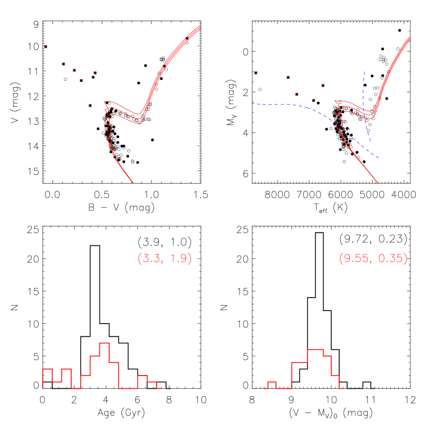
As an examination, the top right panel of Fig. 24 plots distributions of single and binary member stars of M67 from Geller, Latham & Mathieu (2015) in the $T_{\rm eff}$ – ${\rm M}_{V}$ diagram, with $T_{\rm eff}$ and M_V derived from LAMOST spectra with LSP3. The single and binary member stars of Geller, Latham & Mathieu (2015) are classified using precise radial velocity measurements. There are 142 unique single stars and 58 unique binaries that have LAMOST spectra with SNRs higher than 20. Fig. 24 shows that most of the binaries follow the same locus with single stars in both the color-magnitude and $T_{\rm eff}$–${\rm M}_{V}$ diagrams. Among those members, 62 single and 34 binary stars pass our selection criteria of MSTO-SG stars. Most single and binary MSTO-SG stars have similar age distributions, with a mean age of $\sim$4.0 Gyr and a standard deviation of $\sim$1.0 Gyr. There are a few outliers in the age distribution of binary members. Among them, the younger ones are blue stragglers, while the older ones are likely contaminations of main sequence binary stars with large parameter uncertainties. The distributions of distance moduli of the single and binary populations exhibit some discrepancies, in the sense that binaries yield a mean modulus 0.17 mag smaller than single stars due to their brighter apparent magnitudes. The difference corresponds to a $\sim$10 per cent underestimation of their distances.

Blue straggler stars (BSS) are generally believed to be products of coalescence or mass exchange in binary evolution (e.g. Chen & Han, 2008a, b), and as a result, they are more luminous and bluer than MSTO stars of the same age. The ages of those stars may have been artificially underestimated with our current method. An accurate determination of the fraction of BSS with respect to the whole stellar population has not been carried out, although we expect this number to be considerable considering that there are large number of such stars in our sample. As for M67 shown in Fig. 24, 6–8 out of the 98 MSTO-SG stars ($\sim$7 per cent) are BSS according to the identification of Geller, Latham & Mathieu (2015). For our MSTO-SG star sample, exercises show that at $|Z|>1.5$ kpc, about 4 per cent stars have age estimates younger than 2 Gyr. Since young stars are not expected to occur at such a large height away from the disk midplane, they are likely BSS stars whose ages have been artificially underestimated. Contamination rate of BSS to truly young stars having comparable ages as estimated for the BSS should be even higher and needs to be further studied. As a rough estimate, we can simply assume that for sample stars of 2–12 Gyr, 4 per cent are actually BSS whose ages have been wrongly underestimated to be younger than $2$ Gyr. If we further assume that the star formation rate of the Milky Way disk is flat, then the total contamination of BSS to the young sample stars ($<2$ Gyr) is about 20 per cent.

8. Summary

A sample of 0.93 million disk MSTO and subgiant stars are defined using the value-added catalog of the LAMOST Galactic Spectroscopic Surveys. Stellar masses and ages of the sample stars are estimated with a Bayesian algorithm based on stellar isochrones. Uncertainties of the resultant parameters depend on the SNR, and have a typical (median) value of $0.08$ ${\rm M}_{\odot}$ in mass and 34 per cent in age, and half of the sample stars older than 2 Gyr have age uncertainties of only 20–30 per cent. Robustness of the results are validated via examinations with extensive datasets, including a mock dataset, the LAMOST-TGAS common stars, LAMOST-$Kepler$ common stars that have asteroseismic parameters, member stars of open clusters as well as duplicate observations of the sample stars. In addition to the random errors, there is probably also a systematic uncertainty of about 1–2 Gyr in the age estimates as a consequence of inadequate model assumptions of stellar isochrones as well as inadequacy in the analysis method. For the young stellar populations, contaminations from blue straggler stars are non-negligible.

Interesting patterns are seen in the distribution of median age across the [Fe/H]–[$\alpha$/Fe] plane. As expected, metal-poor, $\alpha$-enhanced stars are generally older than metal-rich, $\alpha$-poor stars. The most metal-poor (${\rm[Fe/H]}<-0.5$ dex) and $\alpha$-enhanced (${\rm[\alpha/Fe]}>0.2$ dex) stars have median ages older than 10 Gyr. Stars of intermediate-to-old ages (5–8 Gyr) exhibit a contiguous distribution across the whole metallicity range from $-1.0$ to 0.5 dex and have a clear demarcation from younger, more $\alpha$-poor ([$\alpha$/Fe]$\lesssim 0.0$ dex) stars. The latter shows an age gradient with [Fe/H]. Stellar density distribution in the [Fe/H]–[$\alpha$/Fe] plane exhibits both thin and thick disk sequences for stars of 8–10 Gyr, while only the thin (thick) disk sequence is present for younger (older) stars, implying that the thin disk became prominent 8–10 Gyr ago, while the thick disk was formed at an earlier epoch and was almost quenched 8 Gyr ago.

Good correlations between age and [$\alpha$/Fe] or [$\alpha$/H] (and [Fe/H]) are found. There are two correlation sequences in the age–[$\alpha$/Fe] plane. The lower-$\alpha$ sequence contains stars with ages ranging from younger than 1 to older than 10 Gyr, and the [$\alpha$/Fe] values slowly increase with age in an approximately linear manner with a slope of $\lesssim$0.02 dex/Gyr. The higher-$\alpha$ sequence is composed of relatively old ($>8$ Gyr) stars, and the [$\alpha$/Fe] values are almost constant ($\sim$0.25 dex) for stars older than 10 Gyr, and then decrease with age in the range 8–10 Gyr. The sample stars exhibit also two sequences in the age–[Fe/H] and age–[$\alpha$/H] planes. There is a lack of metal-rich stars older than 8 Gyr, which forms a negative age–[Fe/H] sequence. This older sequence seems to reach $\sim$5–6 Gyr at the younger end, with [Fe/H] increasing from $\sim-0.6$ dex at 12 Gyr to $\sim$0.3 dex at 6 Gyr. Instead of a ‘flat’ distribution, the huge sample reveals also a significant negative age–[Fe/H] sequence for stars younger than $\sim$5 Gyr. At intermediate ages of about 5–8 Gyr, mixing of stars from the two sequences makes the negative age–[Fe/H] correlations less obvious. Similar trends are seen in the age–[$\alpha$/H] plane. Moreover, at the lower-[$\alpha$/H] side, the younger sequence seems to have [$\alpha$/H] values lower than those of the older sequence.

The sample stars exhibit interesting age structures across the disk of $4<R<18$ kpc. The median stellar age increases with $Z$ and decreases with $R$, yielding a positive age gradient in the vertical and a negative gradient in the radial direction of the disk. At the outer disk of $R\gtrsim 9$ kpc, the stellar age shows a strong flaring structure, which is expected to provide further constrains on disk flare models.

Acknowledgments It is a pleasure to thank the anonymous referee for valuable comments and suggestions. This work is supported by Joint Funds of the National Natural Science Foundation of China (Grant No. U1531244) and National Key Basic Research Program of China 2014CB845700. Z.-Y. Huo and M.-S. Xiang acknowledge supports from the National Natural Science Foundation of China (NSFC, Grant No. 11403038). H.-B. Yuan acknowledges supports from NSFC grant No. 11443006, No. 11603002 and Beijing Normal University grant No. 310232102. The LAMOST FELLOWSHIP is supported by Special Funding for Advanced Users, budgeted and administrated by Center for Astronomical Mega-Science, Chinese Academy of Sciences (CAMS).

Guoshoujing Telescope (the Large Sky Area Multi-Object Fiber Spectroscopic Telescope LAMOST) is a National Major Scientific Project built by the Chinese Academy of Sciences. Funding for the project has been provided by the National Development and Reform Commission. LAMOST is operated and managed by the National Astronomical Observatories, Chinese Academy of Sciences.

Appendix A

Table 2Trajectories of MSTO in the $T_{\rm eff}$ – ${\rm M}_{V}$ plane, ${\rm M}_{V}^{\rm TO}$ = $a_{0}$ + $a_{1}\times$$T_{\rm eff}$ + $a_{2}\times$$T_{\rm eff}^{2}$ + $a_{3}\times$$T_{\rm eff}^{3}$ + $a_{4}\times$$T_{\rm eff}^{4}$, as well as the adopted minimum temperature of MSTO of isochrones, $T_{\rm eff}^{\rm MINISO}$.

[Fe/H]	[$\alpha$/Fe]	$a_{0}$	$a_{1}$	$a_{2}$	$a_{3}$	$a_{4}$	$T_{\rm eff}^{\rm MINISO}$ (K)
$-1.0$	0.30	32.9210	$-0.00828$	5.10153e$-07$	2.79169e$-11$	$-$2.79516e$-15$	5678
$-0.9$	0.28	24.8208	$-0.00376$	$-$4.27601e$-07$	1.13254e$-10$	$-$5.67469e$-15$	5637
$-0.8$	0.26	15.5995	0.00139	$-$1.50012e$-06$	2.11171e$-10$	$-$8.99138e$-15$	5594
$-0.7$	0.24	6.4951	0.00655	$-$2.58761e$-06$	3.11700e$-10$	$-$1.24379e$-14$	5546
$-0.6$	0.22	$-3.6820$	0.01233	$-$3.80997e$-06$	4.25071e$-10$	$-$1.63391e$-14$	5497
$-0.5$	0.20	$-13.6972$	0.01810	$-$5.04614e$-06$	5.41152e$-10$	$-$2.03809e$-14$	5450
$-0.4$	0.16	$-24.1542$	0.02418	$-$6.35876e$-06$	6.65373e$-10$	$-$2.47385e$-14$	5416
$-0.3$	0.12	$-35.6453$	0.03088	$-$7.81131e$-06$	8.03316e$-10$	$-$2.95945e$-14$	5377
$-0.2$	0.08	$-46.9116$	0.03755	$-$9.27544e$-06$	9.44030e$-10$	$-$3.46030e$-14$	5335
$-0.1$	0.04	$-59.0560$	0.04477	$-$1.08696e$-05$	1.09792e$-09$	$-$4.01032e$-14$	5268
0.0	0.00	$-71.1208$	0.05205	$-$1.24941e$-05$	1.25640e$-09$	$-$4.58219e$-14$	5253
0.1	0.00	$-83.8769$	0.05979	$-$1.42343e$-05$	1.42708e$-09$	$-$5.20100e$-14$	5179
0.2	0.00	$-96.9268$	0.06781	$-$1.60510e$-05$	1.60669e$-09$	$-$5.85678e$-14$	5175
0.3	0.00	$-110.4560$	0.07619	$-$1.79643e$-05$	1.79699e$-09$	$-$6.55526e$-14$	5130
0.4	0.00	$-124.7290$	0.08510	$-$2.00142e$-05$	2.00203e$-09$	$-$7.31135e$-14$	5096
0.5	0.00	$-139.8100$	0.09455	$-$2.21929e$-05$	2.22051e$-09$	$-$8.11890e$-14$	5287

Table 3Trajectories of base RGB in the $T_{\rm eff}$ – ${\rm M}_{V}$ plane, $T_{\rm eff}^{\rm bRGB}$ = $b_{0}$ + $b_{1}\times{\rm M}_{V}$ + $b_{2}\times{\rm M}_{V}^{2}$ + $a_{3}\times{\rm M}_{V}^{3}$.

[Fe/H]	[$\alpha$/Fe]	$b_{0}$	$b_{1}$	$b_{2}$	$b_{3}$
$-1.0$	0.30	5156.16	107.612	$-5.41575$	$-6.10802$
$-0.9$	0.28	5126.67	111.224	$-7.62809$	$-5.80089$
$-0.8$	0.26	5096.75	112.755	$-8.75758$	$-5.62243$
$-0.7$	0.24	5068.06	111.355	$-8.75119$	$-5.55727$
$-0.6$	0.22	5039.51	109.027	$-8.36525$	$-5.52200$
$-0.5$	0.20	5010.91	106.143	$-7.72652$	$-5.49936$
$-0.4$	0.16	4982.45	102.590	$-6.79953$	$-5.48756$
$-0.3$	0.12	4954.27	98.2728	$-5.55812$	$-5.48322$
$-0.2$	0.08	4925.72	94.5977	$-4.56288$	$-5.42086$
$-0.1$	0.04	4896.64	92.3138	$-4.14167$	$-5.25891$
0.0	0.00	4868.28	89.1947	$-3.41834$	$-5.08543$
0.1	0.00	4840.10	86.5965	$-2.94804$	$-4.83513$
0.2	0.00	4812.81	83.2880	$-2.25062$	$-4.55325$
0.3	0.00	4786.01	80.3599	$-1.76849$	$-4.18724$
0.4	0.00	4760.20	77.1021	$-1.23815$	$-3.75894$
0.5	0.00	4735.49	73.5323	$-0.679470$	$-3.26016$

References

- Balaguer-Núñez, Galadí-Enríquez & Jordi (2007) Balaguer-Núñez L., Galadí-Enríquez D., Jordi C., 2007, A&A, 470, 585
- Barnes et al. (2016) Barnes S. A., Weingrill J., Fritzewski D., Strassmeier K. G., Platais I., 2016, ApJ, 823, 16
- Bensby, Feltzing & Lundström (2003) Bensby T., Feltzing S., Lundström I., 2003, A&A, 410, 527
- Bergemann et al. (2014) Bergemann M. et al., 2014, A&A, 565, A89
- Bessell (1979) Bessell M. S., 1979, PASP, 91, 589
- Bessell (2005) Bessell M. S., 2005, ARA&A, 43, 293
- Bessell & Brett (1988) Bessell M. S., Brett J. M., 1988, PASP, 100, 1134
- Bressan et al. (2012) Bressan A., Marigo P., Girardi L., Salasnich B., Dal Cero C., Rubele S., Nanni A., 2012, MNRAS, 427, 127
- Buser (1978) Buser R., 1978, A&A, 62, 411
- Carraro et al. (1994) Carraro G., Chiosi C., Bressan A., Bertelli G., 1994, A&AS, 103
- Casagrande et al. (2010) Casagrande L., Ramírez I., Meléndez J., Bessell M., Asplund M., 2010, A&A, 512, A54
- Chabrier (2003) Chabrier G., 2003, PASP, 115, 763
- Chaplin et al. (2014) Chaplin W. J. et al., 2014, ApJS, 210, 1
- Chen & Han (2008a) Chen X., Han Z., 2008a, MNRAS, 384, 1263
- Chen & Han (2008b) Chen X., Han Z., 2008b, MNRAS, 387, 1416
- Creevey et al. (2013) Creevey O. L. et al., 2013, MNRAS, 431, 2419
- De Cat et al. (2015) De Cat P. et al., 2015, ApJS, 220, 19
- Demarque, Green & Guenther (1992) Demarque P., Green E. M., Guenther D. B., 1992, AJ, 103, 151
- Demarque, Sarajedini & Guo (1994) Demarque P., Sarajedini A., Guo X.-J., 1994, ApJ, 426, 165
- Demarque et al. (2004) Demarque P., Woo J.-H., Kim Y.-C., Yi S. K., 2004, ApJS, 155, 667
- Deng et al. (2012) Deng L.-C. et al., 2012, Research in Astronomy and Astrophysics, 12, 735
- Derriere & Robin (2001) Derriere S., Robin A. C., 2001, in Astronomical Society of the Pacific Conference Series, Vol. 232, The New Era of Wide Field Astronomy, Clowes R., Adamson A., Bromage G., eds., p. 229
- Dinescu et al. (1995) Dinescu D. I., Demarque P., Guenther D. B., Pinsonneault M. H., 1995, AJ, 109, 2090
- D’Orazi et al. (2006) D’Orazi V., Bragaglia A., Tosi M., Di Fabrizio L., Held E. V., 2006, MNRAS, 368, 471
- Dotter et al. (2008) Dotter A., Chaboyer B., Jevremović D., Kostov V., Baron E., Ferguson J. W., 2008, ApJS, 178, 89
- Duchêne & Kraus (2013) Duchêne G., Kraus A., 2013, ARA&A, 51, 269
- Edvardsson et al. (1993) Edvardsson B., Andersen J., Gustafsson B., Lambert D. L., Nissen P. E., Tomkin J., 1993, A&A, 275, 101
- Fan et al. (1996) Fan X. et al., 1996, AJ, 112, 628
- Fuhrmann (1998) Fuhrmann K., 1998, A&A, 338, 161
- Gai et al. (2011) Gai N., Basu S., Chaplin W. J., Elsworth Y., 2011, ApJ, 730, 63
- Gaia Collaboration et al. (2016) Gaia Collaboration et al., 2016, A&A, 595, A2
- Gao et al. (2014) Gao S., Liu C., Zhang X., Justham S., Deng L., Yang M., 2014, ApJ, 788, L37
- Geller, Latham & Mathieu (2015) Geller A. M., Latham D. W., Mathieu R. D., 2015, AJ, 150, 97
- Hayden et al. (2015) Hayden M. R. et al., 2015, ApJ, 808, 132
- Haywood et al. (2013) Haywood M., Di Matteo P., Lehnert M. D., Katz D., Gómez A., 2013, A&A, 560, A109
- Hekker et al. (2013) Hekker S., Elsworth Y., Mosser B., Kallinger T., Basu S., Chaplin W. J., Stello D., 2013, A&A, 556, A59
- Hills et al. (2015) Hills S., von Hippel T., Courteau S., Geller A. M., 2015, AJ, 149, 94
- Ho et al. (2016) Ho A. Y. Q., Rix H.-W., Ness M. K., Hogg D. W., Liu C., Ting Y.-S., 2016, ArXiv e-prints
- Hou et al. (2013) Hou J. L., Zhong J., Chen L., Yu J. C., Liu C., Deng L. C., 2013, in IAU Symposium, Vol. 292, IAU Symposium, Wong T., Ott J., eds., pp. 105–105
- Huang et al. (2015) Huang Y., Liu X.-W., Yuan H.-B., Xiang M.-S., Chen B.-Q., Zhang H.-W., 2015, MNRAS, 454, 2863
- Huber et al. (2014) Huber D. et al., 2014, ApJS, 211, 2
- Jørgensen & Lindegren (2005) Jørgensen B. R., Lindegren L., 2005, A&A, 436, 127
- Kalirai et al. (2003) Kalirai J. S., Fahlman G. G., Richer H. B., Ventura P., 2003, AJ, 126, 1402
- Kaluzny & Mazur (1991) Kaluzny J., Mazur B., 1991, Acta Astron., 41, 167
- Kroupa (2001) Kroupa P., 2001, MNRAS, 322, 231
- Kroupa et al. (2013) Kroupa P., Weidner C., Pflamm-Altenburg J., Thies I., Dabringhausen J., Marks M., Maschberger T., 2013, The Stellar and Sub-Stellar Initial Mass Function of Simple and Composite Populations, Oswalt T. D., Gilmore G., eds., p. 115
- Lee et al. (2011) Lee Y. S. et al., 2011, ApJ, 738, 187
- Lejeune, Cuisinier & Buser (1998) Lejeune T., Cuisinier F., Buser R., 1998, A&AS, 130, 65
- Li et al. (2016) Li J. et al., 2016, Research in Astronomy and Astrophysics, 16, 110
- Lindegren et al. (2016) Lindegren L. et al., 2016, A&A, 595, A4
- Liu et al. (2015) Liu C. et al., 2015, ArXiv e-prints
- Liu et al. (2014) Liu X.-W. et al., 2014, in IAU Symposium, Vol. 298, IAU Symposium, Feltzing S., Zhao G., Walton N. A., Whitelock P., eds., pp. 310–321
- Loebman et al. (2011) Loebman S. R., Roškar R., Debattista V. P., Ivezić Ž., Quinn T. R., Wadsley J., 2011, ApJ, 737, 8
- López-Corredoira et al. (2002) López-Corredoira M., Cabrera-Lavers A., Garzón F., Hammersley P. L., 2002, A&A, 394, 883
- López-Corredoira & Molgó (2014) López-Corredoira M., Molgó J., 2014, A&A, 567, A106
- Luo et al. (2012) Luo A.-L. et al., 2012, Research in Astronomy and Astrophysics, 12, 1243
- Luo et al. (2015) Luo A.-L. et al., 2015, Research in Astronomy and Astrophysics, 15, 1095
- Martig et al. (2016a) Martig M. et al., 2016a, MNRAS, 456, 3655
- Martig et al. (2016b) Martig M., Minchev I., Ness M., Fouesneau M., Rix H.-W., 2016b, ApJ, 831, 139
- Meibom, Mathieu & Stassun (2009) Meibom S., Mathieu R. D., Stassun K. G., 2009, ApJ, 695, 679
- Michalik, Lindegren & Hobbs (2015) Michalik D., Lindegren L., Hobbs D., 2015, A&A, 574, A115
- Minchev et al. (2015) Minchev I., Martig M., Streich D., Scannapieco C., de Jong R. S., Steinmetz M., 2015, ApJ, 804, L9
- Narayan & Jog (2002) Narayan C. A., Jog C. J., 2002, A&A, 390, L35
- Nordström et al. (2004) Nordström B. et al., 2004, A&A, 418, 989
- Planck Collaboration et al. (2016) Planck Collaboration et al., 2016, A&A, 594, A13
- Rahimi, Carrell & Kawata (2014) Rahimi A., Carrell K., Kawata D., 2014, Research in Astronomy and Astrophysics, 14, 1406
- Ren et al. (2016) Ren J.-J. et al., 2016, Research in Astronomy and Astrophysics, 16, 045
- Richer et al. (1998) Richer H. B., Fahlman G. G., Rosvick J., Ibata R., 1998, ApJ, 504, L91
- Richtler & Sagar (2001) Richtler T., Sagar R., 2001, Bulletin of the Astronomical Society of India, 29, 53
- Roškar et al. (2008) Roškar R., Debattista V. P., Quinn T. R., Stinson G. S., Wadsley J., 2008, ApJ, 684, L79
- Salaris, Weiss & Percival (2004) Salaris M., Weiss A., Percival S. M., 2004, A&A, 414, 163
- Salpeter (1955) Salpeter E. E., 1955, ApJ, 121, 161
- Sánchez-Blázquez et al. (2006) Sánchez-Blázquez P. et al., 2006, MNRAS, 371, 703
- Santos, Israelian & Mayor (2004) Santos N. C., Israelian G., Mayor M., 2004, A&A, 415, 1153
- Sarajedini, Dotter & Kirkpatrick (2009) Sarajedini A., Dotter A., Kirkpatrick A., 2009, ApJ, 698, 1872
- Schiavon, Caldwell & Rose (2004) Schiavon R. P., Caldwell N., Rose J. A., 2004, AJ, 127, 1513
- Schlegel, Finkbeiner & Davis (1998) Schlegel D. J., Finkbeiner D. P., Davis M., 1998, ApJ, 500, 525
- Schlesinger et al. (2010) Schlesinger K. J., Johnson J. A., Lee Y. S., Masseron T., Yanny B., Rockosi C. M., Gaudi B. S., Beers T. C., 2010, ApJ, 719, 996
- Schönrich & Binney (2009a) Schönrich R., Binney J., 2009a, MNRAS, 396, 203
- Schönrich & Binney (2009b) Schönrich R., Binney J., 2009b, MNRAS, 399, 1145
- Sellwood & Binney (2002) Sellwood J. A., Binney J. J., 2002, MNRAS, 336, 785
- Soderblom (2010) Soderblom D. R., 2010, ARA&A, 48, 581
- Takeda et al. (2007) Takeda G., Ford E. B., Sills A., Rasio F. A., Fischer D. A., Valenti J. A., 2007, ApJS, 168, 297
- Tosi, Bragaglia & Cignoni (2007) Tosi M., Bragaglia A., Cignoni M., 2007, MNRAS, 378, 730
- Twarog, Anthony-Twarog & Bricker (1999) Twarog B. A., Anthony-Twarog B. J., Bricker A. R., 1999, AJ, 117, 1816
- Valenti & Fischer (2005) Valenti J. A., Fischer D. A., 2005, ApJS, 159, 141
- VandenBerg & Stetson (2004) VandenBerg D. A., Stetson P. B., 2004, PASP, 116, 997
- von Hippel et al. (2002) von Hippel T., Steinhauer A., Sarajedini A., Deliyannis C. P., 2002, AJ, 124, 1555
- Wu et al. (2014) Wu Y., Du B., Luo A., Zhao Y., Yuan H., 2014, in IAU Symposium, Vol. 306, Statistical Challenges in 21st Century Cosmology, Heavens A., Starck J.-L., Krone-Martins A., eds., pp. 340–342
- Wu et al. (2017) Wu Y.-Q. et al., 2017, Research in Astronomy and Astrophysics, 17, 5
- Xiang et al. (2017a) Xiang M.-S. et al., 2017a, MNRAS, 464, 3657
- Xiang et al. (2015a) Xiang M. S. et al., 2015a, MNRAS, 448, 822
- Xiang et al. (2015b) Xiang M.-S. et al., 2015b, Research in Astronomy and Astrophysics, 15, 1209
- Xiang et al. (2017b) Xiang M.-S. et al., 2017b, MNRAS, 467, 1890
- Xiang et al. (2015c) Xiang M. S. et al., 2015c, MNRAS, 448, 90
- Yuan et al. (2015a) Yuan H., Liu X., Xiang M., Huang Y., Chen B., Wu Y., Hou Y., Zhang Y., 2015a, ApJ, 799, 135
- Yuan et al. (2015b) Yuan H.-B. et al., 2015b, MNRAS, 448, 855
- Yuan, Liu & Xiang (2013) Yuan H. B., Liu X. W., Xiang M. S., 2013, MNRAS, 430, 2188
- Zacharias et al. (2013) Zacharias N., Finch C. T., Girard T. M., Henden A., Bartlett J. L., Monet D. G., Zacharias M. I., 2013, AJ, 145, 44
- Zhao et al. (2012) Zhao G., Zhao Y.-H., Chu Y.-Q., Jing Y.-P., Deng L.-C., 2012, Research in Astronomy and Astrophysics, 12, 723