Acceleration and Averaging
In Stochastic Mirror Descent Dynamics

Walid Krichene Research and Machine Intelligence, Google Inc. walidk@google.com    Peter Bartlett Department of Statistics and Computer Science division, University of California at Berkeley, and Queensland University of Technology. bartlett@cs.berkeley.edu
Abstract

We formulate and study a general family of (continuous-time) stochastic dynamics for accelerated first-order minimization of smooth convex functions.

Building on an averaging formulation of accelerated mirror descent, we propose a stochastic variant in which the gradient is contaminated by noise, and study the resulting stochastic differential equation. We prove a bound on the rate of change of an energy function associated with the problem, then use it to derive estimates of convergence rates of the function values, (a.s. and in expectation) both for persistent and asymptotically vanishing noise. We discuss the interaction between the parameters of the dynamics (learning rate and averaging weights) and the covariation of the noise process, and show, in particular, how the asymptotic rate of covariation affects the choice of parameters and, ultimately, the convergence rate.

1 Introduction

We consider the constrained convex minimization problem

minxβˆˆπ’³β‘f​(x),subscriptπ‘₯𝒳𝑓π‘₯\min_{x\in\mathcal{X}}f(x),

where 𝒳𝒳\mathcal{X} is a closed, convex, subset of E=ℝn𝐸superscriptℝ𝑛E=\mathbb{R}^{n}, and f𝑓f is a proper closed convex function, assumed to be differentiable with Lipschitz gradient, and we will denote 𝒳⋆superscript𝒳⋆\mathcal{X}^{\star} the set of minimizers of this problem, assumed to be non-empty. First-order optimization methods play an important role in minimizing such functions, in particular in large-scale machine learning applications, in which the dimensionality (number of features) and size (number of samples) in typical datasets makes higher-order methods intractable. Many such algorithms can be viewed as a discretization of a continuous-time dynamics. The simplest example is gradient descent, which can be viewed as the discretization of the gradient flow dynamics x˙​(t)=βˆ’βˆ‡f​(x​(t))Λ™π‘₯π‘‘βˆ‡π‘“π‘₯𝑑\dot{x}(t)=-\nabla f(x(t)), where x˙​(t)Λ™π‘₯𝑑\dot{x}(t) denotes the time derivative of a C1superscript𝐢1C^{1} trajectory x​(t)π‘₯𝑑x(t). An important generalization of gradient descent, which elegantly handles the constraint set 𝒳𝒳\mathcal{X}, was developed byΒ Nemirovsky and Yudin (1983), and termed mirror descent: it couples a dual variable z​(t)𝑧𝑑z(t) accumulating gradients, and its β€œmirror” primal variableΒ x​(t)π‘₯𝑑x(t). More specifically, the dynamics are given by

MD⁑{z˙​(t)=βˆ’βˆ‡f​(x​(t))x​(t)=βˆ‡Οˆβˆ—β€‹(z​(t)),MDcasesΛ™π‘§π‘‘βˆ‡π‘“π‘₯𝑑otherwiseπ‘₯π‘‘βˆ‡superscriptπœ“π‘§π‘‘otherwise\operatorname{MD}\begin{cases}\dot{z}(t)=-\nabla f(x(t))\\ x(t)=\nabla\psi^{*}(z(t)),\end{cases} (1)

where βˆ‡Οˆβˆ—:Eβˆ—β†’π’³:βˆ‡superscriptπœ“β†’superscript𝐸𝒳\nabla\psi^{*}:E^{*}\to\mathcal{X} is a Lipschitz function defined on the entire dual space Eβˆ—superscript𝐸E^{*}, with values in the feasible set 𝒳𝒳\mathcal{X}; it is often referred to as a mirror map, and we will recall its definition and properties in SectionΒ 2. Mirror descent can be viewed as a generalization of projected gradient descent, where the Euclidean projection is replaced by the mirror map βˆ‡Οˆβˆ—βˆ‡superscriptπœ“\nabla\psi^{*}Β (Beck and Teboulle, 2003). This makes it possible to adapt the choice of the mirror map to the particular geometry of the problem, leading to closed-form solutions of the projection, or to better dependence on the dimension n𝑛n, seeΒ (Ben-Tal and Nemirovski, 2001), (Ben-Tal etΒ al., 2001).

Continuous-time dynamics

Although optimization methods are inherently discrete, the continuous-time point of view can help in their design and analysis, since it can leverage the rich literature on dynamical systems, control theory, and mechanics, seeΒ (Helmke and Moore, 1994), (Bloch, 1994), and the references therein. Continuous-time models are also commonly used in financial applications, such as option pricingΒ (Black and Scholes, 1973), even though the actions are taken in discrete time. In convex optimization, beyond simplifying the analysis, continuous-time models have also motivated new algorithms and heuristics: mirror descent is one such example, since it was originally motivated in continuous-time (Chapter 3 inΒ (Nemirovsky and Yudin, 1983)). In a more recent line of work ((Su etΒ al., 2014), (Krichene etΒ al., 2015), (Wibisono etΒ al., 2016)), Nesterov’s accelerated methodΒ (Nesterov, 1983) was shown to be the discretization of a second-order ordinary differential equation (ODE), which, in the unconstrained case, can be interpreted as a damped non-linear oscillatorΒ (Cabot etΒ al., 2009; Attouch etΒ al., 2015). This motivated a restarting heuristic (O’Donoghue and CandΓ¨s, 2015), which aims at further dissipating the energy of the oscillator. Krichene etΒ al. (2015) generalized this ODE to mirror descent dynamics, and gave an averaging interpretation (a connection which was previously pointed out byΒ Flammarion and Bach (2015) for quadratic functions). This averaging formulation is the starting point of this paper, in which we introduce and study a stochastic variant of accelerated mirror descent dynamics.

Stochastic dynamics and related work

The dynamics which we discussed so far (gradient descent, mirror descent, and their accelerated variants) are deterministic first-order dynamics, since they use the exact gradient βˆ‡fβˆ‡π‘“\nabla f. However, in many machine learning applications, evaluating the exact gradient βˆ‡fβˆ‡π‘“\nabla f can be prohibitively expensive, e.g. when the objective function f𝑓f involves the sum of loss functions over a training set, of the form f​(x)=1|ℐ|β€‹βˆ‘iβˆˆβ„fi​(x)+g​(x)𝑓π‘₯1ℐsubscript𝑖ℐsubscript𝑓𝑖π‘₯𝑔π‘₯f(x)=\frac{1}{|\mathcal{I}|}\sum_{i\in\mathcal{I}}f_{i}(x)+g(x), where ℐℐ\mathcal{I} indexes the training samples, and g𝑔g is a regularization function. Instead of computing the exact gradient βˆ‡f​(x)=1|ℐ|β€‹βˆ‘iβˆˆβ„βˆ‡fi​(x)+βˆ‡g​(x)βˆ‡π‘“π‘₯1ℐsubscriptπ‘–β„βˆ‡subscript𝑓𝑖π‘₯βˆ‡π‘”π‘₯\nabla f(x)=\frac{1}{|\mathcal{I}|}\sum_{i\in\mathcal{I}}\nabla f_{i}(x)+\nabla g(x), a common approach is to compute an unbiased, stochastic estimate of the gradient, given by 1|ℐ~|β€‹βˆ‘iβˆˆβ„~βˆ‡fi​(x)+βˆ‡g​(x)1~ℐsubscript𝑖~β„βˆ‡subscript𝑓𝑖π‘₯βˆ‡π‘”π‘₯\frac{1}{|\tilde{\mathcal{I}}|}\sum_{i\in\tilde{\mathcal{I}}}\nabla f_{i}(x)+\nabla g(x), where I~~𝐼\tilde{I} is a uniformly random subset of ℐℐ\mathcal{I}, indexing a random batch of samples from the training set. This approach motivates the study of stochastic dynamics for convex optimization. But despite an extensive literature on stochastic gradient and mirror descent in discrete time, e.g. (Nemirovski etΒ al., 2009), (Duchi etΒ al., 2010), (Lan, 2012), (Johnson and Zhang, 2013), (Xiao and Zhang, 2014), and many others, few results are known for stochastic mirror descent in continuous-time. To the best of our knowledge, the only published results are by Raginsky and Bouvrie (2012) and Mertikopoulos and Staudigl (2016).

In its simplest form, the stochastic gradient flow dynamics can be described by the Itô stochastic differential equation (SDE) (Øksendal, 2003)

d​X​(t)=βˆ’βˆ‡f​(X​(t))+σ​d​B​(t),π‘‘π‘‹π‘‘βˆ‡π‘“π‘‹π‘‘πœŽπ‘‘π΅π‘‘dX(t)=-\nabla f(X(t))+\sigma dB(t),

where B​(t)𝐡𝑑B(t) denotes a standard Wiener process (Brownian motion). It is well known that this dynamics admits a unique invariant measure with density proportional to the Gibbs distribution eβˆ’2​f​(x)Οƒsuperscript𝑒2𝑓π‘₯𝜎e^{-\frac{2f(x)}{\sigma}}. Such dynamics have recently played an important role in the analysis of sampling methodsΒ (Dalalyan, 2017), (Bubeck etΒ al., 2015), (Cheng and Bartlett, 2017), (Cheng etΒ al., 2017), where f𝑓f is taken to be the logarithm of a target distribution p𝑝p. The stationary distribution of the SDE has also been recently interpreted as an approximate Bayesian inferenceΒ (Mandt etΒ al., 2017), and to derive convergence rates (in expectation) for smooth, non-convex optimization where the objective is dissipativeΒ (Raginsky etΒ al., 2017).

For mirror descent dynamics, Raginsky and Bouvrie (2012) were the first to propose a stochastic variant of the mirror descent ODEΒ (1), given by the ItΓ΄ SDE:

SMD⁑{d​Z​(t)=βˆ’βˆ‡f​(X​(t))+σ​d​B​(t)X​(t)=βˆ‡Οˆβˆ—β€‹(Z​(t))SMDcasesπ‘‘π‘π‘‘βˆ‡π‘“π‘‹π‘‘πœŽπ‘‘π΅π‘‘otherwiseπ‘‹π‘‘βˆ‡superscriptπœ“π‘π‘‘otherwise\operatorname{SMD}\begin{cases}dZ(t)=-\nabla f(X(t))+\sigma dB(t)\\ X(t)=\nabla\psi^{*}(Z(t))\end{cases} (2)

where ΟƒπœŽ\sigma is a constant volatility. In particular, they argued that the function values f​(X​(t))𝑓𝑋𝑑f(X(t)) along sample trajectories do not converge to the minimum value of f𝑓f due to the persistent noise, but the optimality gap is bounded by a quantity proportional to Οƒ2superscript𝜎2\sigma^{2}. They also proposed a method to reduce the variance by simultaneously sampling multiple trajectories and linearly coupling them. Mertikopoulos and Staudigl (2016) extended the analysis in some important directions: they replaced the constant volatility ΟƒπœŽ\sigma with a general volatility matrix σ​(x,t)𝜎π‘₯𝑑\sigma(x,t) which can depend on the current point xπ‘₯x and current time t𝑑t, and studied two regimes: the vanishing noise regime given by the condition supxβˆˆπ’³Οƒβ€‹(x,t)=o​(1/log⁑t)subscriptsupremumπ‘₯π’³πœŽπ‘₯π‘‘π‘œ1𝑑\sup_{x\in\mathcal{X}}\sigma(x,t)=o(1/\sqrt{\log t}), in which case they prove almost sure convergence of solution trajectories; and the persistent noise regime, given by the condition supxβˆˆπ’³Οƒβ€‹(x,t)β‰€Οƒβˆ—subscriptsupremumπ‘₯π’³πœŽπ‘₯𝑑subscript𝜎\sup_{x\in\mathcal{X}}\sigma(x,t)\leq\sigma_{*} uniformly in t𝑑t, in which case they define a rectified variant of SMDSMD\operatorname{SMD}, obtained by replacing the second equation by X​(t)=βˆ‡Οˆβˆ—β€‹(Z​(t)/s​(t))π‘‹π‘‘βˆ‡superscriptπœ“π‘π‘‘π‘ π‘‘X(t)=\nabla\psi^{*}(Z(t)/s(t)), where 1/s​(t)1𝑠𝑑1/s(t) is a sensitivity parameter. The resulting dynamics is given by

SMDs⁑{Z˙​(t)=βˆ’βˆ‡f​(X​(t))+σ​(X​(t),t)​d​B​(t),X​(t)=βˆ‡Οˆβˆ—β€‹(Z​(t)/s​(t)).subscriptSMD𝑠casesΛ™π‘π‘‘βˆ‡π‘“π‘‹π‘‘πœŽπ‘‹π‘‘π‘‘π‘‘π΅π‘‘otherwiseπ‘‹π‘‘βˆ‡superscriptπœ“π‘π‘‘π‘ π‘‘otherwise\operatorname{SMD}_{s}\begin{cases}\dot{Z}(t)=-\nabla f(X(t))+\sigma(X(t),t)dB(t),\\ X(t)=\nabla\psi^{*}(Z(t)/s(t)).\end{cases} (3)

Intuitively, a decreasing sensitivity reduces the impact of accumulated noise on the primal trajectory. In particular, they prove that with 1/s​(t)=1/t1𝑠𝑑1𝑑1/s(t)=1/\sqrt{t}, the function values converge to the optimal value at a π’ͺ​(log⁑log⁑t/t)π’ͺ𝑑𝑑\mathcal{O}(\sqrt{\log\log t/t}) rate, almost surely. They also give concentration estimates around interior solutions in the strongly convex case. While these recent results paint a broad picture of mirror descent dynamics under different noise regimes, they leave many questions open: in particular, they do not provide estimates for convergence rates in the vanishing noise regime, which is an important regime in machine learning applications, since one can often control the variance of the gradient estimate, for example by gradually increasing the batch size, as done byΒ Xiao and Zhang (2014). Besides, they do not study accelerated dynamics, and the interaction between acceleration and noise remains unexplored in continuous time.

Our contributions

In this paper, we answer many of the questions left open in previous works. We formulate and study a family of stochastic accelerated mirror descent dynamics, and we characterize the interaction between its different parameters: the volatility of the noise, the (primal and dual) learning rates, and the sensitivity of the mirror map. More specifically:

  • β€’

    In TheoremΒ 1, we give sufficient conditions for a.s. convergence of solution trajectories to the set of minimizers 𝒳⋆superscript𝒳⋆\mathcal{X}^{\star}. In particular, we show that it is possible to guarantee almost sure convergence even when the volatility is unbounded asymptotically.

  • β€’

    In TheoremΒ 2, we derive a bound on the expected function values.

  • β€’

    In TheoremΒ 3, we provide estimates of sample trajectory convergence rates.

The rest of the paper is organized as follows: We start by reviewing the building blocks of our construction in SectionΒ 2, then formulate the stochastic dynamics in SectionΒ 3, and prove two instrumental lemmas. SectionΒ 4 is dedicated to the convergence results. We give additional numerical examples in SectionΒ 5, to illustrate the effect of acceleration on stochastic mirror descent dynamics. We conclude with a brief discussion in SectionΒ 6.

2 Accelerated Mirror Descent Dynamics

2.1 Smooth mirror maps

The mirror map is central in defining mirror descent dynamics. We first give a generic method for constructing mirror maps, adapted to the feasible set π’³βŠ‚E𝒳𝐸\mathcal{X}\subset E. We fix a pair of dual reference norms, βˆ₯β‹…βˆ₯,βˆ₯β‹…βˆ₯βˆ—\|\cdot\|,\|\cdot\|_{*}, defined, respectively, on E𝐸E and its dual space Eβˆ—superscript𝐸E^{*}. We say that a map F:Eβ†’Eβˆ—:𝐹→𝐸superscript𝐸F:E\to E^{*} is Lipschitz continuous on 𝒳𝒳\mathcal{X} with constant L𝐿L if for all x,xβ€²βˆˆπ’³π‘₯superscriptπ‘₯′𝒳x,x^{\prime}\in\mathcal{X}, β€–F​(x)βˆ’F​(xβ€²)β€–βˆ—β‰€L​‖xβˆ’xβ€²β€–subscriptnorm𝐹π‘₯𝐹superscriptπ‘₯′𝐿normπ‘₯superscriptπ‘₯β€²\|F(x)-F(x^{\prime})\|_{*}\leq L\|x-x^{\prime}\|. We recall that the effective domain of a convex function Οˆπœ“\psi is the set {x∈E:Οˆβ€‹(x)<∞}conditional-setπ‘₯πΈπœ“π‘₯\{x\in E:\psi(x)<\infty\}, and its convex conjugate Οˆβˆ—:Eβˆ—β†’β„:superscriptπœ“β†’superscript𝐸ℝ\psi^{*}:E^{*}\to\mathbb{R} is defined on Eβˆ—superscript𝐸E^{*} by Οˆβˆ—β€‹(z)=supxβˆˆπ’³βŸ¨z,xβŸ©βˆ’Οˆβ€‹(x)superscriptπœ“π‘§subscriptsupremumπ‘₯𝒳𝑧π‘₯πœ“π‘₯\psi^{*}(z)=\sup_{x\in\mathcal{X}}\left\langle z,x\right\rangle-\psi(x). We recall that the sub-differential of Οˆπœ“\psi at xπ‘₯x is the set βˆ‚Οˆβ€‹(x)={g∈Eβˆ—:Οˆβ€‹(xβ€²)β‰₯Οˆβ€‹(x)+⟨g,xβ€²βˆ’xβŸ©β€‹βˆ€xβ€²βˆˆπ’³}πœ“π‘₯conditional-set𝑔superscriptπΈπœ“superscriptπ‘₯β€²πœ“π‘₯𝑔superscriptπ‘₯β€²π‘₯for-allsuperscriptπ‘₯′𝒳\partial\psi(x)=\{g\in E^{*}:\psi(x^{\prime})\geq\psi(x)+\left\langle g,x^{\prime}-x\right\rangle\ \forall x^{\prime}\in\mathcal{X}\}, and that Οˆπœ“\psi is said to be ΞΌπœ‡\mu-strongly convex (w.r.t. βˆ₯β‹…βˆ₯\|\cdot\|) if βˆ€x,xβ€²βˆˆπ’³,βˆ€gβˆˆβˆ‚Οˆβ€‹(x)formulae-sequencefor-allπ‘₯superscriptπ‘₯′𝒳for-allπ‘”πœ“π‘₯\forall x,x^{\prime}\in\mathcal{X},\ \forall g\in\partial\psi(x), Οˆβ€‹(x)β‰₯Οˆβ€‹(xβ€²)+⟨g,xβ€²βˆ’x⟩+ΞΌ2​‖xβ€²βˆ’xβ€–2πœ“π‘₯πœ“superscriptπ‘₯′𝑔superscriptπ‘₯β€²π‘₯πœ‡2superscriptnormsuperscriptπ‘₯β€²π‘₯2\psi(x)\geq\psi(x^{\prime})+\left\langle g,x^{\prime}-x\right\rangle+\frac{\mu}{2}\|x^{\prime}-x\|^{2}.

Proposition 1.

Let Οˆπœ“\psi be a ΞΌπœ‡\mu-strongly convex function (w.r.t. βˆ₯β‹…βˆ₯\|\cdot\|) with effective domain 𝒳𝒳\mathcal{X}, and let Οˆβˆ—superscriptπœ“\psi^{*} be its convex conjugate. Then Οˆβˆ—superscriptπœ“\psi^{*} is finite and differentiable on all of Eβˆ—superscript𝐸E^{*}, βˆ‡Οˆβˆ—βˆ‡superscriptπœ“\nabla\psi^{*} is 1ΞΌ1πœ‡\frac{1}{\mu}-Lipschitz, and has values in 𝒳𝒳\mathcal{X}: specifically, for all z∈Eβˆ—π‘§superscript𝐸z\in E^{*},

βˆ‡Οˆβˆ—β€‹(z)=arg​maxxβˆˆπ’³β‘βŸ¨z,xβŸ©βˆ’Οˆβ€‹(x).βˆ‡superscriptπœ“π‘§subscriptargmaxπ‘₯𝒳𝑧π‘₯πœ“π‘₯\nabla\psi^{*}(z)=\operatorname*{arg\,max}_{x\in\mathcal{X}}\left\langle z,x\right\rangle-\psi(x). (4)

This follows from standard results from convex analysis, e.g. Theorems 13.3 and 25.3 inΒ (Rockafellar, 1970). To give an example of a Lipschitz mirror map, take Οˆπœ“\psi to be the squared Euclidean norm, Οˆβ€‹(x)=12​‖xβ€–22πœ“π‘₯12superscriptsubscriptnormπ‘₯22\psi(x)=\frac{1}{2}\|x\|_{2}^{2}. Then Οˆβˆ—β€‹(z)=arg​maxxβˆˆπ’³β‘βŸ¨z,xβŸ©βˆ’12​‖xβ€–22=arg​minxβˆˆπ’³β‘β€–zβˆ’xβ€–22superscriptπœ“π‘§subscriptargmaxπ‘₯𝒳𝑧π‘₯12subscriptsuperscriptnormπ‘₯22subscriptargminπ‘₯𝒳superscriptsubscriptnorm𝑧π‘₯22\psi^{*}(z)=\operatorname*{arg\,max}_{x\in\mathcal{X}}\left\langle z,x\right\rangle-\frac{1}{2}\|x\|^{2}_{2}=\operatorname*{arg\,min}_{x\in\mathcal{X}}\|z-x\|_{2}^{2}, and the mirror map reduces to the Euclidean projection on 𝒳𝒳\mathcal{X}. It is worth noting that although one can theoretically construct a smooth mirror map given any convex feasible set 𝒳𝒳\mathcal{X}, using PropositionΒ 1, this does not necessarily mean that the mirror map can be implemented efficiently, since in its general form, it is given by the solution to the problemΒ (4). However, many convex sets have known mirror maps that are efficient to compute. For a concrete example, when 𝒳𝒳\mathcal{X} is the probability simplex Ξ”={xβˆˆβ„+n:βˆ‘i=1nxi=1}Ξ”conditional-setπ‘₯subscriptsuperscriptℝ𝑛superscriptsubscript𝑖1𝑛subscriptπ‘₯𝑖1\Delta=\{x\in\mathbb{R}^{n}_{+}:\sum_{i=1}^{n}x_{i}=1\}, choosing Οˆπœ“\psi to be the negative entropy Οˆβ€‹(x)=βˆ‘i=1nxi​log⁑xiπœ“π‘₯superscriptsubscript𝑖1𝑛subscriptπ‘₯𝑖subscriptπ‘₯𝑖\psi(x)=\sum_{i=1}^{n}x_{i}\log x_{i} yields a closed-form mirror map given by (βˆ‡Οˆβˆ—β€‹(z))i=ezi/βˆ‘j=1nezjsubscriptβˆ‡superscriptπœ“π‘§π‘–superscript𝑒subscript𝑧𝑖superscriptsubscript𝑗1𝑛superscript𝑒subscript𝑧𝑗(\nabla\psi^{*}(z))_{i}=e^{z_{i}}/\sum_{j=1}^{n}e^{z_{j}}, see e.g.Β Banerjee etΒ al. (2005) for additional examples. We will make the following regularity assumption throughout the paper:

Assumption 1.

𝒳𝒳\mathcal{X} is convex and closed, 𝒳⋆superscript𝒳⋆\mathcal{X}^{\star} is non-empty, Οˆπœ“\psi is strongly convex continuous and non-negative on 𝒳𝒳\mathcal{X}, Οˆβˆ—superscriptπœ“\psi^{*} is twice differentiable with a Lipschitz gradient, and f𝑓f is differentiable with Lipschitz gradient. We denote by LΟˆβˆ—subscript𝐿superscriptπœ“L_{\psi^{*}} the Lipschitz constant of βˆ‡Οˆβˆ—βˆ‡superscriptπœ“\nabla\psi^{*}, and by Lfsubscript𝐿𝑓L_{f} the Lipschitz constant of βˆ‡fβˆ‡π‘“\nabla f.

The assumption that Οˆπœ“\psi is non-negative is made without loss of generality: since Οˆπœ“\psi is strongly convex, its infimum is finite, and one can simply translate Οˆπœ“\psi (without changing the mirror map). Some of our results will also require the feasible set to be compact, so we formulate the following assumption:

Assumption 2.

The feasible set 𝒳𝒳\mathcal{X} is compact.

2.2 Averaging formulation of accelerated mirror descent

We start from the averaging formulation of accelerated mirror descent given byΒ Krichene etΒ al. (2015), and propose a variant which includes a time-varying sensitivity parameter, similar toΒ Mertikopoulos and Staudigl (2016). We consider the following ODE:

AMDΞ·,a,s⁑{z˙​(t)=βˆ’Ξ·β€‹(t)β€‹βˆ‡f​(x​(t))x˙​(t)=a​(t)​(βˆ‡Οˆβˆ—β€‹(z​(t)/s​(t))βˆ’x​(t)),subscriptAMDπœ‚π‘Žπ‘ casesΛ™π‘§π‘‘πœ‚π‘‘βˆ‡π‘“π‘₯𝑑otherwiseΛ™π‘₯π‘‘π‘Žπ‘‘βˆ‡superscriptπœ“π‘§π‘‘π‘ π‘‘π‘₯𝑑otherwise\operatorname{AMD}_{\eta,a,s}\begin{cases}\dot{z}(t)=-\eta(t)\nabla f(x(t))\\ \dot{x}(t)=a(t)(\nabla\psi^{*}(z(t)/s(t))-x(t)),\end{cases} (5)

with initial conditions (x​(t0),z​(t0))=(x0,z0)π‘₯subscript𝑑0𝑧subscript𝑑0subscriptπ‘₯0subscript𝑧0(x(t_{0}),z(t_{0}))=(x_{0},z_{0}). The ODE system is parameterized by the following functions, all assumed to be positive and continuous on [t0,∞)subscript𝑑0[t_{0},\infty).

  • β€’

    s​(t)𝑠𝑑s(t) is a non-decreasing, inverse sensitivity parameter. As we will see, the main role of s​(t)𝑠𝑑s(t) will be to scale the noise term, in order to reduce its impact on the primal trajectory.

  • β€’

    η​(t)πœ‚π‘‘\eta(t) is a learning rate in the dual space.

  • β€’

    a​(t)π‘Žπ‘‘a(t) is an averaging rate in the primal space. In order to see this connection with averaging, we can rewrite the primal ODE in integral form as a weighted average of the mirror trajectory β„³t={βˆ‡Οˆβˆ—β€‹(z​(Ο„)/s​(Ο„)),Ο„βˆˆ[t0,t]}subscriptβ„³π‘‘βˆ‡superscriptπœ“π‘§πœπ‘ πœπœsubscript𝑑0𝑑\mathcal{M}_{t}=\{\nabla\psi^{*}(z(\tau)/s(\tau)),\tau\in[t_{0},t]\} as follows: let a​(t)=w˙​(t)w​(t)π‘Žπ‘‘Λ™π‘€π‘‘π‘€π‘‘a(t)=\frac{\dot{w}(t)}{w(t)} (equivalently, w​(t)=w​(t0)​e∫t0ta​(Ο„)​𝑑τ𝑀𝑑𝑀subscript𝑑0superscript𝑒superscriptsubscriptsubscript𝑑0π‘‘π‘Žπœdifferential-d𝜏w(t)=w(t_{0})e^{\int_{t_{0}}^{t}a(\tau)d\tau}), then the primal ODE is equivalent to

    w​(t)​x˙​(t)+w˙​(t)​x​(t)=w˙​(t)β€‹βˆ‡Οˆβˆ—β€‹(z​(t)/s​(t)),𝑀𝑑˙π‘₯𝑑˙𝑀𝑑π‘₯π‘‘Λ™π‘€π‘‘βˆ‡superscriptπœ“π‘§π‘‘π‘ π‘‘w(t)\dot{x}(t)+\dot{w}(t)x(t)=\dot{w}(t)\nabla\psi^{*}(z(t)/s(t)),

    and integrating and rearranging,

    x​(t)=x​(t0)​w​(t0)+∫t0tw˙​(Ο„)β€‹βˆ‡Οˆβˆ—β€‹(Z​(Ο„)/s​(Ο„))​𝑑τw​(t).π‘₯𝑑π‘₯subscript𝑑0𝑀subscript𝑑0superscriptsubscriptsubscript𝑑0π‘‘Λ™π‘€πœβˆ‡superscriptπœ“π‘πœπ‘ πœdifferential-dπœπ‘€π‘‘x(t)=\frac{x(t_{0})w(t_{0})+\int_{t_{0}}^{t}\dot{w}(\tau)\nabla\psi^{*}(Z(\tau)/s(\tau))d\tau}{w(t)}. (6)

2.3 Energy decay

Next, we define an energy function which will be central in our analysis. The analysis of continuous-time dynamics often relies on a Lyapunov argument (in reference toΒ Lyapunov (1992)): one starts by defining a non-negative energy function, then bounding its rate of change along solution trajectories. This bound can then be used to prove convergence to the set of minimizers 𝒳⋆superscript𝒳⋆\mathcal{X}^{\star}. We will consider a modified version of the energy function used byΒ Krichene etΒ al. (2016): given a positive, C1superscript𝐢1C^{1} function r​(t)π‘Ÿπ‘‘r(t), and a pair of optimal primal-dual points (x⋆,z⋆)superscriptπ‘₯⋆superscript𝑧⋆(x^{\star},z^{\star}) such that111Note that in general, βˆ‡Οˆβˆ—βˆ‡superscriptπœ“\nabla\psi^{*} may not be surjective (specifically, points on the boundary of 𝒳𝒳\mathcal{X} may not be attained), but the analysis can be extended to such cases by replacing the Bregman divergence term in L𝐿L by the Fenchel coupling defined byΒ Mertikopoulos and Staudigl (2016). xβ‹†βˆˆπ’³β‹†superscriptπ‘₯⋆superscript𝒳⋆x^{\star}\in\mathcal{X}^{\star} and βˆ‡Οˆβˆ—β€‹(z⋆)=xβ‹†βˆ‡superscriptπœ“superscript𝑧⋆superscriptπ‘₯⋆\nabla\psi^{*}(z^{\star})=x^{\star}, let

L​(x,z,t)=r​(t)​(f​(x)βˆ’f​(x⋆))+s​(t)​DΟˆβ‹†β€‹(z​(t)/s​(t),z⋆).𝐿π‘₯π‘§π‘‘π‘Ÿπ‘‘π‘“π‘₯𝑓superscriptπ‘₯⋆𝑠𝑑subscript𝐷superscriptπœ“β‹†π‘§π‘‘π‘ π‘‘superscript𝑧⋆L(x,z,t)=r(t)(f(x)-f(x^{\star}))+s(t)D_{\psi^{\star}}(z(t)/s(t),z^{\star}). (7)

Here, DΟˆβˆ—subscript𝐷superscriptπœ“D_{\psi^{*}} is the Bregman divergenceΒ (Bregman, 1967) associated to Οˆβˆ—superscriptπœ“\psi^{*}, defined by

DΟˆβˆ—β€‹(zβ€²,z)=Οˆβˆ—β€‹(zβ€²)βˆ’Οˆβˆ—β€‹(z)βˆ’βŸ¨βˆ‡Οˆβˆ—β€‹(z),zβ€²βˆ’z⟩,subscript𝐷superscriptπœ“superscript𝑧′𝑧superscriptπœ“superscript𝑧′superscriptπœ“π‘§βˆ‡superscriptπœ“π‘§superscript𝑧′𝑧\displaystyle D_{\psi^{*}}(z^{\prime},z)=\psi^{*}(z^{\prime})-\psi^{*}(z)-\left\langle\nabla\psi^{*}(z),z^{\prime}-z\right\rangle, for allΒ z,zβ€²βˆˆEβˆ—.for allΒ z,zβ€²βˆˆEβˆ—\displaystyle\text{for all $z,z^{\prime}\in E^{*}$}.

Then we can prove a bound on the time derivative of L𝐿L along solution trajectories of AMDΞ·,a,ssubscriptAMDπœ‚π‘Žπ‘ \operatorname{AMD}_{\eta,a,s}, given in the following proposition. To keep the equations compact, we will occasionally omit explicit dependence on time, and write, e.g. z/s𝑧𝑠z/s instead of z​(t)/s​(t)𝑧𝑑𝑠𝑑z(t)/s(t).

Lemma 1.

Suppose that AssumptionΒ 1 holds, and suppose that a=Ξ·/rπ‘Žπœ‚π‘Ÿa=\eta/r. Then under AMDΞ·,Ξ·/r,ssubscriptAMDπœ‚πœ‚π‘Ÿπ‘ \operatorname{AMD}_{\eta,\eta/r,s}, for all tβ‰₯t0𝑑subscript𝑑0t\geq t_{0},

dd​t​L​(x​(t),z​(t),t)≀(f​(x​(t))βˆ’f​(x⋆))​(r˙​(t)βˆ’Ξ·β€‹(t))+Οˆβ€‹(x⋆)​s˙​(t)𝑑𝑑𝑑𝐿π‘₯𝑑𝑧𝑑𝑑𝑓π‘₯𝑑𝑓superscriptπ‘₯β‹†Λ™π‘Ÿπ‘‘πœ‚π‘‘πœ“superscriptπ‘₯⋆˙𝑠𝑑\frac{d}{dt}L(x(t),z(t),t)\leq(f(x(t))-f(x^{\star}))(\dot{r}(t)-\eta(t))+\psi(x^{\star})\dot{s}(t) (8)
Proof.

We start by recalling a Bregman identity which will be useful in the proof. We have for all x∈Eπ‘₯𝐸x\in E and z∈Eβˆ—π‘§superscript𝐸z\in E^{*}, Οˆβ€‹(x)+Οˆβˆ—β€‹(z)=⟨x,zβŸ©β‡”xβˆˆβˆ‚Οˆβˆ—β€‹(z)⇔zβˆˆβˆ‚Οˆβ€‹(x)β‡”πœ“π‘₯superscriptπœ“π‘§π‘₯𝑧π‘₯superscriptπœ“π‘§β‡”π‘§πœ“π‘₯\psi(x)+\psi^{*}(z)=\left\langle x,z\right\rangle\Leftrightarrow x\in\partial\psi^{*}(z)\Leftrightarrow z\in\partial\psi(x) (Theorem 23.5 in Rockafellar (1970)). Thus

Οˆβ€‹(βˆ‡Οˆβˆ—β€‹(z1))βˆ’Οˆβ€‹(βˆ‡Οˆβˆ—β€‹(z2))πœ“βˆ‡superscriptπœ“subscript𝑧1πœ“βˆ‡superscriptπœ“subscript𝑧2\displaystyle\psi(\nabla\psi^{*}(z_{1}))-\psi(\nabla\psi^{*}(z_{2})) =βŸ¨βˆ‡Οˆβˆ—β€‹(z1),z1βŸ©βˆ’Οˆβˆ—β€‹(z1)βˆ’βŸ¨βˆ‡Οˆβˆ—β€‹(z2),z2⟩+Οˆβˆ—β€‹(z2)absentβˆ‡superscriptπœ“subscript𝑧1subscript𝑧1superscriptπœ“subscript𝑧1βˆ‡superscriptπœ“subscript𝑧2subscript𝑧2superscriptπœ“subscript𝑧2\displaystyle=\left\langle\nabla\psi^{*}(z_{1}),z_{1}\right\rangle-\psi^{*}(z_{1})-\left\langle\nabla\psi^{*}(z_{2}),z_{2}\right\rangle+\psi^{*}(z_{2})
=DΟˆβˆ—β€‹(z2,z1)βˆ’βŸ¨βˆ‡Οˆβˆ—β€‹(z2)βˆ’βˆ‡Οˆβˆ—β€‹(z1),z2⟩.absentsubscript𝐷superscriptπœ“subscript𝑧2subscript𝑧1βˆ‡superscriptπœ“subscript𝑧2βˆ‡superscriptπœ“subscript𝑧1subscript𝑧2\displaystyle=D_{\psi^{*}}(z_{2},z_{1})-\left\langle\nabla\psi^{*}(z_{2})-\nabla\psi^{*}(z_{1}),z_{2}\right\rangle. (9)

We proceed by bounding the rate of change of the Bregman divergence term:

dd​t​s​(t)𝑑𝑑𝑑𝑠𝑑\displaystyle\frac{d}{dt}s(t) DΟˆβˆ—β€‹(z​(t)/s​(t),z⋆)subscript𝐷superscriptπœ“π‘§π‘‘π‘ π‘‘superscript𝑧⋆\displaystyle D_{\psi^{*}}(z(t)/s(t),z^{\star})
=s˙​DΟˆβˆ—β€‹(z/s,z⋆)+sβ€‹βŸ¨βˆ‡Οˆβˆ—β€‹(z/s)βˆ’βˆ‡Οˆβˆ—β€‹(z⋆),zΛ™/sβˆ’s˙​z/s2⟩absent˙𝑠subscript𝐷superscriptπœ“π‘§π‘ superscriptπ‘§β‹†π‘ βˆ‡superscriptπœ“π‘§π‘ βˆ‡superscriptπœ“superscript𝑧⋆˙𝑧𝑠˙𝑠𝑧superscript𝑠2\displaystyle=\dot{s}D_{\psi^{*}}(z/s,z^{\star})+s\left\langle\nabla\psi^{*}(z/s)-\nabla\psi^{*}(z^{\star}),\dot{z}/s-\dot{s}z/s^{2}\right\rangle
=βŸ¨βˆ‡Οˆβˆ—β€‹(z/s)βˆ’x⋆,zΛ™βŸ©+s˙​(DΟˆβˆ—β€‹(z/s,z⋆)βˆ’βŸ¨βˆ‡Οˆβˆ—β€‹(z/s)βˆ’βˆ‡Οˆβˆ—β€‹(z⋆),z/s⟩)absentβˆ‡superscriptπœ“π‘§π‘ superscriptπ‘₯⋆˙𝑧˙𝑠subscript𝐷superscriptπœ“π‘§π‘ superscriptπ‘§β‹†βˆ‡superscriptπœ“π‘§π‘ βˆ‡superscriptπœ“superscript𝑧⋆𝑧𝑠\displaystyle=\left\langle\nabla\psi^{*}(z/s)-x^{\star},\dot{z}\right\rangle+\dot{s}(D_{\psi^{*}}(z/s,z^{\star})-\left\langle\nabla\psi^{*}(z/s)-\nabla\psi^{*}(z^{\star}),z/s\right\rangle)
=βŸ¨βˆ‡Οˆβˆ—β€‹(z/s)βˆ’x⋆,zΛ™βŸ©+s˙​(Οˆβ€‹(x⋆)βˆ’Οˆβ€‹(βˆ‡Οˆβˆ—β€‹(z/s)))absentβˆ‡superscriptπœ“π‘§π‘ superscriptπ‘₯β‹†Λ™π‘§Λ™π‘ πœ“superscriptπ‘₯β‹†πœ“βˆ‡superscriptπœ“π‘§π‘ \displaystyle=\left\langle\nabla\psi^{*}(z/s)-x^{\star},\dot{z}\right\rangle+\dot{s}(\psi(x^{\star})-\psi(\nabla\psi^{*}(z/s)))
β‰€βŸ¨βˆ‡Οˆβˆ—β€‹(z/s)βˆ’x⋆,zΛ™βŸ©+sΛ™β€‹Οˆβ€‹(x⋆),absentβˆ‡superscriptπœ“π‘§π‘ superscriptπ‘₯β‹†Λ™π‘§Λ™π‘ πœ“superscriptπ‘₯⋆\displaystyle\leq\left\langle\nabla\psi^{*}(z/s)-x^{\star},\dot{z}\right\rangle+\dot{s}\psi(x^{\star}), (10)

where the third equality uses the identityΒ (9), and the last inequality follows from the assumption that s𝑠s is non-decreasing, and that Οˆπœ“\psi is non-negative. Using this expression, we can then compute

dd​t​L​(x​(t),z​(t),t)𝑑𝑑𝑑𝐿π‘₯𝑑𝑧𝑑𝑑\displaystyle\frac{d}{dt}L(x(t),z(t),t) ≀r˙​(f​(x)βˆ’f​(x⋆))+rβ€‹βŸ¨βˆ‡f​(x),xΛ™βŸ©+βŸ¨βˆ‡Οˆβˆ—β€‹(z/s)βˆ’x⋆,zΛ™βŸ©+Οˆβ€‹(x⋆)​sΛ™absentΛ™π‘Ÿπ‘“π‘₯𝑓superscriptπ‘₯β‹†π‘Ÿβˆ‡π‘“π‘₯Λ™π‘₯βˆ‡superscriptπœ“π‘§π‘ superscriptπ‘₯β‹†Λ™π‘§πœ“superscriptπ‘₯⋆˙𝑠\displaystyle\leq\dot{r}(f(x)-f(x^{\star}))+r\left\langle\nabla f(x),\dot{x}\right\rangle+\left\langle\nabla\psi^{*}(z/s)-x^{\star},\dot{z}\right\rangle+\psi(x^{\star})\dot{s}
=r˙​(f​(x)βˆ’f​(x⋆))+rβ€‹βŸ¨βˆ‡f​(x),xΛ™βŸ©+⟨xΛ™/a+xβˆ’x⋆,βˆ’Ξ·β€‹βˆ‡f​(x)⟩+Οˆβ€‹(x⋆)​sΛ™absentΛ™π‘Ÿπ‘“π‘₯𝑓superscriptπ‘₯β‹†π‘Ÿβˆ‡π‘“π‘₯Λ™π‘₯Λ™π‘₯π‘Žπ‘₯superscriptπ‘₯β‹†πœ‚βˆ‡π‘“π‘₯πœ“superscriptπ‘₯⋆˙𝑠\displaystyle=\dot{r}(f(x)-f(x^{\star}))+r\left\langle\nabla f(x),\dot{x}\right\rangle+\left\langle\dot{x}/a+x-x^{\star},-\eta\nabla f(x)\right\rangle+\psi(x^{\star})\dot{s}
≀(f​(x)βˆ’f​(x⋆))​(rΛ™βˆ’Ξ·)+βŸ¨βˆ‡f​(x),xΛ™βŸ©β€‹(rβˆ’Ξ·/a)+Οˆβ€‹(x⋆)​sΛ™,absent𝑓π‘₯𝑓superscriptπ‘₯β‹†Λ™π‘Ÿπœ‚βˆ‡π‘“π‘₯Λ™π‘₯π‘Ÿπœ‚π‘Žπœ“superscriptπ‘₯⋆˙𝑠\displaystyle\leq(f(x)-f(x^{\star}))(\dot{r}-\eta)+\left\langle\nabla f(x),\dot{x}\right\rangle(r-\eta/a)+\psi(x^{\star})\dot{s},

where we used the chain rule in the first equality, we plugged in the expression of z˙˙𝑧\dot{z} and βˆ‡Οˆβˆ—β€‹(z/s)βˆ‡superscriptπœ“π‘§π‘ \nabla\psi^{*}(z/s) from AMDΞ·,a,ssubscriptAMDπœ‚π‘Žπ‘ \operatorname{AMD}_{\eta,a,s} to obtain the second equality, and used convexity of f𝑓f in the last inequality. The assumption a=Ξ·/rπ‘Žπœ‚π‘Ÿa=\eta/r ensures that the middle term vanishes222Note that this assumption can be replaced by an adaptive rate a​(t)π‘Žπ‘‘a(t) similar to the heuristic developed inΒ (Krichene etΒ al., 2016)., which concludes the proof. ∎

As a consequence of the previous proposition, we can prove the following convergence rate:

Corollary 1.

Suppose that a=Ξ·/rπ‘Žπœ‚π‘Ÿa=\eta/r and that Ξ·β‰₯rΛ™πœ‚Λ™π‘Ÿ\eta\geq\dot{r}. Then under AMDΞ·,Ξ·/r,ssubscriptAMDπœ‚πœ‚π‘Ÿπ‘ \operatorname{AMD}_{\eta,\eta/r,s}, for all tβ‰₯t0𝑑subscript𝑑0t\geq t_{0}

f​(x​(t))βˆ’f​(x⋆)β‰€Οˆβ€‹(x⋆)​(s​(t)βˆ’s​(t0))+L​(x0,z0,t0)r​(t).𝑓π‘₯𝑑𝑓superscriptπ‘₯β‹†πœ“superscriptπ‘₯⋆𝑠𝑑𝑠subscript𝑑0𝐿subscriptπ‘₯0subscript𝑧0subscript𝑑0π‘Ÿπ‘‘f(x(t))-f(x^{\star})\leq\frac{\psi(x^{\star})(s(t)-s(t_{0}))+L(x_{0},z_{0},t_{0})}{r(t)}.
Proof.

Starting from the boundΒ (21), the first term is non-positive by assumption on Ξ·πœ‚\eta. Integrating, we have

L​(x​(t),z​(t),t)βˆ’L​(x0,z0,t0)β‰€Οˆβ€‹(x⋆)​(s​(t)βˆ’s​(t0)),𝐿π‘₯𝑑𝑧𝑑𝑑𝐿subscriptπ‘₯0subscript𝑧0subscript𝑑0πœ“superscriptπ‘₯⋆𝑠𝑑𝑠subscript𝑑0L(x(t),z(t),t)-L(x_{0},z_{0},t_{0})\leq\psi(x^{\star})(s(t)-s(t_{0})),

and we conclude by observing that by definition of L𝐿L,

f​(x​(t)βˆ’f​(x⋆))𝑓π‘₯𝑑𝑓superscriptπ‘₯⋆\displaystyle f(x(t)-f(x^{\star})) =L​(x​(t),z​(t),t)βˆ’s​(t)​DΟˆβˆ—β€‹(z​(t)/s​(t),z⋆)r​(t)absent𝐿π‘₯𝑑𝑧𝑑𝑑𝑠𝑑subscript𝐷superscriptπœ“π‘§π‘‘π‘ π‘‘superscriptπ‘§β‹†π‘Ÿπ‘‘\displaystyle=\frac{L(x(t),z(t),t)-s(t)D_{\psi^{*}}(z(t)/s(t),z^{\star})}{r(t)}
≀L​(x​(t),z​(t),t)r​(t)absent𝐿π‘₯π‘‘π‘§π‘‘π‘‘π‘Ÿπ‘‘\displaystyle\leq\frac{L(x(t),z(t),t)}{r(t)}

since the Bregman divergence term is non-negative). ∎

Remark 1.

In the deterministic case, it appears from the bound of CorollaryΒ 1 that a strictly increasing s​(t)𝑠𝑑s(t) would degrade the convergence rate. However, as we will see in the next section, this parameter will be essential in controlling the effect of noise.

Remark 2.

We can recover the (non-accelerated) MDMD\operatorname{MD} dynamics as a limiting case of AMDAMD\operatorname{AMD}: writing the second equation of AMDAMD\operatorname{AMD} as

x​(t)=βˆ‡Οˆβˆ—β€‹(z​(t)/s​(t))βˆ’x˙​(t)a​(t)π‘₯π‘‘βˆ‡superscriptπœ“π‘§π‘‘π‘ π‘‘Λ™π‘₯π‘‘π‘Žπ‘‘x(t)=\nabla{\psi^{*}}(z(t)/s(t))-\frac{\dot{x}(t)}{a(t)}

we can see that MDMD\operatorname{MD} can be formally recovered by taking a​(t)π‘Žπ‘‘a(t) infinite.

Remark 3.

Nesterov’s accelerated method can be seen as a special case of AMDAMD\operatorname{AMD} dynamics in the unconstrained Euclidean case, with a quadratic r​(t)π‘Ÿπ‘‘r(t). This is discussed in AppendixΒ A.

3 Stochastic dynamics

We now formulate the stochastic variant of accelerated mirror descent dynamics (SAMDSAMD\operatorname{SAMD}). Intuitively, we would like to replace the gradient terms βˆ‡f​(x​(t))βˆ‡π‘“π‘₯𝑑\nabla f(x(t)) in AMDΞ·,a,ssubscriptAMDπœ‚π‘Žπ‘ \operatorname{AMD}_{\eta,a,s} by a noisy gradient G𝐺G. More formally, we define a process G​(t)𝐺𝑑G(t) which satisfies the ItΓ΄ SDE

d​G​(t)=βˆ‡f​(X​(t))​d​t+σ​(X​(t),t)​d​B​(t).π‘‘πΊπ‘‘βˆ‡π‘“π‘‹π‘‘π‘‘π‘‘πœŽπ‘‹π‘‘π‘‘π‘‘π΅π‘‘dG(t)=\nabla f(X(t))dt+\sigma(X(t),t)dB(t). (11)

Here, B​(t)βˆˆβ„n𝐡𝑑superscriptℝ𝑛B(t)\in\mathbb{R}^{n} is a standard Wiener process with respect to a given filtered probability space (Ξ©,β„±,{β„±t}tβ‰₯t0,β„™)Ξ©β„±subscriptsubscriptℱ𝑑𝑑subscript𝑑0β„™(\Omega,\mathcal{F},\{\mathcal{F}_{t}\}_{t\geq t_{0}},\mathbb{P}), and Οƒ:(x,t)↦σ​(x,t)βˆˆβ„nΓ—n:𝜎maps-toπ‘₯π‘‘πœŽπ‘₯𝑑superscriptℝ𝑛𝑛\sigma:(x,t)\mapsto\sigma(x,t)\in\mathbb{R}^{n\times n} is a volatility matrix which satisfies the following assumptions:

Assumption 3.

The volatility matrix σ​(x,t)𝜎π‘₯𝑑\sigma(x,t) is measurable, Lipschitz in xπ‘₯x (uniformly in t𝑑t), and continuous in t𝑑t for all xπ‘₯x.

The resulting stochastic dynamics are given by the SDE system:

SAMDΞ·,a,s⁑{d​Z​(t)=βˆ’Ξ·β€‹(t)​d​G​(t)=βˆ’Ξ·β€‹(t)​[βˆ‡f​(X​(t))​d​t+σ​(X​(t),t)​d​B​(t)]d​X​(t)=a​(t)​[βˆ‡Οˆβˆ—β€‹(Z​(t)/s​(t))βˆ’X​(t)]​d​t,subscriptSAMDπœ‚π‘Žπ‘ casesπ‘‘π‘π‘‘πœ‚π‘‘π‘‘πΊπ‘‘πœ‚π‘‘delimited-[]βˆ‡π‘“π‘‹π‘‘π‘‘π‘‘πœŽπ‘‹π‘‘π‘‘π‘‘π΅π‘‘otherwiseπ‘‘π‘‹π‘‘π‘Žπ‘‘delimited-[]βˆ‡superscriptπœ“π‘π‘‘π‘ π‘‘π‘‹π‘‘π‘‘π‘‘otherwise\operatorname{SAMD}_{\eta,a,s}\begin{cases}dZ(t)=-\eta(t)dG(t)=-\eta(t)[\nabla f(X(t))dt+\sigma(X(t),t)dB(t)]\\ dX(t)=a(t)[\nabla\psi^{*}(Z(t)/s(t))-X(t)]dt,\end{cases} (12)

with initial condition (X​(t0),Z​(t0))=(x0,z0)𝑋subscript𝑑0𝑍subscript𝑑0subscriptπ‘₯0subscript𝑧0(X(t_{0}),Z(t_{0}))=(x_{0},z_{0}) (we consider deterministic initial conditions for simplicity). The drift term in SAMDΞ·,a,ssubscriptSAMDπœ‚π‘Žπ‘ \operatorname{SAMD}_{\eta,a,s} is identical to the deterministic case, and the volatility term βˆ’Ξ·β€‹(t)​σ​(X​(t),t)​d​B​(t)πœ‚π‘‘πœŽπ‘‹π‘‘π‘‘π‘‘π΅π‘‘-\eta(t)\sigma(X(t),t)dB(t) represents the noise in the gradient. In particular, we note that the volatility is proportional to η​(t)πœ‚π‘‘\eta(t), to capture the fact that the gradient noise is scaled by the learning rate Ξ·πœ‚\eta. This formulation is fairly general, and does not assume, in particular, that the different components of the gradient noise are independent, as we can see in the quadratic covariation of the gradient process G​(t)𝐺𝑑G(t):

d​[Gi​(t),Gj​(t)]=(σ​(X​(t),t)​σ​(X​(t),t)T)i,j​d​t=Ξ£i​j​(X​(t),t)​d​t,𝑑subscript𝐺𝑖𝑑subscript𝐺𝑗𝑑subscriptπœŽπ‘‹π‘‘π‘‘πœŽsuperscript𝑋𝑑𝑑𝑇𝑖𝑗𝑑𝑑subscriptΣ𝑖𝑗𝑋𝑑𝑑𝑑𝑑d[G_{i}(t),G_{j}(t)]=(\sigma(X(t),t)\sigma(X(t),t)^{T})_{i,j}dt=\Sigma_{ij}(X(t),t)dt, (13)

where we defined the infinitesimal covariance matrix Σ​(x,t)=σ​(x,t)​σ​(x,t)Tβˆˆβ„nΓ—nΞ£π‘₯π‘‘πœŽπ‘₯π‘‘πœŽsuperscriptπ‘₯𝑑𝑇superscriptℝ𝑛𝑛\Sigma(x,t)=\sigma(x,t)\sigma(x,t)^{T}\in\mathbb{R}^{n\times n}. Similarly, we have

d​[Zi​(t),Zj​(t)]=η​(t)2​Σi​j​(X​(t),t)​d​t.𝑑subscript𝑍𝑖𝑑subscriptπ‘π‘—π‘‘πœ‚superscript𝑑2subscriptΣ𝑖𝑗𝑋𝑑𝑑𝑑𝑑d[Z_{i}(t),Z_{j}(t)]=\eta(t)^{2}\Sigma_{ij}(X(t),t)dt. (14)

We will denote

Οƒβˆ—2​(t)=supxβˆˆπ’³β€–Ξ£β€‹(x,t)β€–i,superscriptsubscript𝜎2𝑑subscriptsupremumπ‘₯𝒳subscriptnormΞ£π‘₯𝑑𝑖\sigma_{*}^{2}(t)=\sup_{x\in\mathcal{X}}\|\Sigma(x,t)\|_{i}, (15)

where β€–Ξ£β€–i=supβ€–zβ€–βˆ—β‰€1‖Σ​zβ€–subscriptnormΣ𝑖subscriptsupremumsubscriptnorm𝑧1normΣ𝑧\|\Sigma\|_{i}=\sup_{\|z\|_{*}\leq 1}\|\Sigma z\| is the induced matrix norm. Contrary to the work ofΒ (Raginsky and Bouvrie, 2012; Mertikopoulos and Staudigl, 2016), we do not assume, a priori, that Οƒβˆ—β€‹(t)subscriptπœŽπ‘‘\sigma_{*}(t) is uniformly bounded in t𝑑t. Observe that when AssumptionΒ 2 holds (i.e. 𝒳𝒳\mathcal{X} is compact), since Σ​(x,t)Ξ£π‘₯𝑑\Sigma(x,t) is Lipschitz in xπ‘₯x and continuous in t𝑑t, Οƒβˆ—β€‹(t)subscriptπœŽπ‘‘\sigma_{*}(t) is finite for all t𝑑t, and continuous.

3.1 Illustration of SAMD dynamics
Refer to caption
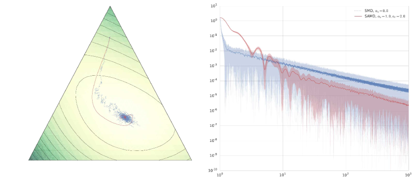
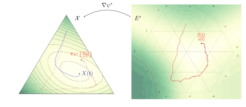
Figure 1: Illustration of SAMD dynamics. The dual trajectory Z​(t)𝑍𝑑Z(t) cumulates negative gradients, Z˙​(t)=βˆ’Ξ·β€‹(t)β€‹βˆ‡f​(X​(t))Λ™π‘π‘‘πœ‚π‘‘βˆ‡π‘“π‘‹π‘‘\dot{Z}(t)=-\eta(t)\nabla f(X(t)). We visualize the scaled dual trajectory Z​(t)/s​(t)𝑍𝑑𝑠𝑑Z(t)/s(t) in the dual space (red), and the corresponding mirror βˆ‡Οˆβˆ—β€‹(Z​(t)s​(t))βˆ‡superscriptπœ“π‘π‘‘π‘ π‘‘\nabla\psi^{*}(\frac{Z(t)}{s(t)}) in the primal space (dotted red). The primal trajectory X​(t)𝑋𝑑X(t) is obtained by averaging the mirror.

We give an illustration of SAMD dynamics in FigureΒ 1, on a simplex-constrained problem in ℝ3superscriptℝ3\mathbb{R}^{3}. The feasible set is given by 𝒳={xβˆˆβ„+n:βˆ‘i=1nxi=1}𝒳conditional-setπ‘₯subscriptsuperscriptℝ𝑛superscriptsubscript𝑖1𝑛subscriptπ‘₯𝑖1\mathcal{X}=\{x\in\mathbb{R}^{n}_{+}:\sum_{i=1}^{n}x_{i}=1\}, and the mirror map is generated by the negative entropy restricted to the simplex, given by:

Οˆβ€‹(x)={βˆ’βˆ‘i=1nxi​ln⁑xiifΒ xβˆˆπ’³,+∞otherwise,πœ“π‘₯casessuperscriptsubscript𝑖1𝑛subscriptπ‘₯𝑖subscriptπ‘₯𝑖ifΒ xβˆˆπ’³,otherwise,\psi(x)=\begin{cases}-\sum_{i=1}^{n}x_{i}\ln x_{i}&\text{if $x\in\mathcal{X}$,}\\ +\infty&\text{otherwise,}\end{cases}

which is strongly convex with respect to the norm βˆ₯β‹…βˆ₯1\|\cdot\|_{1} by Pinsker’s inequality. Its convex conjugate is given by

Οˆβˆ—β€‹(z)=maxxβˆˆπ’³β‘βŸ¨x,zβŸ©βˆ’βˆ‘i=1nxi​ln⁑xi=lnβ€‹βˆ‘i=1nezisuperscriptπœ“π‘§subscriptπ‘₯𝒳π‘₯𝑧superscriptsubscript𝑖1𝑛subscriptπ‘₯𝑖subscriptπ‘₯𝑖superscriptsubscript𝑖1𝑛superscript𝑒subscript𝑧𝑖\displaystyle\psi^{*}(z)=\max_{x\in\mathcal{X}}\left\langle x,z\right\rangle-\sum_{i=1}^{n}x_{i}\ln x_{i}=\ln\sum_{i=1}^{n}e^{z_{i}}

which is differentiable for all z∈Eβˆ—π‘§superscript𝐸z\in E^{*}, and the mirror map is

βˆ‡Οˆβˆ—β€‹(z)=eziβˆ‘j=1nezjβˆˆπ’³βˆ‡superscriptπœ“π‘§superscript𝑒subscript𝑧𝑖superscriptsubscript𝑗1𝑛superscript𝑒subscript𝑧𝑗𝒳\nabla\psi^{*}(z)=\frac{e^{z_{i}}}{\sum_{j=1}^{n}e^{z_{j}}}\in\mathcal{X}

which is Lipschitz w.r.t. the dual norms βˆ₯β‹…βˆ₯1,βˆ₯β‹…βˆ₯∞\|\cdot\|_{1},\|\cdot\|_{\infty}.

Note that for all z∈Eβˆ—π‘§superscript𝐸z\in E^{*} and all Ξ±βˆˆβ„π›Όβ„\alpha\in\mathbb{R},

βˆ‡Οˆβˆ—β€‹(z)=βˆ‡Οˆβˆ—β€‹(z+Ξ±β€‹πŸ),βˆ‡superscriptπœ“π‘§βˆ‡superscriptπœ“π‘§π›Ό1\nabla\psi^{*}(z)=\nabla\psi^{*}(z+\alpha\mathbf{1}),

where 𝟏1\mathbf{1} is the vector of all ones. This can be verified directly using the expression of βˆ‡Οˆβˆ—βˆ‡superscriptπœ“\nabla\psi^{*}, but can also be seen as a consequence of the duality of sub-differentials (e.g. Theorem 23.5 in Rockafellar (1970)), which states that x=βˆ‡Οˆβˆ—β€‹(z)π‘₯βˆ‡superscriptπœ“π‘§x=\nabla\psi^{*}(z) if and only if zβˆˆβˆ‚Οˆβ€‹(x)π‘§πœ“π‘₯z\in\partial\psi(x); and since Οˆπœ“\psi is the restriction of the negative entropy βˆ’H​(x)=βˆ’βˆ‘i=1nxi​ln⁑xi𝐻π‘₯superscriptsubscript𝑖1𝑛subscriptπ‘₯𝑖subscriptπ‘₯𝑖-H(x)=-\sum_{i=1}^{n}x_{i}\ln x_{i} to the simplex, its sub-differential at xπ‘₯x is

βˆ‚Οˆβ€‹(x)=βˆ’βˆ‡H​(x)+n𝒳​(x)πœ“π‘₯βˆ‡π»π‘₯subscript𝑛𝒳π‘₯\partial\psi(x)=-\nabla H(x)+n_{\mathcal{X}}(x)

where n𝒳​(x)subscript𝑛𝒳π‘₯n_{\mathcal{X}}(x) is the normal cone to 𝒳𝒳\mathcal{X} at xπ‘₯x, which is simply the line β„β€‹πŸβ„1\mathbb{R}\mathbf{1} (when xπ‘₯x is in the relative interior of the simplex).

Since the mirror map is constant along the normal to the simplex, we choose to project the dual variable Z𝑍Z on the hyperplane parallel to the simplex, for visualization purposes. This allows us to visualize the relevant component of the dual dynamics, and ignore a component which does not matter for convergence (but which could have high magnitudes if βˆ‡fβˆ‡π‘“\nabla f has a large component along the normal). Note that even numerically, projecting Z𝑍Z after each iteration helps improve numerical stability (without affecting the primal trajectory).

Finally in order to visualize the function values, we generate a triangular mesh of the simplex, then map it to the dual space. In other words, the colors in the primal space represent f​(x)𝑓π‘₯f(x), and in the dual space represent f​(βˆ‡Οˆβˆ—β€‹(z))π‘“βˆ‡superscriptπœ“π‘§f(\nabla\psi^{*}(z)). It is interesting to observe how the mirror map βˆ‡Οˆβˆ—βˆ‡superscriptπœ“\nabla\psi^{*} distorts the space between primal and dual spaces.

The objective function used in this example (which we use as a running numerical example to illustrate our results) is given by the sum of exponentials

f​(x)=βˆ‘i=1ke⟨ci,x⟩,𝑓π‘₯superscriptsubscript𝑖1π‘˜superscript𝑒subscript𝑐𝑖π‘₯f(x)=\sum_{i=1}^{k}e^{\left\langle c_{i},x\right\rangle},

where {ci}1≀i≀ksubscriptsubscript𝑐𝑖1π‘–π‘˜\{c_{i}\}_{1\leq i\leq k} are vectors in ℝnsuperscriptℝ𝑛\mathbb{R}^{n}.

3.2 Existence and uniqueness of a continuous solution

We give the following existence and uniqueness result.

Proposition 2.

Suppose AssumptionsΒ 1, 2 and 3 hold. Then for all T>t0𝑇subscript𝑑0T>t_{0}, SAMDΞ·,a,ssubscriptSAMDπœ‚π‘Žπ‘ \operatorname{SAMD}_{\eta,a,s} has a unique (up to redefinition on a β„™β„™\mathbb{P}-null set) solution (X​(t),Z​(t))𝑋𝑑𝑍𝑑(X(t),Z(t)) continuous on [0,T]0𝑇[0,T], with the property that (X​(t),Z​(t))𝑋𝑑𝑍𝑑(X(t),Z(t)) is adapted to the filtration {β„±t}subscriptℱ𝑑\{\mathcal{F}_{t}\}, and ∫t0Tβ€–X​(t)β€–2​dt,∫t0Tβ€–Z​(t)β€–βˆ—2​𝑑tsuperscriptsubscriptsubscript𝑑0𝑇superscriptnorm𝑋𝑑2subscript𝑑𝑑superscriptsubscriptsubscript𝑑0𝑇superscriptsubscriptnorm𝑍𝑑2differential-d𝑑\int_{t_{0}}^{T}\|X(t)\|^{2}d_{t},\int_{t_{0}}^{T}\|Z(t)\|_{*}^{2}dt have finite expectations.

Proof.

By assumption, βˆ‡Οˆβˆ—βˆ‡superscriptπœ“\nabla\psi^{*} and βˆ‡fβˆ‡π‘“\nabla f are Lipschitz continuous, thus the function (x,z)↦(βˆ’Ξ·β€‹(t)β€‹βˆ‡f​(x),a​(t)​[βˆ‡Οˆβˆ—β€‹(z/s​(t))βˆ’x])maps-toπ‘₯π‘§πœ‚π‘‘βˆ‡π‘“π‘₯π‘Žπ‘‘delimited-[]βˆ‡superscriptπœ“π‘§π‘ π‘‘π‘₯(x,z)\mapsto(-\eta(t)\nabla f(x),a(t)[\nabla\psi^{*}(z/s(t))-x]) is Lipschitz on [t0,T]subscript𝑑0𝑇[t_{0},T] (since a,Ξ·,sπ‘Žπœ‚π‘ a,\eta,s are positive continuous). Additionally, the function x↦σ​(x,t)maps-toπ‘₯𝜎π‘₯𝑑x\mapsto\sigma(x,t) is Lipschitz on the compact set 𝒳𝒳\mathcal{X}. The function Οƒβˆ—β€‹(t)subscriptπœŽπ‘‘\sigma_{*}(t) is continuous, since it is by definition the supremum of continuous functions

Οƒβˆ—2​(t)=supxβˆˆπ’³β€–Ξ£β€‹(x,t)β€–i=supxβˆˆπ’³supβ€–zβ€–βˆ—β‰€1‖Σ​(x,t)​zβ€–superscriptsubscript𝜎2𝑑subscriptsupremumπ‘₯𝒳subscriptnormΞ£π‘₯𝑑𝑖subscriptsupremumπ‘₯𝒳subscriptsupremumsubscriptnorm𝑧1normΞ£π‘₯𝑑𝑧\sigma_{*}^{2}(t)=\sup_{x\in\mathcal{X}}\|\Sigma(x,t)\|_{i}=\sup_{x\in\mathcal{X}}\sup_{\|z\|_{*}\leq 1}\|\Sigma(x,t)z\|

and 𝒳𝒳\mathcal{X} and {z∈Eβˆ—:β€–zβ€–βˆ—β‰€1}conditional-set𝑧superscript𝐸subscriptnorm𝑧1\{z\in E^{*}:\|z\|_{*}\leq 1\} are both compact.

Therefore, we can invoke the existence and uniqueness theorem for stochastic differential equations (Øksendal, 2003, Theorem 5.2.1). ∎

Note that since T𝑇T is arbitrary in the previous proposition, we can conclude that there exists a unique continuous solution on [t0,∞)subscript𝑑0[t_{0},\infty). In the previous proposition, we assumed that 𝒳𝒳\mathcal{X} is compact to guarantee the conditions of the existence and uniqueness theorem, but this can be relaxed. Instead, we can directly assume additional regularity of the noise, e.g. that Σ​(x,t)Ξ£π‘₯𝑑\Sigma(x,t) additionally satisfies ‖Σ​(x,t)β€–i≀C​(1+β€–xβ€–)subscriptnormΞ£π‘₯𝑑𝑖𝐢1normπ‘₯\|\Sigma(x,t)\|_{i}\leq C(1+\|x\|) for some C>0𝐢0C>0, uniformly in t𝑑t.

Next, in order to analyze the convergence properties of the solution trajectories (X​(t),Z​(t))𝑋𝑑𝑍𝑑(X(t),Z(t)), we will need to bound the time-derivative of the energy function L𝐿L.

3.3 Energy decay

In this section, we state and prove two technical lemmas which will be useful in proving our main convergence results. We start by bounding the rate of change of the energy function along solution trajectories of SAMDSAMD\operatorname{SAMD}.

Bounding the rate of change of the energy

Lemma 2.

Suppose AssumptionΒ 1 holds, and that the primal rate satisfies a=Ξ·/rπ‘Žπœ‚π‘Ÿa=\eta/r, and let (X​(t),Z​(t))𝑋𝑑𝑍𝑑(X(t),Z(t)) be a continuous solution to SAMDΞ·,Ξ·/r,ssubscriptSAMDπœ‚πœ‚π‘Ÿπ‘ \operatorname{SAMD}_{\eta,\eta/r,s}. Then for all tβ‰₯t0𝑑subscript𝑑0t\geq t_{0},

d​L𝑑𝐿\displaystyle dL (X​(t),Z​(t),t)≀𝑋𝑑𝑍𝑑𝑑absent\displaystyle(X(t),Z(t),t)\leq
[(f​(X​(t))βˆ’f​(x⋆))​(r˙​(t)βˆ’Ξ·β€‹(t))+Οˆβ€‹(x⋆)​s˙​(t)+n​LΟˆβˆ—2​η2​(t)β€‹Οƒβˆ—2​(t)s​(t)]​d​t+⟨V​(t),d​B​(t)⟩,delimited-[]𝑓𝑋𝑑𝑓superscriptπ‘₯β‹†Λ™π‘Ÿπ‘‘πœ‚π‘‘πœ“superscriptπ‘₯⋆˙𝑠𝑑𝑛subscript𝐿superscriptπœ“2superscriptπœ‚2𝑑superscriptsubscript𝜎2𝑑𝑠𝑑𝑑𝑑𝑉𝑑𝑑𝐡𝑑\displaystyle\left[(f(X(t))-f(x^{\star}))(\dot{r}(t)-\eta(t))+\psi(x^{\star})\dot{s}(t)+\frac{nL_{\psi^{*}}}{2}\frac{\eta^{2}(t)\sigma_{*}^{2}(t)}{s(t)}\right]dt+\left\langle V(t),dB(t)\right\rangle,

where V​(t)𝑉𝑑V(t) is the continuous, n𝑛n dimensional process given by

V​(t)=βˆ’Ξ·β€‹(t)​σ​(X​(t),t)T​(βˆ‡Οˆβˆ—β€‹(Z​(t)/s​(t))βˆ’βˆ‡Οˆβˆ—β€‹(z⋆))π‘‰π‘‘πœ‚π‘‘πœŽsuperscriptπ‘‹π‘‘π‘‘π‘‡βˆ‡superscriptπœ“π‘π‘‘π‘ π‘‘βˆ‡superscriptπœ“superscript𝑧⋆V(t)=-\eta(t)\sigma(X(t),t)^{T}(\nabla\psi^{*}(Z(t)/s(t))-\nabla\psi^{*}(z^{\star})) (16)
Proof.

By definition of the energy function L𝐿L, βˆ‡xL​(x,z,t)=r​(t)β€‹βˆ‡f​(x)subscriptβˆ‡π‘₯𝐿π‘₯π‘§π‘‘π‘Ÿπ‘‘βˆ‡π‘“π‘₯\nabla_{x}L(x,z,t)=r(t)\nabla f(x) and βˆ‡zL​(x,z,t)=βˆ‡Οˆβˆ—β€‹(z/s​(t))βˆ’βˆ‡Οˆβˆ—β€‹(z⋆)subscriptβˆ‡π‘§πΏπ‘₯π‘§π‘‘βˆ‡superscriptπœ“π‘§π‘ π‘‘βˆ‡superscriptπœ“superscript𝑧⋆\nabla_{z}L(x,z,t)=\nabla\psi^{*}(z/s(t))-\nabla\psi^{*}(z^{\star}), which are Lipschitz continuous in (x,z)π‘₯𝑧(x,z) (uniformly in t𝑑t on any bounded interval, since s​(t),r​(t)π‘ π‘‘π‘Ÿπ‘‘s(t),r(t) are continuous positive functions of t𝑑t). Thus by the ItΓ΄ formula for functions with Lipschitz continuous gradientsΒ (Errami etΒ al., 2002), we have

d​L𝑑𝐿\displaystyle dL =βˆ‚tL​d​t+βŸ¨βˆ‡xL,d​X⟩+βŸ¨βˆ‡zL,d​Z⟩+12​tr⁑(η​σTβ€‹βˆ‡z​z2L​σ​η)​d​tabsentsubscript𝑑𝐿𝑑𝑑subscriptβˆ‡π‘₯𝐿𝑑𝑋subscriptβˆ‡π‘§πΏπ‘‘π‘12trπœ‚superscriptπœŽπ‘‡subscriptsuperscriptβˆ‡2π‘§π‘§πΏπœŽπœ‚π‘‘π‘‘\displaystyle=\partial_{t}Ldt+\left\langle\nabla_{x}L,dX\right\rangle+\left\langle\nabla_{z}L,dZ\right\rangle+\frac{1}{2}\operatorname{tr}\left(\eta\sigma^{T}\nabla^{2}_{zz}L\sigma\eta\right)dt
=βˆ‚tL​d​t+βŸ¨βˆ‡xL,d​X⟩+βŸ¨βˆ‡zL,βˆ’Ξ·β€‹βˆ‡f​(X)βŸ©β€‹d​t+βŸ¨βˆ‡zL,βˆ’Ξ·β€‹Οƒβ€‹d​B⟩+Ξ·22​tr⁑(Ξ£β€‹βˆ‡z​z2L)​d​t.absentsubscript𝑑𝐿𝑑𝑑subscriptβˆ‡π‘₯𝐿𝑑𝑋subscriptβˆ‡π‘§πΏπœ‚βˆ‡π‘“π‘‹π‘‘π‘‘subscriptβˆ‡π‘§πΏπœ‚πœŽπ‘‘π΅superscriptπœ‚22trΞ£subscriptsuperscriptβˆ‡2𝑧𝑧𝐿𝑑𝑑\displaystyle=\partial_{t}Ldt+\left\langle\nabla_{x}L,dX\right\rangle+\left\langle\nabla_{z}L,-\eta\nabla f(X)\right\rangle dt+\left\langle\nabla_{z}L,-\eta\sigma dB\right\rangle+\frac{\eta^{2}}{2}\operatorname{tr}\left(\Sigma\nabla^{2}_{zz}L\right)dt.

The first three terms correspond exactly to the deterministic case, and we can bound them byΒ (21) from LemmaΒ 1. The last two terms are due to the stochastic noise, and consist of a volatility term

βˆ’Ξ·β€‹βŸ¨βˆ‡zL​(X,Z,t),σ​d​B⟩=βˆ’Ξ·β€‹βŸ¨βˆ‡Οˆβˆ—β€‹(Z/s)βˆ’βˆ‡Οˆβˆ—β€‹(z⋆),σ​d​B⟩=⟨V,d​B⟩,πœ‚subscriptβˆ‡π‘§πΏπ‘‹π‘π‘‘πœŽπ‘‘π΅πœ‚βˆ‡superscriptπœ“π‘π‘ βˆ‡superscriptπœ“superscriptπ‘§β‹†πœŽπ‘‘π΅π‘‰π‘‘π΅-\eta\left\langle\nabla_{z}L(X,Z,t),\sigma dB\right\rangle=-\eta\left\langle\nabla\psi^{*}(Z/s)-\nabla\psi^{*}(z^{\star}),\sigma dB\right\rangle=\left\langle V,dB\right\rangle,

and the ItΓ΄ correction term

Ξ·22​tr⁑(Σ​(X,t)β€‹βˆ‡z​z2L​(X,Z,t))​d​t=Ξ·22​s​tr⁑(Σ​(X,t)β€‹βˆ‡2Οˆβˆ—β€‹(Z/s))​d​t.superscriptπœ‚22trΣ𝑋𝑑subscriptsuperscriptβˆ‡2𝑧𝑧𝐿𝑋𝑍𝑑𝑑𝑑superscriptπœ‚22𝑠trΣ𝑋𝑑superscriptβˆ‡2superscriptπœ“π‘π‘ π‘‘π‘‘\frac{\eta^{2}}{2}\operatorname{tr}\left(\Sigma(X,t)\nabla^{2}_{zz}L(X,Z,t)\right)dt=\frac{\eta^{2}}{2s}\operatorname{tr}\left(\Sigma(X,t)\nabla^{2}\psi^{*}(Z/s)\right)dt.

We can bound the last term using the following simple fact: Given two linear operators P:Eβ†’Eβˆ—:𝑃→𝐸superscript𝐸P:E\to E^{*} and Q:Eβˆ—β†’E:𝑄→superscript𝐸𝐸Q:E^{*}\to E, such that β€–Pβ€–βˆ—,i≀αPsubscriptnorm𝑃𝑖subscript𝛼𝑃\|P\|_{*,i}\leq\alpha_{P} and β€–Qβ€–i≀αQsubscriptnorm𝑄𝑖subscript𝛼𝑄\|Q\|_{i}\leq\alpha_{Q} (where βˆ₯β‹…βˆ₯i\|\cdot\|_{i} and βˆ₯β‹…βˆ₯βˆ—,i\|\cdot\|_{*,i} are the norms induced by the pair of dual norms βˆ₯β‹…βˆ₯\|\cdot\| and βˆ₯β‹…βˆ₯βˆ—\|\cdot\|_{*}), then we have tr⁑(P​Q)≀n​αP​αQtr𝑃𝑄𝑛subscript𝛼𝑃subscript𝛼𝑄\operatorname{tr}(PQ)\leq n\alpha_{P}\alpha_{Q} since

tr⁑(P​Q)=βˆ‘j=1n⟨Pj,QjβŸ©β‰€βˆ‘j=1nβ€–Pjβ€–βˆ—β€‹β€–Qjβ€–β‰€βˆ‘j=1nβ€–Pβ€–βˆ—,i​‖Qβ€–βˆ—,i.tr𝑃𝑄superscriptsubscript𝑗1𝑛subscript𝑃𝑗subscript𝑄𝑗superscriptsubscript𝑗1𝑛subscriptnormsubscript𝑃𝑗normsubscript𝑄𝑗superscriptsubscript𝑗1𝑛subscriptnorm𝑃𝑖subscriptnorm𝑄𝑖\displaystyle\operatorname{tr}(PQ)=\sum_{j=1}^{n}\left\langle P_{j},Q_{j}\right\rangle\leq\sum_{j=1}^{n}\|P_{j}\|_{*}\|Q_{j}\|\leq\sum_{j=1}^{n}\|P\|_{*,i}\|Q\|_{*,i}.

Now, since βˆ‡Οˆβˆ—βˆ‡superscriptπœ“\nabla\psi^{*} is, by assumption, LΟˆβˆ—subscript𝐿superscriptπœ“L_{\psi^{*}}-Lipschitz, we have β€–βˆ‡Οˆβˆ—β€–i≀LΟˆβˆ—subscriptnormβˆ‡superscriptπœ“π‘–subscript𝐿superscriptπœ“\|\nabla\psi^{*}\|_{i}\leq L_{\psi^{*}}, and by definitionΒ (15) ofΒ Οƒβˆ—superscript𝜎\sigma^{*}, ‖Σ​(x,t)β€–βˆ—β‰€Οƒβˆ—2​(t)subscriptnormΞ£π‘₯𝑑superscriptsubscript𝜎2𝑑\|\Sigma(x,t)\|_{*}\leq\sigma_{*}^{2}(t) for all xπ‘₯x, therefore for all x∈Eπ‘₯𝐸x\in E, z∈Eβˆ—π‘§superscript𝐸z\in E^{*}, and tβ‰₯t0𝑑subscript𝑑0t\geq t_{0},

tr⁑(Σ​(x,t)β€‹βˆ‡2Οˆβˆ—β€‹(z))≀n​LΟˆβˆ—β€‹Οƒβˆ—2​(t).trΞ£π‘₯𝑑superscriptβˆ‡2superscriptπœ“π‘§π‘›subscript𝐿superscriptπœ“superscriptsubscript𝜎2𝑑\operatorname{tr}(\Sigma(x,t)\nabla^{2}\psi^{*}(z))\leq nL_{\psi^{*}}\sigma_{*}^{2}(t).

Combining the previous inequalities, we obtain the desired bound. ∎

Comparing the bound of LemmaΒ 2 to its deterministic counterpart of LemmaΒ 1, we can see that in the stochastic case, we have two additional terms: a drift term proportional to Οƒβˆ—2​(t)superscriptsubscript𝜎2𝑑\sigma_{*}^{2}(t), which is due to the ItΓ΄ correction term, and a volatility term given by ⟨V​(t),d​B​(t)βŸ©π‘‰π‘‘π‘‘π΅π‘‘\left\langle V(t),dB(t)\right\rangle.

To illustrate these terms, we generate solution trajectories for the sum-exponential example of SectionΒ 3.1, for both the deterministic and stochastic dynamics, and plot the values of the objective function and the energy function. For simplicity, we consider a constant volatility σ​(x,t)=Οƒ0=.1𝜎π‘₯𝑑subscript𝜎0.1\sigma(x,t)=\sigma_{0}=.1, a linear energy rate r​(t)=tπ‘Ÿπ‘‘π‘‘r(t)=t, and a sensitivity 1s​(t)=1t1𝑠𝑑1𝑑\frac{1}{s(t)}=\frac{1}{\sqrt{t}}. The primal and dual weights are η​(t)=r˙​(t)=1πœ‚π‘‘Λ™π‘Ÿπ‘‘1\eta(t)=\dot{r}(t)=1 and a​(t)=η​(t)r​(t)=1tπ‘Žπ‘‘πœ‚π‘‘π‘Ÿπ‘‘1𝑑a(t)=\frac{\eta(t)}{r(t)}=\frac{1}{t}. For the stochastic dynamics, we plot the mean and standard deviation of 100100100 sample trajectories. The results are given in FigureΒ 2 below.

Refer to caption
Figure 2: Illustration of the differences between the deterministic and stochastic variants of accelerated mirror descent dynamics. The right plot shows the values of the objective function f​(X​(t))βˆ’f​(x⋆)𝑓𝑋𝑑𝑓superscriptπ‘₯⋆f(X(t))-f(x^{\star}) (solid lines) and the energy function L​(X​(t),Z​(t),t)𝐿𝑋𝑑𝑍𝑑𝑑L(X(t),Z(t),t) (dashed lines) as a function of t𝑑t. For the stochastic dynamics, we generate 100100100 sample trajectories and plot the mean and standard deviation. The difference in mean energy values illustrates the drift term (captured by the ItΓ΄ correction term), and the standard deviation illustrates the volatility term. We also plot the primal and dual trajectories (for a single sample) in the left and center figures, respectively.
Refer to caption
Figure 3: Illustration of the differences between the deterministic and stochastic variants of (non-accelerated) mirror descent dynamics. The stochastic dynamics exhibit a slower convergence rate.

For the sake of comparison, we also generate a similar simulation for (non-accelerated) mirror descent dynamics in FigureΒ 3, using the same sensitivity 1s​(t)=1t1𝑠𝑑1𝑑\frac{1}{s(t)}=\frac{1}{\sqrt{t}}. Comparing FiguresΒ 2 andΒ 3, we can already observe some qualitative differences introduced by acceleration: the accelerated dynamics exhibit faster convergence, accompanied with typical oscillations around the minimizer. Note that these oscillations are not due to discretization or noise in the gradient estimate (as can be observed e.g. in discrete gradient descent with large step sizes). The oscillations are rather a property of the continuous-time accelerated dynamics. Besides, acceleration also seems to reduce the effect of noise on the primal trajectory (which appears visually smoother than its non-accelerated counterpart). To give some intuition, consider the following informal argument (which will be formalized in the results of SectionΒ 4). In the case of mirror descent, the primal variable is obtained as the mirror of Z​(t)/s​(t)𝑍𝑑𝑠𝑑Z(t)/s(t), where

Z​(t)s​(t)=βˆ’1s​(t)β€‹βˆ«t0tβˆ‡f​(X​(Ο„))​𝑑τ+1s​(t)β€‹βˆ«t0tσ​(X​(Ο„),Ο„)​𝑑B​(Ο„),𝑍𝑑𝑠𝑑1𝑠𝑑superscriptsubscriptsubscript𝑑0π‘‘βˆ‡π‘“π‘‹πœdifferential-d𝜏1𝑠𝑑superscriptsubscriptsubscript𝑑0π‘‘πœŽπ‘‹πœπœdifferential-d𝐡𝜏\displaystyle\frac{Z(t)}{s(t)}=-\frac{1}{s(t)}\int_{t_{0}}^{t}\nabla f(X(\tau))d\tau+\frac{1}{s(t)}\int_{t_{0}}^{t}\sigma(X(\tau),\tau)dB(\tau),

and the noise is cumulated in the ItΓ΄ martingale term ∫t0tσ​(X​(Ο„),Ο„)​𝑑B​(Ο„)superscriptsubscriptsubscript𝑑0π‘‘πœŽπ‘‹πœπœdifferential-d𝐡𝜏\int_{t_{0}}^{t}\sigma(X(\tau),\tau)dB(\tau). In the case of accelerated mirror descent, there are two main differences:

  1. 1.

    First, using a time-varying dual rate η​(t)πœ‚π‘‘\eta(t) in SAMDSAMD\operatorname{SAMD} leads to a non-linear accumulation of noise in the ItΓ΄ martingale ∫t0tη​(Ο„)​σ​(X​(Ο„),Ο„)​𝑑B​(Ο„)superscriptsubscriptsubscript𝑑0π‘‘πœ‚πœπœŽπ‘‹πœπœdifferential-d𝐡𝜏\int_{t_{0}}^{t}\eta(\tau)\sigma(X(\tau),\tau)dB(\tau).

  2. 2.

    Second, due to the averaging in the primal space (given by the integralΒ (6)), the smaller noise in the past trajectory results in a smaller noise of the weighted average (similarly to acceleration by averaging ofΒ Polyak and Juditsky (1992) in discrete time).

The combined effect of averaging in the dual space (using η​(t)πœ‚π‘‘\eta(t)) and in the primal space (using a​(t)π‘Žπ‘‘a(t)) will be apparent in SectionΒ 4 when we derive explicit convergence rates.

Bounding the ItΓ΄ martingale term

Integrating the bound of LemmaΒ 2 will allow us to bound changes in energy. This bound will involve the ItΓ΄ martingale ∫t0t⟨V​(Ο„),d​B​(Ο„)⟩superscriptsubscriptsubscript𝑑0π‘‘π‘‰πœπ‘‘π΅πœ\int_{t_{0}}^{t}\left\langle V(\tau),dB(\tau)\right\rangle, where V𝑉V is defined inΒ (16). In order to control this term, we give, in the following lemma, an asymptotic envelope (a consequence of the law of the iterated logarithm).

Lemma 3.

Suppose AssumptionsΒ 2 and 3 hold. Let b​(t)=∫t0tΞ·2​(Ο„)β€‹Οƒβˆ—2​(Ο„)​𝑑τ𝑏𝑑superscriptsubscriptsubscript𝑑0𝑑superscriptπœ‚2𝜏superscriptsubscript𝜎2𝜏differential-d𝜏b(t)=\int_{t_{0}}^{t}\eta^{2}(\tau)\sigma_{*}^{2}(\tau)d\tau. Then

∫t0t⟨V​(Ο„),d​B​(Ο„)⟩=π’ͺ​(b​(t)​log⁑log⁑b​(t))superscriptsubscriptsubscript𝑑0π‘‘π‘‰πœπ‘‘π΅πœπ’ͺ𝑏𝑑𝑏𝑑\displaystyle\int_{t_{0}}^{t}\left\langle V(\tau),dB(\tau)\right\rangle=\mathcal{O}(\sqrt{b(t)\log\log b(t)}) a.s. asΒ tβ†’βˆž.a.s. asΒ tβ†’βˆž\displaystyle\text{a.s. as $t\to\infty$}. (17)
Proof.

Let us denote the ItΓ΄ martingale by 𝒱​(t)=∫t0t⟨V​(Ο„),d​B​(Ο„)⟩=βˆ‘i=1n∫t0tVi​(Ο„)​𝑑Bi​(Ο„)𝒱𝑑superscriptsubscriptsubscript𝑑0π‘‘π‘‰πœπ‘‘π΅πœsuperscriptsubscript𝑖1𝑛superscriptsubscriptsubscript𝑑0𝑑subscriptπ‘‰π‘–πœdifferential-dsubscriptπ΅π‘–πœ\mathcal{V}(t)=\int_{t_{0}}^{t}\left\langle V(\tau),dB(\tau)\right\rangle=\sum_{i=1}^{n}\int_{t_{0}}^{t}V_{i}(\tau)dB_{i}(\tau), and its quadratic variation by β​(t)=[𝒱​(t),𝒱​(t)]𝛽𝑑𝒱𝑑𝒱𝑑\beta(t)=[\mathcal{V}(t),\mathcal{V}(t)]. By definition of 𝒱𝒱\mathcal{V}, we have

d​β=βˆ‘i=1nβˆ‘j=1nVi​Vj​d​[Bi,Bj]=βˆ‘i=1nVi2​d​t=⟨V,VβŸ©β€‹d​t.𝑑𝛽superscriptsubscript𝑖1𝑛superscriptsubscript𝑗1𝑛subscript𝑉𝑖subscript𝑉𝑗𝑑subscript𝐡𝑖subscript𝐡𝑗superscriptsubscript𝑖1𝑛superscriptsubscript𝑉𝑖2𝑑𝑑𝑉𝑉𝑑𝑑d\beta=\sum_{i=1}^{n}\sum_{j=1}^{n}V_{i}V_{j}d[B_{i},B_{j}]=\sum_{i=1}^{n}V_{i}^{2}dt=\left\langle V,V\right\rangle dt.

By the Dambis-Dubins-Schwartz time change theorem (e.g. Corollary 8.5.4 in (Øksendal, 2003)), there exists a Wiener process B^^𝐡\hat{B} such that

𝒱​(t)=B^​(β​(t)).𝒱𝑑^𝐡𝛽𝑑\mathcal{V}(t)=\hat{B}(\beta(t)). (18)

We now proceed to bound β​(t)𝛽𝑑\beta(t). Using the expressionΒ (16) of V𝑉V, we have

⟨V,V⟩=Ξ·2​(t)​ΔT​(t)​Σ​(X,t)​Δ​(t),𝑉𝑉superscriptπœ‚2𝑑superscriptΔ𝑇𝑑Σ𝑋𝑑Δ𝑑\left\langle V,V\right\rangle=\eta^{2}(t)\Delta^{T}(t)\Sigma(X,t)\Delta(t),

where we defined Δ​(t)=βˆ‡Οˆβˆ—β€‹(Z​(t)/s​(t))βˆ’βˆ‡Οˆβˆ—β€‹(z⋆)Ξ”π‘‘βˆ‡superscriptπœ“π‘π‘‘π‘ π‘‘βˆ‡superscriptπœ“superscript𝑧⋆\Delta(t)=\nabla\psi^{*}(Z(t)/s(t))-\nabla\psi^{*}(z^{\star}). Since the mirror map has values in 𝒳𝒳\mathcal{X} and 𝒳𝒳\mathcal{X} is assumed compact, the diameter D=supx,xβ€²βˆˆπ’³β€–xβˆ’x′‖𝐷subscriptsupremumπ‘₯superscriptπ‘₯′𝒳normπ‘₯superscriptπ‘₯β€²D=\sup_{x,x^{\prime}\in\mathcal{X}}\|x-x^{\prime}\| is finite, and Δ​(t)≀DΔ𝑑𝐷\Delta(t)\leq D for all t𝑑t. Thus, d​β​(t)≀D2​η​(t)2β€‹Οƒβˆ—2​(t)​d​t𝑑𝛽𝑑superscript𝐷2πœ‚superscript𝑑2superscriptsubscript𝜎2𝑑𝑑𝑑d\beta(t)\leq D^{2}\eta(t)^{2}\sigma_{*}^{2}(t)dt, and integrating,

β​(t)≀D2​b​(t)𝛽𝑑superscript𝐷2𝑏𝑑\displaystyle\beta(t)\leq D^{2}b(t) Β Β a.s. (19)

Since β​(t)𝛽𝑑\beta(t) is a non-decreasing process, two cases are possible: if limtβ†’βˆžΞ²β€‹(t)subscript→𝑑𝛽𝑑\lim_{t\to\infty}\beta(t) is finite, then lim suptβ†’βˆž|𝒱​(t)|subscriptlimit-supremum→𝑑𝒱𝑑\limsup_{t\to\infty}|\mathcal{V}(t)| is a.s. finite and the result follows immediately. If limtβ†’βˆžΞ²β€‹(t)=∞subscript→𝑑𝛽𝑑\lim_{t\to\infty}\beta(t)=\infty, then

lim suptβ†’βˆžπ’±β€‹(t)b​(t)​log⁑log⁑b​(t)≀lim suptβ†’βˆžB^​(β​(t))β​(t)D2​log⁑log⁑β​(t)D2=D​2subscriptlimit-supremum→𝑑𝒱𝑑𝑏𝑑𝑏𝑑subscriptlimit-supremum→𝑑^𝐡𝛽𝑑𝛽𝑑superscript𝐷2𝛽𝑑superscript𝐷2𝐷2\displaystyle\limsup_{t\to\infty}\frac{\mathcal{V}(t)}{\sqrt{b(t)\log\log b(t)}}\leq\limsup_{t\to\infty}\frac{\hat{B}(\beta(t))}{\sqrt{\frac{\beta(t)}{D^{2}}\log\log\frac{\beta(t)}{D^{2}}}}=D\sqrt{2} a.s.

where the inequality combines (18) and (19), and the equality is by the law of the iterated logarithm. ∎

4 Convergence results

4.1 Almost sure convergence

Equipped with LemmaΒ 2 and LemmaΒ 3, which bound, respectively, the rate of change of the energy and the asymptotic growth of the martingale term, we are now ready to prove our convergence results.

Theorem 1.

Suppose that AssumptionsΒ 1, 2, and 3 hold. Suppose that η​(t)β€‹Οƒβˆ—β€‹(t)=o​(1/log⁑t)πœ‚π‘‘subscriptπœŽπ‘‘π‘œ1𝑑\eta(t)\sigma_{*}(t)=o(1/\sqrt{\log t}), and that ∫t0tη​(Ο„)​𝑑τsuperscriptsubscriptsubscript𝑑0π‘‘πœ‚πœdifferential-d𝜏\int_{t_{0}}^{t}\eta(\tau)d\tau dominates b​(t)𝑏𝑑b(t) and b​(t)​log⁑log⁑b​(t)𝑏𝑑𝑏𝑑\sqrt{b(t)\log\log b(t)} (where b​(t)=∫t0tΞ·2​(Ο„)β€‹Οƒβˆ—2​(Ο„)​𝑑τ𝑏𝑑superscriptsubscriptsubscript𝑑0𝑑superscriptπœ‚2𝜏superscriptsubscript𝜎2𝜏differential-d𝜏b(t)=\int_{t_{0}}^{t}\eta^{2}(\tau)\sigma_{*}^{2}(\tau)d\tau as defined in LemmaΒ 3). Consider SAMDSAMD\operatorname{SAMD} dynamics with r=s=1π‘Ÿπ‘ 1r=s=1 and a=Ξ·π‘Žπœ‚a=\eta. Let (X​(t),Z​(t))𝑋𝑑𝑍𝑑(X(t),Z(t)) be the unique continuous solution of SAMDΞ·,Ξ·,1subscriptSAMDπœ‚πœ‚1\operatorname{SAMD}_{\eta,\eta,1}. Then

limtβ†’βˆžf​(X​(t))βˆ’f​(x⋆)=0subscript→𝑑𝑓𝑋𝑑𝑓superscriptπ‘₯⋆0\displaystyle\lim_{t\to\infty}f(X(t))-f(x^{\star})=0 a.s.

The result of TheoremΒ 1 makes it possible to guarantee almost sure convergence (albeit without an explicit convergence rate) when the noise is persistent (Οƒβˆ—β€‹(t)subscriptπœŽπ‘‘\sigma_{*}(t) is constant, or even increasing). To give a concrete example, suppose Οƒβˆ—β€‹(t)=π’ͺ​(tΞ±)subscriptπœŽπ‘‘π’ͺsuperscript𝑑𝛼\sigma_{*}(t)=\mathcal{O}(t^{\alpha}) (with Ξ±<12𝛼12\alpha<\frac{1}{2} but can be positive), and let η​(t)=tβˆ’Ξ±βˆ’12πœ‚π‘‘superscript𝑑𝛼12\eta(t)=t^{-\alpha-\frac{1}{2}}. Then η​(t)β€‹Οƒβˆ—β€‹(t)=π’ͺ​(tβˆ’12)πœ‚π‘‘subscriptπœŽπ‘‘π’ͺsuperscript𝑑12\eta(t)\sigma_{*}(t)=\mathcal{O}(t^{-\frac{1}{2}}), ∫t0tη​(Ο„)​𝑑τ=Ω​(tβˆ’Ξ±+12)superscriptsubscriptsubscript𝑑0π‘‘πœ‚πœdifferential-d𝜏Ωsuperscript𝑑𝛼12\int_{t_{0}}^{t}\eta(\tau)d\tau=\Omega(t^{-\alpha+\frac{1}{2}}), b​(t)=π’ͺ​(log⁑t)𝑏𝑑π’ͺ𝑑b(t)=\mathcal{O}(\log t), and b​(t)​log⁑log⁑b​(t)=π’ͺ​(log⁑t​log⁑log⁑log⁑t)𝑏𝑑𝑏𝑑π’ͺ𝑑𝑑\sqrt{b(t)\log\log b(t)}=\mathcal{O}(\sqrt{\log t\log\log\log t}), and the conditions of the theorem are satisfied. Therefore, with the appropriate choice of learning rate η​(t)πœ‚π‘‘\eta(t) (and the corresponding averaging in the primal space given by a​(t)=η​(t)π‘Žπ‘‘πœ‚π‘‘a(t)=\eta(t)), one can recover almost sure convergence.

We start by giving an outline of the proof, which is similar to that of TheoremΒ 4.1 in (Mertikopoulos and Staudigl, 2016), with some significant changes (we do not make the assumption that the minimizer is unique, and most importantly, the dynamics and the energy function are different, since averaging is essential in our case to handle the noise, since we do not assume that the volatility bound Οƒβˆ—β€‹(t)subscriptπœŽπ‘‘\sigma_{*}(t) is vanishing). The argument proceeds in the following steps:

  1. (i)

    The first step is to prove that under the conditions of the theorem, the continuous solution of SAMDΞ·,Ξ·,1subscriptSAMDπœ‚πœ‚1\operatorname{SAMD}_{\eta,\eta,1}, (X​(t),Z​(t))𝑋𝑑𝑍𝑑(X(t),Z(t)), is an asymptotic pseudo trajectory (a notion defined and studied byΒ BenaΓ―m and Hirsch (1996) and BenaΓ―m (1999)) of the deterministic flow AMDΞ·,Ξ·,1subscriptAMDπœ‚πœ‚1\operatorname{AMD}_{\eta,\eta,1}. The definition is given below, but intuitively, this means that for large enough times, the sample paths of the process (X​(t),Z​(t))𝑋𝑑𝑍𝑑(X(t),Z(t)) get arbitrarily close to (x​(t),z​(t))π‘₯𝑑𝑧𝑑(x(t),z(t)), the solution trajectories of the deterministic dynamics.

    Definition 4.1 (Asymptotic Pseudo Trajectory).

    Let Ξ¦t:𝒳×Eβˆ—β†’π’³Γ—Eβˆ—:subscriptΦ𝑑→𝒳superscript𝐸𝒳superscript𝐸\Phi_{t}:\mathcal{X}\times E^{*}\to\mathcal{X}\times E^{*} be the semi-flow associated to the deterministic dynamics AMDΞ·,Ξ·,1subscriptAMDπœ‚πœ‚1\operatorname{AMD}_{\eta,\eta,1}, that is, (x​(t),z​(t))=Ξ¦t​(x0,z0)π‘₯𝑑𝑧𝑑subscriptΦ𝑑subscriptπ‘₯0subscript𝑧0(x(t),z(t))=\Phi_{t}(x_{0},z_{0}) is the solution of the deterministic dynamics AMDΞ·,Ξ·,1subscriptAMDπœ‚πœ‚1\operatorname{AMD}_{\eta,\eta,1} with initial condition (x0,z0)subscriptπ‘₯0subscript𝑧0(x_{0},z_{0}). A continuous function t↦(X​(t),Z​(t))βˆˆπ’³Γ—Eβˆ—maps-to𝑑𝑋𝑑𝑍𝑑𝒳superscript𝐸t\mapsto(X(t),Z(t))\in\mathcal{X}\times E^{*} is an asymptotic pseudo trajectory (APT) for Ξ¦tsubscriptΦ𝑑\Phi_{t} if for all T>0𝑇0T>0,

    limtβ†’βˆžsup0≀h≀Td​((X​(t+h),Z​(t+h)),Ξ¦h​(X​(t),Z​(t)))=0,subscript→𝑑subscriptsupremum0β„Žπ‘‡π‘‘π‘‹π‘‘β„Žπ‘π‘‘β„ŽsubscriptΞ¦β„Žπ‘‹π‘‘π‘π‘‘0\lim_{t\to\infty}\sup_{0\leq h\leq T}d((X(t+h),Z(t+h)),\Phi_{h}(X(t),Z(t)))=0,

    where d𝑑d is a distance on 𝒳×Eβˆ—π’³superscript𝐸\mathcal{X}\times E^{*}, e.g. d​((x,z),(xβ€²,zβ€²))=β€–xβˆ’xβ€²β€–+β€–zβˆ’zβ€²β€–βˆ—π‘‘π‘₯𝑧superscriptπ‘₯β€²superscript𝑧′normπ‘₯superscriptπ‘₯β€²subscriptnorm𝑧superscript𝑧′d((x,z),(x^{\prime},z^{\prime}))=\|x-x^{\prime}\|+\|z-z^{\prime}\|_{*}.

  2. (ii)

    The second step is to show that under the deterministic flow, the energy L𝐿L decreases enough for large enough times.

  3. (iii)

    The third step is to prove that under the stochastic process, f​(X​(t))𝑓𝑋𝑑f(X(t)) cannot stay bounded away from f​(x⋆)𝑓superscriptπ‘₯⋆f(x^{\star}) for allΒ t𝑑t.

Finally, combining these steps, we argue that by (iii), f​(X​(t))𝑓𝑋𝑑f(X(t)) eventually gets close to f​(x⋆)𝑓superscriptπ‘₯⋆f(x^{\star}), then stays close by virtue of the asymptotic pseudo trajectory property (i), and the decrease of the energy under the deterministic flow (ii).

Proof of TheoremΒ 1.

We start by specializing the energy function and the bounds on its time derivative to the setting of TheoremΒ 1. Under the assumptions of the theorem (r​(t)=s​(t)=1π‘Ÿπ‘‘π‘ π‘‘1r(t)=s(t)=1), L​(x,z,t)𝐿π‘₯𝑧𝑑L(x,z,t) simplifies to

Lz⋆​(x,z)=f​(x)βˆ’f​(x⋆)+DΟˆβˆ—β€‹(z,z⋆),subscript𝐿superscript𝑧⋆π‘₯𝑧𝑓π‘₯𝑓superscriptπ‘₯⋆subscript𝐷superscriptπœ“π‘§superscript𝑧⋆L_{z^{\star}}(x,z)=f(x)-f(x^{\star})+D_{\psi^{*}}(z,z^{\star}),

where we added the subscript z⋆subscript𝑧⋆z_{\star} to insist on the fact that the energy function is β€œanchored” at z⋆superscript𝑧⋆z^{\star}. Note that since the minimizer is not necessarily unique, Lz⋆​(x​(t),z​(t))subscript𝐿superscript𝑧⋆π‘₯𝑑𝑧𝑑L_{z^{\star}}(x(t),z(t)) does not necessarily converge to 00 for arbitrary z⋆superscript𝑧⋆z^{\star}. Thus, we define and use

L¯​(x,z)=infzβ‹†βˆˆπ’΅β‹†Lz⋆​(x,z),¯𝐿π‘₯𝑧subscriptinfimumsuperscript𝑧⋆superscript𝒡⋆subscript𝐿superscript𝑧⋆π‘₯𝑧\bar{L}(x,z)=\inf_{z^{\star}\in\mathcal{Z}^{\star}}L_{z^{\star}}(x,z),

where 𝒡⋆={z∈Eβˆ—:βˆ‡Οˆβˆ—β€‹(z⋆)βˆˆπ’³β‹†}=βˆͺxβ‹†βˆˆπ’³β‹†βˆ‚Οˆβ€‹(x⋆)superscript𝒡⋆conditional-set𝑧superscriptπΈβˆ‡superscriptπœ“superscript𝑧⋆superscript𝒳⋆subscriptsuperscriptπ‘₯⋆superscriptπ’³β‹†πœ“superscriptπ‘₯⋆\mathcal{Z}^{\star}=\{z\in E^{*}:\nabla\psi^{*}(z^{\star})\in\mathcal{X}^{\star}\}=\cup_{x^{\star}\in\mathcal{X}^{\star}}\partial\psi(x^{\star}) (by the fact that xβ‹†βˆˆβˆ‚Οˆβˆ—β€‹(z⋆)superscriptπ‘₯⋆superscriptπœ“superscript𝑧⋆x^{\star}\in\partial\psi^{*}(z^{\star}) if and only if zβ‹†βˆˆβˆ‚Οˆβ€‹(x⋆)superscriptπ‘§β‹†πœ“superscriptπ‘₯⋆z^{\star}\in\partial\psi(x^{\star})).

Next, we observe that since βˆ‡fβˆ‡π‘“\nabla f is Lfsubscript𝐿𝑓L_{f}-Lipschitz and βˆ‡Οˆβˆ—βˆ‡superscriptπœ“\nabla\psi^{*} is LΟˆβˆ—subscript𝐿superscriptπœ“L_{\psi^{*}}-Lipschitz, we can bound the change of the energy due to small displacements in (x,z)π‘₯𝑧(x,z): we will use the fact that for any convex function f𝑓f with L𝐿L-Lipschitz gradient, f​(x+Ξ΄x)≀f​(x)+βŸ¨βˆ‡f​(x),Ξ΄x⟩+L2​‖δxβ€–2𝑓π‘₯subscript𝛿π‘₯𝑓π‘₯βˆ‡π‘“π‘₯subscript𝛿π‘₯𝐿2superscriptnormsubscript𝛿π‘₯2f(x+\delta_{x})\leq f(x)+\left\langle\nabla f(x),\delta_{x}\right\rangle+\frac{L}{2}\|\delta_{x}\|^{2}. We have

Lz⋆subscript𝐿superscript𝑧⋆\displaystyle L_{z^{\star}} (x+Ξ΄x,z+Ξ΄z)π‘₯subscript𝛿π‘₯𝑧subscript𝛿𝑧\displaystyle(x+\delta_{x},z+\delta_{z})
=f​(x+Ξ΄x)βˆ’f​(x⋆)+Οˆβˆ—β€‹(z+Ξ΄z)βˆ’Οˆβˆ—β€‹(z⋆)βˆ’βŸ¨βˆ‡Οˆβˆ—β€‹(z⋆),z+δ​zβˆ’zβ‹†βŸ©absent𝑓π‘₯subscript𝛿π‘₯𝑓superscriptπ‘₯⋆superscriptπœ“π‘§subscript𝛿𝑧superscriptπœ“superscriptπ‘§β‹†βˆ‡superscriptπœ“superscript𝑧⋆𝑧𝛿𝑧superscript𝑧⋆\displaystyle=f(x+\delta_{x})-f(x^{\star})+\psi^{*}(z+\delta_{z})-\psi^{*}(z^{\star})-\left\langle\nabla\psi^{*}(z^{\star}),z+\delta z-z^{\star}\right\rangle
≀f​(x)+βŸ¨βˆ‡f​(x),Ξ΄x⟩+Lf2​‖δxβ€–2βˆ’f​(x⋆)absent𝑓π‘₯βˆ‡π‘“π‘₯subscript𝛿π‘₯subscript𝐿𝑓2superscriptnormsubscript𝛿π‘₯2𝑓superscriptπ‘₯⋆\displaystyle\leq f(x)+\left\langle\nabla f(x),\delta_{x}\right\rangle+\frac{L_{f}}{2}\|\delta_{x}\|^{2}-f(x^{\star})
+Οˆβˆ—β€‹(z)+βŸ¨βˆ‡Οˆβˆ—β€‹(z),δ​z⟩+LΟˆβˆ—2​‖δzβ€–βˆ—2βˆ’Οˆβˆ—β€‹(z⋆)βˆ’βŸ¨βˆ‡Οˆβˆ—β€‹(z⋆),z+δ​zβˆ’zβ‹†βŸ©superscriptπœ“π‘§βˆ‡superscriptπœ“π‘§π›Ώπ‘§subscript𝐿superscriptπœ“2superscriptsubscriptnormsubscript𝛿𝑧2superscriptπœ“superscriptπ‘§β‹†βˆ‡superscriptπœ“superscript𝑧⋆𝑧𝛿𝑧superscript𝑧⋆\displaystyle\quad+\psi^{*}(z)+\left\langle\nabla\psi^{*}(z),\delta z\right\rangle+\frac{L_{\psi^{*}}}{2}\|\delta_{z}\|_{*}^{2}-\psi^{*}(z^{\star})-\left\langle\nabla\psi^{*}(z^{\star}),z+\delta z-z^{\star}\right\rangle
=Lz⋆​(x,z)+βŸ¨βˆ‡f​(x),Ξ΄x⟩+Lf2​‖δxβ€–2+βŸ¨βˆ‡Οˆβˆ—β€‹(z)βˆ’βˆ‡Οˆβˆ—β€‹(z⋆),δ​z⟩+LΟˆβˆ—2​‖δzβ€–βˆ—2absentsubscript𝐿superscript𝑧⋆π‘₯π‘§βˆ‡π‘“π‘₯subscript𝛿π‘₯subscript𝐿𝑓2superscriptnormsubscript𝛿π‘₯2βˆ‡superscriptπœ“π‘§βˆ‡superscriptπœ“superscript𝑧⋆𝛿𝑧subscript𝐿superscriptπœ“2superscriptsubscriptnormsubscript𝛿𝑧2\displaystyle=L_{z^{\star}}(x,z)+\left\langle\nabla f(x),\delta_{x}\right\rangle+\frac{L_{f}}{2}\|\delta_{x}\|^{2}+\left\langle\nabla\psi^{*}(z)-\nabla\psi^{*}(z^{\star}),\delta z\right\rangle+\frac{L_{\psi^{*}}}{2}\|\delta_{z}\|_{*}^{2}
≀Lz⋆​(x,z)+G​‖δxβ€–+Lf2​‖δxβ€–2+D​‖δ​zβ€–βˆ—+LΟˆβˆ—2​‖δzβ€–βˆ—2absentsubscript𝐿superscript𝑧⋆π‘₯𝑧𝐺normsubscript𝛿π‘₯subscript𝐿𝑓2superscriptnormsubscript𝛿π‘₯2𝐷subscriptnorm𝛿𝑧subscript𝐿superscriptπœ“2superscriptsubscriptnormsubscript𝛿𝑧2\displaystyle\leq L_{z^{\star}}(x,z)+G\|\delta_{x}\|+\frac{L_{f}}{2}\|\delta_{x}\|^{2}+D\|\delta z\|_{*}+\frac{L_{\psi^{*}}}{2}\|\delta_{z}\|_{*}^{2} (20)

where in the last inequality, G=supxβˆˆπ’³β€–βˆ‡f​(x)β€–βˆ—πΊsubscriptsupremumπ‘₯𝒳subscriptnormβˆ‡π‘“π‘₯G=\sup_{x\in\mathcal{X}}\|\nabla f(x)\|_{*} (which is bounded since βˆ‡fβˆ‡π‘“\nabla f is continuous and 𝒳𝒳\mathcal{X} is compact), and D𝐷D is the diameter of 𝒳𝒳\mathcal{X}.

For the deterministic dynamics, the bound of LemmaΒ 1 becomes

dd​t​Lz⋆​(x​(t),z​(t))β‰€βˆ’Ξ·β€‹(t)​(f​(x​(t))βˆ’f​(x⋆)),𝑑𝑑𝑑subscript𝐿superscript𝑧⋆π‘₯π‘‘π‘§π‘‘πœ‚π‘‘π‘“π‘₯𝑑𝑓superscriptπ‘₯⋆\frac{d}{dt}L_{z^{\star}}(x(t),z(t))\leq-\eta(t)(f(x(t))-f(x^{\star})), (21)

and for the stochastic dynamics, the bound of LemmaΒ 2 becomes

d​Lz⋆​(X​(t),Z​(t))≀[βˆ’Ξ·β€‹(t)​(f​(X​(t))βˆ’f​(x⋆))+LΟˆβˆ—2​η2​(t)β€‹Οƒβˆ—2​(t)]​d​t+⟨V​(t),d​B​(t)⟩.𝑑subscript𝐿superscript𝑧⋆𝑋𝑑𝑍𝑑delimited-[]πœ‚π‘‘π‘“π‘‹π‘‘π‘“superscriptπ‘₯⋆subscript𝐿superscriptπœ“2superscriptπœ‚2𝑑superscriptsubscript𝜎2𝑑𝑑𝑑𝑉𝑑𝑑𝐡𝑑dL_{z^{\star}}(X(t),Z(t))\leq\left[-\eta(t)(f(X(t))-f(x^{\star}))+\frac{L_{\psi^{*}}}{2}\eta^{2}(t)\sigma_{*}^{2}(t)\right]dt+\left\langle V(t),dB(t)\right\rangle. (22)

We now proceed according to the steps of the proof outline. We give an illustration of the argument in FigureΒ 4

  1. (i)

    We start by proving that under the conditions of TheoremΒ 1, the stochastic process (X​(t),Z​(t))𝑋𝑑𝑍𝑑(X(t),Z(t)) (the unique continuous solution of the stochastic dynamics SAMDΞ·,Ξ·,1subscriptSAMDπœ‚πœ‚1\operatorname{SAMD}_{\eta,\eta,1}) is an APT for the deterministic semi-flow of AMDΞ·,Ξ·,1subscriptAMDπœ‚πœ‚1\operatorname{AMD}_{\eta,\eta,1}. Since the volatility term is βˆ’Ξ·β€‹(t)​σ​(X​(t),t)​d​B​(t)πœ‚π‘‘πœŽπ‘‹π‘‘π‘‘π‘‘π΅π‘‘-\eta(t)\sigma(X(t),t)dB(t), it suffices, by PropositionΒ 4.6333Proposition 4.6 in (BenaΓ―m, 1999) is stated in terms of solutions to a martingale problem, which is equivalent to solutions to the SDE, see for exampleΒ (Stroock and Varadhan, 1972). inΒ BenaΓ―m (1999), to show that ∫t0∞eβˆ’cΞ·2​(t)β€‹Οƒβˆ—2​(t)superscriptsubscriptsubscript𝑑0superscript𝑒𝑐superscriptπœ‚2𝑑superscriptsubscript𝜎2𝑑\int_{t_{0}}^{\infty}e^{-\frac{c}{\eta^{2}(t)\sigma_{*}^{2}(t)}} is finite for all c>0𝑐0c>0. But we have, by assumption, η​(t)β€‹Οƒβˆ—β€‹(t)=o​(1/log⁑t)πœ‚π‘‘subscriptπœŽπ‘‘π‘œ1𝑑\eta(t)\sigma_{*}(t)=o(1/\sqrt{\log t}), thus Ξ·2​(t)β€‹Οƒβˆ—2​(t)=ϡ​(t)/log⁑tsuperscriptπœ‚2𝑑superscriptsubscript𝜎2𝑑italic-ϡ𝑑𝑑\eta^{2}(t)\sigma_{*}^{2}(t)=\epsilon(t)/\log t with limtβ†’βˆžΟ΅β€‹(t)=0subscript→𝑑italic-ϡ𝑑0\lim_{t\to\infty}\epsilon(t)=0, and ∫t0∞eβˆ’cΞ·2​(t)β€‹Οƒβˆ—2​(t)​𝑑t=∫t0∞eβˆ’c​log⁑tϡ​(t)​𝑑t=∫t0∞tβˆ’cϡ​(t)​𝑑tsuperscriptsubscriptsubscript𝑑0superscript𝑒𝑐superscriptπœ‚2𝑑superscriptsubscript𝜎2𝑑differential-d𝑑superscriptsubscriptsubscript𝑑0superscript𝑒𝑐𝑑italic-ϡ𝑑differential-d𝑑superscriptsubscriptsubscript𝑑0superscript𝑑𝑐italic-ϡ𝑑differential-d𝑑\int_{t_{0}}^{\infty}e^{-\frac{c}{\eta^{2}(t)\sigma_{*}^{2}(t)}}dt=\int_{t_{0}}^{\infty}e^{-\frac{c\log t}{\epsilon(t)}}dt=\int_{t_{0}}^{\infty}t^{-\frac{c}{\epsilon(t)}}dt, which is finite.

    We also show that by virtue of the APT property (and the fact that the energy function is Lipschitz), we can bound the difference between the energy L¯¯𝐿\bar{L} along deterministic and stochastic solutions starting at the same point. Indeed, inequalityΒ (20) shows that Lz⋆​(x+Ξ΄x,z+Ξ΄z)βˆ’Lz⋆​(x,z)≀ϡsubscript𝐿superscript𝑧⋆π‘₯subscript𝛿π‘₯𝑧subscript𝛿𝑧subscript𝐿superscript𝑧⋆π‘₯𝑧italic-Ο΅L_{z^{\star}}(x+\delta_{x},z+\delta_{z})-L_{z^{\star}}(x,z)\leq\epsilon whenever max⁑(β€–Ξ΄xβ€–,β€–Ξ΄zβ€–βˆ—)normsubscript𝛿π‘₯subscriptnormsubscript𝛿𝑧\max(\|\delta_{x}\|,\|\delta_{z}\|_{*}) is small enough. Therefore, by the APT property, for all Ο΅>0italic-Ο΅0\epsilon>0 and all T>0𝑇0T>0, there exists tTsubscript𝑑𝑇t_{T} such that for all tβ‰₯tT𝑑subscript𝑑𝑇t\geq t_{T} and all h∈[0,T]β„Ž0𝑇h\in[0,T],

    Lz⋆​(X​(t+h),Z​(t+h))βˆ’Lz⋆​(Ξ¦h​(X​(t),Z​(t)))≀ϡ/2,subscript𝐿superscriptπ‘§β‹†π‘‹π‘‘β„Žπ‘π‘‘β„Žsubscript𝐿superscript𝑧⋆subscriptΞ¦β„Žπ‘‹π‘‘π‘π‘‘italic-Ο΅2L_{z^{\star}}(X(t+h),Z(t+h))-L_{z^{\star}}(\Phi_{h}(X(t),Z(t)))\leq\epsilon/2,

    and this holds uniformly over z⋆superscript𝑧⋆z^{\star}. In particular, since L¯¯𝐿\bar{L} is defined to be the infimum over all z⋆superscript𝑧⋆z^{\star}, we can find some z0⋆subscriptsuperscript𝑧⋆0z^{\star}_{0} such that Lz0⋆​(Ξ¦h​(X​(t),Z​(t)))≀L¯​(Ξ¦h​(X​(t),Z​(t)))+Ο΅/2subscript𝐿subscriptsuperscript𝑧⋆0subscriptΞ¦β„Žπ‘‹π‘‘π‘π‘‘Β―πΏsubscriptΞ¦β„Žπ‘‹π‘‘π‘π‘‘italic-Ο΅2L_{z^{\star}_{0}}(\Phi_{h}(X(t),Z(t)))\leq\bar{L}(\Phi_{h}(X(t),Z(t)))+\epsilon/2, then

    L¯​(X​(t+h),Z​(t+h))Β―πΏπ‘‹π‘‘β„Žπ‘π‘‘β„Ž\displaystyle\bar{L}(X(t+h),Z(t+h)) ≀Lz0⋆​(X​(t+h),Z​(t+h))absentsubscript𝐿subscriptsuperscript𝑧⋆0π‘‹π‘‘β„Žπ‘π‘‘β„Ž\displaystyle\leq L_{z^{\star}_{0}}(X(t+h),Z(t+h))
    ≀Lz0⋆​(Ξ¦h​(X​(t),Z​(t)))+Ο΅/2absentsubscript𝐿subscriptsuperscript𝑧⋆0subscriptΞ¦β„Žπ‘‹π‘‘π‘π‘‘italic-Ο΅2\displaystyle\leq L_{z^{\star}_{0}}(\Phi_{h}(X(t),Z(t)))+\epsilon/2
    ≀L¯​(Ξ¦h​(X​(t),Z​(t)))+Ο΅.absent¯𝐿subscriptΞ¦β„Žπ‘‹π‘‘π‘π‘‘italic-Ο΅\displaystyle\leq\bar{L}(\Phi_{h}(X(t),Z(t)))+\epsilon.
  2. (ii)

    Next, we prove a stability property of the energy for the deterministic dynamics. Fix Ο΅>0italic-Ο΅0\epsilon>0 and let VΟ΅={(x,z):L¯​(x,z)≀ϡ}subscript𝑉italic-Ο΅conditional-setπ‘₯𝑧¯𝐿π‘₯𝑧italic-Ο΅V_{\epsilon}=\{(x,z):\bar{L}(x,z)\leq\epsilon\}. Then Ξ¦t​(x,z)∈VΟ΅subscriptΦ𝑑π‘₯𝑧subscript𝑉italic-Ο΅\Phi_{t}(x,z)\in V_{\epsilon} if (x,z)∈VΟ΅π‘₯𝑧subscript𝑉italic-Ο΅(x,z)\in V_{\epsilon} (since L¯¯𝐿\bar{L} is non-increasing, as the infimum of non-increasing functions). Besides, we claim that there exists T>0𝑇0T>0 such that for all tβ‰₯T𝑑𝑇t\geq T,

    L¯​(Ξ¦t​(x,z))≀min⁑(Ο΅,L¯​(x,z)βˆ’Ο΅).¯𝐿subscriptΦ𝑑π‘₯𝑧italic-ϡ¯𝐿π‘₯𝑧italic-Ο΅\bar{L}(\Phi_{t}(x,z))\leq\min(\epsilon,\bar{L}(x,z)-\epsilon).

    Indeed, by continuity of f𝑓f, there exists c>0𝑐0c>0 such that f​(x)βˆ’f​(x⋆)>c𝑓π‘₯𝑓superscriptπ‘₯⋆𝑐f(x)-f(x^{\star})>c for all (x,z)βˆ‰VΟ΅π‘₯𝑧subscript𝑉italic-Ο΅(x,z)\notin V_{\epsilon}, and integrating the boundΒ (21), we have, for all z⋆superscript𝑧⋆z^{\star},

    Lz⋆​(Ξ¦t​(x,z))≀Lz⋆​(x,z)βˆ’cβ€‹βˆ«Ttη​(Ο„)​𝑑τ,subscript𝐿superscript𝑧⋆subscriptΦ𝑑π‘₯𝑧subscript𝐿superscript𝑧⋆π‘₯𝑧𝑐superscriptsubscriptπ‘‡π‘‘πœ‚πœdifferential-d𝜏L_{z^{\star}}(\Phi_{t}(x,z))\leq L_{z^{\star}}(x,z)-c\int_{T}^{t}\eta(\tau)d\tau,

    therefore, setting T=2​ϡ/c𝑇2italic-ϡ𝑐T=2\epsilon/c, we know that either Ξ¦t​(x,z)∈VΟ΅subscriptΦ𝑑π‘₯𝑧subscript𝑉italic-Ο΅\Phi_{t}(x,z)\in V_{\epsilon} for some t1≀Tsubscript𝑑1𝑇t_{1}\leq T, in which case the trajectory remains in VΟ΅subscript𝑉italic-Ο΅V_{\epsilon} after t1subscript𝑑1t_{1}, or Ξ¦t​(x,z)subscriptΦ𝑑π‘₯𝑧\Phi_{t}(x,z) remains outside of VΟ΅subscript𝑉italic-Ο΅V_{\epsilon}, in which case Lz⋆​(Ξ¦T​(x,z))≀Lz⋆​(x,z)βˆ’2​ϡsubscript𝐿superscript𝑧⋆subscriptΦ𝑇π‘₯𝑧subscript𝐿superscript𝑧⋆π‘₯𝑧2italic-Ο΅L_{z^{\star}}(\Phi_{T}(x,z))\leq L_{z^{\star}}(x,z)-2\epsilon for all z⋆superscript𝑧⋆z^{\star}. Since L¯¯𝐿\bar{L} is defined to be the infimum over all z⋆superscript𝑧⋆z^{\star}, we can find some z0⋆subscriptsuperscript𝑧⋆0z^{\star}_{0} such that Lz0⋆​(x,z)≀L¯​(x,z)+Ο΅subscript𝐿subscriptsuperscript𝑧⋆0π‘₯𝑧¯𝐿π‘₯𝑧italic-Ο΅L_{z^{\star}_{0}}(x,z)\leq\bar{L}(x,z)+\epsilon. Then

    L¯​(Ξ¦T​(x,z))≀Lz0⋆​(Ξ¦T​(x,z))≀Lz0⋆​(x,z)βˆ’2​ϡ≀L¯​(x,z)βˆ’Ο΅.¯𝐿subscriptΦ𝑇π‘₯𝑧subscript𝐿subscriptsuperscript𝑧⋆0subscriptΦ𝑇π‘₯𝑧subscript𝐿subscriptsuperscript𝑧⋆0π‘₯𝑧2italic-ϡ¯𝐿π‘₯𝑧italic-Ο΅\bar{L}(\Phi_{T}(x,z))\leq L_{z^{\star}_{0}}(\Phi_{T}(x,z))\leq L_{z^{\star}_{0}}(x,z)-2\epsilon\leq\bar{L}(x,z)-\epsilon.
  3. (iii)

    Next, we prove that the stochastic process cannot stay outside of VΟ΅subscript𝑉italic-Ο΅V_{\epsilon} for unbounded intervals of time. Indeed, fix Ο΅>0italic-Ο΅0\epsilon>0, and T>0𝑇0T>0, and suppose that with positive probability, (X​(t),Z​(t))𝑋𝑑𝑍𝑑(X(t),Z(t)) remains outside VΟ΅subscript𝑉italic-Ο΅V_{\epsilon} for all tβ‰₯T𝑑𝑇t\geq T. Then by continuity of f𝑓f, there exists c>0𝑐0c>0 such that f​(X​(t))βˆ’f​(x⋆)β‰₯c𝑓𝑋𝑑𝑓superscriptπ‘₯⋆𝑐f(X(t))-f(x^{\star})\geq c for all tβ‰₯T𝑑𝑇t\geq T, and integrating the boundΒ (22) gives

    Lz⋆​(X​(t),Z​(t))βˆ’Lz⋆​(X​(T),Z​(T))β‰€βˆ’cβ€‹βˆ«Ttη​(Ο„)​𝑑τ+π’ͺ​(b​(t))+π’ͺ​(b​(t)​log⁑log⁑b​(t)),subscript𝐿superscript𝑧⋆𝑋𝑑𝑍𝑑subscript𝐿superscript𝑧⋆𝑋𝑇𝑍𝑇𝑐superscriptsubscriptπ‘‡π‘‘πœ‚πœdifferential-d𝜏π’ͺ𝑏𝑑π’ͺ𝑏𝑑𝑏𝑑L_{z^{\star}}(X(t),Z(t))-L_{z^{\star}}(X(T),Z(T))\leq-c\int_{T}^{t}\eta(\tau)d\tau+\mathcal{O}(b(t))+\mathcal{O}(\sqrt{b(t)\log\log b(t)}),

    where the right-hand side converges to βˆ’βˆž-\infty since, by assumption, ∫t0tη​(Ο„)​𝑑τsuperscriptsubscriptsubscript𝑑0π‘‘πœ‚πœdifferential-d𝜏\int_{t_{0}}^{t}\eta(\tau)d\tau dominates b​(t)𝑏𝑑b(t) and b​(t)​log⁑log⁑b​(t)𝑏𝑑𝑏𝑑\sqrt{b(t)\log\log b(t)}. This would imply that, with positive probability, L​(X​(t),Z​(t),t)β†’βˆ’βˆžβ†’πΏπ‘‹π‘‘π‘π‘‘π‘‘L(X(t),Z(t),t)\to-\infty, a contradiction. Therefore, for all Ο΅>0italic-Ο΅0\epsilon>0 and for all T𝑇T, there exists tβ‰₯T𝑑𝑇t\geq T such that (X​(T),Z​(T))∈Vϡ𝑋𝑇𝑍𝑇subscript𝑉italic-Ο΅(X(T),Z(T))\in V_{\epsilon} a.s.

Refer to caption
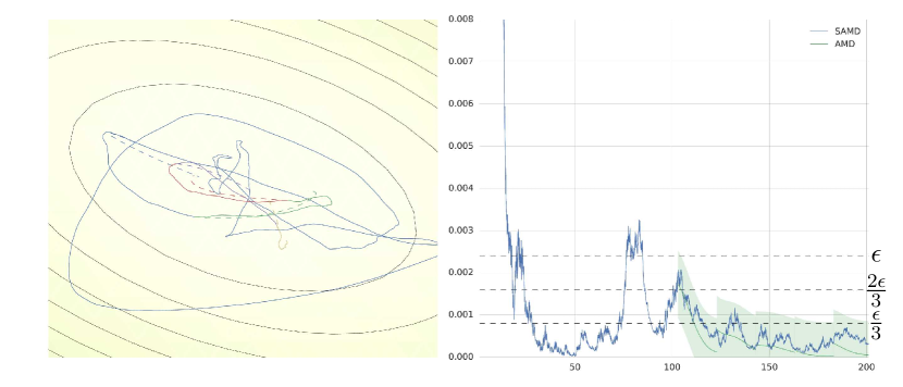
Figure 4: Illustration of the proof of TheoremΒ 1, with Ο΅=2.4 10βˆ’3italic-Ο΅superscript2.4103\epsilon=2.4\ 10^{-3}, and T0=20subscript𝑇020T_{0}=20. The right plot shows in blue the value of the energy function L¯​(X​(t),Z​(t))¯𝐿𝑋𝑑𝑍𝑑\bar{L}(X(t),Z(t)) along one sample trajectory (X​(t),Z​(t))𝑋𝑑𝑍𝑑(X(t),Z(t)) of the SAMD dynamics; and in green the energy function along solutions of the deterministic ODE {(xk​(t),zk​(t)),t∈[T2+k​T0,T2+(k+1)​T0]}subscriptπ‘₯π‘˜π‘‘subscriptπ‘§π‘˜π‘‘π‘‘subscript𝑇2π‘˜subscript𝑇0subscript𝑇2π‘˜1subscript𝑇0\{(x_{k}(t),z_{k}(t)),{t\in[T_{2}+kT_{0},T_{2}+(k+1)T_{0}]}\}, initialized at (X​(T2+k​T0),Z​(T2+k​T0))𝑋subscript𝑇2π‘˜subscript𝑇0𝑍subscript𝑇2π‘˜subscript𝑇0(X(T_{2}+kT_{0}),Z(T_{2}+kT_{0})). We also highlight a cylinder of radius Ο΅3italic-Ο΅3\frac{\epsilon}{3} centered at the deterministic energy. Note that for large enough times, the sample path of the stochastic dynamics remains within the cylinder. The dashed lines show the energy levels Ο΅3italic-Ο΅3\frac{\epsilon}{3}, 2​ϡ32italic-Ο΅3\frac{2\epsilon}{3}, and Ο΅italic-Ο΅\epsilon. Finally, the left plot visualizes these trajectories in the primal space (where we used a different color for each interval [T2+k​T0,T2+(k+1)​T0]subscript𝑇2π‘˜subscript𝑇0subscript𝑇2π‘˜1subscript𝑇0[T_{2}+kT_{0},T_{2}+(k+1)T_{0}]).

We are now ready to put together the different parts of the argument. Fix Ο΅>0italic-Ο΅0\epsilon>0.
By (ii), there exists T0subscript𝑇0T_{0} such that

L¯​(Ξ¦T0​(x),Ξ¦T0​(z))≀min⁑(Ο΅/3,L¯​(x,z)βˆ’Ο΅/3).¯𝐿subscriptΞ¦subscript𝑇0π‘₯subscriptΞ¦subscript𝑇0𝑧italic-Ο΅3¯𝐿π‘₯𝑧italic-Ο΅3\bar{L}(\Phi_{T_{0}}(x),\Phi_{T_{0}}(z))\leq\min(\epsilon/3,\bar{L}(x,z)-\epsilon/3). (23)

By (i) there exists T1subscript𝑇1T_{1} such that for tβ‰₯T1𝑑subscript𝑇1t\geq T_{1} and for all h∈[0,T0]β„Ž0subscript𝑇0h\in[0,T_{0}],

L¯​(X​(t+h),Z​(t+h))≀L¯​(Ξ¦h​(X​(t),Z​(t)))+Ο΅/3,Β―πΏπ‘‹π‘‘β„Žπ‘π‘‘β„ŽΒ―πΏsubscriptΞ¦β„Žπ‘‹π‘‘π‘π‘‘italic-Ο΅3\bar{L}(X(t+h),Z(t+h))\leq\bar{L}(\Phi_{h}(X(t),Z(t)))+\epsilon/3, (24)

By (iii), there exists T2β‰₯max⁑(T0,T1)subscript𝑇2subscript𝑇0subscript𝑇1T_{2}\geq\max(T_{0},T_{1}) such that (X​(T2),Z​(T2))∈VΟ΅/3𝑋subscript𝑇2𝑍subscript𝑇2subscript𝑉italic-Ο΅3(X(T_{2}),Z(T_{2}))\in V_{\epsilon/3}.

Now we show that the trajectory remains in VΟ΅subscript𝑉italic-Ο΅V_{\epsilon} for all tβ‰₯T2𝑑subscript𝑇2t\geq T_{2}. Indeed, by induction on kπ‘˜k, we have L¯​(X​(T2+k​T0),Z​(T2+k​T0))≀2​ϡ/3¯𝐿𝑋subscript𝑇2π‘˜subscript𝑇0𝑍subscript𝑇2π‘˜subscript𝑇02italic-Ο΅3\bar{L}(X(T_{2}+kT_{0}),Z(T_{2}+kT_{0}))\leq{2\epsilon/3} for all kβˆˆβ„•π‘˜β„•k\in\mathbb{N} (byΒ (23) andΒ (24)), then for all h∈[0,T0]β„Ž0subscript𝑇0h\in[0,T_{0}],

L¯​(X​(T2+k​T0+h),Z​(T2+k​T0+h))¯𝐿𝑋subscript𝑇2π‘˜subscript𝑇0β„Žπ‘subscript𝑇2π‘˜subscript𝑇0β„Ž\displaystyle\bar{L}(X(T_{2}+kT_{0}+h),Z(T_{2}+kT_{0}+h)) ≀L¯​(Ξ¦h​(X​(T2+k​T0),Z​(T2+k​T0)))+Ο΅/3absent¯𝐿subscriptΞ¦β„Žπ‘‹subscript𝑇2π‘˜subscript𝑇0𝑍subscript𝑇2π‘˜subscript𝑇0italic-Ο΅3\displaystyle\leq\bar{L}(\Phi_{h}(X(T_{2}+kT_{0}),Z(T_{2}+kT_{0})))+\epsilon/3
≀2​ϡ/3+Ο΅/3.absent2italic-Ο΅3italic-Ο΅3\displaystyle\leq 2\epsilon/3+\epsilon/3.

Since Ο΅italic-Ο΅\epsilon is arbitrary, this proves that for all Ο΅italic-Ο΅\epsilon, (X​(t),Z​(t))𝑋𝑑𝑍𝑑(X(t),Z(t)) remains in VΟ΅subscript𝑉italic-Ο΅V_{\epsilon} for t𝑑t large enough, a.s. But by definition of L¯¯𝐿\bar{L}, (x,z)∈VΟ΅π‘₯𝑧subscript𝑉italic-Ο΅(x,z)\in V_{\epsilon} implies that f​(x)βˆ’f​(x⋆)≀ϡ𝑓π‘₯𝑓superscriptπ‘₯⋆italic-Ο΅f(x)-f(x^{\star})\leq\epsilon, which proves that f​(X​(t))βˆ’f​(x⋆)𝑓𝑋𝑑𝑓superscriptπ‘₯⋆f(X(t))-f(x^{\star}) converges to 00. ∎

4.2 Convergence of expected function values

Next, we derive explicit bounds on function values.

Theorem 2.

Suppose that AssumptionsΒ 1 and 3 hold. Suppose that a=Ξ·/rπ‘Žπœ‚π‘Ÿa=\eta/r and Ξ·β‰₯rΛ™πœ‚Λ™π‘Ÿ\eta\geq\dot{r}. Let (X​(t),Z​(t))𝑋𝑑𝑍𝑑(X(t),Z(t)) be the unique continuous solution to SAMDΞ·,Ξ·/r,ssubscriptSAMDπœ‚πœ‚π‘Ÿπ‘ \operatorname{SAMD}_{\eta,\eta/r,s}. Then for all tβ‰₯t0𝑑subscript𝑑0t\geq t_{0},

𝔼​[f​(X​(t))]βˆ’f​(x⋆)≀L​(x0,z0,t0)+Οˆβ€‹(x⋆)​(s​(t)βˆ’s​(t0))+n​LΟˆβˆ—2β€‹βˆ«t0tΞ·2​(Ο„)β€‹Οƒβˆ—2​(Ο„)s​(Ο„)​𝑑τr​(t).𝔼delimited-[]𝑓𝑋𝑑𝑓superscriptπ‘₯⋆𝐿subscriptπ‘₯0subscript𝑧0subscript𝑑0πœ“superscriptπ‘₯⋆𝑠𝑑𝑠subscript𝑑0𝑛subscript𝐿superscriptπœ“2superscriptsubscriptsubscript𝑑0𝑑superscriptπœ‚2𝜏superscriptsubscript𝜎2πœπ‘ πœdifferential-dπœπ‘Ÿπ‘‘\displaystyle\mathbb{E}[f(X(t))]-f(x^{\star})\leq\frac{L(x_{0},z_{0},t_{0})+\psi(x^{\star})(s(t)-s(t_{0}))+\frac{nL_{\psi^{*}}}{2}\int_{t_{0}}^{t}\frac{\eta^{2}(\tau)\sigma_{*}^{2}(\tau)}{s(\tau)}d\tau}{r(t)}.
Proof.

Integrating the bound of LemmaΒ 2, and using the fact that (f​(X​(t))βˆ’f​(x⋆))​(rΛ™βˆ’Ξ·)≀0𝑓𝑋𝑑𝑓superscriptπ‘₯β‹†Λ™π‘Ÿπœ‚0(f(X(t))-f(x^{\star}))(\dot{r}-\eta)\leq 0 by assumption on Ξ·πœ‚\eta, we have

L​(X​(t),Z​(t),t)βˆ’L​(x0,z0,t0)β‰€Οˆβ€‹(x⋆)​(s​(t)βˆ’s​(t0))+n​LΟˆβˆ—2β€‹βˆ«t0tΞ·2​(Ο„)β€‹Οƒβˆ—2​(Ο„)s​(Ο„)​𝑑τ+∫t0t⟨V​(Ο„),d​B​(Ο„)⟩,𝐿𝑋𝑑𝑍𝑑𝑑𝐿subscriptπ‘₯0subscript𝑧0subscript𝑑0πœ“superscriptπ‘₯⋆𝑠𝑑𝑠subscript𝑑0𝑛subscript𝐿superscriptπœ“2superscriptsubscriptsubscript𝑑0𝑑superscriptπœ‚2𝜏superscriptsubscript𝜎2πœπ‘ πœdifferential-d𝜏superscriptsubscriptsubscript𝑑0π‘‘π‘‰πœπ‘‘π΅πœL(X(t),Z(t),t)-L(x_{0},z_{0},t_{0})\leq\psi(x^{\star})(s(t)-s(t_{0}))+\frac{nL_{\psi^{*}}}{2}\int_{t_{0}}^{t}\frac{\eta^{2}(\tau)\sigma_{*}^{2}(\tau)}{s(\tau)}d\tau+\int_{t_{0}}^{t}\left\langle V(\tau),dB(\tau)\right\rangle, (25)

Taking expectations, the last term vanishes since it is an ItΓ΄ martingale, and we conclude by observing that 𝔼​[f​(X​(t))]βˆ’f​(x⋆)≀𝔼​[L​(X​(t),Z​(t),t)]/r​(t)𝔼delimited-[]𝑓𝑋𝑑𝑓superscriptπ‘₯⋆𝔼delimited-[]πΏπ‘‹π‘‘π‘π‘‘π‘‘π‘Ÿπ‘‘\mathbb{E}[f(X(t))]-f(x^{\star})\leq\mathbb{E}[L(X(t),Z(t),t)]/r(t). ∎

To give a concrete example, suppose that Οƒβˆ—β€‹(t)=π’ͺ​(tΞ±Οƒ)subscriptπœŽπ‘‘π’ͺsuperscript𝑑subscriptπ›ΌπœŽ\sigma_{*}(t)=\mathcal{O}(t^{\alpha_{\sigma}}) is given, and let r​(t)=tΞ±rπ‘Ÿπ‘‘superscript𝑑subscriptπ›Όπ‘Ÿr(t)=t^{\alpha_{r}} and s​(t)=tΞ±s𝑠𝑑superscript𝑑subscript𝛼𝑠s(t)=t^{\alpha_{s}}, Ξ±r,Ξ±s>0subscriptπ›Όπ‘Ÿsubscript𝛼𝑠0\alpha_{r},\alpha_{s}>0. To simplify, we will take η​(t)=r˙​(t)=Ξ±r​tΞ±rβˆ’1πœ‚π‘‘Λ™π‘Ÿπ‘‘subscriptπ›Όπ‘Ÿsuperscript𝑑subscriptπ›Όπ‘Ÿ1\eta(t)=\dot{r}(t)=\alpha_{r}t^{\alpha_{r}-1}. Then the bound of TheoremΒ 2 shows that 𝔼​[f​(X​(t))]βˆ’f​(x⋆)=π’ͺ​(tΞ±sβˆ’Ξ±r+tΞ±r+2β€‹Ξ±Οƒβˆ’Ξ±sβˆ’1)𝔼delimited-[]𝑓𝑋𝑑𝑓superscriptπ‘₯⋆π’ͺsuperscript𝑑subscript𝛼𝑠subscriptπ›Όπ‘Ÿsuperscript𝑑subscriptπ›Όπ‘Ÿ2subscriptπ›ΌπœŽsubscript𝛼𝑠1\mathbb{E}[f(X(t))]-f(x^{\star})=\mathcal{O}(t^{\alpha_{s}-\alpha_{r}}+t^{\alpha_{r}+2\alpha_{\sigma}-\alpha_{s}-1}). To minimize the asymptotic rate, we can choose Ξ±sβˆ’Ξ±r=Ξ±r+2β€‹Ξ±Οƒβˆ’Ξ±sβˆ’1subscript𝛼𝑠subscriptπ›Όπ‘Ÿsubscriptπ›Όπ‘Ÿ2subscriptπ›ΌπœŽsubscript𝛼𝑠1\alpha_{s}-\alpha_{r}=\alpha_{r}+2\alpha_{\sigma}-\alpha_{s}-1, i.e. Ξ±r+Ξ±Οƒβˆ’Ξ±sβˆ’12=0subscriptπ›Όπ‘Ÿsubscriptπ›ΌπœŽsubscript𝛼𝑠120\alpha_{r}+\alpha_{\sigma}-\alpha_{s}-\frac{1}{2}=0 (it is always possible to find such Ξ±r,Ξ±s>0subscriptπ›Όπ‘Ÿsubscript𝛼𝑠0\alpha_{r},\alpha_{s}>0), and the resulting rate is π’ͺ​(tΞ±Οƒβˆ’12)π’ͺsuperscript𝑑subscriptπ›ΌπœŽ12\mathcal{O}(t^{\alpha_{\sigma}-\frac{1}{2}}).

Corollary 2.

Suppose that AssumptionsΒ 1 and 3 hold. Suppose that Οƒβˆ—β€‹(t)=π’ͺ​(tΞ±Οƒ)subscriptπœŽπ‘‘π’ͺsuperscript𝑑subscriptπ›ΌπœŽ\sigma_{*}(t)=\mathcal{O}(t^{\alpha_{\sigma}}), Ξ±Οƒ<12subscriptπ›ΌπœŽ12\alpha_{\sigma}<\frac{1}{2}. Consider SAMDΞ·,Ξ·/r,ssubscriptSAMDπœ‚πœ‚π‘Ÿπ‘ \operatorname{SAMD}_{\eta,\eta/r,s} dynamics with r​(t)=tΞ±rπ‘Ÿπ‘‘superscript𝑑subscriptπ›Όπ‘Ÿr(t)=t^{\alpha_{r}}, η​(t)=r˙​(t)=Ξ±r​tΞ±rβˆ’1πœ‚π‘‘Λ™π‘Ÿπ‘‘subscriptπ›Όπ‘Ÿsuperscript𝑑subscriptπ›Όπ‘Ÿ1\eta(t)=\dot{r}(t)=\alpha_{r}t^{\alpha_{r}-1}, and s​(t)=tΞ±s𝑠𝑑superscript𝑑subscript𝛼𝑠s(t)=t^{\alpha_{s}}, and suppose that

Ξ±r=Ξ±sβˆ’Ξ±Οƒ+12subscriptπ›Όπ‘Ÿsubscript𝛼𝑠subscriptπ›ΌπœŽ12\alpha_{r}=\alpha_{s}-\alpha_{\sigma}+\frac{1}{2}

Then

𝔼​[f​(X​(t))]βˆ’f​(x⋆)=π’ͺ​(tΞ±Οƒβˆ’12)𝔼delimited-[]𝑓𝑋𝑑𝑓superscriptπ‘₯⋆π’ͺsuperscript𝑑subscriptπ›ΌπœŽ12\displaystyle\mathbb{E}[f(X(t))]-f(x^{\star})=\mathcal{O}(t^{\alpha_{\sigma}-\frac{1}{2}}) as tβ†’βˆžβ†’π‘‘t\to\infty.

In particular, CorollaryΒ 2 indicates that it is possible to obtain convergence rates faster than π’ͺ​(1t)π’ͺ1𝑑\mathcal{O}(\frac{1}{t}) if the gradient noise decays fast enough.

Remark 4.

This result is reminiscent of the results ofΒ Schmidt etΒ al. (2011), who studied the convergence rates of inexact accelerated methods (in discrete time), in which the gradient is evaluated at step kπ‘˜k up to an error term eksubscriptπ‘’π‘˜e_{k}. They show that the optimality gap (function values in expectation) at step kπ‘˜k is π’ͺ​(βˆ‘ΞΊ=1kκ​eΞΊk2)π’ͺsuperscriptsubscriptπœ…1π‘˜πœ…subscriptπ‘’πœ…superscriptπ‘˜2\mathcal{O}(\frac{\sum_{\kappa=1}^{k}\kappa e_{\kappa}}{k^{2}}). Although the settings are different (their analysis is done for deterministic, discrete methods), the results are similar. In particular, when eksubscriptπ‘’π‘˜e_{k} decays as π’ͺ​(kΞ±Οƒ)π’ͺsuperscriptπ‘˜subscriptπ›ΌπœŽ\mathcal{O}(k^{\alpha_{\sigma}}), the resulting convergence rate of Nesterov’s accelerated method is π’ͺ​(βˆ‘ΞΊ=1kκ​κασk2)=π’ͺ​(kΞ±Οƒ)π’ͺsuperscriptsubscriptπœ…1π‘˜πœ…superscriptπœ…subscriptπ›ΌπœŽsuperscriptπ‘˜2π’ͺsuperscriptπ‘˜subscriptπ›ΌπœŽ\mathcal{O}(\frac{\sum_{\kappa=1}^{k}\kappa\kappa^{\alpha_{\sigma}}}{k^{2}})=\mathcal{O}(k^{\alpha_{\sigma}}), which appears slower than the π’ͺ​(tΞ±Οƒβˆ’12)π’ͺsuperscript𝑑subscriptπ›ΌπœŽ12\mathcal{O}(t^{\alpha_{\sigma}}-\frac{1}{2}) of CorollaryΒ 2. This is due to the fact that Nesterov’s method corresponds to r​(t)=Ξ˜β€‹(t2),s​(t)=Ξ˜β€‹(1)formulae-sequenceπ‘Ÿπ‘‘Ξ˜superscript𝑑2π‘ π‘‘Ξ˜1r(t)=\Theta(t^{2}),s(t)=\Theta(1) (see AppendixΒ A), which is not the optimal choice of decay rate according to the corollary.

Remark 5 (Dependence on the dimension).

Note that we can potentially scale the rates η​(t),r​(t)πœ‚π‘‘π‘Ÿπ‘‘\eta(t),r(t) in order to improve the dependence of the boundΒ (25) on the dimension n𝑛n. Note that the second term in the bound of TheoremΒ 2 involves the quantity Οˆβ€‹(x⋆)πœ“superscriptπ‘₯⋆\psi(x^{\star}), which can be bounded by supxβˆˆπ’³Οˆβ€‹(x)subscriptsupremumπ‘₯π’³πœ“π‘₯\sup_{x\in\mathcal{X}}\psi(x) when 𝒳𝒳\mathcal{X} is compact, and this supremum is often a non-decreasing function of n𝑛n (for example, in the case of the negative entropy on the simplex, we have that supxβˆˆπ’³Οˆβ€‹(x)=supxβˆˆπ’³βˆ‘i=1nxi​ln⁑xi=log⁑nsubscriptsupremumπ‘₯π’³πœ“π‘₯subscriptsupremumπ‘₯𝒳superscriptsubscript𝑖1𝑛subscriptπ‘₯𝑖subscriptπ‘₯𝑖𝑛\sup_{x\in\mathcal{X}}\psi(x)=\sup_{x\in\mathcal{X}}\sum_{i=1}^{n}x_{i}\ln x_{i}=\log n). Thus let us denote the supremum by M​(n)𝑀𝑛M(n), and assume that Ξ·,r,aπœ‚π‘Ÿπ‘Ž\eta,r,a are given and satisfy the conditions of TheoremΒ 2. Define the rescaled weights η¯​(t)=Ξ·0​(n)​η​(t)Β―πœ‚π‘‘subscriptπœ‚0π‘›πœ‚π‘‘\bar{\eta}(t)=\eta_{0}(n)\eta(t), r¯​(t)=Ξ·0​(n)​r​(t)Β―π‘Ÿπ‘‘subscriptπœ‚0π‘›π‘Ÿπ‘‘\bar{r}(t)=\eta_{0}(n)r(t) (note that we scale both Ξ·πœ‚\eta and rπ‘Ÿr so that the condition Ξ·β‰₯rΛ™πœ‚Λ™π‘Ÿ\eta\geq\dot{r} still holds, and we do not need to scale aπ‘Ža since a=Ξ·/r=Ξ·Β―/rΒ―π‘Žπœ‚π‘ŸΒ―πœ‚Β―π‘Ÿa=\eta/r=\bar{\eta}/\bar{r}). Then applying TheoremΒ 2 to SAMDΞ·Β―,Ξ·Β―/rΒ―,ssubscriptSAMDΒ―πœ‚Β―πœ‚Β―π‘Ÿπ‘ \operatorname{SAMD}_{\bar{\eta},\bar{\eta}/\bar{r},s} gives us

𝔼𝔼\displaystyle\mathbb{E} [f​(X​(t))]βˆ’f​(x⋆)≀L​(x0,z0,t0)+M​(n)​s​(t)+n​LΟˆβˆ—β€‹Ξ·02​(n)2β€‹βˆ«t0tΞ·2​(Ο„)β€‹Οƒβˆ—2​(Ο„)s​(Ο„)​𝑑τη0​(n)​r​(t)delimited-[]𝑓𝑋𝑑𝑓superscriptπ‘₯⋆𝐿subscriptπ‘₯0subscript𝑧0subscript𝑑0𝑀𝑛𝑠𝑑𝑛subscript𝐿superscriptπœ“superscriptsubscriptπœ‚02𝑛2superscriptsubscriptsubscript𝑑0𝑑superscriptπœ‚2𝜏superscriptsubscript𝜎2πœπ‘ πœdifferential-d𝜏subscriptπœ‚0π‘›π‘Ÿπ‘‘\displaystyle[f(X(t))]-f(x^{\star})\leq\frac{L(x_{0},z_{0},t_{0})+M(n)s(t)+\frac{nL_{\psi^{*}}\eta_{0}^{2}(n)}{2}\int_{t_{0}}^{t}\frac{\eta^{2}(\tau)\sigma_{*}^{2}(\tau)}{s(\tau)}d\tau}{\eta_{0}(n)r(t)}

where L​(x0,z0,t0)=Ξ·0​(n)​r​(t0)​(f​(x0)βˆ’f​(x⋆))+s​(t0)​DΟˆβˆ—β€‹(z0,z⋆)𝐿subscriptπ‘₯0subscript𝑧0subscript𝑑0subscriptπœ‚0π‘›π‘Ÿsubscript𝑑0𝑓subscriptπ‘₯0𝑓superscriptπ‘₯⋆𝑠subscript𝑑0subscript𝐷superscriptπœ“subscript𝑧0superscript𝑧⋆L(x_{0},z_{0},t_{0})=\eta_{0}(n)r(t_{0})(f(x_{0})-f(x^{\star}))+s(t_{0})D_{\psi^{*}}(z_{0},z^{\star}) and is dominated by the other terms (assuming that DΟˆβˆ—β€‹(z0,z⋆)=π’ͺ​(M​(n))subscript𝐷superscriptπœ“subscript𝑧0superscript𝑧⋆π’ͺ𝑀𝑛D_{\psi^{*}}(z_{0},z^{\star})=\mathcal{O}(M(n)) to simplify). Thus we have, asymptotically as nβ†’βˆžβ†’π‘›n\to\infty,

𝔼𝔼\displaystyle\mathbb{E} [f​(X​(t))]βˆ’f​(x⋆)=π’ͺ​(M​(n)Ξ·0​(n)+n​η0​(n))delimited-[]𝑓𝑋𝑑𝑓superscriptπ‘₯⋆π’ͺ𝑀𝑛subscriptπœ‚0𝑛𝑛subscriptπœ‚0𝑛\displaystyle[f(X(t))]-f(x^{\star})=\mathcal{O}\left(\frac{M(n)}{\eta_{0}(n)}+n\eta_{0}(n)\right)

and choosing Ξ·0​(n)=M​(n)nsubscriptπœ‚0𝑛𝑀𝑛𝑛\eta_{0}(n)=\sqrt{\frac{M(n)}{n}} minimizes the asymptotic growth rate of the bound, resulting in

𝔼​[f​(X​(t))]βˆ’f​(x⋆)=π’ͺ​(n​M​(n))𝔼delimited-[]𝑓𝑋𝑑𝑓superscriptπ‘₯⋆π’ͺ𝑛𝑀𝑛\displaystyle\mathbb{E}[f(X(t))]-f(x^{\star})=\mathcal{O}(\sqrt{nM(n)}) asΒ nβ†’βˆž.asΒ nβ†’βˆž\displaystyle\text{as $n\to\infty$}.

We now illustrate the asymptotic rates of TheoremΒ 2, and the optimal choice of primal and dual rates given in CorollaryΒ 2 on the simplex-constrained sum-exponential example of SectionΒ 3.1. We simulate solution trajectories of SAMDΞ·,Ξ·/r,ssubscriptSAMDπœ‚πœ‚π‘Ÿπ‘ \operatorname{SAMD}_{\eta,\eta/r,s} under different noise regimes, by taking Οƒβˆ—β€‹(t)=10βˆ’1​tΞ±ΟƒsuperscriptπœŽπ‘‘superscript101superscript𝑑subscriptπ›ΌπœŽ\sigma^{*}(t)=10^{-1}t^{\alpha_{\sigma}} for different values of Ξ±Οƒsubscriptπ›ΌπœŽ\alpha_{\sigma}, and for different configurations of rates r​(t)=tΞ±rπ‘Ÿπ‘‘superscript𝑑subscriptπ›Όπ‘Ÿr(t)=t^{\alpha_{r}}, s​(t)=tΞ±s𝑠𝑑superscript𝑑subscript𝛼𝑠s(t)=t^{\alpha_{s}}. To simplify, we took η​(t)=r˙​(t)πœ‚π‘‘Λ™π‘Ÿπ‘‘\eta(t)=\dot{r}(t). We plot the mean and standard deviation over 100100100 simulations. In particular, we seek to verify whether the optimal decay rates are given by Ξ±r=Ξ±sβˆ’Ξ±Οƒ+12subscriptπ›Όπ‘Ÿsubscript𝛼𝑠subscriptπ›ΌπœŽ12\alpha_{r}=\alpha_{s}-\alpha_{\sigma}+\frac{1}{2}, as predicted by CorollaryΒ 2. The results are given in FigureΒ 4.

For each choice of Ξ±rsubscriptπ›Όπ‘Ÿ\alpha_{r}, we evaluate the decay rate of expected function values (using the empirical mean over 100100100 runs). The optimal decay rate Ξ±rsubscriptπ›Όπ‘Ÿ\alpha_{r}, and the resulting decay of function values, seem consistent with the predictions of the Corollary when Οƒβˆ—β€‹(t)subscriptπœŽπ‘‘\sigma_{*}(t) is non-decreasing (i.e. Ξ±Οƒβ‰₯0subscriptπ›ΌπœŽ0\alpha_{\sigma}\geq 0). However, for decreasing Οƒβˆ—β€‹(t)subscriptπœŽπ‘‘\sigma_{*}(t) (i.e. in the vanishing noise regime), the estimates of the Corollary seem to be conservative. The optimal rate Ξ±rsubscriptπ›Όπ‘Ÿ\alpha_{r} which we observed was slower than predicted, and the resulting convergence rate was faster, see FigureΒ 4 for examples. It is also interesting to observe the effect of varying the averaging rates on the trajectory: a faster decay of the sensitivity 1/s​(t)1𝑠𝑑1/s(t), or similarly a faster decay of the dual weight η​(t)πœ‚π‘‘\eta(t), results in a decrease of the period of oscillations of the accelerated dynamics.

[Uncaptioned image]
[Uncaptioned image]
[Uncaptioned image]
[Uncaptioned image]
[Uncaptioned image]
[Uncaptioned image]
Refer to caption
Refer to caption
Figure 4: Mean and standard deviation of function values along solution trajectories of SAMDrΛ™,rΛ™/r,ssubscriptSAMDΛ™π‘ŸΛ™π‘Ÿπ‘Ÿπ‘ \operatorname{SAMD}_{\dot{r},\dot{r}/r,s}, for different configurations of rates r​(t)=tΞ±r,s​(t)=tΞ±sformulae-sequenceπ‘Ÿπ‘‘superscript𝑑subscriptπ›Όπ‘Ÿπ‘ π‘‘superscript𝑑subscript𝛼𝑠r(t)=t^{\alpha_{r}},s(t)=t^{\alpha_{s}}, and different noise regimes Οƒβˆ—β€‹(t)=10βˆ’1​tΞ±ΟƒsubscriptπœŽπ‘‘superscript101superscript𝑑subscriptπ›ΌπœŽ\sigma_{*}(t)=10^{-1}t^{\alpha_{\sigma}}. Each row correspond to a different noise regime (Ξ±Οƒ=.2subscriptπ›ΌπœŽ.2\alpha_{\sigma}=.2 for the first row, 00 for the second, βˆ’.5.5-.5 for the third, and βˆ’11-1 for the last), and each column corresponds to a different decay rate of the sensitivity (Ξ±s=.5subscript𝛼𝑠.5\alpha_{s}=.5 for the first column, 111 for the second). Each figure contains multiple plots corresponding to different Ξ±rsubscriptπ›Όπ‘Ÿ\alpha_{r}. For the first two rows, Ξ±r=Ξ±sβˆ’Ξ±Οƒ+.5subscriptπ›Όπ‘Ÿsubscript𝛼𝑠subscriptπ›ΌπœŽ.5\alpha_{r}=\alpha_{s}-\alpha_{\sigma}+.5 gives the optimal rate, as predicted by CorollaryΒ 2. However, for the last two rows, the best decay rate is achieved by Ξ±rsubscriptπ›Όπ‘Ÿ\alpha_{r} is lower, namely Ξ±r=Ξ±sβˆ’Ξ±Οƒ+.3subscriptπ›Όπ‘Ÿsubscript𝛼𝑠subscriptπ›ΌπœŽ.3\alpha_{r}=\alpha_{s}-\alpha_{\sigma}+.3 for the third row, and Ξ±r=Ξ±sβˆ’Ξ±Οƒ+.1subscriptπ›Όπ‘Ÿsubscript𝛼𝑠subscriptπ›ΌπœŽ.1\alpha_{r}=\alpha_{s}-\alpha_{\sigma}+.1 for the last.

4.3 Almost sure asymptotic rates

Finally, we give an estimate of the asymptotic convergence rate along solution trajectories, under the additional compactness assumption (to be able to bound the martingale term, using LemmaΒ 3).

Theorem 3.

Suppose that AssumptionsΒ 1, 2 and 3 hold, and suppose that a=Ξ·/rπ‘Žπœ‚π‘Ÿa=\eta/r and Ξ·β‰₯rΛ™πœ‚Λ™π‘Ÿ\eta\geq\dot{r}. Let (X​(t),Z​(t))𝑋𝑑𝑍𝑑(X(t),Z(t)) be the unique continuous solution to SAMDΞ·,Ξ·/r,ssubscriptSAMDπœ‚πœ‚π‘Ÿπ‘ \operatorname{SAMD}_{\eta,\eta/r,s}. Then

f​(X​(t))βˆ’f​(x⋆)=π’ͺ​(s​(t)+nβ€‹βˆ«t0tΞ·2​(Ο„)β€‹Οƒβˆ—2​(Ο„)s​(Ο„)+b​(t)​log⁑log⁑b​(t)r​(t))𝑓𝑋𝑑𝑓superscriptπ‘₯⋆π’ͺ𝑠𝑑𝑛superscriptsubscriptsubscript𝑑0𝑑superscriptπœ‚2𝜏superscriptsubscript𝜎2πœπ‘ πœπ‘π‘‘π‘π‘‘π‘Ÿπ‘‘\displaystyle f(X(t))-f(x^{\star})=\mathcal{O}\left(\frac{s(t)+n\int_{t_{0}}^{t}\frac{\eta^{2}(\tau)\sigma_{*}^{2}(\tau)}{s(\tau)}+\sqrt{b(t)\log\log b(t)}}{r(t)}\right) a.s. as tβ†’βˆžβ†’π‘‘t\to\infty,

where b​(t)=∫t0tΞ·2​(Ο„)β€‹Οƒβˆ—2​(Ο„)​𝑑τ𝑏𝑑superscriptsubscriptsubscript𝑑0𝑑superscriptπœ‚2𝜏superscriptsubscript𝜎2𝜏differential-d𝜏b(t)=\int_{t_{0}}^{t}\eta^{2}(\tau)\sigma_{*}^{2}(\tau)d\tau.

Proof.

Integrating the bound of LemmaΒ 2 once again, we get inequalityΒ (25), where we can bound the ItΓ΄ martingale term ∫t0t⟨V​(Ο„),d​B​(Ο„)⟩superscriptsubscriptsubscript𝑑0π‘‘π‘‰πœπ‘‘π΅πœ\int_{t_{0}}^{t}\left\langle V(\tau),dB(\tau)\right\rangle using LemmaΒ 3, since 𝒳𝒳\mathcal{X} is now assumed compact. This concludes the proof. ∎

Comparing the last bound to that of TheoremΒ 2, we have the additional b​(t)​log⁑log⁑b​(t)r​(t)π‘π‘‘π‘π‘‘π‘Ÿπ‘‘\frac{\sqrt{b(t)\log\log b(t)}}{r(t)} term due to the envelope of the martingale term. This results in a slower a.s. convergence rate. To give a concrete example, suppose again that Οƒβˆ—β€‹(t)=π’ͺ​(tσα)subscriptπœŽπ‘‘π’ͺsubscriptsuperscriptπ‘‘π›ΌπœŽ\sigma_{*}(t)=\mathcal{O}(t^{\alpha}_{\sigma}), and that r​(t)=tΞ²π‘Ÿπ‘‘superscript𝑑𝛽r(t)=t^{\beta} and η​(t)=r˙​(t)=β​tΞ²βˆ’1πœ‚π‘‘Λ™π‘Ÿπ‘‘π›½superscript𝑑𝛽1\eta(t)=\dot{r}(t)=\beta t^{\beta-1} to simplify. Then b​(t)=∫t0tΞ·2​(Ο„)β€‹Οƒβˆ—2​(Ο„)​𝑑τ=π’ͺ​(t2​β+2β€‹Ξ±Οƒβˆ’1)𝑏𝑑superscriptsubscriptsubscript𝑑0𝑑superscriptπœ‚2𝜏superscriptsubscript𝜎2𝜏differential-d𝜏π’ͺsuperscript𝑑2𝛽2subscriptπ›ΌπœŽ1b(t)=\int_{t_{0}}^{t}\eta^{2}(\tau)\sigma_{*}^{2}(\tau)d\tau=\mathcal{O}(t^{2\beta+2\alpha_{\sigma}-1}), and the martingale term becomes π’ͺ​(b​(t)​log⁑log⁑b​(t)/r​(t))=π’ͺ​(tΞ±Οƒβˆ’12​log⁑log⁑t)π’ͺπ‘π‘‘π‘π‘‘π‘Ÿπ‘‘π’ͺsuperscript𝑑subscriptπ›ΌπœŽ12𝑑\mathcal{O}(\sqrt{b(t)\log\log b(t)}/r(t))=\mathcal{O}(t^{\alpha_{\sigma}-\frac{1}{2}}\sqrt{\log\log t}). Remarkably, the convergence rate of sample trajectories is, up to a log⁑log⁑t𝑑\sqrt{\log\log t} factor, the same as the convergence rate in expectation.

Corollary 3.

Suppose that AssumptionsΒ 1, 2 and 3 hold, and suppose that Οƒβˆ—β€‹(t)=π’ͺ​(tΞ±Οƒ)subscriptπœŽπ‘‘π’ͺsuperscript𝑑subscriptπ›ΌπœŽ\sigma_{*}(t)=\mathcal{O}(t^{\alpha_{\sigma}}), Ξ±Οƒ<12subscriptπ›ΌπœŽ12\alpha_{\sigma}<\frac{1}{2}. Consider SAMDΞ·,Ξ·/r,ssubscriptSAMDπœ‚πœ‚π‘Ÿπ‘ \operatorname{SAMD}_{\eta,\eta/r,s} dynamics with r​(t)=tΞ±rπ‘Ÿπ‘‘superscript𝑑subscriptπ›Όπ‘Ÿr(t)=t^{\alpha_{r}}, η​(t)=r˙​(t)=Ξ±r​tΞ±rβˆ’1πœ‚π‘‘Λ™π‘Ÿπ‘‘subscriptπ›Όπ‘Ÿsuperscript𝑑subscriptπ›Όπ‘Ÿ1\eta(t)=\dot{r}(t)=\alpha_{r}t^{\alpha_{r}-1}, and s​(t)=tΞ±s𝑠𝑑superscript𝑑subscript𝛼𝑠s(t)=t^{\alpha_{s}}, and suppose that

Ξ±r=Ξ±sβˆ’Ξ±Οƒ+12.subscriptπ›Όπ‘Ÿsubscript𝛼𝑠subscriptπ›ΌπœŽ12\alpha_{r}=\alpha_{s}-\alpha_{\sigma}+\frac{1}{2}.

Then

f​(X​(t))βˆ’f​(x⋆)=π’ͺ​(tΞ±βˆ’12​log⁑log⁑t)𝑓𝑋𝑑𝑓superscriptπ‘₯⋆π’ͺsuperscript𝑑𝛼12𝑑\displaystyle f(X(t))-f(x^{\star})=\mathcal{O}(t^{\alpha-\frac{1}{2}}\sqrt{\log\log t}) a.s. as tβ†’βˆžβ†’π‘‘t\to\infty.

5 Numerical examples

In this section, we give additional numerical examples to illustrate the differences between SMDSMD\operatorname{SMD} and SAMDSAMD\operatorname{SAMD} dynamics. In order to compare the performance of the two methods, we derive, in AppendixΒ B, the convergence rates of (non-accelerated) stochastic mirror descent, in particular when Οƒβˆ—β€‹(t)subscriptπœŽπ‘‘\sigma_{*}(t) is asymptotically vanishing. CorollaryΒ 4 shows that when Οƒβˆ—β€‹(t)=π’ͺ​(tΞ±Οƒ)subscriptπœŽπ‘‘π’ͺsuperscript𝑑subscriptπ›ΌπœŽ\sigma_{*}(t)=\mathcal{O}(t^{\alpha_{\sigma}}), SMDSMD\operatorname{SMD} with inverse sensitivity rate s​(t)=tmax⁑(0,Ξ±Οƒ+12)𝑠𝑑superscript𝑑0subscriptπ›ΌπœŽ12s(t)=t^{\max(0,\alpha_{\sigma}+\frac{1}{2})} guarantees convergence of expected function values at the rate π’ͺ​(tmax⁑(Ξ±Οƒβˆ’12,1))π’ͺsuperscript𝑑subscriptπ›ΌπœŽ121\mathcal{O}(t^{\max(\alpha_{\sigma}-\frac{1}{2},1)}). So theoretically, when Ξ±Οƒβˆˆ[βˆ’12,12)subscriptπ›ΌπœŽ1212\alpha_{\sigma}\in[-\frac{1}{2},\frac{1}{2}), both methods are able to achieve the same asymptotic rates. However in practice, the accelerated dynamics exhibit desirable properties that we attempt to illustrate.

We consider again the simplex-constrained example of SectionΒ 3.1, so that we can visualize the trajectories and provide intuition. The objective function is given by the sum-exp function

f1​(x)=βˆ‘i=1ke⟨ci,x⟩,subscript𝑓1π‘₯superscriptsubscript𝑖1π‘˜superscript𝑒subscript𝑐𝑖π‘₯f_{1}(x)=\sum_{i=1}^{k}e^{\left\langle c_{i},x\right\rangle},

and in order to illustrate the non-strongly convex case, we also consider a simple convex quadratic of rank 111, given by

f2​(x)=12β€‹βŸ¨x,c⟩2=12​xT​c​cT​x.subscript𝑓2π‘₯12superscriptπ‘₯𝑐212superscriptπ‘₯𝑇𝑐superscript𝑐𝑇π‘₯f_{2}(x)=\frac{1}{2}\left\langle x,c\right\rangle^{2}=\frac{1}{2}x^{T}cc^{T}x.

The results are given in FigureΒ 5 andΒ 6, respectively. Qualitatively, SAMDSAMD\operatorname{SAMD} appears to exhibit smoother trajectories and a lower variance of the function values. Due to the oscillations of the accelerated dynamics, SAMDSAMD\operatorname{SAMD} initially makes slower progress (observe how SMDSMD\operatorname{SMD} trajectories make very fast progress in the initial steps), but makes faster progress in later iterations. A similar behavior is typical in the deterministic counterpart of the dynamics: accelerated mirror descent typically exhibits slower progress initially compared to non-accelerated mirror descent, but eventually makes faster progress.

Another difference which we observed in our numerical experiments is that the SAMDSAMD\operatorname{SAMD} dynamics seems more robust to much larger discretization step sizes (where we used a simple, constant-step discretization). Thus, even when SMDSMD\operatorname{SMD} theoretically achieves the same asymptotic rates of convergences as SAMDSAMD\operatorname{SAMD} (this is the case when Οƒβˆ—β€‹(t)=Ξ˜β€‹(tΞ±Οƒ)subscriptπœŽπ‘‘Ξ˜superscript𝑑subscriptπ›ΌπœŽ\sigma_{*}(t)=\Theta(t^{\alpha_{\sigma}}) with Ξ±Οƒβˆˆ[βˆ’12,12)subscriptπ›ΌπœŽ1212\alpha_{\sigma}\in[-\frac{1}{2},\frac{1}{2}), according to CorollaryΒ 2 and CorollaryΒ 4), SAMDSAMD\operatorname{SAMD} can, in practice, reach a target accuracy in fewer iterations.

In order to further illustrate the effect of the magnitude of the noise, we generate, in FigureΒ 7, different trajectories corresponding to SMDSMD\operatorname{SMD} and SAMDSAMD\operatorname{SAMD} dynamics, with a constant noise covariance given by Οƒβˆ—β€‹(t)β‰‘Οƒβˆ—subscriptπœŽπ‘‘subscript𝜎\sigma_{*}(t)\equiv\sigma_{*}. It is interesting to observe that for SAMDSAMD\operatorname{SAMD}, the magnitude of the noise seems to affect the amplitude of the oscillations, but not their period (the amplitude becomes smaller as the magnitude of the noise increases).
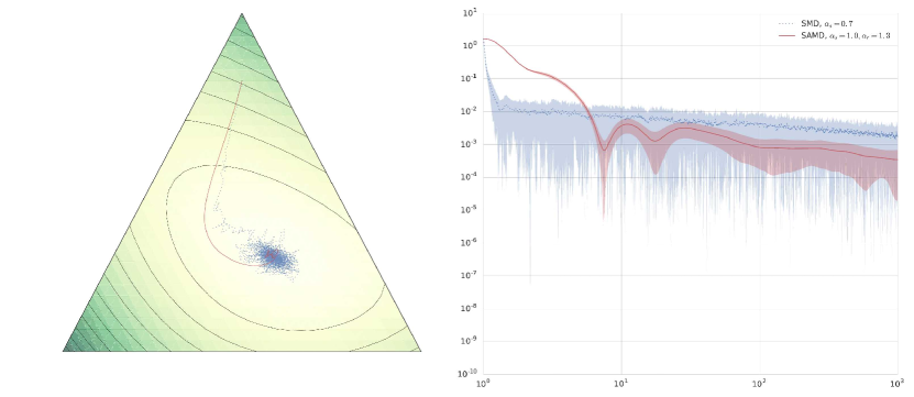
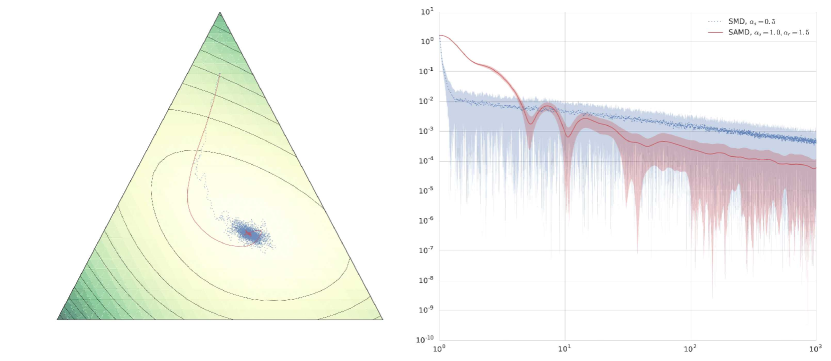
Refer to caption
Refer to caption
Refer to caption
Figure 5: Function values f1​(X​(t))βˆ’f1​(x⋆)subscript𝑓1𝑋𝑑subscript𝑓1superscriptπ‘₯⋆f_{1}(X(t))-f_{1}(x^{\star}), along solution trajectories X​(t)𝑋𝑑X(t) of SMDSMD\operatorname{SMD} and SAMDSAMD\operatorname{SAMD}, for different noise regimes Οƒβˆ—β€‹(t)=10βˆ’1​tΞ±ΟƒsubscriptπœŽπ‘‘superscript101superscript𝑑subscriptπ›ΌπœŽ\sigma_{*}(t)=10^{-1}t^{\alpha_{\sigma}}: Ξ±Οƒ=.2subscriptπ›ΌπœŽ.2\alpha_{\sigma}=.2 for the top figure, Ξ±Οƒ=0subscriptπ›ΌπœŽ0\alpha_{\sigma}=0 for the middle figure, and Ξ±Οƒ=βˆ’12subscriptπ›ΌπœŽ12\alpha_{\sigma}=-\frac{1}{2} for the bottom figure. The dynamics are configured according to the optimal rates of CorollaryΒ 2 and CorollaryΒ 4, i.e. Ξ±s=max⁑(0,Ξ±Οƒ+12)subscript𝛼𝑠0subscriptπ›ΌπœŽ12\alpha_{s}=\max(0,\alpha_{\sigma}+\frac{1}{2}) for SMDSMD\operatorname{SMD}, and Ξ±r=Ξ±sβˆ’Ξ±Οƒ+12subscriptπ›Όπ‘Ÿsubscript𝛼𝑠subscriptπ›ΌπœŽ12\alpha_{r}=\alpha_{s}-\alpha_{\sigma}+\frac{1}{2} for SAMDSAMD\operatorname{SAMD}.
Refer to caption
Refer to caption
Refer to caption
Figure 6: Function values f2​(X​(t))βˆ’f2​(x⋆)subscript𝑓2𝑋𝑑subscript𝑓2superscriptπ‘₯⋆f_{2}(X(t))-f_{2}(x^{\star}), along solution trajectories X​(t)𝑋𝑑X(t) of SMDSMD\operatorname{SMD} and SAMDSAMD\operatorname{SAMD}, for different noise regimes Οƒβˆ—β€‹(t)=10βˆ’1​tΞ±ΟƒsubscriptπœŽπ‘‘superscript101superscript𝑑subscriptπ›ΌπœŽ\sigma_{*}(t)=10^{-1}t^{\alpha_{\sigma}}.
Refer to caption
Refer to caption
Figure 7: Solution trajectories of SMDSMD\operatorname{SMD} (top) and SAMDSAMD\operatorname{SAMD} (bottom) dynamics for different values of noise covariance Οƒβˆ—subscript𝜎\sigma_{*}.

6 Discussion

Starting from the averaging formulation of accelerated mirror descent in continuous-time, and motivated by stochastic optimization, we formulated a stochastic variant by adding a noise process to the gradient, and studied the resulting SDE. We discussed the role played by each parameter: the dual learning rate η​(t)πœ‚π‘‘\eta(t), the inverse sensitivity parameter s​(t)𝑠𝑑s(t), and the noise covariation bound Οƒβˆ—β€‹(t)subscriptπœŽπ‘‘\sigma_{*}(t). In particular, we showed how the asymptotic bounds on Οƒβˆ—β€‹(t)subscriptπœŽπ‘‘\sigma_{*}(t) affect the choice of η​(t),s​(t)πœ‚π‘‘π‘ π‘‘\eta(t),s(t).

Our results show that in the persistent noise regime, thanks to averaging, it is possible to guarantee a.s. convergence, remarkably even when Οƒβˆ—β€‹(t)subscriptπœŽπ‘‘\sigma_{*}(t) is increasing (as long as Οƒβˆ—β€‹(t)=π’ͺ​(t)subscriptπœŽπ‘‘π’ͺ𝑑\sigma_{*}(t)=\mathcal{O}(\sqrt{t})). In the vanishing noise regime, the appropriate choice of η​(t),s​(t)πœ‚π‘‘π‘ π‘‘\eta(t),s(t) leads to improved convergence rates, e.g. to π’ͺ​(tΞ±Οƒβˆ’12)π’ͺsuperscript𝑑subscriptπ›ΌπœŽ12\mathcal{O}(t^{\alpha_{\sigma}-\frac{1}{2}}) in expectation and π’ͺ​(tΞ±Οƒβˆ’12​log⁑log⁑t)π’ͺsuperscript𝑑subscriptπ›ΌπœŽ12𝑑\mathcal{O}(t^{\alpha_{\sigma}-\frac{1}{2}}\sqrt{\log\log t}) almost surely, when Οƒβˆ—β€‹(t)=π’ͺ​(tΞ±Οƒ)subscriptπœŽπ‘‘π’ͺsuperscript𝑑subscriptπ›ΌπœŽ\sigma_{*}(t)=\mathcal{O}(t^{\alpha_{\sigma}}) for negative Ξ±Οƒsubscriptπ›ΌπœŽ\alpha_{\sigma}. These asymptotic bounds in continuous-time can provide guidelines in setting the different parameters of accelerated stochastic mirror descent.

Effects of time-change

It is also worth observing that in the deterministic case, one can theoretically obtain arbitrarily fast convergence, through a time change as observed byΒ Wibisono etΒ al. (2016) – a time-change would simply result in using different weights η​(t)πœ‚π‘‘\eta(t) and a​(t)π‘Žπ‘‘a(t). In the stochastic dynamics, such a time-change would also lead to re-scaling the noise co-variation, and does not lead to a faster rate. To some extent, adding the noise prevents us from β€œartificially” accelerating convergence using a simple time-change. To illustrate this difference, first consider a time-change in the deterministic case. Let (x​(t),z​(t))π‘₯𝑑𝑧𝑑(x(t),z(t)) be the unique solution to AMDΞ·,a,1subscriptAMDπœ‚π‘Ž1\operatorname{AMD}_{\eta,a,1} (where we took s​(t)≑1𝑠𝑑1s(t)\equiv 1 to simplify), and consider a differentiable increasing function of time, γ​(t)𝛾𝑑\gamma(t). Let (xβ€²,zβ€²)superscriptπ‘₯β€²superscript𝑧′(x^{\prime},z^{\prime}) be defined by x′​(t)=x​(γ​(t))superscriptπ‘₯′𝑑π‘₯𝛾𝑑x^{\prime}(t)=x(\gamma(t)) and z′​(t)=z​(γ​(t))superscript𝑧′𝑑𝑧𝛾𝑑z^{\prime}(t)=z(\gamma(t)). Then (xβ€²,zβ€²)superscriptπ‘₯β€²superscript𝑧′(x^{\prime},z^{\prime}) satisfy the following dynamics:

{z˙′​(t)=βˆ’Ξ³Λ™β€‹(t)​η​(γ​(t))β€‹βˆ‡f​(x′​(t))x˙′​(t)=γ˙​(t)​a​(γ​(t))​[βˆ‡Οˆβˆ—β€‹(z′​(t))βˆ’x′​(t)],casessuperscriptΛ™π‘§β€²π‘‘Λ™π›Ύπ‘‘πœ‚π›Ύπ‘‘βˆ‡π‘“superscriptπ‘₯′𝑑otherwisesuperscriptΛ™π‘₯β€²π‘‘Λ™π›Ύπ‘‘π‘Žπ›Ύπ‘‘delimited-[]βˆ‡superscriptπœ“superscript𝑧′𝑑superscriptπ‘₯′𝑑otherwise\begin{cases}\dot{z}^{\prime}(t)=-\dot{\gamma}(t)\eta(\gamma(t))\nabla f(x^{\prime}(t))\\ \dot{x}^{\prime}(t)=\dot{\gamma}(t)a(\gamma(t))[\nabla\psi^{*}(z^{\prime}(t))-x^{\prime}(t)],\end{cases}

thus (xβ€²,zβ€²)superscriptπ‘₯β€²superscript𝑧′(x^{\prime},z^{\prime}) is the unique solution to AMDΞ·~,a~,1subscriptAMD~πœ‚~π‘Ž1\operatorname{AMD}_{\tilde{\eta},\tilde{a},1} where Ξ·~​(t)=γ˙​(t)​η​(γ​(t))~πœ‚π‘‘Λ™π›Ύπ‘‘πœ‚π›Ύπ‘‘\tilde{\eta}(t)=\dot{\gamma}(t)\eta(\gamma(t)) and a~​(t)=γ˙​(t)​a​(γ​(t))~π‘Žπ‘‘Λ™π›Ύπ‘‘π‘Žπ›Ύπ‘‘\tilde{a}(t)=\dot{\gamma}(t)a(\gamma(t)), and if γ𝛾\gamma is super linear, f​(x′​(t))𝑓superscriptπ‘₯′𝑑f(x^{\prime}(t)) will have a faster convergence rate than f​(x​(t))𝑓π‘₯𝑑f(x(t)). Indeed, if Ξ·,a,rπœ‚π‘Žπ‘Ÿ\eta,a,r satisfy the conditions of CorollaryΒ 1 (i.e. a=Ξ·/rπ‘Žπœ‚π‘Ÿa=\eta/r and Ξ·β‰₯rΛ™πœ‚Λ™π‘Ÿ\eta\geq\dot{r}), then f​(x​(t))βˆ’f​(x⋆)≀L​(x0,z0,t0)r​(t)𝑓π‘₯𝑑𝑓superscriptπ‘₯⋆𝐿subscriptπ‘₯0subscript𝑧0subscript𝑑0π‘Ÿπ‘‘f(x(t))-f(x^{\star})\leq\frac{L(x_{0},z_{0},t_{0})}{r(t)}; but Ξ·~=Ξ³Λ™β€‹Ξ·βˆ˜Ξ³,a~=γ˙​a∘γ,r~=r∘γformulae-sequence~πœ‚Λ™π›Ύπœ‚π›Ύformulae-sequence~π‘ŽΛ™π›Ύπ‘Žπ›Ύ~π‘Ÿπ‘Ÿπ›Ύ\tilde{\eta}=\dot{\gamma}\eta\circ\gamma,\tilde{a}=\dot{\gamma}a\circ\gamma,\tilde{r}=r\circ\gamma also satisfy the conditions of the corollary, thus

f​(x′​(t))βˆ’f​(x⋆)≀L​(x0,z0,t0)r​(γ​(t)).𝑓superscriptπ‘₯′𝑑𝑓superscriptπ‘₯⋆𝐿subscriptπ‘₯0subscript𝑧0subscript𝑑0π‘Ÿπ›Ύπ‘‘f(x^{\prime}(t))-f(x^{\star})\leq\frac{L(x_{0},z_{0},t_{0})}{r(\gamma(t))}.

Let us now consider a similar time-change in the stochastic case. Let (X,Z)𝑋𝑍(X,Z) be the unique (a.s.) continuous solution of SAMDΞ·,Ξ·/r,ssubscriptSAMDπœ‚πœ‚π‘Ÿπ‘ \operatorname{SAMD}_{\eta,\eta/r,s}, and define (Xβ€²,Zβ€²)superscript𝑋′superscript𝑍′(X^{\prime},Z^{\prime}) by the (differentiable, increasing) time-change X′​(t)=X​(γ​(t))superscript𝑋′𝑑𝑋𝛾𝑑X^{\prime}(t)=X(\gamma(t)) and Z′​(t)=Z​(γ​(t))superscript𝑍′𝑑𝑍𝛾𝑑Z^{\prime}(t)=Z(\gamma(t)). Then using the following time-change identity for ItΓ΄ martingales (see, e.g. Lemma 2.3 inΒ (Kobayashi, 2011)): βˆ«Ξ³β€‹(t0)γ​(t)σ​(X​(Ο„),Ο„)​𝑑B​(Ο„)=∫t0tσ​(X​(γ​(Ο„)),γ​(Ο„))​𝑑B​(γ​(Ο„))superscriptsubscript𝛾subscript𝑑0π›Ύπ‘‘πœŽπ‘‹πœπœdifferential-d𝐡𝜏superscriptsubscriptsubscript𝑑0π‘‘πœŽπ‘‹π›Ύπœπ›Ύπœdifferential-dπ΅π›Ύπœ\int_{\gamma(t_{0})}^{\gamma(t)}\sigma(X(\tau),\tau)dB(\tau)=\int_{t_{0}}^{t}\sigma(X(\gamma(\tau)),\gamma(\tau))dB(\gamma(\tau)), we have

{d​Z′​(t)=βˆ’Ξ·β€‹(γ​(t))​[βˆ‡f​(X′​(t))​γ˙​(t)​d​t+σ​(X′​(t),γ​(t))​d​B​(γ​(t))]d​X′​(t)=a​(γ​(t))​[βˆ‡Οˆβˆ—β€‹(Z′​(t)/s​(γ​(t)))βˆ’X′​(t)]​γ˙​(t)​d​t,cases𝑑superscriptπ‘β€²π‘‘πœ‚π›Ύπ‘‘delimited-[]βˆ‡π‘“superscriptπ‘‹β€²π‘‘Λ™π›Ύπ‘‘π‘‘π‘‘πœŽsuperscript𝑋′𝑑𝛾𝑑𝑑𝐡𝛾𝑑otherwise𝑑superscriptπ‘‹β€²π‘‘π‘Žπ›Ύπ‘‘delimited-[]βˆ‡superscriptπœ“superscript𝑍′𝑑𝑠𝛾𝑑superscript𝑋′𝑑˙𝛾𝑑𝑑𝑑otherwise\begin{cases}dZ^{\prime}(t)=-\eta(\gamma(t))[\nabla f(X^{\prime}(t))\dot{\gamma}(t)dt+\sigma(X^{\prime}(t),\gamma(t))dB(\gamma(t))]\\ dX^{\prime}(t)=a(\gamma(t))[\nabla\psi^{*}(Z^{\prime}(t)/s(\gamma(t)))-X^{\prime}(t)]\dot{\gamma}(t)dt,\end{cases}

which we can rewrite as

{d​Z′​(t)=βˆ’Ξ·~​(t)​d​G~​(t)d​X′​(t)=a~​(t)​[βˆ‡Οˆβˆ—β€‹(Z′​(t)/s~​(t))βˆ’X′​(t)]​d​t.cases𝑑superscript𝑍′𝑑~πœ‚π‘‘π‘‘~𝐺𝑑otherwise𝑑superscript𝑋′𝑑~π‘Žπ‘‘delimited-[]βˆ‡superscriptπœ“superscript𝑍′𝑑~𝑠𝑑superscript𝑋′𝑑𝑑𝑑otherwise\begin{cases}dZ^{\prime}(t)=-\tilde{\eta}(t)d\tilde{G}(t)\\ dX^{\prime}(t)=\tilde{a}(t)[\nabla\psi^{*}(Z^{\prime}(t)/\tilde{s}(t))-X^{\prime}(t)]dt.\end{cases}

where Ξ·~,a~~πœ‚~π‘Ž\tilde{\eta},\tilde{a} are as defined in the deterministic case, s~=s∘γ~𝑠𝑠𝛾\tilde{s}=s\circ\gamma, and G~~𝐺\tilde{G} is defined by

d​G~​(t)=βˆ‡f​(X′​(t))+σ​(X′​(t),γ​(t))γ˙​(t)​d​B​(γ​(t)).𝑑~πΊπ‘‘βˆ‡π‘“superscriptπ‘‹β€²π‘‘πœŽsuperscript𝑋′𝑑𝛾𝑑˙𝛾𝑑𝑑𝐡𝛾𝑑d\tilde{G}(t)=\nabla f(X^{\prime}(t))+\frac{\sigma(X^{\prime}(t),\gamma(t))}{\dot{\gamma}(t)}dB(\gamma(t)).

In particular, we observe that the noise covariation of G~~𝐺\tilde{G} is

d​[G~i​(t),G~j​(t)]=1γ˙​(t)2​Σi​j​(X′​(t),γ​(t))​γ˙​(t)​d​t𝑑subscript~𝐺𝑖𝑑subscript~𝐺𝑗𝑑1˙𝛾superscript𝑑2subscriptΣ𝑖𝑗superscript𝑋′𝑑𝛾𝑑˙𝛾𝑑𝑑𝑑d[\tilde{G}_{i}(t),\tilde{G}_{j}(t)]=\frac{1}{\dot{\gamma}(t)^{2}}\Sigma_{ij}(X^{\prime}(t),\gamma(t))\dot{\gamma}(t)dt (26)

where we used the fact that the time-changed Brownian motion B​(γ​(t))𝐡𝛾𝑑B(\gamma(t)) has quadratic covariation given by d​[Bi​(γ​(t)),Bi​(γ​(t))]=γ˙​(t)​d​t𝑑subscript𝐡𝑖𝛾𝑑subscript𝐡𝑖𝛾𝑑˙𝛾𝑑𝑑𝑑d[B_{i}(\gamma(t)),B_{i}(\gamma(t))]=\dot{\gamma}(t)dt.

Comparing the quadratic covariation of G𝐺G and G~~𝐺\tilde{G} (equationsΒ (13) andΒ (26) respectively), it becomes apparent that, unless γ𝛾\gamma is the identity, rescaling time also rescales the covariation of the noise (even in the case where Σ​(x,t)Ξ£π‘₯𝑑\Sigma(x,t) does not depend on t𝑑t, due to the γ˙​(t)˙𝛾𝑑\dot{\gamma}(t) term). In other words, accelerating time by γ​(t)𝛾𝑑\gamma(t) would scale down the variance of the gradient by γ˙​(t)˙𝛾𝑑\dot{\gamma}(t), and (Xβ€²,Zβ€²)superscript𝑋′superscript𝑍′(X^{\prime},Z^{\prime}) would not be a solution to the original problem anymore, unlike in the deterministic case.

Future directions

Finally, we believe this continuous-time analysis can be extended in several interesting directions. For instance, it will be interesting to carry a similar analysis for other classes of convex problems, such as strongly convex functions, for which we expect faster optimal rates. In the deterministic case, many heuristics have been developed, which are known to empirically improve the convergence rate, such as the restarting heuristics ofΒ O’Donoghue and CandΓ¨s (2015), the speed restarting ofΒ Su etΒ al. (2014), and the adaptive averaging heuristic ofΒ Krichene etΒ al. (2016). It will be interesting to adapt these heuristics to the stochastic case.

Acknowledgements

We gratefully acknowledge the support of the NSF through grant IIS-1619362 and of the Australian Research Council through an Australian Laureate Fellowship (FL110100281) and through the Australian Research Council Centre of Excellence for Mathematical and Statistical Frontiers (ACEMS).

References

  • Attouch etΒ al. [2015] H.Β Attouch, J.Β Peypouquet, and P.Β Redont. Fast convergence of an inertial gradient-like system with vanishing viscosity. CoRR, abs/1507.04782, 2015.
  • Banerjee etΒ al. [2005] A.Β Banerjee, S.Β Merugu, I.Β S. Dhillon, and J.Β Ghosh. Clustering with Bregman divergences. J. Mach. Learn. Res., 6:1705–1749, Dec. 2005.
  • Beck and Teboulle [2003] A.Β Beck and M.Β Teboulle. Mirror descent and nonlinear projected subgradient methods for convex optimization. Oper. Res. Lett., 31(3):167–175, May 2003.
  • Ben-Tal and Nemirovski [2001] A.Β Ben-Tal and A.Β Nemirovski. Lectures on Modern Convex Optimization. SIAM, 2001.
  • Ben-Tal etΒ al. [2001] A.Β Ben-Tal, T.Β Margalit, and A.Β Nemirovski. The ordered subsets mirror descent optimization method with applications to tomography. SIAM J. on Optimization, 12(1):79–108, Jan. 2001.
  • BenaΓ―m [1999] M.Β BenaΓ―m. Dynamics of stochastic approximation algorithms. In SΓ©minaire de probabilitΓ©s XXXIII, pages 1–68. Springer, 1999.
  • BenaΓ―m and Hirsch [1996] M.Β BenaΓ―m and M.Β W. Hirsch. Asymptotic pseudotrajectories and chain recurrent flows, with applications. Journal of Dynamics and Differential Equations, 8(1):141–176, 1996.
  • Black and Scholes [1973] F.Β Black and M.Β Scholes. The pricing of options and corporate liabilities. Journal of Political Economy, 81(3):637–654, 1973.
  • Bloch [1994] A.Β Bloch, editor. Hamiltonian and gradient flows, algorithms, and control. American Mathematical Society, 1994.
  • Bregman [1967] L.Β M. Bregman. A relaxation method of finding a common point of convex sets and its application to the solution of problems in convex programming. U.S.S.R. Computation Mathematics and Mathematical Physics, 7:200–217, 1967.
  • Bubeck etΒ al. [2015] S.Β Bubeck, R.Β Eldan, and J.Β Lehec. Finite-time analysis of projected Langevin Monte Carlo. In Advances in Neural Information Processing Systems (NIPS) 28, pages 1243–1251, 2015.
  • Cabot etΒ al. [2009] A.Β Cabot, H.Β Engler, and S.Β Gadat. On the long time behavior of second order differential equations with asymptotically small dissipation. Transactions of the American Mathematical Society, 361:5983–6017, 2009.
  • Cheng and Bartlett [2017] X.Β Cheng and P.Β Bartlett. Convergence of Langevin MCMC in KL-divergence. CoRR, abs/1705.09048, 2017.
  • Cheng etΒ al. [2017] X.Β Cheng, N.Β S. Chatterji, P.Β L. Bartlett, and M.Β I. Jordan. Underdamped Langevin MCMC: A non-asymptotic analysis. CoRR, abs/1707.03663, 2017.
  • Dalalyan [2017] A.Β S. Dalalyan. Theoretical guarantees for approximate sampling from smooth and log-concave densities. Journal of the Royal Statistical Society: Series B (Statistical Methodology), 79(3):651–676, 2017.
  • Duchi etΒ al. [2010] J.Β C. Duchi, A.Β Agarwal, M.Β Johansson, and M.Β Jordan. Ergodic mirror descent. SIAM Journal on Optimization (SIOPT), 22(4):1549–1578, 2010.
  • Errami etΒ al. [2002] M.Β Errami, F.Β Russo, and P.Β Vallois. Itô’s formula for C1,Ξ»superscript𝐢1πœ†C^{1,\lambda}-functions of a cΓ dlΓ g process and related calculus. Probability Theory and Related Fields, 122(2):191–221, 2002.
  • Flammarion and Bach [2015] N.Β Flammarion and F.Β R. Bach. From averaging to acceleration, there is only a step-size. In 28th Conference on Learning Theory, COLT, pages 658–695, 2015.
  • Helmke and Moore [1994] U.Β Helmke and J.Β Moore. Optimization and dynamical systems. Communications and control engineering series. Springer-Verlag, 1994.
  • Johnson and Zhang [2013] R.Β Johnson and T.Β Zhang. Accelerating stochastic gradient descent using predictive variance reduction. In Proceedings of the 26th International Conference on Neural Information Processing Systems (NIPS), pages 315–323, 2013.
  • Kobayashi [2011] K.Β Kobayashi. Stochastic calculus for a time-changed semimartingale and the associated stochastic differential equations. Journal of Theoretical Probability, 24(3):789–820, 2011.
  • Krichene etΒ al. [2015] W.Β Krichene, A.Β Bayen, and P.Β Bartlett. Accelerated mirror descent in continuous and discrete time. In NIPS, 2015.
  • Krichene etΒ al. [2016] W.Β Krichene, A.Β Bayen, and P.Β Bartlett. Adaptive averaging in accelerated descent dynamics. In NIPS, 2016.
  • Lan [2012] G.Β Lan. An optimal method for stochastic composite optimization. Mathematical Programming, 133(1):365–397, 2012.
  • Lyapunov [1992] A.Β Lyapunov. General Problem of the Stability Of Motion. Control Theory and Applications Series. Taylor & Francis, 1992.
  • Mandt etΒ al. [2017] S.Β Mandt, M.Β D. Hoffman, and D.Β M. Blei. Stochastic gradient descent as approximate bayesian inference. CoRR, abs/1704.04289, 2017.
  • Mertikopoulos and Staudigl [2016] P.Β Mertikopoulos and M.Β Staudigl. On the convergence of gradient-like flows with noisy gradient input. CoRR, abs/1611.06730, 2016.
  • Nemirovski etΒ al. [2009] A.Β Nemirovski, A.Β Juditsky, G.Β Lan, and A.Β Shapiro. Robust stochastic approximation approach to stochastic programming. SIAM Journal on Optimization, 19(4):1574–1609, 2009.
  • Nemirovsky and Yudin [1983] A.Β S. Nemirovsky and D.Β B. Yudin. Problem Complexity and Method Efficiency in Optimization. Wiley-Interscience series in discrete mathematics. Wiley, 1983.
  • Nesterov [1983] Y.Β Nesterov. A method of solving a convex programming problem with convergence rate o(1/k2). Soviet Mathematics Doklady, 27(2):372–376, 1983.
  • O’Donoghue and CandΓ¨s [2015] B.Β O’Donoghue and E.Β CandΓ¨s. Adaptive restart for accelerated gradient schemes. Foundations of Computational Mathematics, 15(3):715–732, 2015. ISSN 1615-3375.
  • Øksendal [2003] B. Øksendal. Stochastic Differential Equations: An Introduction with Applications. Hochschultext / Universitext. Springer, 2003.
  • Polyak and Juditsky [1992] B.Β T. Polyak and A.Β B. Juditsky. Acceleration of stochastic approximation by averaging. SIAM Journal on Control and Optimization, 30(4):838–855, 1992.
  • Raginsky and Bouvrie [2012] M.Β Raginsky and J.Β Bouvrie. Continuous-time stochastic mirror descent on a network: Variance reduction, consensus, convergence. In CDC 2012, pages 6793–6800, 2012.
  • Raginsky etΒ al. [2017] M.Β Raginsky, A.Β Rakhlin, and M.Β Telgarsky. Non-convex learning via stochastic gradient Langevin dynamics: a nonasymptotic analysis. CoRR, abs/1702.03849, 2017.
  • Rockafellar [1970] R.Β Rockafellar. Convex Analysis. Princeton University Press, 1970.
  • Schmidt etΒ al. [2011] M.Β Schmidt, N.Β L. Roux, and F.Β Bach. Convergence rates of inexact proximal-gradient methods for convex optimization. In Proceedings of the 24th International Conference on Neural Information Processing Systems, pages 1458–1466, 2011.
  • Stroock and Varadhan [1972] D.Β W. Stroock and S.Β R.Β S. Varadhan. On the support of diffusion processes with applications to the strong maximum principle. In Proceedings of the Sixth Berkeley Symposium on Mathematical Statistics and Probability, Volume 3: Probability Theory, pages 333–359. University of California Press, 1972.
  • Su etΒ al. [2014] W.Β Su, S.Β Boyd, and E.Β CandΓ¨s. A differential equation for modeling Nesterov’s accelerated gradient method: Theory and insights. In NIPS, 2014.
  • Wibisono etΒ al. [2016] A.Β Wibisono, A.Β C. Wilson, and M.Β I. Jordan. A variational perspective on accelerated methods in optimization. CoRR, abs/1603.04245, 2016.
  • Xiao and Zhang [2014] L.Β Xiao and T.Β Zhang. A proximal stochastic gradient method with progressive variance reduction. SIAM Journal on Optimization, 24(4):2057–2075, 2014.

Appendix A Dynamics of Nesterov’s accelerated method

Nesterov’s accelerated methodΒ (Nesterov, 1983) has been shown byΒ Su etΒ al. (2014) to be the discretization of the ODE: x¨​(t)=βˆ’βˆ‡f​(x​(t))βˆ’Ξ±t​x˙​(t)Β¨π‘₯π‘‘βˆ‡π‘“π‘₯𝑑𝛼𝑑˙π‘₯𝑑\ddot{x}(t)=-\nabla f(x(t))-\frac{\alpha}{t}\dot{x}(t) with Ξ±β‰₯3𝛼3\alpha\geq 3, which describes the motion of a damped non-linear oscillator, driven by the potential f𝑓f, and subject to a viscous friction term Ξ±t​X˙𝛼𝑑˙𝑋\frac{\alpha}{t}\dot{X}. Cabot etΒ al. (2009) had previously studied a general family of such damped oscillators with vanishing friction, but the connection with Nesterov’s method was not made until Su etΒ al. (2014). Note that the dynamics are unconstrained in this case. This ODE can be recovered as a special case of AMDAMD\operatorname{AMD} by taking the identity as a mirror map (which corresponds to taking Οˆβ€‹(x)=12​‖xβ€–22πœ“π‘₯12subscriptsuperscriptnormπ‘₯22\psi(x)=\frac{1}{2}\|x\|^{2}_{2}): Writing the second equation of AMDAMD\operatorname{AMD} as x˙​(t)a​(t)=z​(t)βˆ’x​(t)Λ™π‘₯π‘‘π‘Žπ‘‘π‘§π‘‘π‘₯𝑑\frac{\dot{x}(t)}{a(t)}=z(t)-x(t) (where we took s≑1𝑠1s\equiv 1) and taking derivatives, we have

1a​(t)​x¨​(t)βˆ’a˙​(t)a2​(t)​x˙​(t)=z˙​(t)βˆ’x˙​(t)=βˆ’Ξ·β€‹(t)β€‹βˆ‡f​(x​(t))βˆ’x˙​(t),1π‘Žπ‘‘Β¨π‘₯π‘‘Λ™π‘Žπ‘‘superscriptπ‘Ž2𝑑˙π‘₯𝑑˙𝑧𝑑˙π‘₯π‘‘πœ‚π‘‘βˆ‡π‘“π‘₯𝑑˙π‘₯𝑑\displaystyle\frac{1}{a(t)}\ddot{x}(t)-\frac{\dot{a}(t)}{a^{2}(t)}\dot{x}(t)=\dot{z}(t)-\dot{x}(t)=-\eta(t)\nabla f(x(t))-\dot{x}(t),

i.e.

x¨​(t)=βˆ’Ξ·β€‹(t)​a​(t)β€‹βˆ‡f​(x​(t))βˆ’x˙​(t)​a2​(t)βˆ’a˙​(t)a​(t),Β¨π‘₯π‘‘πœ‚π‘‘π‘Žπ‘‘βˆ‡π‘“π‘₯𝑑˙π‘₯𝑑superscriptπ‘Ž2π‘‘Λ™π‘Žπ‘‘π‘Žπ‘‘\ddot{x}(t)=-\eta(t)a(t)\nabla f(x(t))-\dot{x}(t)\frac{a^{2}(t)-\dot{a}(t)}{a(t)},

and by taking r​(t)=t2Ξ²2π‘Ÿπ‘‘superscript𝑑2superscript𝛽2r(t)=\frac{t^{2}}{\beta^{2}}, η​(t)=tΞ²πœ‚π‘‘π‘‘π›½\eta(t)=\frac{t}{\beta}, a​(t)=Ξ²tπ‘Žπ‘‘π›½π‘‘a(t)=\frac{\beta}{t}, with Ξ²β‰₯2𝛽2\beta\geq 2, the ODE becomes

x¨​(t)=βˆ’βˆ‡f​(x​(t))βˆ’x˙​(t)​β+1t,Β¨π‘₯π‘‘βˆ‡π‘“π‘₯𝑑˙π‘₯𝑑𝛽1𝑑\ddot{x}(t)=-\nabla f(x(t))-\dot{x}(t)\frac{\beta+1}{t},

which is of the form of Nesterov’s ODE up to the reparameterization Ξ±=Ξ²+1𝛼𝛽1\alpha=\beta+1. It is easy to verify that the conditions Ξ·β‰₯rΛ™πœ‚Λ™π‘Ÿ\eta\geq\dot{r} and a=Ξ·/rπ‘Žπœ‚π‘Ÿa=\eta/r are verified, thus as a consequence of CorollaryΒ 1, f​(x​(t))βˆ’f​(x⋆)=π’ͺ​(1/r​(t))=π’ͺ​(1/t2)𝑓π‘₯𝑑𝑓superscriptπ‘₯⋆π’ͺ1π‘Ÿπ‘‘π’ͺ1superscript𝑑2f(x(t))-f(x^{\star})=\mathcal{O}(1/r(t))=\mathcal{O}(1/t^{2}), which is analogous to the quadratic rate of Nesterov’s accelerated method in discrete time.

Appendix B Asymptotic rates for (non-accelerated) SMDSMD\operatorname{SMD}

In order to compare the performance of SAMDSAMD\operatorname{SAMD} to plain (non-accelerated) SMDSMD\operatorname{SMD}, we give a brief discussion of the convergence rates for SMDSMD\operatorname{SMD}, and derive, in particular, the optimal rate of the sensitivity parameter given a time-varying Οƒβˆ—β€‹(t)subscriptπœŽπ‘‘\sigma_{*}(t). The results presented in this section are a straightforward extension of the work ofΒ Mertikopoulos and Staudigl (2016) to the case where the bound Οƒβˆ—β€‹(t)subscriptπœŽπ‘‘\sigma_{*}(t) is time-varying. First, we can prove a bound on the rate of change of the energy, similarly to LemmasΒ 1 andΒ 2, which leads to the following bound on expected function values.

Theorem 4.

Suppose that AssumptionsΒ 1 and 3 hold. Let LMD​(z,t)=s​(t)​DΟˆβˆ—β€‹(z/s​(t),z⋆)subscript𝐿MD𝑧𝑑𝑠𝑑subscript𝐷superscriptπœ“π‘§π‘ π‘‘superscript𝑧⋆L_{\operatorname{MD}}(z,t)=s(t)D_{\psi^{*}}(z/s(t),z^{\star}), and let (X​(t),Z​(t))𝑋𝑑𝑍𝑑(X(t),Z(t)) denote the solution of SMDssubscriptSMD𝑠\operatorname{SMD}_{s} with initial conditions (x0,z0)subscriptπ‘₯0subscript𝑧0(x_{0},z_{0}). Then

𝔼​[f​(X¯​(t))]βˆ’f​(x⋆)𝔼delimited-[]𝑓¯𝑋𝑑𝑓superscriptπ‘₯⋆\displaystyle\mathbb{E}[f(\bar{X}(t))]-f(x^{\star}) ≀1tβˆ’t0​(LMD​(z0,t0)+Οˆβ€‹(x⋆)​s​(t)+n​LΟˆβˆ—2β€‹βˆ«t0tΟƒβˆ—2​(Ο„)s​(Ο„)​𝑑τ).absent1𝑑subscript𝑑0subscript𝐿MDsubscript𝑧0subscript𝑑0πœ“superscriptπ‘₯⋆𝑠𝑑𝑛subscript𝐿superscriptπœ“2superscriptsubscriptsubscript𝑑0𝑑superscriptsubscript𝜎2πœπ‘ πœdifferential-d𝜏\displaystyle\leq\frac{1}{t-t_{0}}\left(L_{\operatorname{MD}}(z_{0},t_{0})+\psi(x^{\star})s(t)+\frac{nL_{\psi^{*}}}{2}\int_{t_{0}}^{t}\frac{\sigma_{*}^{2}(\tau)}{s(\tau)}d\tau\right).

where X¯​(t)=1tβˆ’t0β€‹βˆ«t0tX​(Ο„)​𝑑τ¯𝑋𝑑1𝑑subscript𝑑0superscriptsubscriptsubscript𝑑0π‘‘π‘‹πœdifferential-d𝜏\bar{X}(t)=\frac{1}{t-t_{0}}\int_{t_{0}}^{t}X(\tau)d\tau.

Proof.

Following the proof of LemmaΒ 2, we have

d​LMD​(Z,t)𝑑subscript𝐿MD𝑍𝑑\displaystyle dL_{\operatorname{MD}}(Z,t) β‰€βŸ¨βˆ‡Οˆβˆ—β€‹(Z/s)βˆ’x⋆,βˆ’βˆ‡f​(X)⟩+Οˆβ€‹(x⋆)​sΛ™+⟨VMD,d​B⟩+n​LΟˆβˆ—β€‹Οƒβˆ—22​sabsentβˆ‡superscriptπœ“π‘π‘ superscriptπ‘₯β‹†βˆ‡π‘“π‘‹πœ“superscriptπ‘₯⋆˙𝑠subscript𝑉MD𝑑𝐡𝑛subscript𝐿superscriptπœ“superscriptsubscript𝜎22𝑠\displaystyle\leq\left\langle\nabla\psi^{*}(Z/s)-x^{\star},-\nabla f(X)\right\rangle+\psi(x^{\star})\dot{s}+\left\langle V_{\operatorname{MD}},dB\right\rangle+\frac{nL_{\psi^{*}}\sigma_{*}^{2}}{2s}
β‰€βˆ’(f​(X)βˆ’f​(x⋆))+Οˆβ€‹(x⋆)​sΛ™+⟨VMD,d​B⟩+n​LΟˆβˆ—β€‹Οƒβˆ—22​s.absent𝑓𝑋𝑓superscriptπ‘₯β‹†πœ“superscriptπ‘₯⋆˙𝑠subscript𝑉MD𝑑𝐡𝑛subscript𝐿superscriptπœ“superscriptsubscript𝜎22𝑠\displaystyle\leq-(f(X)-f(x^{\star}))+\psi(x^{\star})\dot{s}+\left\langle V_{\operatorname{MD}},dB\right\rangle+\frac{nL_{\psi^{*}}\sigma_{*}^{2}}{2s}.

where we defined VMD​(t)=σ​(X​(t),t)T​(βˆ‡Οˆβˆ—β€‹(Z/s)βˆ’βˆ‡Οˆβˆ—β€‹(z⋆))subscript𝑉MDπ‘‘πœŽsuperscriptπ‘‹π‘‘π‘‘π‘‡βˆ‡superscriptπœ“π‘π‘ βˆ‡superscriptπœ“superscript𝑧⋆V_{\operatorname{MD}}(t)=\sigma(X(t),t)^{T}(\nabla\psi^{*}(Z/s)-\nabla\psi^{*}(z^{\star})). Rearranging and integrating this bound, we have

1tβˆ’t0β€‹βˆ«t0t1𝑑subscript𝑑0superscriptsubscriptsubscript𝑑0𝑑\displaystyle\frac{1}{t-t_{0}}\int_{t_{0}}^{t} (f​(X​(Ο„))βˆ’f​(x⋆))​dβ€‹Ο„π‘“π‘‹πœπ‘“superscriptπ‘₯β‹†π‘‘πœ\displaystyle(f(X(\tau))-f(x^{\star}))d\tau
≀1tβˆ’t0​(LMD​(z0,t0)+Οˆβ€‹(x⋆)​s​(t)+∫t0t⟨V​(Ο„),d​B​(Ο„)⟩+n​LΟˆβˆ—2β€‹βˆ«t0tΟƒβˆ—2​(Ο„)s​(Ο„)​𝑑τ).absent1𝑑subscript𝑑0subscript𝐿MDsubscript𝑧0subscript𝑑0πœ“superscriptπ‘₯⋆𝑠𝑑superscriptsubscriptsubscript𝑑0π‘‘π‘‰πœπ‘‘π΅πœπ‘›subscript𝐿superscriptπœ“2superscriptsubscriptsubscript𝑑0𝑑superscriptsubscript𝜎2πœπ‘ πœdifferential-d𝜏\displaystyle\leq\frac{1}{t-t_{0}}\left(L_{\operatorname{MD}}(z_{0},t_{0})+\psi(x^{\star})s(t)+\int_{t_{0}}^{t}\left\langle V(\tau),dB(\tau)\right\rangle+\frac{nL_{\psi^{*}}}{2}\int_{t_{0}}^{t}\frac{\sigma_{*}^{2}(\tau)}{s(\tau)}d\tau\right).

Taking expectations, the martingale term ∫t0t⟨VMD​(Ο„),d​B​(Ο„)⟩superscriptsubscriptsubscript𝑑0𝑑subscript𝑉MDπœπ‘‘π΅πœ\int_{t_{0}}^{t}\left\langle V_{\operatorname{MD}}(\tau),dB(\tau)\right\rangle vanishes, and we conclude using the fact that f​(X¯​(t))≀1tβˆ’t0β€‹βˆ«t0tf​(X​(Ο„))​𝑑τ𝑓¯𝑋𝑑1𝑑subscript𝑑0superscriptsubscriptsubscript𝑑0π‘‘π‘“π‘‹πœdifferential-d𝜏f(\bar{X}(t))\leq\frac{1}{t-t_{0}}\int_{t_{0}}^{t}f(X(\tau))d\tau by Jensen’s inequality. ∎

Given this bound, we can adapt the asymptotic rate of s​(t)𝑠𝑑s(t) to the rate of Οƒβˆ—β€‹(t)subscriptπœŽπ‘‘\sigma_{*}(t). For example, if Οƒβˆ—β€‹(t)=π’ͺ​(tΞ±Οƒ)subscriptπœŽπ‘‘π’ͺsuperscript𝑑subscriptπ›ΌπœŽ\sigma_{*}(t)=\mathcal{O}(t^{\alpha_{\sigma}}) is given, and s​(t)=Ξ˜β€‹(tΞ±s)π‘ π‘‘Ξ˜superscript𝑑subscript𝛼𝑠s(t)=\Theta(t^{\alpha_{s}}), Ξ±sβ‰₯0subscript𝛼𝑠0\alpha_{s}\geq 0 is to be chosen, we have

𝔼​[f​(X¯​(t))]βˆ’f​(x⋆)=π’ͺ​(tΞ±sβˆ’1+t2β€‹Ξ±Οƒβˆ’Ξ±s),𝔼delimited-[]𝑓¯𝑋𝑑𝑓superscriptπ‘₯⋆π’ͺsuperscript𝑑subscript𝛼𝑠1superscript𝑑2subscriptπ›ΌπœŽsubscript𝛼𝑠\mathbb{E}[f(\bar{X}(t))]-f(x^{\star})=\mathcal{O}(t^{\alpha_{s}-1}+t^{2\alpha_{\sigma}-\alpha_{s}}),

and the value of Ξ±ssubscript𝛼𝑠\alpha_{s} which minimizes the asymptotic rate is Ξ±s=max⁑(0,Ξ±Οƒ+12)subscript𝛼𝑠0subscriptπ›ΌπœŽ12\alpha_{s}=\max(0,\alpha_{\sigma}+\frac{1}{2}) (note that Ξ±ssubscript𝛼𝑠\alpha_{s} is, by assumption, non-negative since the inverse sensitivity s𝑠s is by assumption non-decreasing), which results in the following rate

Corollary 4.

Suppose that AssumptionsΒ 1 and 3 hold. Suppose that Οƒβˆ—β€‹(t)=π’ͺ​(tΞ±Οƒ)subscriptπœŽπ‘‘π’ͺsuperscript𝑑subscriptπ›ΌπœŽ\sigma_{*}(t)=\mathcal{O}(t^{\alpha_{\sigma}}), Ξ±Οƒ<12subscriptπ›ΌπœŽ12\alpha_{\sigma}<\frac{1}{2}. Then let s​(t)=tmax⁑(0,Ξ±Οƒ+12)𝑠𝑑superscript𝑑0subscriptπ›ΌπœŽ12s(t)=t^{\max(0,\alpha_{\sigma}+\frac{1}{2})}, and (X​(t),Z​(t))𝑋𝑑𝑍𝑑(X(t),Z(t)) be the unique solution of SMDssubscriptSMD𝑠\operatorname{SMD}_{s}. Then

𝔼​[f​(X¯​(t))]βˆ’f​(x⋆)=π’ͺ​(tmax⁑(Ξ±Οƒβˆ’12,βˆ’1)).𝔼delimited-[]𝑓¯𝑋𝑑𝑓superscriptπ‘₯⋆π’ͺsuperscript𝑑subscriptπ›ΌπœŽ121\mathbb{E}[f(\bar{X}(t))]-f(x^{\star})=\mathcal{O}(t^{\max(\alpha_{\sigma}-\frac{1}{2},-1)}).

In particular, SMDSMD\operatorname{SMD} cannot adapt to a noise decay that is faster than π’ͺ​(tβˆ’12)π’ͺsuperscript𝑑12\mathcal{O}(t^{-\frac{1}{2}}), as opposed to SAMDSAMD\operatorname{SAMD}. In the regime where the noise decay is slower than tβˆ’12superscript𝑑12t^{-\frac{1}{2}}, comparing this result to CorollaryΒ 2, it may appear that SAMDSAMD\operatorname{SAMD} and SMDSMD\operatorname{SMD} can both achieve the same rate, π’ͺ​(tΞ±Οƒβˆ’12)π’ͺsuperscript𝑑subscriptπ›ΌπœŽ12\mathcal{O}(t^{\alpha_{\sigma}-\frac{1}{2}}), although in practice, SAMDSAMD\operatorname{SAMD} exhibits more desirable properties, and appears to be numerically more robust to higher levels of noise, and larger discretization step sizes, as discussed in SectionΒ 5.