Using Lattice-based Features for Out-of-Vocabulary Keywords Detection Task

Fast and Accurate OOV Decoder on High-Level Features

Abstract

This work proposes a novel approach to out-of-vocabulary (OOV) keyword search (KWS) task. The proposed approach is based on using high-level features from an automatic speech recognition (ASR) system, so called phoneme posterior based (PPB) features, for decoding. These features are obtained by calculating time-dependent phoneme posterior probabilities from word lattices, followed by their smoothing. For the PPB features we developed a special novel very fast, simple and efficient OOV decoder. Experimental results are presented on the Georgian language from the IARPA Babel Program, which was the test language in the OpenKWS 2016 evaluation campaign. The results show that in terms of maximum term weighted value (MTWV) metric and computational speed, for single ASR systems, the proposed approach significantly outperforms the state-of-the-art approach based on using in-vocabulary proxies for OOV keywords in the indexed database. The comparison of the two OOV KWS approaches on the fusion results of the nine different ASR systems demonstrates that the proposed OOV decoder outperforms the proxy-based approach in terms of MTWV metric given the comparable processing speed. Other important advantages of the OOV decoder include extremely low memory consumption and simplicity of its implementation and parameter optimization.

Index Terms: keyword search (KWS), out-of-vocabulary (OOV) words, low-resource automatic speech recognition (ASR), phoneme posterior based features, decoder

1 Introduction

The keyword search (KWS) problem, which consists in finding a spoken or written word or a short word sequence in a collection of audio speech data, has remained an active area of research during the last decade. Finding out-of-vocabulary (OOV) keywords – those words, that are not known to the system in advance at the training stage, is one of the fundamental problem of KWS research. Due to the growth of interest in development of low-resource speech recognition systems, the problem of OOV keyword search has become especially actual.

A variety of methods have been proposed in the literature to solve this problem. Most of the state-of-the art KWS systems are based on the search in the indexed database. The speech indexing can be obtained from an automatic speech recognition (ASR) system output in the form of recognition lattices or confusion networks (CNs) [1]. There are two broad classes of methods for handling OOVs.

The first class of methods is based on representing OOVs with subword units [2, 3, 4, 5, 6, 7, 8, 9], which can be used either in decoding stage or obtained from the the word lattices. Various types of subword units have been explored in the literature, such as phones, graphones, syllables [5], morphes [6, 3], phone sequences of different length [5] and charter n-grams [3]. Different types of subword units have been shown to provide complementary results, so their combination (including word-level units) [3, 5] and hybrid approaches [7] usually lead to further performance improvement.

The second class of methods is based on using in-vocabulary (IV) proxies – those words that acoustically are close to OOVs [10, 11, 12]. For this purpose confusion models are trained to expand the query [10, 13, 12, 14, 15, 16] and perform fuzzy search [4, 5, 14, 17].

This work proposes a novel approach to the OOV KWS task. The proposed approach is based on using phoneme posterior based (PPB) features and a new decoding strategy for these features. It was successfully used for the OpenKWS 2016 NIST evaluation campaign, as a part of the STC system [18].

The rest of the paper is organized as follows. In Section 2, PPB features are introduced. The OOV decoder is presented in Section 3. Section 4 describes the experimental results of the OOV KWS for the proposed approach and its comparison and combination with the proxy-based search. Finally, the conclusions are presented in Section 5.

2 Phoneme posterior based (PPB) features

In this section we present novel features which are used in the proposed KWS system for OOV words. The extraction of the proposed PPB features for audio files consists in the three major steps:

1. Speech recognition;

2. Calculation of phoneme posterior probabilities from word lattices with phoneme alignments;

3. Smoothing of the obtained probabilities.

2.1 Calculation of phoneme posterior probabilities

These PPB features are obtained from time dependent phoneme posterior scores [19, 20, 21] by computing arc posteriors from the output lattices of the decoder. We use the phone-level information from the lattices. For each time frame we calculate $p_{t}^{n}$ — the confidence score of phoneme $ph_{n}$ at time $t$ in the decoding lattice by calculating arc posterior probabilities. The forward-backward algorithm is used to calculate these arc posterior probabilities from the lattice as follows:

$$P(l|O)=\frac{\sum_{q\in Q_{l}}{p_{acc}(O|q)^{\frac{1}{\lambda}}P_{lm}(w)}}{P(O)},$$ (1)

where $\lambda$ is the scale factor (the optimal value of $\lambda$ is found empirically by minimizing WER of the consensus hypothesis [1]); $q$ is a path through the lattice corresponding to the word sequence $w$; $Q_{l}$ is the set of paths passing through arc $l$; $p_{acc}(O|q)$ is the acoustic likelihood; $P_{lm}(w)$ is the language model probability; and $P(O)$ is the overall likelihood of all paths through the lattice.

Let $\left\{ph_{1},\ldots,ph_{N}\right\}$ be a set of phonemes including the silence model. For the given frame $\textbf{o}_{t}$ at time $t$ we calculate its probability $P(\textbf{o}_{t})\in ph_{n}$ of belonging to phoneme $ph_{n}$, using lattices obtained from the first decoding pass:

$$p_{t}^{n}=P(\textbf{o}_{t}\in ph_{n})=\sum_{l\in S_{n}(\textbf{o}_{t})}{P(l|O)},$$ (2)

where $S_{n}(\textbf{o}_{t})$ is the set of all arcs corresponding to the phoneme $ph_{n}$ in the lattice at time $t$; $P(l|O)$ is the posterior probability of arc $l$ in the lattice.

The obtained probability $P(\textbf{o}_{t}\in ph_{n})$ of frame $\textbf{o}_{t}$ belonging to phoneme $ph_{n}$ is the coordinate $p_{t}^{n}$ on the new feature vector $\textbf{p}_{t}$. Thus for a given acoustic feature vector $\textbf{o}_{t}$ at time $t$ we obtain a new feature vector $\textbf{p}_{t}$:

$$\textbf{p}_{t}=\left(p_{t}^{1},\ldots,p_{t}^{N}\right),$$ (3)

where $N$ is the number of phones in the phoneme set used in the ASR system.

Hence for each frame $\textbf{o}_{t}$ we have a $N$-dimensional vector $\textbf{p}_{t}$, each coordinate of which represents the probability of this frame to belong to a certain phoneme.

2.2 Smoothing

The smoothing process consists of two steps:

1. Calculation of phoneme confusion model M.

2. Transformation of vectors $\textbf{p}_{t}$ into smoothed vectors $\textbf{s}_{t}$ using the confusion model M.

First, confusion model M is calculated in an unsupervised manner on the development set from the decoding lattices as follows. It can be represented in the form of $N\times N$ matrix: $\textbf{M}=\left\{\ {\bm{\mu}}_{1},\ldots,{\bm{\mu}}_{N}\right\}$, where ${\bm{\mu}}_{n}$ is the mean calculated over all vectors $\textbf{p}_{t}$, which ”correspond” to phoneme $ph_{n}$. The correspondence of vector $\textbf{p}_{t}$ to phoneme $ph_{n}$ means that:

$$\max_{k=1,\ldots,N}{p_{t}^{k}}=p_{t}^{n}.$$ (4)

In other words,

$${\bm{\mu}}_{n}=\frac{1}{|T_{n}|}\sum_{t\in T_{n}}{\textbf{p}_{t}},$$ (5)

$$T_{n}=\left\{t\in T:\operatorname*{arg\,max}_{k=1,\ldots,N}{p_{t}^{k}}=n\right\}$$ (6)

and $T$ is the set of all the frames in the development set; $|T_{n}|$ is the number of elements in $T_{n}$.

In the second step, we perform smoothing of $\textbf{p}_{t}$ vectors using the obtained confusion model as follows:

$$\textbf{s}_{t}=(1-\alpha)\textbf{p}_{t}+\alpha{\bm{\mu}}_{n},$$ (7)

where vector $\textbf{p}_{t}$ corresponds to phoneme $ph_{n}$. The optimal value for $\alpha$ depends on lattice size and richness: the richer are the lattices the smaller can be the contribution of the confusion model. For the OOV decoder (described in Section 3) we use $\log(\textbf{s}_{t})$ features. When some phonemes are not present in the lattice for a certain frame, and when we also obtain ”zero” probabilities even after the smoothing, we set coordinates for them equal to some very small value ($\epsilon\approx 10^{-42}$) in vector $\textbf{s}_{t}$.

3 OOV decoder

In this section we introduce the decoder developed for OOV search. We will refer to this decoder as OOV decoder.

3.1 Graph topology

We use only a phone finite state automation (FSA) for decoding. This FSA is built for each OOV word independently and contains all possible pronunciation variants (according to phonetic transcriptions) of this word. The other important properties of topology of this FSA are as follows: (1) it does not contain any loops; (2) no filler model is used.

Any loops in this FSA are not required because the OOV decoder, which works on PPB features, attempts for each frame to generate the hypothesis of the beginning of a keyword in this frame, if its probability exceeds a chosen threshold $\Theta_{start}$.

Also we do not need any filler or background models [22, 23], which are used, for example in acoustic KWS to absorb non-keyword speech events, because the OOV decoder works directly with probabilities and the decision to accept or to reject a hypothesis is made on the basis of the final probability.

3.2 Probability estimation and beam pruning

Let $H$ be a current hypothesis of keyword $K$, which corresponds to phoneme sequence $K=<\phi_{1},\ldots,\phi_{M}>$. Scores for this hypothesis are calculated in two steps:

1. Estimate probabilities of phones of the current hypothesis:

   $$P(\phi_{i})=\frac{1}{L_{i}}\sum_{t=t_{start(\phi_{i})}}^{t_{end(\phi_{i})}}{s_{t}^{\phi_{i}}},$$ (8)

   where $L_{i}=t_{end(\phi_{i})}-t_{start(\phi_{i})}+1$ is the length of the current phone $\phi_{i}$ in the hypothesis $H$, $t_{start(\phi_{i})}$ and $t_{end(\phi_{i})}$ – are the first and the final frames of phone $\phi_{i}$ in $H$ correspondingly; $s_{t}^{\phi_{i}}$ – is the $\phi_{i}$-th coordinate of vector $\textbf{s}_{t}$ (from Formula (7)).

2. Estimate probability of the whole hypothesis $H$ as the average probability over all phones of the current keyword:

   $$P(H)=\frac{1}{M}\sum_{i=1}^{M}{P(\phi_{i})}.$$ (9)

Note that this normalization of scores on the phoneme lengths allows us to compare hypothesis of different lengths regardless of their duration. It is a necessary because in the OOV decoder all hypothesis can have different lengths.

We reject a current hypothesis as soon as its probability becomes less the a given threshold $\Theta_{beam}$. The maximum number of possible hypotheses in this decoder equals to the number of the FSA states.

3.3 OOV keyword search

For the OOV decoder described above the KWS becomes very simple: if $P(H^{*})>\Theta_{hit}$ for a final hypothesis $H^{*}$, then we accept this keyword and add it to the keyword list with the corresponding score $\log\left(P(H^{*})\right)$. Here $\Theta_{hit}$ is the constant threshold fixed for all keywords. In the end we apply the sum-to-one (STO) [24, 25] score normalization to all keyword queries.

4 Experimental results

4.1 Training and test data

Experiments were performed on the Georgian language from the IARPA Babel Program, which was the ”surprise” language in the OpenKWS 2016 evaluation campaign. For acoustic model training 40 hours of transcribed and 40 hours of untranscribed data were used. Results presented in this paper are reported for the official development set (10 hours). Additional data from 18 other Babel languages with the total amount of 860 hours were used to train a multilingual feature extractor.

4.2 ASR system

4.2.1 Acoustic models

We used the Kaldi speech recognition toolkit [26] for AM training (with some additional modifications) and for decoding. Nine different neural network (NN) acoustic models (AMs) were used in these experiments. They differ in type, topology, input features, training data and learning algorithms. The detailed description of the AMs is given in [18]. Here we only listed the main points.

First, two multi-lingual (ML) NN models were trained: (1) deep NN (DNN) for speaker-dependent (SD) bottleneck (BN) features with i-vectors; (2) deep maxout network (DMN) for SD-BN features with i-vectors. Then the nine final AMs were trained on the training dataset for the Georgian language:

1. DNN₁ is a sequence-trained DNN with a state-level Minimum Bayes Risk (sMBR) criterion on 11$\times$(perceptual linear predictive (PLP) $+$ pitch features, adapted using feature space maximum likelihood linear regression (fMLLR) adaptation);

2. DNN₂ is a DNN trained with sMBR on 31$\times$(fMLLR-adapted SD-BN features from ML DNN);

3. DMN₃ is a DMN trained with sMBR on 31$\times$(SD-BN features from ML DMN);

4. DMN₄ is similar to DMN₃, but initialized with a shared part of ML DMN;

5. TDNN₅ is a time delay neural network (TDNN) trained as described in [27];

6. BLSTM₆ is a bidirectional long short-term memory (BLSTM) network trained with cross-entropy (CE) criterion on 5$\times$(fbank$+$pitch) features with i-vectors;

7. DNN₇ is a CE-trained DNN on 11$\times$ (PLP$+$pitch) features with i-vectors; initialization with shared part of ML DNN;

8. DMN₈ is a CE-trained DMN on 11$\times$ (fbank $+$ pitch) features with i-vectors; initialization with the shared part of ML DMN;

9. DMN₉ is similar to DMN₈, but with semi-supervised learning on the additional untranscribed part of the dataset.

All the above AMs except the first one were trained with the use of speed perturbed data [28]. The performance results for these models (with the language model (LM) described in Section 4.2.2) on the development set in terms of word error rate (WER) are reported in Table 1.

Table 1: Comparison of two approaches for OOV KWS in terms of MTWV metric and speed for different AMs

OOV decoder Proxies AM WER,% MTWV RTF MTWV RTF DNN₁ 44.2 0.561 6.2e-05 0.440 0.0016 DNN₂ 41.5 0.548 5.7e-05 0.449 0.0015 DMN₃ 39.4 0.591 5.7e-05 0.512 0.0014 DMN₄ 44.3 0.579 5.7e-05 0.492 0.0015 TDNN₅ 42.3 0.579 5.7e-05 0.490 0.0015 BLSTM₆ 41.1 0.559 5.8e-05 0.537 0.0015 DNN₇ 43.0 0.586 5.8e-05 0.517 0.0015 DMN₈ 42.4 0.615 5.8e-05 0.491 0.0017 DMN₉ 41.8 0.630 5.8e-05 0.528 0.0015

4.2.2 Language modeling

The LM used in these experiments was obtained as a linear interpolation of the three LMs: (1) baseline LM; (2) LM-char; (3) LM-web. These trigram LMs were trained with the SRILM toolkit [29]. The first (baseline) LM was trained on transcriptions of the 40 hours of the FullLP dataset. The second (LM-char) LM was trained on artificially generated text data by a character based recurrent neural network (Char-RNN) LM using [30]. The third LM (LM-web) was trained on extra data (web texts, about 380 Mb) provided by the organizers (BBN part). The size of the lexicon for LMs trained on artificial and web texts was limited to 150K. More details about the LMs are provided in [18].

4.3 Baseline KWS system: using IV proxies for OOVs

For comparison purpose with the proposed approach we took as a baseline method one of the most efficient algorithms, developed for OOV KWS in the indexed database – OOV search with proxies [11, 12]. In our KWS implementation we used a word-level CN [12] based index for OOV search. The idea is based on the proxy-based approach proposed in [12], where a special weighted finite-state transducer (WFST) is constructed from a CN, and used to search for IV and OOV words. We applied several modifications (described in [18]) to the original algorithm [12] in order to speed up the search process and to improve the performance.

4.4 Results

Due to the use of Char-RNN model for text generation in LM training, we have a low number of OOVs remained in the development set (only 93 OOVs left from the official keyword list). For this reason we artificially created an additional OOV list, by using a procedure described in [31], in order to perform more representative experiments. The resulting total number of OOVs is 742. The number of OOV targets in the development set is 796. The performance of the systems is evaluated using the Maximum Term-Weighted Value (MTWV) metric [32].

Experimental results show that the proposed OOV decoder significantly outperforms (in terms of MTWV metric and speed) the approach based on using proxies for all AMs (Table 1) and provides 4–28% of relative MTWV improvement for different AMs. The real time factor (RTF) was calculated per word. The comparison of the two OOV KWS approaches on the lattice-level fusion results of the nine different ASR systems demonstrates (Figure 1) that the OOV decoder significantly outperforms the proxy-based search in terms of MTWV metric given the comparable processing speed. For proxies, not only the search speed is important, but also the speed of their WFST generation (denoted as ’build’ in Figure 1), which becomes especially crucial when it is required to search for a large number of keywords in a relatively small database. Figure 1 also demonstrates a very effective strategy for OOV KWS: fusion of the OOV decoder and the proxy-based search (in the point of low RTF) can provide a very fast search method that significantly outperforms the both approaches in MTWV.

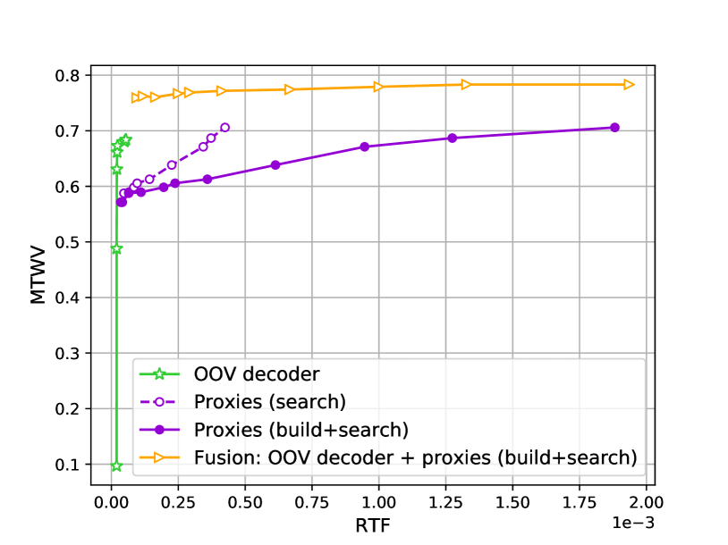
Figure 1: Comparison of two approaches for OOV KWS: (1) OOV decoder and (2) proxies and their fusion for results from the fusion of the 9 ASR systems

In addition to the lattice-level fusion, we performed fusion on the list-level, described in [33], using Kaldi [26] for all AMs for each approach independently and for the both approaches together (Table 2). The list-level combination of all the systems for both approaches provides an additional improvement in overall accuracy (MTWV=0.795), which corresponds to 7.4% of relative MTWV improvement over the best fusion result.

Exploration of the two main parameters of the OOV decoder (smoothing weight $\alpha$ and minimum score threshold $\Theta_{hit}$) is presented in Figures 2(a) and 2(b). The results are given for the best AM (DNN₂), for the worst AM (DMN₉) and for the lattice-based fusion of all AMs.

Table 2: Fusion results approaches for two OOV KWS approaches in terms of MTWV metric

Fusion	OOV decoder	Proxies
Lattices	0.684	0.706
Lists	0.740	0.682
Lists (for all systems)	0.795

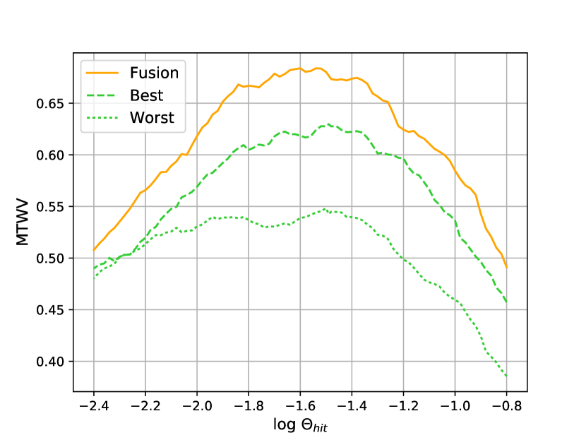
(a)

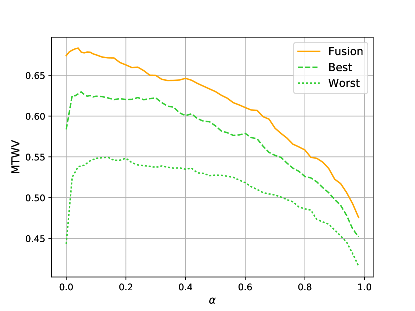
(b)

Figure 2: Dependence of the KWS accuracy for OOV decoder on parameters: (a) $\Theta_{hit}$ – minimum score threshold, and (b) $\alpha$  – smoothing weight

5 Conclusions

We have presented a novel approach for OOV keywords detection. This approach utilizes the phoneme posterior based features for decoding. Experimental results have demonstrated that in terms of MTWV metric and computational speed, for single ASR systems and for the list-level fusion of the results obtained from multiple ASR systems, the proposed algorithm significantly outperforms the proxy-based approach and provides in average 18.1% of relative MTWV improvement. The combination of the OOV decoder and proxy-based search provides an additional gain of 12.6% relative MTWV improvement over the best result obtained from the fusion results for the proxy-based method. The OOV decoder works 23-43 times faster than the proxy-based search in the point of comparable MTWV values. We have found that the combination of the two KWS methods provides an effective search strategy – a high KWS accuracy can be reached with a low RTF. The analysis of the parameters of the OOV decoder shows that the feature smoothing allows us to significantly improve the accuracy of OOV word search, what is especially important in the case of sparse lattices. Also the minimum score threshold parameter has a strong impact on MTWV and has to be optimized. In comparison with the proxy-based search the OOV decoder requires extremely low memory consumption and is very simple in implementation and parameter optimization.

6 Acknowledgements

The work was financially supported by the Ministry of Education and Science of the Russian Federation. Contract 14.579.21.0121, ID RFMEFI57915X0121.

This effort uses the IARPA Babel Program language collection release IARPA-babel{101b-v0.4c, 102b-v0.5a, 103b-v0.4b, 201b-v0.2b, 203b-v3.1a, 205b-v1.0a, 206b-v0.1e, 207b-v1.0e, 301b-v2.0b, 302b-v1.0a, 303b-v1.0a, 304b-v1.0b, 305b-v1.0c, 306b-v2.0c, 307b-v1.0b, 401b-v2.0b, 402b-v1.0b, 403b-v1.0b, 404b-v1.0a}, set of training transcriptions and BBN part of clean web data for Georgian language.

References

- [1] L. Mangu, E. Brill, and A. Stolcke, “Finding consensus in speech recognition: word error minimization and other applications of confusion networks,” Computer Speech & Language, vol. 14, no. 4, pp. 373–400, 2000.
- [2] I. Szoke, L. Burget, J. Cernocky, and M. Fapso, “Sub-word modeling of out of vocabulary words in spoken term detection,” in 2008 IEEE Spoken Language Technology Workshop, Dec 2008, pp. 273–276.
- [3] W. Hartmann, V. B. Le, A. Messaoudi, L. Lamel, and J.-L. Gauvain, “Comparing decoding strategies for subword-based keyword spotting in low-resourced languages.” in Interspeech, 2014, pp. 2764–2768.
- [4] I. Bulyko, J. Herrero, C. Mihelich, and O. Kimball, “Subword speech recognition for detection of unseen words,” in Thirteenth Annual Conference of the International Speech Communication Association, Interspeech, 2012.
- [5] D. Karakos and R. M. Schwartz, “Subword and phonetic search for detecting out-of-vocabulary keywords.” in Interspeech, 2014, pp. 2469–2473.
- [6] Y. He, P. Baumann, H. Fang, B. Hutchinson, A. Jaech, M. Ostendorf, E. Fosler-Lussier, and J. Pierrehumbert, “Using pronunciation-based morphological subword units to improve OOV handling in keyword search,” IEEE/ACM Transactions on Audio, Speech, and Language Processing, vol. 24, no. 1, pp. 79–92, Jan 2016.
- [7] P. Yu and F. T. B. Seide, “A hybrid word/phoneme-based approach for improved vocabulary-independent search in spontaneous speech.” in Interspeech. Citeseer, 2004.
- [8] F. Seide, P. Yu, C. Ma, and E. Chang, “Vocabulary-independent search in spontaneous speech,” in Acoustics, Speech, and Signal Processing, 2004. Proceedings.(ICASSP’04). IEEE International Conference on, vol. 1. IEEE, 2004, pp. I–253.
- [9] S.-w. Lee, K. Tanaka, and Y. Itoh, “Generating complementary acoustic model spaces in DNN-based sequence-to-frame DTW scheme for out-of-vocabulary spoken term detection,” Interspeech 2016, pp. 755–759, 2016.
- [10] B. Logan and J.-M. Van Thong, “Confusion-based query expansion for oov words in spoken document retrieval.” in Interspeech, 2002.
- [11] G. Chen, O. Yilmaz, J. Trmal, D. Povey, and S. Khudanpur, “Using proxies for oov keywords in the keyword search task,” in Automatic Speech Recognition and Understanding (ASRU), 2013 IEEE Workshop on. IEEE, 2013, pp. 416–421.
- [12] L. Mangu, B. Kingsbury, H. Soltau, H.-K. Kuo, and M. Picheny, “Efficient spoken term detection using confusion networks,” in Acoustics, Speech and Signal Processing (ICASSP), 2014 IEEE International Conference on. IEEE, 2014, pp. 7844–7848.
- [13] M. Saraclar, A. Sethy, B. Ramabhadran, L. Mangu, J. Cui, X. Cui, B. Kingsbury, and J. Mamou, “An empirical study of confusion modeling in keyword search for low resource languages,” in 2013 IEEE Workshop on Automatic Speech Recognition and Understanding, Dec 2013, pp. 464–469.
- [14] D. R. Miller, M. Kleber, C.-L. Kao, O. Kimball, T. Colthurst, S. A. Lowe, R. M. Schwartz, and H. Gish, “Rapid and accurate spoken term detection.”
- [15] P. Karanasou, L. Burget, D. Vergyri, M. Akbacak, and A. Mandal, “Discriminatively trained phoneme confusion model for keyword spotting.” in Interspeech, 2012, pp. 2434–2437.
- [16] B. Logan, J.-M. Van Thong, and P. J. Moreno, “Approaches to reduce the effects of oov queries on indexed spoken audio,” IEEE transactions on multimedia, vol. 7, no. 5, pp. 899–906, 2005.
- [17] J. Mamou and B. Ramabhadran, “Phonetic query expansion for spoken document retrieval.” in Interspeech, 2008, pp. 2106–2109.
- [18] Y. Khokhlov, I. Medennikov, A. Romanenko, V. Mendelev, M. Korenevsky, A. Prudnikov, N. Tomashenko, and A. Zatvornitsky, “The STC keyword search system for OpenKWS 2016 evaluation.” in Interspeech, 2017.
- [19] L. Uebel and P. C. Woodland, “Improvements in linear transform based speaker adaptation,” in Proc. ICASSP, 2001, pp. 49–52.
- [20] C. Gollan and M. Bacchiani, “Confidence scores for acoustic model adaptation,” in Proc. ICASSP, 2008, pp. 4289–4292.
- [21] G. Evermann and P. C. Woodland, “Large vocabulary decoding and confidence estimation using word posterior probabilities,” in Acoustics, Speech, and Signal Processing, 2000. ICASSP’00. Proceedings. 2000 IEEE International Conference on, vol. 3. IEEE, 2000, pp. 1655–1658.
- [22] J. Foote, S. J. Young, G. J. Jones, and K. S. Jones, “Unconstrained keyword spotting using phone lattices with application to spoken document retrieval,” Computer Speech & Language, vol. 11, no. 3, pp. 207–224, 1997.
- [23] I. Szöke, P. Schwarz, P. Matejka, L. Burget, M. Karafiát, M. Fapso, and J. Cernockỳ, “Comparison of keyword spotting approaches for informal continuous speech.” in Interspeech. Citeseer, 2005, pp. 633–636.
- [24] L. Mangu, H. Soltau, H. K. Kuo, B. Kingsbury, and G. Saon, “Exploiting diversity for spoken term detection,” in 2013 IEEE International Conference on Acoustics, Speech and Signal Processing, May 2013, pp. 8282–8286.
- [25] J. Mamou, J. Cui, X. Cui, M. J. Gales, B. Kingsbury, K. Knill, L. Mangu, D. Nolden, M. Picheny, B. Ramabhadran et al., “System combination and score normalization for spoken term detection,” in Acoustics, Speech and Signal Processing (ICASSP), 2013 IEEE International Conference on. IEEE, 2013, pp. 8272–8276.
- [26] D. Povey, A. Ghoshal, G. Boulianne, L. Burget, O. Glembek, N. Goel, M. Hannemann, P. Motlicek, Y. Qian, P. Schwarz et al., “The kaldi speech recognition toolkit,” in IEEE 2011 workshop on automatic speech recognition and understanding, no. EPFL-CONF-192584. IEEE Signal Processing Society, 2011.
- [27] V. Peddinti, D. Povey, and S. Khudanpur, “A time delay neural network architecture for efficient modeling of long temporal contexts.” in Interspeech, 2015, pp. 3214–3218.
- [28] T. Ko, V. Peddinti, D. Povey, and S. Khudanpur, “Audio augmentation for speech recognition.” in Interspeech, 2015, pp. 3586–3589.
- [29] A. Stolcke, “SRILM-an extensible language modeling toolkit.” in 7th International Conference on Spoken Language Processing, ICSLP, vol. 2002, 2002, p. 2002.
- [30] A. Karpathy, “The unreasonable effectiveness of recurrent neural networks,” http://karpathy.github.io/2015/05/21/rnn-effectiveness, 2015.
- [31] J. Cui, J. Mamou, B. Kingsbury, and B. Ramabhadran, “Automatic keyword selection for keyword search development and tuning,” in Acoustics, Speech and Signal Processing (ICASSP), 2014 IEEE International Conference on. IEEE, 2014, pp. 7839–7843.
- [32] J. Fiscus, J. Ajot, and G. Doddington, “The spoken term detection (STD) 2006 evaluation plan,” NIST USA, Sep, 2006.
- [33] J. Trmal, G. Chen, D. Povey, S. Khudanpur, P. Ghahremani, X. Zhang, V. Manohar, C. Liu, A. Jansen, D. Klakow et al., “A keyword search system using open source software,” in Spoken Language Technology Workshop (SLT), 2014 IEEE. IEEE, 2014, pp. 530–535.