Limit Cycles of Dynamic Systems under Random Perturbations with Rapid Switching and Slow Diffusion: A Multi-Scale Approach

Abstract

This work is devoted to examining qualitative properties of dynamic systems, in particular, limit cycles of stochastic differential equations with both rapid switching and small diffusion. The systems are featured by multi-scale formulation, highlighted by the presence of two small parameters $\varepsilon$ and $\delta$. Associated with the underlying systems, there are averaged or limit systems. Suppose that for each pair of the parameters, the solution of the corresponding equation has an invariant probability measure $\mu^{\varepsilon,\delta}$, and that the averaged equation has a limit cycle in which there is an averaged occupation measure $\mu^{0}$ for the averaged equation. Our main effort is to prove that $\mu^{\varepsilon,\delta}$ converges weakly to $\mu^{0}$ as $\varepsilon\to 0$ and $\delta\to 0$ under suitable conditions. Moreover, our results are applied to a stochastic predator-prey model together with numerical examples for demonstration.

Keywords. Invariant probability measure; hybrid diffusion, rapid switching; limit cycle; predator-prey model.

Mathematics Subject Classification. 34C05, 60H10, 92D25.

1 Introduction

It is widely recognized that the traditional dynamical systems given by deterministic differential equations are often inadequate to model many natural phenomena because more often than not the systems are affected by a variety of random perturbations. For this reason, various random noise processes have been taken into consideration. Among them, diffusion processes are one of the most popular models. If the intensity of the diffusion is small, the diffusion process can be approximated by an ordinary differential equation. Consider a stochastic differential equation

$$dx^{\varepsilon}(t)=f(x^{\varepsilon}(t))dt+\sqrt{\varepsilon}\sigma(x^{\varepsilon}(t))dW(t)$$ (1.1)

for appropriate functions $f(\cdot)$ and $\sigma(\cdot)$, where $W(\cdot)$ is a standard Brownian motion and $\varepsilon$ is a small parameter. It is intuitive that as $\varepsilon\to 0$, (1.1) should have a limit that is represented by a purely deterministic differential equation. Building on using averaging ideas, in [4], Fleming considered the associated asymptotic expansions of the expectation $\mathbb{E}_{x}\Phi(x^{\varepsilon}(t))$ for a suitable function $\Phi(\cdot)$ under appropriate conditions. If the process $x^{\varepsilon}(t)$ has a unique ergodic measure $\mu^{\varepsilon}$ for each $\varepsilon>0$ and the origin of the corresponding deterministic equation

$$dx=f(x)dt,$$ (1.2)

is a globally asymptotic equilibrium point, Holland [9] established asymptotic expansions of the expectation of the underlying functionals with respect to the unique ergodic measure $\mu^{\varepsilon}$. Furthermore, in [10], he considered the case that (1.2) has an asymptotically stable limit cycle and proved the weak convergence of the unique ergodic measure $\mu^{\varepsilon}$ of $x^{\varepsilon}(t)$ to the stationary distribution of (1.2) concentrated on the limit cycle.

In recent years, to enlarge the applicability, resurgent efforts have been devoted to modeling dynamic systems in which continuous dynamics and discrete events coexist. Such “hybrid” systems arise from traditional applications in engineering, operations research, biological, and physical sciences as well as from emerging applications in wireless communications, internet traffic modeling, and financial engineering among others; see [22] and references therein. As a result, switching diffusion processes have received much attention lately. For such models, it is important to consider perturbed dynamic systems similar to that of the aforementioned paragraphs. In the literature, to take advantages of the time-scale separation, Simon and Ando [20] introduced the so-called hierarchical decomposition and aggregation as well as nearly decomposable models with economics applications; Sethi and Zhang [18] initiated the study of near-optimal controls for flexible manufacturing systems. A multi-scale approach with applications to computing and Monte Carlo simulation was treated in Liu [13]; applications of controlled dynamic systems can also be found in [8] and references therein. Recently, effort has also been devoted to treat non-autonomous lattice systems with switching in Han and Kloeden [5]. Related works have also been devoted to attraction, stability, and robustness of functional stochastic differential equations in Wu and Hu [21] and to chemical reaction systems with two-time scales in Han and Najm [6].

In this paper, we consider dynamic systems represented by switching diffusions, where the switching is rapidly varying whereas the diffusion is slowly changing. To be more precise, let $(\Omega,\mathcal{F},\{\mathcal{F}_{t}\},\mathbb{P})$ be a filtered probability space satisfying the usual condition. Consider the process

$$dX^{\varepsilon,\delta}(t)=f(X^{\varepsilon,\delta}(t),\alpha^{\varepsilon}(t))dt+\sqrt{\delta}\sigma(X^{\varepsilon,\delta}(t),\alpha^{\varepsilon}(t))dW(t),\ X^{\varepsilon}(0)=x,$$ (1.3)

where $W(t)$ is an $m$-dimensional standard Brownian motion, $\alpha^{\varepsilon}(t)$ is a Markov chain that is independent of $W(t)$ and that has a finite state space $\mathcal{M}=\{1,...,m_{0}\}$ and generator $Q/\varepsilon=\big{(}q_{ij}/\varepsilon\big{)}_{m_{0}\times m_{0}}$, $X^{\varepsilon,\delta}$ is an $\mathbb{R}^{d}$-valued process, $f:\mathbb{R}^{d}\times\mathcal{M}\to\mathbb{R}^{d},\sigma:\mathbb{R}^{d}\times\mathcal{M}\to\mathbb{R}^{d\times m},$ and $\varepsilon>0$ and $\delta>0$ are two small parameters. Assume that $Q$ is irreducible. The irreducibility of $Q$ implies that the Markov chain associated with $Q$ (denoted by $\tilde{\alpha}(t)$) is ergodic, with a unique stationary distribution $(\nu_{1},...,\nu_{m_{0}})$. Intuitively, when $\varepsilon$ and $\delta$ are very small, $\alpha^{\varepsilon}(t)$ converges rapidly to its stationary distribution and the intensity of the diffusion is negligible. As a result, on each finite interval of $t$, a solution of equation (1.3) can be approximated by

$$dX(t)=\overline{f}(X(t))dt,\ X(0)=x,$$ (1.4)

where $\overline{f}(x)=\sum_{i=1}^{m_{0}}f(x,i)\nu_{i}$. However, if in lieu of a finite interval, we consider the process in the infinite interval $[0,+\infty)$. The corresponding results could be considerably different. Suppose that equation (1.4) has a stable limit cycle, a natural question is whether invariant measures to the process represented by solution of (1.3) converge weakly to the measure concentrated on the limit cycle. To address this question, we substantially extend the results of [10] by considering the presence of both small diffusion and rapid switching. Moreover, because of the complexity due to the presence of the switching and coupling, new mathematical techniques need to be introduced to deal with the current problem. In addition, even we only consider the problem as that of [10], it will be seen later that some of our assumptions are weaker than those used in [10].

The rest of the paper is organized as follows. The main assumptions are given in Section 2. Some auxiliary results are also presented. Section 3 takes up the issue of estimation for the exit time of the solution from critical points that is needed to prove the main result. In Section 4, we consider three cases. In each of the cases, we address the aforementioned question under suitable conditions. Section 5 deals with applications of our results to a general predator-prey model. It should be mentioned that the applications are not straightforward. It is not easy to prove the existence and tightness of the family of invariant probability measures that are usually obtained using Lyapunov-type functions. However, the Lyapunov-type method does not work for our model. We introduce certain tools to overcome the difficulties. Finally, we provide some numerical examples in Section 6 to illustrate our results.

2 Assumptions and Preliminary Results

Throughout the paper, we denote by $A^{\prime}$ the transpose of a matrix $A$, $|\cdot|$ the Euclidean norm of vectors in $\mathbb{R}^{d}$, and $\|A\|:=\sup\{|Ax|:x\in\mathbb{R}^{d},|x|=1\}$ the operator norm of a matrix $A\in\mathbb{R}^{d\times d}$. We use notations $a\wedge b=\min\{a,b\}$ and $a\vee b=\max\{a,b\}$. Assuming in this paper that $\delta$ depends on $\varepsilon$ ($\delta=\delta(\varepsilon)$) and $\lim\limits_{\varepsilon\to 0}\delta(\varepsilon)=0$, we impose the following assumptions for equations (1.3) and (1.4).

Assumption 2.1.

1. For each $i\in\mathcal{M}$, $f(\cdot,i)$ and $\sigma(\cdot,i)$ are locally Lipschitz continuous.

2. There is an $a>0$ and a twice continuously differentiable real-valued function $\Phi(x)\geq 0$ such that $\lim\limits_{R\to\infty}\inf\{\Phi(x):|x|\geq R\}=\infty$ and that $\nabla\Phi^{\prime}(x)f(x,i)\leq a(\Phi(x)+1)$, $\forall\,(x,i)\in\mathbb{R}^{d}\times\mathcal{M}$.

3. Equation (1.4) has a unique limit cycle denoted by $\Gamma.$

4. In any compact subset of $\mathbb{R}^{d}$, there is a finite number of critical points of $\overline{f}(\cdot)$.

5. For each compact set $\mathcal{K}$ not containing any critical point of $\overline{f}$, and $\gamma>0$, there exists a $T=T_{\mathcal{K},\gamma}>0$ such that $\inf\limits_{y\in\Gamma}|\overline{X}_{x}(t)-y|<\gamma$ for all $t\geq T$.

6. There is an $\varepsilon_{0}>0$ such that for all $0<\varepsilon<\varepsilon_{0}$, there exists a unique solution to equation (1.3). The process $(X(t),\alpha^{\varepsilon,\delta}(t))$ has the strong Markov property and has an invariant measure $\mu^{\varepsilon,\delta}$. As a convention, given $A\subset\mathbb{R}^{d}$, we denote $\mu^{\varepsilon,\delta}(A\times\mathcal{M})$ by $\mu^{\varepsilon,\delta}(A)$ for convenience. The family $\{\mu^{\varepsilon,\delta}:0<\varepsilon<\varepsilon_{0}\}$ is tight in the sense that for any $\gamma>0$, there exists an $R>0$ such that $\mu^{\varepsilon,\delta}\{B_{R}\}>1-\gamma$ for all $0<\varepsilon<\varepsilon_{0}$, where $B_{R}=\{x:|x|\leq R\}$.

For simplicity, we have assumed that (1.3) has a unique solution; we have also assumed that the associated process is strong Markov. Sufficient conditions ensuring these can be provided (see [15, 22]). Since these are already known and are not our main concern here, we use the conditions as stated above. Let $T_{\Gamma}$ be the period of the limit cycle $\Gamma$. For any $y\in\Gamma$, we can define a probability measure $\mu^{0}$ (not dependent on $y$) by

$$\mu^{0}(A)=\dfrac{1}{T_{\Gamma}}\int_{0}^{T_{\Gamma}}\boldsymbol{1}_{\{\overline{X}_{y}(s)\in A\}}ds,$$

where $\overline{X}_{y}(t)$ is the solution to equation (1.4) starting at $\overline{X}(0)=y$ and $\boldsymbol{1}_{\{\cdot\}}$ is the indicator function. Thus $\mu^{0}(\cdot)$ is simply an averaged occupation measure. Recall that $\delta=\delta_{\varepsilon}$. We shall address asymptotic behavior of $\mu^{\varepsilon,\delta}$ for the following three cases:

$$\lim\limits_{\varepsilon\to 0}\dfrac{\delta}{\varepsilon}=\left\{\begin{array}[]{ll}l\in(0,\infty),&\mbox{ case 1}\\ 0,&\mbox{ case 2}\\ \infty,&\mbox{ case 3}.\end{array}\right.$$ (2.1)

The multi-scale modeling point was similar to [7] in which large deviations were considered. Here, we use such setting to study limit cycles of the associated dynamic systems. We impose additional conditions corresponding to each of the cases in (2.1). In case 2, since $\delta$ tends to $0$ much faster than $\varepsilon$, if $\delta$ is sufficiently small, then intuitively, the behavior of $X^{\varepsilon,\delta}(t)$ should be similar to $\xi^{\varepsilon}(t)$, the solution to

$$d\xi^{\varepsilon}(t)=f\big{(}\xi^{\varepsilon}(t),\alpha^{\varepsilon}(t)\big{)}dt.$$ (2.2)

Hence, if for each $i\in\mathcal{M}$, $f(x^{*},i)=0$ at a critical point $x^{*}$ of $\overline{f}$, the Dirac distribution $\delta(x-x^{*})$ is an invariant measure for $\xi^{\varepsilon}(t)$. Due to the above argument, the sequence of invariant probability measures $\mu^{\varepsilon,\delta}$ (or one of its subsequences) may converge to $\delta(x-x^{*})$. Consequently, we need to suppose that there is an $i^{*}\in\mathcal{M}$ such that $f(x^{*},i^{*})\neq 0$ in order to obtain the convergence of $\mu^{\delta,\varepsilon}$ to the measure $\mu^{0}$. Analogously, in case 3, we suppose that there exists an $i^{*}\in\mathcal{M}$ such that $\sigma(x^{*},i^{*})\neq 0$. For case 1, it is assumed that there is an $i^{*}\in\mathcal{M}$ satisfying either $\sigma(x^{*},i^{*})\neq 0$ or $f(x^{*},i^{*})\neq 0$.

The following formula is the well-known exponential martingale inequality, which will be used several times in our proofs. It asserts that

$$\mathbb{P}\left\{\sup_{t\in[0,T]}\Big{[}\int_{0}^{t}g(s)dW(s)-\dfrac{a}{2}\int_{0}^{t}g^{2}(s)ds\Big{]}>b\right\}\leq e^{-ab},$$

if $g(t)$ is a real-valued $\mathcal{F}_{t}$-adapted process and $\int_{0}^{T}g^{2}(t)dt<\infty$ almost surely (see [14, Theorem 1.7.4]).

Lemma 2.1.

For any $R,T,\gamma>0$, there is a $k_{1}=k_{1}(R,T,\gamma)>0$ such that for sufficiently small $\delta$,

$$\mathbb{P}\{|X^{\varepsilon,\delta}_{x,i}(t)-\xi^{\varepsilon}_{x,i}(t)|\geq\gamma,\ \forall 0\leq t\leq T\}<\exp\Big{(}-\dfrac{k_{1}}{\delta}\Big{)},\ \forall|x|\leq R,$$

where $X^{\varepsilon,\delta}_{x,i}(t)$ and $\xi^{\varepsilon}_{x,i}(t)$ are solutions to equations (1.3) and (2.2) with the same initial value $(x,i)$, respectively.

Proof.

By (i) and (ii) of Assumption 2.1, we can deduce the existence and boundedness of a unique solution to equation (2.2) using the Lyapunov function method. Moreover, we can find an $R_{T}>0$ such that $|\xi^{\varepsilon}_{x,i}(t)|<R_{T}-\gamma,\ \forall\,t\in[0,T]$ a.s. $\,\forall\,|x|\leq R$. Let $h(x)$ be a twice differentiable function with compact support and $h(x)=1$ if $|x|\leq R_{T}$ and $h(x)=0$ if $|x|\geq R_{T}+1$. Put $f_{h}(x,i)=h(x)f(x,i)$, $\sigma_{h}(x,i)=h(x)\sigma(x,i)$. Let $Y^{\varepsilon,\delta}_{x,i}(t)$ be the solution starting at $(x,i)$ to

$$dY(t)=f_{h}(Y(t),\alpha^{\varepsilon}(t))dt+\sqrt{\delta}\sigma_{h}(Y(t),\alpha^{\varepsilon}(t)dW(t)$$ (2.3)

Note that $Y^{\varepsilon,\delta}_{x,i}(t)=X^{\varepsilon,\delta}_{x,i}(t)$ up to the time $\zeta=\inf\{t>0:|X^{\varepsilon,\delta}_{x,i}(t)|>R_{T}\}$. Meanwhile $\xi^{\varepsilon}_{x,i}(t)$, the solution to (2.2), is also the solution to

$$dZ(t)=f_{h}(Z(t),\alpha^{\varepsilon}(t))dt$$

for $|x|\leq R$ and $0\leq t\leq T$. We have from the generalized Itô’s formula that

$$|Y {}^{\varepsilon,\delta}_{x,i}(t)-\xi^{\varepsilon}_{x,i}(t)|^{2}$$ (2.4)

$$\leq 2\int_{0}^{t}|Y^{\varepsilon,\delta}_{x,i}(s)-\xi^{\varepsilon}_{x,i}(s)|^{\prime}|f_{h}(Y^{\varepsilon,\delta}_{x,i}(s),\alpha^{\varepsilon}(s))-f_{h}(\xi^{\varepsilon}_{x,i}(s),\alpha^{\varepsilon}(s))|ds$$

$$+\int_{0}^{t}\delta\text{trace}\big{(}(\sigma_{h}\sigma_{h}^{\prime})(Y^{\varepsilon,\delta}_{x,i}(s),\alpha^{\varepsilon}(s))\big{)}ds$$

$$+2\sqrt{\delta}\left|\int_{0}^{t}\big{(}Y^{\varepsilon,\delta}_{x,i}(s)-\xi^{\varepsilon}_{x,i}(s)\big{)}^{\prime}\sigma_{h}(Y^{\varepsilon,\delta}_{x,i}(s),\alpha^{\varepsilon}(s)\big{)}dW(s)\right|.$$

By the exponential martingale inequality, for any $\delta<k_{1}$,

$$\mathbb{P}(A)\geq 1-2\exp\Big{(}-\dfrac{2k_{1}}{\delta}\Big{)}\geq 1-\exp\Big{(}-\frac{k_{1}}{\delta}\Big{)},$$

where

$$A=\bigg{\{}\omega: \Big{|}\int_{0}^{t}\sqrt{\delta}\big{(}Y^{\varepsilon,\delta}_{x,i}(s)-\xi^{\varepsilon}_{x,i}(s)\big{)}^{\prime}\sigma_{h}(Y^{\varepsilon,\delta}_{x,i}(s),\alpha^{\varepsilon}(s)\big{)}dW(s)\Big{|}$$

$$\qquad-\dfrac{1}{\delta}\int_{0}^{t}\delta\big{|}Y^{\varepsilon,\delta}_{x,i}(s)-\xi^{\varepsilon}_{x,i}(s)\big{|}^{2}\|\sigma_{h}\sigma_{h}^{\prime}(Y^{\varepsilon,\delta}_{x,i}(s),\alpha^{\varepsilon}(s)\big{)}\|ds\leq k_{1}\,\text{ for all }\,t\in[0,T]\bigg{\}}.$$

Since $f_{h}$ is Lipschitz and $\sigma_{h}$ is bounded, we have for $\omega\in A$ and some sufficiently large $M_{1}$,

$$|Y^{\varepsilon,\delta}_{x,i} (t)-\xi^{\varepsilon}_{x,i}(t)|^{2}$$ (2.5)

$$\leq 2\int_{0}^{t}|Y^{\varepsilon,\delta}_{x,i}(s)-\xi^{\varepsilon}_{x,i}(s)|^{\prime}|f_{h}(Y^{\varepsilon,\delta}_{x,i}(s),\alpha^{\varepsilon}(s))-f_{h}(\xi^{\varepsilon}_{x,i}(s),\alpha^{\varepsilon}(s))|ds$$

$$\ +2\int_{0}^{t}\big{|}Y^{\varepsilon,\delta}_{x,i}(s)-\xi^{\varepsilon}_{x,i}(s)\big{|}^{2}\|\sigma_{h}\sigma_{h}^{\prime}(Y^{\varepsilon,\delta}_{x,i}(s),\alpha^{\varepsilon}(s)\big{)}\|ds$$

$$\ +\int_{0}^{t}\delta\text{trace}\big{(}(\sigma_{h}\sigma_{h}^{\prime})(Y^{\varepsilon,\delta}_{x,i}(s),\alpha^{\varepsilon}(s))\big{)}ds+2\int_{0}^{t}k_{1}ds$$

$$\leq M_{1}\int_{0}^{t}|Y^{\varepsilon,\delta}_{x,i}(t)-\xi^{\varepsilon}_{x,i}(t)|^{2}ds+(2k_{1}+M_{1}\delta)t.$$

For each $t\in[0,T]$, Gronwall’s inequality leads to

$$|Y^{\varepsilon,\delta}_{x,i}(t)-\xi^{\varepsilon}_{x,i}(t)|^{2}\leq(2k_{1}+M_{1}\delta)T\exp(M_{1}T)<\gamma^{2}$$

for $0<\delta<k_{1}$ sufficiently small. It also follows from this inequality that for $\omega\in A$ and $0<\delta<k_{1}$ sufficient small, we have $\zeta>T$ which implies

$$|X^{\varepsilon,\delta}_{x,i}(t)-\xi^{\varepsilon}_{x,i}(t)|^{2}=|Y^{\varepsilon,\delta}_{x,i}(t)-\xi^{\varepsilon}_{x,i}(t)|^{2}<\gamma^{2},$$

$\forall 0\leq t\leq T.$ ∎

Lemma 2.2.

For each $x$ and $\gamma$, we can find $k_{\gamma,x}=k_{\gamma,x}(T)>0$ such that

$$\mathbb{P}\left\{|\xi^{\varepsilon}_{x,i}(t)-\overline{X}_{x}(t)|\geq\gamma,\ \forall 0\leq t\leq T\right\}\leq\exp\Big{(}-\frac{k_{\gamma,x}}{\varepsilon}\Big{)},$$

where $\overline{X}_{x}(t)$ is the solution to equation (1.4) with the initial value $x$.

Proof.

It follows immediately from the large deviation principle shown in [8] with a note that the existence and boundedness of a unique solution to equation (2.2) follows from (i) and (ii) of Assumption 2.1. ∎

Combining Lemmas 2.1 and 2.2, we obtain the following lemma.

Lemma 2.3.

For any $R$, $T$, $\gamma>0$, there is a $k=k(R,\gamma,T)>0$ such that

$$\mathbb{P}\left\{|X^{\varepsilon,\delta}_{x,i}(t)-\overline{X}_{x}(t)|\geq\gamma,\ \forall 0\leq t\leq T\right\}<\exp\Big{(}-\frac{k}{\varepsilon+\delta}\Big{)},\ \forall|x|\leq R.$$

Proof.

By virtue of Lemma 2.2, for each $x$ and $\gamma$, we have

$$\mathbb{P}\left\{|\xi^{\varepsilon}_{x,i}(t)-\overline{X}_{x}(t)|\geq\dfrac{\gamma}{6},\ \forall 0\leq t\leq T\right\}\leq\exp\Big{(}-\frac{k_{\gamma/6,x}}{\varepsilon}\Big{)}.$$

Using the Lyapunov method to (2.2) in view of $(ii)$ of Assumption 2.1, there is an $H_{R,T}>0$ such that $|\xi^{\varepsilon}_{x,i}(t)|\leq H_{R,T}$ and $|\overline{X}_{x}(t)|\leq H_{R,T}$ for all $|x|\leq R$ and $0\leq t\leq T$. Since $f(\cdot,i)$ is locally Lipschitz for all $i\in\mathcal{M}$, there is a constant $M_{2}>0$ such that $|f(u,i)-f(v,i)|\leq M_{2}|u-v|$ for all $|u|\vee|v|\leq H_{R,T}$ and $i\in\mathcal{M}$. Using the Gronwall inequality, we have for $|x|\vee|y|\leq R$ and $i\in\mathcal{M}$ that

$$\begin{array}[]{rl}&\!\!\!\displaystyle|\xi^{\varepsilon}_{x,i}(t)-\xi^{\varepsilon}_{y,i}(t)|\leq|x-y|\exp(M_{2}T)\mbox{ and}\\ &\!\!\!\displaystyle|\overline{X}_{x}(t)-\overline{X}_{y}(t)|\leq|x-y|\exp(M_{2}T),\ \forall t\in[0,T].\end{array}$$

Let $\lambda=\dfrac{\gamma}{6}\exp(-M_{2}T)$. It is easy to see that for $|x-y|<\lambda$,

$$\mathbb{P}\left\{|\xi^{\varepsilon}_{y,i}(t)-\overline{X}_{y}(t)|\geq\dfrac{\gamma}{2},\ \forall 0\leq t\leq T\right\}\leq\exp\Big{(}-\frac{k_{\gamma/6,x}}{\varepsilon}\Big{)}.$$

By the compactness of $\{x:|x|\leq R\}$, for $\gamma>0$, there is a $k_{2}=k_{2}(R,T,\gamma)>0$ such that for $|x|\leq R$,

$$\mathbb{P}\left\{|\xi^{\varepsilon}_{x,i}(t)-\overline{X}_{x}(t)|\geq\dfrac{\gamma}{2},\ \forall 0\leq t\leq T\right\}\leq\exp\Big{(}-\frac{k_{2}}{\varepsilon}\Big{)}.$$

Combining with Lemma 2.1, we have

$$\begin{array}[]{rl}\displaystyle\mathbb{P}\left\{|X^{\varepsilon,\delta}_{x,i}(t)-\overline{X}_{x}(t)|\geq\gamma,\ \forall 0\leq t\leq T\right\}&\!\!\!\displaystyle<\exp\Big{(}-\frac{k_{1}(R,T,\gamma/2)}{\delta}\Big{)}+\exp\Big{(}-\frac{k_{2}}{\varepsilon}\Big{)}\\ &\!\!\!\displaystyle<\exp\Big{(}-\frac{k}{\varepsilon+\delta}\Big{)}\end{array}$$

for a suitable $k$ and sufficiently small $\varepsilon$ and $\delta$. ∎

3 Probability Estimate for the First Exit Time

Let $x^{*}$ be a critical point of $\overline{f}(\cdot)$. In this section, we consider a sufficiently small neighborhood $N$ of $x^{*}$ and estimate the first time $X_{x,i}^{\varepsilon,\delta}(\cdot)$ exits from $N$, say $\tau_{x,i}^{\varepsilon,\delta}$. Since we mainly consider the time that the process exits a small neighborhood, by arguments similar to those in the proof of Lemma 2.1, we can suppose that $f$ and $\sigma$ are bounded. Let $x^{*}=0$ for convenience. Since we will assume later that there are $i^{*}\in\mathcal{M}$ and $\beta\in\mathbb{R}^{d},|\beta|=1$ such that $\beta^{\prime}f(0,i^{*})>0$ or $\beta^{\prime}\sigma(0,i^{*})>0$, we choose $c_{1}>0$ sufficient small such that $S=\{y:|y|<c_{1}\}$ contains only one critical point 0 and that for all $x\in\overline{S}=\{y:|y|\leq c_{1}\}$ we have $\beta^{\prime}f(x,i^{*})>0$ or $\beta^{\prime}\sigma(x,i^{*})>0$ depending on which function we impose the condition on. In view of (v) of Assumption 2.1, there is a $T_{c_{1}}>0$ such that $\overline{X}_{x}(t)\notin S$ for all $t>T_{c_{1}}$ and $x\in\partial S:=\{y:|y|=c_{1}\}$. It follows from the continuous dependence of solutions on initial data that there is $0<c_{2}<c_{1}$ such that $\inf\{|\overline{X}_{x}(t)|:x\in\partial S,t\in[0,T_{c_{1}}]\}>c_{2}.$ Consequently, $\inf\{\overline{X}_{x}(t):x\notin S,t\geq 0\}>c_{2}$. Similarly, we can find $0<c_{3}<\dfrac{c_{2}}{2}$ such that $\inf\{\overline{X}_{x}(t):|x|\geq c_{2},t\geq 0\}\geq 2c_{3}$. Put $N=\{y:|y|<c_{3}\}$, $G=\{y:|y|<c_{2}\}$, and let $\gamma\in\big{(}0,\min\{c_{1}-c_{2},c_{2}-2c_{3},c_{3}\}\big{)}$. Then, the following assertions are true:

• $N\subset G\subset S.$

• For any $x\notin S$, $\overline{X}_{x}(t)\notin G$ for all $t\geq 0$.

• For any $x\notin G$, $y\in N$, we have $|\overline{X}_{x}(t)-y|>\gamma,\ \forall\,t\geq 0$.

Lemma 3.1.

Suppose that there is an $\ell>0$ such that $\mathbb{P}\{\tau_{x,i}^{\varepsilon,\delta}<\ell\}\geq a^{\varepsilon,\delta}>0,\ \forall(x,i)\in N\times\mathcal{M}$, where $\lim\limits_{\varepsilon\to 0}a^{\varepsilon,\delta}=0$. Then $\mathbb{P}\left\{\tau_{x,i}^{\varepsilon,\delta}<\dfrac{\ell}{a^{\varepsilon,\delta}}\right\}>1/2$ for sufficiently small $\varepsilon$.

Proof.

Let $n^{\varepsilon,\delta}\in\mathbb{N}$ such that $n^{\varepsilon,\delta}-1<\dfrac{1}{a^{\varepsilon,\delta}}\leq n^{\varepsilon,\delta}.$ We consider events $A_{k}=\{X_{x}^{\varepsilon,\delta}(t)\in N,\ \forall(k-1)\ell<t\leq k\ell\}$. We have $\mathbb{P}(A_{1})\leq 1-a^{\varepsilon,\delta}.$ By the Markov property,

$$\begin{array}[]{rl}\displaystyle\mathbb{P}(A_{k}|A_{1},...,A_{k-1})&\!\!\!\displaystyle=\int_{N}\mathbb{P}\left\{\tau_{y}^{\varepsilon,\delta}\leq\ell\right\}\mathbb{P}\Big{\{}X_{x}^{\varepsilon,\delta}((k-1)\ell)\in dy\Big{|}A_{1},...,A_{k-1}\Big{\}}\\ &\!\!\!\displaystyle\leq 1-a^{\varepsilon,\delta}.\end{array}$$

As a result,

$$\mathbb{P}(A_{1}A_{2}\cdots A_{n})\leq(1-a^{\varepsilon,\delta})^{n^{\varepsilon,\delta}}$$

Since $\lim\limits_{\varepsilon\to 0}a^{\varepsilon,\delta}=0$, we deduce that $\lim\limits_{\varepsilon\to 0}(1-a^{\varepsilon,\delta})^{n^{\varepsilon,\delta}}=e^{-1}$, which means that $(1-a^{\varepsilon,\delta})^{n^{\varepsilon,\delta}}<1/2$ for sufficiently small $\varepsilon$. ∎

Lemma 3.2.

If there is an $i^{*}$ such that $f(0,i^{*})\neq 0$, then for any $\Delta>0$, we can find $H^{\Delta}_{1}>0$,and $\varepsilon_{1}(\Delta)$ such that for $\varepsilon<\varepsilon_{1}(\Delta)$,

$$\mathbb{P}\left\{\tau^{\varepsilon,\delta}_{x,i}\leq H^{\Delta}_{1}\exp\Big{(}\dfrac{\Delta}{\varepsilon}\Big{)}\right\}>1/2\,\forall\,(x,i)\in N\times\mathcal{M}.$$

Proof.

Let $\beta\in\mathbb{R}^{d}$, $|\beta|=1$ such that $\beta^{\prime}f(0,i^{*})>0$. Suppose that $\beta^{\prime}f(x,i^{*})>a_{1}>0$ for all $x\in S$. We need only work with a small $\Delta$, so we can suppose $h_{\Delta}:=\dfrac{a_{1}\Delta}{4|q_{i^{*}i^{*}}|}<c_{3}$. First, we consider the case $\alpha^{\varepsilon}(0)=i^{*}$. Because of the independence of $\alpha^{\varepsilon}(\cdot)$ and $W(\cdot)$, given that $\alpha^{\varepsilon}(t)=i^{*},\ \forall t\in\Big{[}0,\frac{\Delta}{|q_{i^{*}i^{*}}|}\Big{]}$, $X^{\varepsilon,\delta}_{x,i^{*}}(\cdot)$ has the same distribution on $\Big{[}0,\frac{\Delta}{|q_{i^{*}i^{*}}|}\Big{]}$ as the solution $Z^{\delta}_{x}$ of the equation

$$dZ(t)=f(Z(t),i^{*})dt+\sqrt{\delta}\sigma(Z(t),i^{*})dW(t).$$

Put

$$\rho^{\varepsilon,\delta}_{x}=\dfrac{\Delta}{|q_{i^{*}i^{*}}|}\wedge\inf\{t>0:|Z_{x}^{\delta}(t))|\geq h_{\Delta}\}.$$

If $|x|\geq h_{\Delta}$ then $\rho^{\varepsilon,\delta}_{x}=0$. Hence, we just consider the case $|x|<h_{\Delta}$. We have

$$\beta^{\prime}Z_{x}^{\delta}(\rho_{x}^{\varepsilon,\delta})=\beta^{\prime}x+\int_{0}^{\rho^{\varepsilon,\delta}_{x}}\beta^{\prime}f(Z_{x}^{\delta}(s),i^{*})ds+\int_{0}^{\rho^{\varepsilon,\delta}_{x}}\sqrt{\delta}\beta^{\prime}\sigma(Z_{x}^{\delta}(s),i^{*})dW(s).$$

By the exponential martingale inequality,

$$\begin{array}[]{rl}&\!\!\!\displaystyle\mathbb{P}\Big{\{}-\int_{0}^{\rho^{\varepsilon,\delta}_{x}}\sqrt{\delta}\beta^{\prime}\sigma(Z_{x}^{\delta}(s),i^{*})dW(s)\\ &\displaystyle\quad-\dfrac{1}{\sqrt{\delta}}\int_{0}^{\rho^{\varepsilon,\delta}_{x}}\delta\beta^{\prime}\sigma(Z_{x}^{\delta}(s),i^{*})\sigma(Z_{x}^{\delta}(s),i^{*})^{\prime}\beta ds>\sqrt{\delta}\Big{\}}\leq e^{-2}<1/2.\end{array}$$

Thus

$$\begin{array}[]{rl}&\!\!\!\displaystyle\mathbb{P}\Big{\{}\beta^{\prime}Z_{x}^{\delta}(\rho_{x}^{\varepsilon,\delta})>\beta^{\prime}x+\int_{0}^{\rho^{\varepsilon,\delta}_{x}}\beta^{\prime}f(Z_{x}^{\delta}(s),i^{*})ds\\ &\displaystyle\quad-\dfrac{1}{\sqrt{\delta}}\int_{0}^{\rho^{\varepsilon,\delta}_{x}}\beta^{\prime}\delta\sigma(Z_{x}^{\delta}(s),i^{*})^{\prime}\sigma(Z_{x}^{\delta}(s),i^{*})\beta ds-\sqrt{\delta}\Big{\}}>1/2.\end{array}$$

Consequently, there is some positive constant $M_{3}$ such that

$$\begin{array}[]{ll}&\!\!\!\displaystyle\mathbb{P}\Big{\{}|Z_{x}^{\delta}({\rho^{\varepsilon,\delta}_{x}})|\geq\beta^{\prime}Z_{x}^{\delta}({\rho^{\varepsilon,\delta}_{x}})>-|\beta||x|+\int_{0}^{\rho^{\varepsilon,\delta}_{x}}a_{1}ds-M_{3}\sqrt{\delta}\\ &\displaystyle\qquad\geq-h_{\Delta}+a_{1}{\rho^{\varepsilon,\delta}_{x}}-M_{3}\sqrt{\delta}\Big{\}}>1/2.\end{array}$$ (3.1)

Let $\delta$ be so small that $M_{3}\sqrt{\delta}<\dfrac{a_{1}}{2}\dfrac{\Delta}{|q_{i^{*}i^{*}}|}$. If $\rho^{\varepsilon,\delta}_{x}=\dfrac{\Delta}{|q_{i^{*}i^{*}}|}$, we have

$$|Z_{x}^{\delta}({\rho^{\varepsilon,\delta}_{x}})|\leq h_{\Delta}<-h_{\Delta}+a_{1}{\rho^{\varepsilon,\delta}_{x}}-M_{3}\sqrt{\delta}.$$

We claim from (3.1) and the above fact that for sufficiently small $\delta$,

$$\mathbb{P}\Big{\{}\inf\{t>0:|Z_{x}^{\delta}(t)|>h_{\Delta}\}<\dfrac{\Delta}{|q_{i^{*}i^{*}}|}\Big{\}}>1/2\,\forall x:|x|\leq h_{\Delta}$$

which implies

$$\mathbb{P}\bigg{\{}\eta^{\varepsilon,\delta}_{x,i^{*}}\leq\dfrac{\Delta}{q_{i^{*}i^{*}}}\bigg{|}\alpha(t)=i^{*},\ \forall t\in\Big{[}0,\dfrac{\Delta}{|q_{i^{*}i^{*}}|}\Big{]}\bigg{\}}>1/2\,\forall x:|x|\leq h_{\Delta},$$

where $\eta^{\varepsilon,\delta}_{x,i}=\inf\Big{\{}t:\big{|}X^{\varepsilon,\delta}_{x,i}(t)\big{|}>h_{\Delta}\Big{\}}.$ Consequently,

$$\mathbb{P}\Big{\{}\eta^{\varepsilon,\delta}_{x,i^{*}}\leq\dfrac{\Delta}{|q_{i^{*}i^{*}}|}\Big{\}}>\dfrac{1}{2}\mathbb{P}\Big{\{}\alpha^{\varepsilon}(t)=i^{*},\ \forall t\in\Big{[}0,\dfrac{\Delta}{|q_{i^{*}i^{*}}|}\Big{]}\Big{\}}=\dfrac{1}{2}\exp(-\dfrac{\Delta}{\varepsilon}).$$

Since $\alpha^{\varepsilon}(t)$ is ergodic, for any sufficiently small $\varepsilon$,

$$\mathbb{P}\{\alpha^{\varepsilon}(t)=i^{*}\mbox{ for some }t\in[0,1]|\alpha^{\varepsilon}(0)=i\}>{1\over 2},\ \forall i\in\mathcal{M}.$$

By the strong Markov property,

$$\mathbb{P}\left\{\eta^{\varepsilon,\delta}_{x,i}<1+\dfrac{\Delta}{|q_{i^{*}i^{*}}|}\right\}\geq{1\over 4}\exp\left(-\dfrac{\Delta}{\varepsilon}\right),\ \forall\,(x,i)\in N\times\mathcal{M}.$$ (3.2)

It is easy to see that if $|y|\geq h_{\Delta},$ by (v) of Assumption 2.1, there exists a $T_{h_{\Delta}}>0$ such that $\big{|}\overline{X}_{y}\big{(}T_{h_{\Delta}}\big{)}\big{|}\notin G.$ In view of Lemma 2.3, for $\varepsilon$ sufficiently small,

$$\mathbb{P}\Big{\{} \Big{|}X^{\varepsilon,\delta}_{y,i}\big{(}T_{h_{\Delta}}\big{)}-\overline{X}_{y}\big{(}T_{h_{\Delta}}\big{)}\Big{|}<\gamma\Big{\}}>{1\over 2},\ \forall y\in S,i\in\mathcal{M}.$$

Since $\overline{X}_{y}\big{(}T_{h_{\Delta}}\big{)}\notin G$, it follows from the construction of $G$ and $N$, when $\varepsilon$ is small, $\mathbb{P}\Big{\{}X^{\varepsilon,\delta}_{y,i}\big{(}T_{h_{\Delta}}\big{)}\notin N\Big{\}}>1/2$ provided that $h_{\Delta}\leq|y|\leq c_{2}.$ As a result,

$$\mathbb{P}\left\{\tau^{\varepsilon,\delta}_{y,i}<1+\dfrac{\Delta}{|q_{i^{*}i^{*}}|}+T_{h_{\Delta}}\right\}>{1\over 8}\exp\left(-\dfrac{\Delta}{\varepsilon}\right),\ \forall y\in N$$ (3.3)

Using Lemma 3.1, for sufficiently small $\varepsilon$,

$$\mathbb{P}\left\{\tau^{\varepsilon,\delta}_{x,i}<H^{\Delta}_{1}\exp\Big{(}\dfrac{\Delta}{\varepsilon}\Big{)}\right\}\geq{1\over 2}\,\forall\,(x,i)\in N\times\mathcal{M},$$

where $H^{\Delta}_{1}:=8\Big{(}1+\dfrac{\Delta}{|q_{i^{*}i^{*}}|}+T_{h_{\Delta}}\Big{)}.$ ∎

Lemma 3.3.

Suppose that $\lim\limits_{\varepsilon\to 0}{\delta\over\varepsilon}=l>0$ and $f(0,i)=0$ for all $i$, and there is an $i^{*}$ satisfying $\sigma(0,i^{*})\neq 0.$ Then, for every $\Delta>0$, there are $H^{\Delta}_{2}>0$ and $\varepsilon_{2}(\Delta)>0$ such that for $\varepsilon<\varepsilon_{2}(\Delta)$,

$$\mathbb{P}\left\{\tau^{\varepsilon,\delta}_{x,i}<H^{\Delta}_{2}\exp\Big{(}\dfrac{\Delta}{\delta}\Big{)}\right\}>1/2,\ \forall\,(x,i)\in N\times\mathcal{M}.$$

Proof.

Without loss of generality, we consider only the case $\lim\limits_{\varepsilon\to 0}{\delta\over\varepsilon}=1$. $\sigma(0,i^{*})\neq 0$ implies that there is $\beta\in\mathbb{R}^{d}$, $|\beta|=1$ such that $\beta^{\prime}\sigma(0,i^{*})>0$. Suppose that $0<a_{2}<\beta^{\prime}(\sigma\sigma^{\prime})(y,i^{*})\beta$, $\forall y\in S$. Define

$$\zeta_{t}:=\inf\Big{\{}u>0:\int_{0}^{u}\beta^{\prime}(\sigma\sigma^{\prime})\big{(}X^{\varepsilon,\delta}_{x,i}(s\wedge\tau^{\varepsilon,\delta}_{x,i}),\alpha^{\varepsilon}(s\wedge\tau^{\varepsilon,\delta}_{x,i})\big{)}\beta ds\geq t\Big{\}}.$$

Then for all $t$, $\zeta_{t}<\infty$ a.s. and

$$M(t)=\int_{0}^{\zeta_{t}}\beta^{\prime}\sigma\big{(}X^{\varepsilon,\delta}_{x,i}(s\wedge\tau^{\varepsilon,\delta}_{x,i}),\alpha^{\varepsilon}(s\wedge\tau^{\varepsilon,\delta}_{x,i})\big{)}dW(s)$$

is a Brownian motion. This claim stems from the fact that $M(t)$ is a continuous martingale with quadratic variation $t$. Since $M(1)$ is standard normally distributed, for $\Delta<1$ and $\delta$ is sufficiently small, we have the estimate

$$\mathbb{P}\{\sqrt{\delta}M(1)>\Delta\}\geq\dfrac{1}{2}\exp\Big{(}-\dfrac{\Delta}{\delta}\Big{)}.$$

Using the large deviation principle (see [8]), we claim that there is $a_{3}=a_{3}(T)>0$ such that

$$\mathbb{P}\left\{\dfrac{1}{T}\int_{0}^{T}\boldsymbol{1}_{\{\alpha^{\varepsilon}(s)=i^{*}\}}ds>\dfrac{\nu_{i^{*}}}{2}\right\}\geq 1-\exp\left(-\dfrac{a_{3}}{\varepsilon}\right).$$

Let $T,\Delta$ be such that $\dfrac{a_{2}\nu_{i^{*}}T}{2}>1$ and $\Delta<a_{3}$. Since $\lim\limits_{\varepsilon\to 0}{\delta\over\varepsilon}=1$, for sufficiently small $\varepsilon$ we have

$$\begin{array}[]{rl}&\!\!\!\displaystyle\mathbb{P}\left\{\int_{0}^{T}\beta^{\prime}(\sigma\sigma^{\prime})(X^{\varepsilon,\delta}_{x,i}(s\wedge\tau^{\varepsilon,\delta}_{x,i}))\beta ds\geq\dfrac{a_{2}\nu_{i^{*}}T}{2}\right\}\geq 1-\exp\left(-\dfrac{a_{3}}{\varepsilon}\right)\geq 1-\dfrac{1}{4}\exp\left(-\dfrac{\Delta}{\delta}\right),\end{array}$$

so

$$\mathbb{P}\{\zeta_{1}\leq T\}\geq 1-\dfrac{1}{4}\exp\left(-\dfrac{\Delta}{\delta}\right).$$

Since $f(0,i)=0,\ \forall i\in\mathcal{M}$, we can find a $\theta=\theta(\Delta)>0$ such that $\{y:|y|\leq\theta\}\subset N$ and that $2\theta+T\times\sup\limits_{|x|<\theta,i\in\mathcal{M}}\{|f(x,i)|\}<\Delta.$ Let $\eta^{\theta}_{x,i}=\inf\{t>0:|X^{\varepsilon,\delta}_{x,i}(t)|\geq\theta\}$. Consider only the case $|x|<\theta$. Note that if $\sqrt{\delta}M(1)>\Delta$ and $\zeta_{1}\leq T$, we must have $\eta^{\theta}_{x,i}<\zeta_{1}\leq T.$ Indeed, if the three events $\{\sqrt{\delta}M(1)>\Delta\}$, $\{\zeta_{1}\leq T\}$, and $\{\eta^{\theta}_{x,i}\geq\zeta_{1}\}$ happen simultaneously, it results in a contradiction that

$$\Delta <\sqrt{\delta}M(1)=\sqrt{\delta}\int_{0}^{\zeta_{1}}\beta^{\prime}\sigma(X^{\varepsilon,\delta}_{x,i}(s),\alpha^{\varepsilon}(s))dW(s)$$

$$\leq|\beta^{\prime}X^{\varepsilon,\delta}_{x,i}(\zeta_{1})|+|\beta^{\prime}x|+\Big{|}\int_{0}^{\zeta_{1}}\beta^{\prime}f(X^{\varepsilon,\delta}_{x,i}(s),\alpha^{\varepsilon}(s))ds\Big{|}$$

$$\leq 2\theta+\int_{0}^{\zeta_{1}}|f(X^{\varepsilon,\delta}_{x,i}(s),\alpha^{\varepsilon}(s))|ds<\Delta.$$

Thus

$$\mathbb{P}\{\eta^{\theta}_{x,i}<T\}\geq\mathbb{P}\{\sqrt{\delta}M(1)>\Delta,\zeta_{1}\leq T\}\geq\dfrac{1}{4}\exp(-\dfrac{\Delta}{\delta})\,\forall\,|x|<\theta,i\in\mathcal{M}.$$ (3.4)

By (v) of Assumption 2.1, there is a $T_{\theta}$ such that $|\overline{X}_{y}(T_{\theta})|\geq c_{2}$ for all $y$ satisfying $|y|\geq\theta$. In view of Lemma 2.3, when $\varepsilon$ is sufficiently small, for all $\theta\leq|y|\leq c_{2}$,

$$\mathbb{P}\{\tau^{\varepsilon,\delta}_{y,i}<T_{\theta}\}\geq\mathbb{P}\big{\{}\big{|}X^{\varepsilon,\delta}_{y,i}(T_{\theta})-\overline{X}_{y}(T_{\theta})\big{|}<\gamma\big{\}}>1/2.$$ (3.5)

Applying the strong Markov property, (3.4) and (3.5) yield

$$\mathbb{P}\big{\{}\tau^{\varepsilon,\delta}_{x,i}\leq T+T_{\theta}\big{\}}\geq\dfrac{1}{8}\exp\Big{(}-\dfrac{\Delta}{\delta}\Big{)}\,\forall\,(x,i)\in N\times\mathcal{M}.$$

Let $H^{\Delta}_{2}:=8(T+T_{\theta}).$ Then it follows from Lemma 3.1 that when $\varepsilon<\varepsilon_{2}(\Delta)$ for some positive $\varepsilon_{2}(\Delta)$,

$$\mathbb{P}\Big{\{}\tau^{\varepsilon,\delta}_{x,i}\leq H^{\Delta}_{2}\exp(\dfrac{\Delta}{\delta})\Big{\}}\geq{1\over 2}\,\forall\,(x,i)\in N\times\mathcal{M}.$$ (3.6)

∎

Lemma 3.4.

Suppose that $\lim\limits_{\varepsilon\to 0}\dfrac{\delta}{\varepsilon}=\infty$. Moreover, $\sigma(0,i^{*})\neq 0$. For every $\Delta>0$, there is an $H^{\Delta}_{3}>0$ and an $\varepsilon_{3}(\Delta)>0$ such that for $\varepsilon<\varepsilon_{3}(\Delta)$,

$$\mathbb{P}\Big{\{}\tau^{\varepsilon,\delta}_{x,i}<H^{\Delta}_{3}\exp\big{(}\dfrac{\Delta}{\delta}\big{)}\Big{\}}>\frac{1}{2}\,\forall\,(x,i)\in N\times\mathcal{M}.$$

Proof.

Let $a_{2},M(t),T,\zeta_{1}$ be as in the proof of Lemma 3.3. We have

$$\mathbb{P}\big{\{}\zeta_{1}\leq T\big{\}}\geq 1-\exp\Big{(}-\dfrac{a_{3}}{\varepsilon}\Big{)}\ \hbox{ for some }\ a_{3}>0.$$

Since $\overline{f}(0)=0$, we can apply the large deviation principle (see [8]) to show that there is $\kappa=\kappa(\Delta)>0$ satisfying

$$\mathbb{P}\big{\{}A\big{\}}\geq 1-\exp\Big{\{}-\dfrac{\kappa}{\varepsilon}\Big{\}}\mbox{ where }A=\left\{\left|\int_{0}^{u}f(0,\alpha^{\varepsilon}(s))ds\right|<\dfrac{\Delta}{2},\ \forall 0\leq u\leq T\right\}.$$

We can choose $\theta=\theta(\Delta)>0$ such that $\{y:|y|\leq\theta\}\subset N$ and that

$$2\theta+T\times\sup\limits_{|x|<\theta}\{|f(x,i)-f(0,i)|\}<\dfrac{\Delta}{2}.$$

Note that

$$\begin{array}[]{rl}M(1)&\!\!\!\displaystyle=\int_{0}^{\zeta_{1}}\beta^{\prime}\sigma(X^{\varepsilon,\delta}_{x,i}(s),\alpha^{\varepsilon}(s))dW(s)\\ &\!\!\!\displaystyle\leq|\beta^{\prime}X^{\varepsilon,\delta}_{x,i}(\zeta_{1})|+|\beta^{\prime}x|+\Big{|}\int_{0}^{\zeta_{1}}\beta^{\prime}f(0,\alpha^{\varepsilon}(s))ds\Big{|}\\ &\displaystyle\ +\int_{0}^{\zeta_{1}}\big{|}\beta^{\prime}\big{(}f(X^{\varepsilon,\delta}_{x,i}(s),\alpha^{\varepsilon}(s))-f(0,\alpha^{\varepsilon}(s))\big{)}\big{|}ds.\end{array}$$

Using arguments similar to those in the proof of Lemma 3.3, we can prove that

$$\{\eta^{\theta}_{x,i}\leq T\}\supset\{\sqrt{\delta}M(1)>\Delta\}\cap A\,\forall\,|x|<\theta,i\in\mathcal{M}.$$

Since $\mathbb{P}\{\delta M(1)>\Delta\}\geq\dfrac{1}{2}\exp\Big{(}-\dfrac{\Delta}{\delta}\Big{)}$, we have

$$\mathbb{P}\Big{\{}\eta^{\theta}_{x,i}<T\Big{\}} \geq\mathbb{P}\{\sqrt{\delta}M(1)>\Delta\}-\big{(}1-\mathbb{P}(A)\big{)}$$

$$\geq\dfrac{1}{2}\exp\big{(}-\dfrac{\Delta}{\delta}\big{)}-\exp\Big{(}-\dfrac{\kappa}{\varepsilon}\Big{)}\,\forall\,|x|<\theta,i\in\mathcal{M}.$$

It follows from the hypothesis $\lim\limits_{\varepsilon\to 0}\dfrac{\delta}{\varepsilon}=0$ that

$$\mathbb{P}\big{\{}\eta^{\theta}_{x,i}<T\big{\}}\geq\dfrac{1}{4}\exp\Big{(}-\dfrac{\Delta}{\delta}\Big{)}\,\forall\,|x|<\theta,i\in\mathcal{M}$$

for sufficiently small $\varepsilon$. The desired result now can be obtained similar to that of the proof of Lemma 3.3. ∎

4 Three Cases

This section provides the proofs of the convergence of $\mu^{\varepsilon,\delta}$ for the three cases given in (2.1). We first state the respective assumptions needed.

Assumption 4.1.

Assume $\lim\limits_{\varepsilon\to 0}\dfrac{\delta}{\varepsilon}=l>0$. Suppose further that for any critical point $x^{*}$ of $\overline{f}(x)$, there is an $i^{*}$ such that either $f(x^{*},i^{*})\neq 0$ or $\sigma(x^{*},i^{*})\neq 0$. In what follows, we suppose without loss of generality that $l=1$.

Assumption 4.2.

Assume $\lim\limits_{\varepsilon\to 0}\dfrac{\delta}{\varepsilon}=0$. Moreover, for any critical point $x^{*}$ of $\overline{f}(x)$, there is an $i^{*}$ such that $f(x^{*},i^{*})\neq 0$.

Assumption 4.3.

Assume $\lim\limits_{\varepsilon\to 0}\dfrac{\delta}{\varepsilon}=\infty$. Furthermore, for any critical point $x^{*}$ of $\overline{f}(x)$, there is an $i^{*}$ such that $\sigma(x^{*},i^{*})\neq 0$.

Having estimates in Section 3, we develop techniques in [10] to prove that for any critical point $x^{*}$, if one of the three above assumption holds, there is a neighborhood $N_{x^{*}}$ such that $\lim\limits_{\varepsilon\to 0}\mu^{\varepsilon,\delta}(N_{x^{*}})=0$. We suppose that $x^{*}=0$ and $S,N,G,\gamma$ are defined as in Section 3. Assume that $\limsup\limits_{\varepsilon\to 0}\mu^{\varepsilon,\delta}(N)>\vartheta>0$. Let $R$ be so large that $\mu^{\varepsilon,\delta}(B_{R})>1-\dfrac{\vartheta}{2}$ and that $B_{R-\gamma}$ contains all critical points and the limit cycle $\Gamma$. By (v) of Assumption 2.1, we can let $\hat{T}$ be such that

$$\overline{X}_{x}(\hat{T}) \in B_{R-\gamma}\setminus S,\ \forall x\in B_{R}\setminus N.$$ (4.1)

Recall that there is a $k=k(R)>0$ such that for $\varepsilon$ sufficiently small,

$$\mathbb{P}\left\{|X^{\varepsilon,\delta}_{x,i}(\hat{T})-\overline{X}_{x}(\hat{T})|\geq\gamma\right\}<\exp\Big{(}-\dfrac{k}{\varepsilon+\delta}\Big{)},\ \forall|x|\leq R.$$ (4.2)

Choose $\Delta<k/2$ and denote $T_{\Delta}^{\varepsilon,\delta}=H^{\Delta}_{j}\exp\big{(}\dfrac{\Delta}{\varepsilon}\big{)}$ or $T_{\Delta}^{\varepsilon,\delta}=H^{\Delta}_{j}\exp\big{(}\dfrac{\Delta}{\delta}\big{)}$ $(j=1,2$ or $3)$ as in Lemma 3.2, Lemma 3.3, or Lemma 3.4 depending on the case we are considering. Clearly, $T_{\Delta}^{\varepsilon,\delta}\exp(-\dfrac{k}{\varepsilon+\delta})\to 0$ as $\varepsilon\to 0$. Let $\widetilde{X}^{\varepsilon,\delta}(t)$ be the stationary solution, whose distribution is $\mu^{\varepsilon,\delta}$ at every $t$. Let $\tau^{\varepsilon,\delta}$ be the first exit time of $\widetilde{X}^{\varepsilon,\delta}(t)$ from $N$. Define events

$$K_{1}^{\varepsilon,\delta} =\Big{\{}\widetilde{X}^{\varepsilon,\delta}(T_{\Delta}^{\varepsilon,\delta})\in N,\tau^{\varepsilon,\delta}\geq T_{\Delta}^{\varepsilon,\delta},\widetilde{X}^{\varepsilon,\delta}(0)\in N\Big{\}}$$

$$K_{2}^{\varepsilon,\delta} =\Big{\{}\widetilde{X}^{\varepsilon,\delta}(T_{\Delta}^{\varepsilon,\delta})\in N,\tau^{\varepsilon,\delta}<T_{\Delta}^{\varepsilon,\delta},\widetilde{X}^{\varepsilon,\delta}(0)\in N\Big{\}}$$

$$K_{3}^{\varepsilon,\delta} =\Big{\{}\widetilde{X}^{\varepsilon,\delta}(T_{\Delta}^{\varepsilon,\delta})\in N,\widetilde{X}^{\varepsilon,\delta}(0)\in B_{R}\setminus N\Big{\}}$$

$$K_{4}^{\varepsilon,\delta} =\Big{\{}\widetilde{X}^{\varepsilon,\delta}(T_{\Delta}^{\varepsilon,\delta})\in N,\widetilde{X}^{\varepsilon,\delta}(0)\notin B_{R}\Big{\}}.$$

Note that $\mu^{\varepsilon,\delta}(N)=\sum_{n=1}^{4}\mathbb{P}\{K_{n}^{\varepsilon,\delta}\}.$ We have

$$\mathbb{P}(K_{1}^{\varepsilon,\delta})\leq\dfrac{1}{2}\mu^{\varepsilon,\delta}(N)\ \hbox{ and }\ \mathbb{P}(K_{4}^{\varepsilon,\delta})<\dfrac{\vartheta}{2}.$$

Now we estimate $\mathbb{P}(K_{3}^{\varepsilon,\delta}).$ It follows from (4.1) and (4.2) that $\mathbb{P}\{X^{\varepsilon,\delta}_{x,i}(\hat{T})\in B_{R}\setminus G\}\geq 1-\exp(-\dfrac{k}{\varepsilon+\delta})$ if $x\in B_{R}\setminus N$. Moreover, if $x\in B_{R}\setminus G$, $|\overline{X}_{x}(t)|\geq 2c_{2}\geq c_{2}+\gamma,\ \forall t\geq 0$ which implies that

$$\mathbb{P}\left\{X^{\varepsilon,\delta}_{x,i}(t)\notin N,\ \forall 0\leq t\leq\hat{T}\right\}\geq 1-\exp\Big{(}-\dfrac{k}{\varepsilon+\delta}\Big{)}.$$

Using the Markov property, for any $x\in B_{R}\setminus N,i\in\mathcal{M}$

$$\mathbb{P}\Big{\{}X_{x,i}^{\varepsilon,\delta} (T_{\Delta}^{\varepsilon,\delta})\in N\Big{\}}$$ (4.3)

$$= \mathbb{P}\Big{\{}X_{x,i}^{\varepsilon,\delta}(T_{\Delta}^{\varepsilon,\delta})\in N,X_{x,i}^{\varepsilon,\delta}(\hat{T})\notin B_{R}\setminus G\Big{\}}$$

$$+\sum_{n=2}^{\lfloor T_{\Delta}^{\varepsilon,\delta}/\hat{T}\rfloor}\mathbb{P}\Big{\{}X_{x,i}^{\varepsilon,\delta}(T_{\Delta}^{\varepsilon,\delta})\in N,X_{x,i}^{\varepsilon,\delta}(n\hat{T})\notin B_{R}\setminus G,X_{x,i}^{\varepsilon,\delta}(\iota\hat{T})\in B_{R}\setminus G,\iota=1,...,n-1\Big{\}}$$

$$+\mathbb{P}\Big{\{}X_{x,i}^{\varepsilon,\delta}(T_{\Delta}^{\varepsilon,\delta})\in N,X_{x,i}^{\varepsilon,\delta}(\iota\hat{T})\in B_{R}\setminus G,\iota=1,...,[T_{\Delta}^{\varepsilon,\delta}/\hat{T}]\Big{\}}$$

$$\leq \mathbb{P}\Big{\{}X_{x,i}^{\varepsilon,\delta}(\hat{T})\notin B_{R}\setminus G\Big{\}}+\sum_{n=2}^{\lfloor T_{\Delta}^{\varepsilon,\delta}/\hat{T}\rfloor}\mathbb{P}\Big{\{}X_{x,i}^{\varepsilon,\delta}(n\hat{T})\notin B_{R}\setminus G,X_{x,i}^{\varepsilon,\delta}((n-1)\hat{T})\in B_{R}\setminus G\}$$

$$+\mathbb{P}\{X^{\varepsilon,\delta}_{x,i}(t)\notin N,\ \forall\lfloor T_{\Delta}^{\varepsilon,\delta}/\hat{T}\rfloor\leq t\leq[T_{\Delta}^{\varepsilon,\delta}/\hat{T}]+1,X^{\varepsilon,\delta}_{x,i}([T_{\Delta}^{\varepsilon,\delta}/\hat{T}])\in B_{R}\setminus G\}$$

$$\leq \Big{(}[T_{\Delta}^{\varepsilon,\delta}/\hat{T}]+1\Big{)}\exp\Big{(}-\dfrac{k}{\varepsilon+\delta}\Big{)}\leq\Big{(}T_{\Delta}^{\varepsilon,\delta}/\hat{T}+1\Big{)}\exp\Big{(}-\dfrac{k}{\varepsilon+\delta}\Big{)},$$

where $\lfloor T_{\Delta}^{\varepsilon,\delta}/\hat{T}\rfloor$ denotes the integer part of $T_{\Delta}^{\varepsilon,\delta}/\hat{T}$. It follows from (4.3) that

$$\mathbb{P}(K_{3}^{\varepsilon,\delta})=\mathbb{P}\Big{\{}\widetilde{X}^{\varepsilon,\delta}(T_{\Delta}^{\varepsilon,\delta})\in N,\widetilde{X}^{\varepsilon,\delta}(0)\in B_{R}\setminus N\Big{\}}\leq\Big{(}T_{\Delta}^{\varepsilon,\delta}/\hat{T}+1\Big{)}\exp\Big{(}-\dfrac{k}{\varepsilon+\delta}\Big{)}$$

Since $\lim\limits_{\varepsilon\to 0}T_{\Delta}^{\varepsilon,\delta}\exp\Big{(}-\dfrac{k}{\varepsilon+\delta}\Big{)}=0$, we have $\mathbb{P}(K_{3}^{\varepsilon,\delta})\to 0$ as $\varepsilon\to 0$.

To estimate $\mathbb{P}(K_{2}^{\varepsilon,\delta})$, note that, similar to (4.3), for any $s\leq T_{\Delta}^{\varepsilon,\delta}$, we have

$$\mathbb{P}\Big{\{}X_{x,i}^{\varepsilon,\delta}(s)\in N\Big{\}}\leq\Big{(}T_{\Delta}^{\varepsilon,\delta}/\hat{T}+1\Big{)}\exp\Big{(}-\dfrac{k}{\varepsilon+\delta}\Big{)}\forall x\in B_{R}\setminus N,i\in\mathcal{M}.$$

The strong Markov property yields

$$\mathbb{P}(K_{2}^{\varepsilon,\delta})= \mathbb{P}\Big{\{}\widetilde{X}^{\varepsilon,\delta}(T_{\Delta}^{\varepsilon,\delta})\in N,\tau^{\varepsilon,\delta}<T_{\Delta}^{\varepsilon,\delta},\widetilde{X}^{\varepsilon,\delta}(0)\in N\Big{\}}$$

$$= \int_{0}^{T_{\Delta}^{\varepsilon,\delta}}\mathbb{P}\{\tau^{\varepsilon,\delta}\in dt\}\left[\sum_{i\in\mathcal{M}}\int_{\partial N}\mathbb{P}\Big{\{}X_{x,i}^{\varepsilon,\delta}(T_{\Delta}^{\varepsilon,\delta}-t)\in N\Big{\}}\mathbb{P}\big{\{}\alpha^{\varepsilon}(t)=i,\widetilde{X}^{\varepsilon,\delta}(t)\in dx\big{\}}\right]$$

$$\leq \Big{(}T_{\Delta}^{\varepsilon,\delta}/\hat{T}+1\Big{)}\exp\Big{(}-\dfrac{k}{\varepsilon+\delta}\Big{)}\to 0\text{ as }\varepsilon\to 0.$$

Then we have $\vartheta<\limsup\limits_{\varepsilon\to 0}\mu^{\varepsilon,\delta}(N)\leq\dfrac{1}{2}\limsup\limits_{\varepsilon\to 0}\mu^{\varepsilon,\delta}(N)+0+0+\dfrac{\vartheta}{2}$. This contradiction implies that $\lim\limits_{\varepsilon\to 0}\mu^{\varepsilon,\delta}(N)=0$.

Theorem 4.1.

Let Assumption 2.1 and one of the three assumptions 4.1, 4.2, and 4.3 hold. In each of the three cases, the family of invariant probability measures $\mu^{\varepsilon,\delta}$ converges weakly to the measure $\mu^{0}$ concentrated on $\Gamma$ of $\overline{X}(t)$ in the sense that for every bounded and continuous function $g(x,i)$, we have

$$\lim\limits_{\varepsilon\to 0}\sum_{i=1}^{m}\int_{\mathbb{R}^{d}}g(x,i)\mu^{\varepsilon,\delta}(dx,i)=\dfrac{1}{T_{\Gamma}}\int_{0}^{T_{\Gamma}}\overline{g}(\overline{X}_{y}(t))dt,$$

where $T_{\Gamma}$ is the period of the cycle and $y\in\Gamma$ and $\overline{g}(x)=\sum_{i\in\mathcal{M}}g(x,i)\nu_{i}$.

Proof.

We have already proved that for each critical point $x^{*}$ of $\overline{f}$, we can find a neighborhood $N^{*}$ such that $\lim\limits_{\varepsilon\to 0}\mu^{\varepsilon,\delta}(N^{*})=0.$ Using this fact together with Assumption 2.1 and Lemma 2.3, we establish the desired results in the same way as in the proof of [10, Theorem 1]. ∎

5 Applications to A Predator-Prey Model

We consider a stochastic predator-prey model with regime switching

$$\left\{\begin{array}[]{lll}d{X^{\varepsilon,\delta}}(t)=X^{\varepsilon,\delta}(t)\varphi\big{(}X^{\varepsilon,\delta}(t),Y^{\varepsilon,\delta}(t),\alpha^{\varepsilon}(t))dt+\sqrt{\delta}\lambda(\alpha^{\varepsilon}(t))X^{\varepsilon,\delta}(t)dW_{1}(t)\\ d{Y^{\varepsilon,\delta}}(t)=Y^{\varepsilon,\delta}(t)\psi\big{(}X^{\varepsilon,\delta}(t),Y^{\varepsilon,\delta}(t),\alpha^{\varepsilon}(t))dt+\sqrt{\delta}\rho(\alpha^{\varepsilon}(t))Y^{\varepsilon,\delta}(t)dW_{2}(t),\end{array}\right.$$ (5.1)

where

$$\begin{array}[]{rl}&\!\!\!\displaystyle\varphi(x,y,i)=a(i)-b(i)x-yh(x,y,i)\ \hbox{ and }\\ &\!\!\!\displaystyle\psi(x,y,i)=-c(i)-d(i)y+f(i)xh(x,y,i),\end{array}$$

where $a,b,c,d,f,\lambda,\rho$ are positive functions defined on $\mathcal{M}$, $\delta$ depends on $\varepsilon$ and $\lim\limits_{\varepsilon\to 0}\delta=0$, $W_{1}(t)$ and $W_{2}(t)$ are independent Brownian motions, and $\alpha^{\varepsilon}$ is a Markov chain with generator $Q/\varepsilon$, which is independent of $(W_{1}(t),W_{2}(t))$. Assume that $h(x,y,i)$ is positive, bounded, and continuous on $\mathcal{M}\times\mathbb{R}^{2}_{+}$. Note that $xh(x,y,i)$ and $yh(x,y,i)$ are normally called the functional responses of the predator-prey. For instance, if $h(x,y,i)$ is constant, the model is the classical Lotka-Volterra. If

$$h(x,y,i)=\dfrac{m_{1}(i)}{m_{2}(i)+m_{3}(i)x+m_{4}(i)y},$$

the functional response is of Beddington-DeAngelis type. Let $\overline{g}=\sum g(i)\nu_{i}$, $g_{m}=\min\{g(i):i\in\mathcal{M}\},g_{M}=\max\{g(i):i\in\mathcal{M}\}$ where $g=a,b,c,d,f,\varphi,\psi$ and $h_{1}(x,y)=\sum h(x,y,i)\nu_{i}$, $h_{2}(x,y)=\sum f(i)h(x,y,i)\nu_{i}.$ The existence and uniqueness of a global positive solution to (5.1) can be proved in the same manner as in [11] or [12]. We denote $Z^{\varepsilon,\delta}_{z,i}(t)=(X^{\varepsilon,\delta}_{z,i}(t),Y^{\varepsilon,\delta}_{z,i}(t))$ the solution to (5.1) with initial value $\alpha^{\varepsilon}(0)=i\in\mathcal{M},Z^{\varepsilon,\delta}_{z,i}(0)=z\in\mathbb{R}^{2}_{+}.$ Consider the averaged equation

$$\left\{\begin{array}[]{lll}\displaystyle{d\over dt}{X}(t)=X(t)\overline{\varphi}(X(t),X(t))=X(t)\left[\overline{a}-\overline{b}X(t)-Y(t)h_{1}(X(t),Y(t))\right]\\ \displaystyle{d\over dt}Y(t)=Y(t)\overline{\psi}(X(t),Y(t)))=Y(t)\left[-\overline{c}-\overline{d}Y(t)+X(t)h_{2}(X(t),Y(t))\right].\end{array}\right.$$ (5.2)

We denote by $\overline{Z}_{z}(t)=(\overline{X}_{z}(t),\overline{Y}_{z}(t))$ the solution to (5.2) with initial value $\overline{Z}_{z}(0)=z$.

Assumption 5.1.

2. (5.2) has a finite number of positive equilibria and any positive solution not starting at an equilibrium converges to a stable limit cycle.

3. $\frac{\overline{b}}{\overline{a}}h_{2}(\frac{\overline{b}}{\overline{a}},0)>\overline{c}$.

Note that the Jacobian of $\Big{(}x\overline{\phi}(x,y),y\overline{\psi}(x,y)\Big{)}^{\top}$ at $\left(\frac{\overline{b}}{\overline{a}},0\right)$ has two eigenvalues: $-\overline{c}+\frac{\overline{b}}{\overline{a}}h_{2}(\frac{\overline{b}}{\overline{a}},0)$ and $-\frac{\overline{b}^{2}}{\overline{a}}<0$. If $-\overline{c}+\frac{\overline{b}}{\overline{a}}h_{2}(\frac{\overline{b}}{\overline{a}},0)<0$ then $\left(\frac{\overline{b}}{\overline{a}},0\right)$ is a stable equilibrium of (5.2), which violates the condition (i). Thus condition (ii) is often contained in (i).

We can apply theorem 4.1 to our model if we can verify (vi) of Assumption 2.1 since the other conditions are clearly satisfied. Since the process $\alpha^{\varepsilon}(t)$ is ergodic and the diffusion is nondegenerate, an invariant probability measure of the solution $Z^{\varepsilon,\delta}(t)$ is unique if it exists. As mentioned in the introduction, it is unlikely to find a Lyapunov-type function satisfying the hypothesis of [22, Theorem 3.26] in order to prove the existence of an invariant probability measure. Note that the tightness of family of invariant probability measures cannot be proved using the method of [2, 3]. We overcome the difficulties by using a new technical tool. Dividing the domain into several parts and then constructing a suitable truncated Lyapunov-type function, we can estimate the average probability that the solution belongs to each part of our partition. To be more precise, instead of proving (vi) of Assumption 2.1, we derive a slightly weaker property, namely, the family of invariant probability measures being eventually tight in the sense that for any $\Delta>0$, there are $0<\varepsilon_{0},\delta_{0}<1<L$ such that for all $\varepsilon<\varepsilon_{0},\delta<\delta_{0}$, the unique invariant measure $\mu^{\varepsilon,\delta}$ of $(Z^{\varepsilon,\delta}(t),\alpha^{\varepsilon}(t))$ satisfying

$$\mu^{\varepsilon,\delta}([L^{-1},L]^{2})\geq 1-\Delta.$$

It can be seen in the proof in Section 4 that the eventual tightness is sufficient to obtain the weak convergence of $\mu^{\varepsilon,\delta}$ to the measure on the limit cycle. To proceed, we first need some auxiliary results.

Lemma 5.1.

There are $K_{1},K_{2}>0$ such that for any $0<\varepsilon,\delta<1$ and any $(i_{0},z_{0})\in\mathcal{M}\times\mathbb{R}^{2,\circ}_{+}$ $($where $\mathbb{R}^{2,\circ}_{+}$ denotes the interior of $\mathbb{R}^{2}_{+})$, we have

$$\dfrac{1}{t}\mathbb{E}\int_{0}^{t}|Z_{z_{0},i_{0}}^{\varepsilon,\delta}(s)|^{2}ds\leq K_{1}|z_{0}|+K_{1},\ \forall t\geq 1$$

and

$$\limsup\limits_{t\to\infty}\mathbb{E}|Z_{z_{0},i_{0}}^{\varepsilon,\delta}(t)|^{2}\leq K_{2}.$$

Proof.

Let $\theta<\min\{f_{M}b(i),d(i):i\in\mathcal{M}\}$. Define

$$\hat{K}_{1}=\sup\limits_{(x,y,i)\in\mathcal{M}\times\mathbb{R}^{2}_{+}}\{f_{M}x(a(i)-b(i))-y(c(i)-d(i)y)+\theta(x^{2}+y^{2})\}<\infty.$$

Consider $\hat{V}(x,y,i)=f_{M}x+y.$ We can check that $\mathcal{L}^{\varepsilon,\delta}\hat{V}(x,y,i)\leq\hat{K}_{1}-\theta(x^{2}+y^{2}),$ where $\mathcal{L}^{\varepsilon,\delta}$ the operator associated with (5.1) (see [15, p. 48] or [22] for the formula of $\mathcal{L}^{\varepsilon,\delta}$). Similarly, we can verify that there is $\hat{K}_{2}>0$ such that for all $\varepsilon<1,\delta<1$, $\mathcal{L}^{\varepsilon,\delta}(\hat{V}^{2}(x,y,i))\leq\hat{K}_{2}-\hat{V}^{2}(x,y,i)$. For each $k>0$, define the stopping time $\sigma_{k}=\inf\{t:x(t)+y(t)>k\}.$ By the generalized Itô formula for $\hat{V}(x(t),y(t),\alpha^{\varepsilon}(t))$.

$$\mathbb{E}\hat{V}(Z_{z_{0},i_{0}}^{\varepsilon,\delta}(t\wedge\sigma_{k}),\alpha^{\varepsilon}(t\wedge\sigma_{k})) =\hat{V}(z_{0},i_{0})+\mathbb{E}\int_{0}^{t\wedge\sigma_{k}}\mathcal{L}^{\varepsilon,\delta}\hat{V}(Z_{z_{0},i_{0}}^{\varepsilon,\delta}(s),\alpha^{\varepsilon}(s))ds$$ (5.3)

$$\leq f_{M}x_{0}+y_{0}+\mathbb{E}\int_{0}^{t\wedge\sigma_{k}}\big{[}\hat{K}_{1}-\theta|Z_{z_{0},i_{0}}^{\varepsilon,\delta}(s)|^{2}\big{]}ds.$$

Hence

$$\theta\mathbb{E}\int_{0}^{t\wedge\sigma_{k}}|Z_{z_{0},i_{0}}^{\varepsilon,\delta}(s)|^{2}ds\leq f_{M}x_{0}+y_{0}+\hat{K}_{1}t.$$

Letting $k\to\infty$ and dividing both sides by $\dfrac{\theta}{t}$ we have

$$\dfrac{1}{t}\mathbb{E}\int_{0}^{t}|Z_{z_{0},i_{0}}^{\varepsilon,\delta}(s)|^{2}ds\leq\dfrac{f_{M}x_{0}+y_{0}}{\theta t}+\dfrac{\hat{K}_{1}}{\theta}.$$ (5.4)

Applying the generalized Itô formula to $e^{t}\hat{V}^{2}(Z_{z_{0},i_{0}}^{\varepsilon,\delta}(t),\alpha^{\varepsilon}(t))$.

$$\mathbb{E}e^{t\wedge\sigma_{k}} \hat{V}^{2}(Z_{z_{0},i_{0}}^{\varepsilon,\delta}(t\wedge\sigma_{k}),\alpha^{\varepsilon}(t\wedge\sigma_{k}))$$ (5.5)

$$=\hat{V}^{2}(z_{0},i_{0})+\mathbb{E}\int_{0}^{t\wedge\sigma_{k}}e^{s}\big{[}(\hat{V}^{2}(Z_{z_{0},i_{0}}^{\varepsilon,\delta}(s),\alpha^{\varepsilon}(s))+\mathcal{L}^{\varepsilon,\delta}\hat{V}^{2}(Z_{z_{0},i_{0}}^{\varepsilon,\delta}(s),\alpha^{\varepsilon}(s))\big{]}ds$$

$$\leq(f_{M}x_{0}+y_{0})^{2}+\hat{K}_{2}\mathbb{E}\int_{0}^{t\wedge\sigma_{k}}e^{s}ds\leq(f_{M}x_{0}+y_{0})^{2}+\hat{K}_{2}e^{t}.$$

Letting $k\to\infty$, then dividing both sides by $e^{t}$, we have

$$\mathbb{E}\big{[}f_{M}X_{z_{0},i_{0}}^{\varepsilon,\delta}(t)+Y_{z_{0},i_{0}}^{\varepsilon,\delta}(t)\big{]}^{2}\leq(f_{M}x_{0}+y_{0})^{2}e^{-t}+\hat{K}_{2}.$$ (5.6)

The assertions follows directly from (5.4) and (5.6). ∎

Lemma 5.2.

There is a $K_{3}>0$ such that

$$\dfrac{1}{t}\mathbb{E}\int_{0}^{t}\Big{[}\varphi^{2}(Z_{z,i}^{\varepsilon,\delta}(s),\alpha^{\varepsilon}(s))+\psi^{2}(Z_{z,i}^{\varepsilon,\delta}(s),\alpha^{\varepsilon}(s))\Big{]}ds\leq K_{3}(1+|z|^{2})$$

for all $\varepsilon,\delta\in(0,1],z\in\mathbb{R}^{2}_{+}$.

Proof.

Since $h(x,y,i)$ is bounded, there is a $C>0$ such that

$$\varphi^{2}(z,i)+\psi^{2}(z,i)\leq C(1+|z|^{2}).$$

The claim therefore follows directly from Lemma 5.1. ∎

Define $\Upsilon(z,i)=\frac{2\overline{c}}{\overline{a}}\varphi(z,i)+\psi(z,i)$ and $\overline{\Upsilon}(z)=\frac{2\overline{c}}{\overline{a}}\overline{\varphi}(z)+\overline{\psi}(z)$. We have the following lemma.

Lemma 5.3.

Let $\gamma_{0}=\dfrac{1}{2}\Big{(}\overline{c}\wedge\big{(}-\overline{c}+\frac{\overline{b}}{\overline{a}}h_{1}(\frac{\overline{b}}{\overline{a}},0)\big{)}\Big{)}>0.$ For any $H>\frac{\overline{b}}{\overline{a}}+1$, there are $T>0$ and $\beta>0$ satisfying

$$\dfrac{1}{T}\int_{0}^{T}\overline{\Upsilon}(\overline{Z}_{z}(t))dt\geq\gamma_{0},\,\text{ if }\,z=(x,y)\in\mathbb{R}^{2}_{+}\,\text{ satisfying }\,x\wedge y\leq\beta,x\vee y\leq H.$$ (5.7)

Proof.

Since $\lim\limits_{t\to\infty}\overline{Z}_{(0,y)}(t)\to(0,0),\ \forall y\in\mathbb{R}_{+}$ and

$$\overline{\Upsilon}(0,0)=\frac{2\overline{c}}{\overline{a}}\overline{\varphi}(0,0)+\overline{\psi}(0,0)=\frac{2\overline{c}}{\overline{a}}\overline{a}-\overline{c}=\overline{c}\geq 2\gamma_{0},$$ (5.8)

there exists $T_{1}>0$ such that

$$\dfrac{1}{t}\int_{0}^{t}\overline{\Upsilon}(\overline{Z}_{(0,y)}(s))ds\geq\frac{3}{2}\gamma_{0}\,\text{ for }\,t\geq T_{1},\,y\in[0,H].$$ (5.9)

By (5.8) and the continuity of $\overline{\Upsilon}(\cdot)$, there exists $\beta_{1}\in(0,\frac{\overline{b}}{\overline{a}})$ such that

$$\overline{\Upsilon}(x,0)\geq\frac{7}{4}\gamma_{0},\text{ if }x\leq\beta_{1}.$$ (5.10)

Since

$$\overline{\Upsilon}\left(\frac{\overline{b}}{\overline{a}},0\right)=\frac{2\overline{c}}{\overline{a}}\overline{\varphi}\left(\frac{\overline{b}}{\overline{a}},0\right)+\overline{\psi}\left(\frac{\overline{b}}{\overline{a}},0\right)=-\overline{c}+\frac{\overline{b}}{\overline{a}}h_{1}\left(\frac{\overline{b}}{\overline{a}},0\right)\geq 2\gamma_{0}$$

and

$$\lim\limits_{t\to\infty}\overline{Z}_{(x,0)}(t)\to\left(\frac{\overline{b}}{\overline{a}},0\right),\ \forall x>0,$$

there exists a $T_{2}>0$ such that

$$\dfrac{1}{t}\int_{0}^{t}\overline{\Upsilon}(\overline{Z}_{(x,0)}(s))ds\geq\frac{7}{4}\gamma_{0}\,\text{ for }\,t\geq T_{2},\,x\in[\beta_{1},H].$$ (5.11)

Let $\overline{M}_{H}=\sup_{x\in[0,H]}\left\{|\Upsilon(x,0)|\right\}$, $\overline{t}_{x}=\inf\{t\geq 0:X_{x,0}\geq\beta_{1}\}$ and $T_{3}=\left(4\frac{\overline{M}_{H}}{\gamma_{0}}+7\right)T_{2}$ it can be seen from the equation of $\overline{X}(t)$ that $\overline{X}_{(x,0)}(t)\in[\beta_{1},H]$ if $t\geq\overline{t}_{x},x\in(0,\beta_{1}]$. For $t\geq T_{3}$, we can use (5.10) and (5.11) to estimate $\frac{1}{t}\int_{0}^{t}\overline{\Upsilon}(\overline{Z}_{(x,0)}(s))ds$ in the following three cases.

Case 1. If $t-T_{2}\leq\overline{t}_{x}\leq t$ then

$$\int_{0}^{t}\overline{\Upsilon}(\overline{Z}_{(x,0)}(s))ds =\int_{0}^{\overline{t}_{x}}\overline{\Upsilon}(\overline{Z}_{(x,0)}(s))ds+\int_{\overline{t}_{x}}^{t}\overline{\Upsilon}(\overline{Z}_{(x,0)}(s))ds$$

$$\geq\frac{7}{4}\gamma_{0}(t-T_{2})-T_{2}\overline{M}_{H}\geq\frac{3}{2}\gamma_{0}t,\,\,\bigg{(}\text{since }\,t\geq\Big{(}4\frac{\overline{M}_{H}}{\gamma_{0}}+7\Big{)}T_{2}\bigg{)}.$$

Case 2. If $\overline{t}_{x}\leq t-T_{2}$ then

$$\int_{0}^{t}\overline{\Upsilon}(\overline{Z}_{(x,0)}(s))ds =\int_{0}^{\overline{t}_{x}}\overline{\Upsilon}(\overline{Z}_{(x,0)}(s))ds+\int_{\overline{t}_{x}}^{t}\overline{\Upsilon}(\overline{Z}_{(x,0)}(s))ds$$

$$\geq\frac{7}{4}\gamma_{0}(t-\overline{t}_{x})+\frac{7}{4}\gamma_{0}\overline{t}_{x}\geq\frac{3}{2}\gamma_{0}t.$$

Case 3. If $\overline{t}_{x}\geq t$ then

$$\int_{0}^{t}\overline{\Upsilon}(\overline{Z}_{(x,0)}(s))ds =\int_{0}^{\overline{t}_{x}}\overline{\Upsilon}(\overline{Z}_{(x,0)}(s))ds\geq\frac{7}{4}\gamma_{0}\overline{t}_{x}\geq\frac{3}{2}\gamma_{0}t.$$

Thus, in any case, we have

$$\dfrac{1}{t}\int_{0}^{t}\overline{\Upsilon}(\overline{Z}_{(x,0)}(s))ds\geq\frac{3}{2}\gamma_{0}t,\,\text{ if }t\geq T_{3},x\in(0,H].$$ (5.12)

Let $T=T_{1}\vee T_{3}$. By the continuous dependence of solutions to initial values, there is $\beta>0$ such that

$$\dfrac{1}{T}\int_{0}^{T}\left|\overline{\Upsilon}(\overline{Z}_{z_{1}}(s))-\overline{\Upsilon}(\overline{Z}_{z_{2}}(s))\right|ds\leq\frac{1}{2}\gamma_{0}\,\text{ given that }\,|z_{1}-z_{2}|\leq\beta,z_{1},z_{2}\in[0,H]^{2}.$$ (5.13)

Combining (5.9), (5.12) and (5.13) we obtain the desired result. ∎

Generalizing the techniques in [17], we divide the proof of the eventual tightness into two lemmas.

Lemma 5.4.

For any $\Delta>0$, there exist $\varepsilon_{0}>0$, $\delta_{0}$, a compact set $\mathcal{K}\subset\mathbb{R}^{2,\circ}_{+}$, and $T>0$ such that

$$\liminf\limits_{k\to\infty}\sum_{n=0}^{k-1}\mathbb{P}\left\{Z^{\varepsilon,\delta}_{z_{0},i_{0}}(nT)\in\mathcal{K}\right\}\geq 1-\dfrac{\Delta}{3}\,\text{ for any }\,\varepsilon<\varepsilon_{0},\delta<\delta_{0}.$$

Proof.

For any $\Delta>0$, let $H=H(\Delta)>\frac{\overline{b}}{\overline{a}}+1$ be chosen later and define $D=\{(x,y):0<x,y\leq H\}$. Let $T>0$ and $\beta>0$ such that (5.7) is satisfied and $D_{1}=\{(x,y):0<x,y\leq H,x\vee y<\beta\}\subset D$. Define $V(x,y)=-\frac{2\overline{c}}{\overline{a}}\ln x-\ln y+C$ where $C$ is a positive constant such that $V(z)\geq 0\,\forall\,z\in D$. In view of the generalized Itô formula,

$$V(Z_{z,i}^{\varepsilon,\delta}(t))-V(z)= \int_{0}^{t}\left[-\Upsilon\big{(}Z_{z,i}^{\varepsilon,\delta}(s),\alpha^{\varepsilon}(s)\big{)}+\dfrac{\delta}{2}\left(\frac{2\overline{c}}{\overline{a}}\lambda^{2}(\alpha^{\varepsilon}(s))+\rho^{2}(\alpha^{\varepsilon}(s))\right)\right]ds$$

$$-\frac{2\overline{c}}{\overline{a}}\int_{0}^{t}\sqrt{\delta}\lambda(\alpha^{\varepsilon}(s))dW_{1}(s)-\int_{0}^{t}\sqrt{\delta}\rho(\alpha^{\varepsilon}(s))dW_{2}(s).$$

For $A\in\mathcal{F}$, using Holder’s inequality and the Burkholder-Davis-Gundy inequality, we have

$$\mathbb{E}\Big{(}\boldsymbol{1}_{A} \big{|}V(Z_{z,i}^{\varepsilon,\delta}(T))-V(z)\big{|}\Big{)}$$ (5.14)

$$\leq \left|\mathbb{E}\boldsymbol{1}_{A}\int_{0}^{T}\Upsilon\big{(}Z_{z,i}^{\varepsilon,\delta}(t),\alpha^{\varepsilon}(t)\big{)}dt\right|+\mathbb{E}\boldsymbol{1}_{A}\int_{0}^{T}\dfrac{\delta}{2}\left(\frac{2\overline{c}}{\overline{a}}\lambda^{2}(\alpha^{\varepsilon}(t))+\rho^{2}(\alpha^{\varepsilon}(t))\right)dt$$

$$+\frac{2\overline{c}}{\overline{a}}\mathbb{E}\boldsymbol{1}_{A}\left|\int_{0}^{T}\sqrt{\delta}\lambda(\alpha^{\varepsilon}(t))dW_{1}(t)\right|+\mathbb{E}\boldsymbol{1}_{A}\left|\int_{0}^{T}\sqrt{\delta}\rho(\alpha^{\varepsilon}(t))dW_{2}(t)\right|$$

$$\leq T(\mathbb{E}\boldsymbol{1}_{A})^{\frac{1}{2}}\mathbb{E}\int_{0}^{T}\left[\Upsilon\big{(}Z_{z,i}^{\varepsilon,\delta}(t),\alpha^{\varepsilon}(t)\big{)}+\dfrac{\delta}{2}\left(\frac{2\overline{c}}{\overline{a}}\lambda^{2}(\alpha^{\varepsilon}(t))+\rho^{2}(\alpha^{\varepsilon}(t))\right)\right]dt$$

$$+\delta\mathbb{P}(A)\mathbb{E}\int_{0}^{T}\left(\frac{2\overline{c}}{\overline{a}}\lambda^{2}(\alpha^{\varepsilon}(t))+\rho^{2}(\alpha^{\varepsilon}(t))\right)dt$$

$$\leq K_{4}T(1+|z|)\sqrt{\mathbb{P}(A)}$$

where the last inequality follows from (5.2) and the boundedness of $\rho(i)$ and $\lambda(i)$. If $A=\Omega$, we have

$$\dfrac{1}{T}\mathbb{E}\Big{(}\big{|}V(Z_{z,i}^{\varepsilon,\delta}(T))-V(z)\big{|}\Big{)}\leq K_{4}(1+|z|).$$ (5.15)

Let $\hat{H}_{T}>H$ such that $\overline{X}_{z}(t)\vee\overline{Y}_{z}(t)\leq\hat{H}_{T}$ for all $z\in[0,H]^{2},\,0\leq t\leq{T}$ and

$$\overline{d}_{H}=\sup\left\{\left|\dfrac{\partial\overline{\Upsilon}}{\partial x}(x,y)\right|,\left|\dfrac{\partial\overline{\Upsilon}}{\partial y}(x,y)\right|:(x,y)\in\mathbb{R}^{2}_{+},x\vee y\leq\hat{H}_{T}\right\}.$$

Lemma 2.3 implies that there are $\delta_{0},\varepsilon_{0}$ such that if $\varepsilon<\varepsilon_{0},\delta<\delta_{0}$,

$$\mathbb{P}\left\{|\overline{X}_{z}(t)-X_{z,i}^{\varepsilon,\delta}(t)|+|\overline{Y}_{z}(t)-Y_{z,i}^{\varepsilon,\delta}(t)|<1\wedge\dfrac{\gamma_{0}}{2\overline{d}_{H}},\ \forall t\in[0,{T}]\right\}>1-\dfrac{\varsigma}{6},\ \forall\,z\in\overline{D}.$$ (5.16)

On the other hand, if $|\overline{X}_{z}(t)-X_{z,i}^{\varepsilon,\delta}(t)|+|\overline{Y}_{z}(t)-Y_{z,i}^{\varepsilon,\delta}(t)|<1\wedge\dfrac{\gamma_{0}}{2\overline{d}_{H}}$, we have

$$\bigg{|}\dfrac{1}{T}\int_{0}^{T} \Upsilon(Z_{z,i}^{\varepsilon,\delta}(t),\alpha^{\varepsilon}(t))dt-\dfrac{1}{T}\int_{0}^{T}\overline{\Upsilon}(\overline{Z}_{z,i}(t))dt\bigg{|}$$ (5.17)

$$\leq \dfrac{1}{T}\left|\int_{0}^{T}\Big{(}\overline{\Upsilon}(Z_{z,i}^{\varepsilon,\delta}(t))-\overline{\Upsilon}(\overline{Z}_{z,i}(t))\Big{)}dt\right|$$

$$+\dfrac{1}{T}\left|\int_{0}^{T}\Big{(}\Upsilon(Z_{z,i}^{\varepsilon,\delta}(t),\alpha^{\varepsilon}(t))-\overline{\Upsilon}(Z_{z,i}^{\varepsilon,\delta}(t))\Big{)}dt\right|$$

$$\leq \dfrac{\gamma_{0}}{2}+\dfrac{F_{H}}{T}\bigg{|}\int_{0}^{T}\sum_{j\in\mathcal{M}}\big{(}\boldsymbol{1}_{\{\alpha^{\varepsilon}(t)=j\}}-v_{j}\big{)}dt\bigg{|}$$

where $F_{H}=\sup\{|\Upsilon(z,i)|i\in\mathcal{M},z\in[0,K_{T}+1]^{2}\}.$ In view of [8, Lemma 2.1],

$$\mathbb{E}\bigg{|}\dfrac{1}{T}\int_{0}^{T}\sum_{j\in\mathcal{M}}\big{(}\boldsymbol{1}_{\{\alpha^{\varepsilon}(t)=j\}}-v_{j}\big{)}dt\bigg{|}^{2}\leq\dfrac{\kappa}{T}\varepsilon\text{ for some constant }\kappa>0.$$ (5.18)

On the one hand,

$$\mathbb{E}\dfrac{1}{T}\left|\int_{0}^{T}\Big{(}-\frac{2\overline{c}}{\overline{a}}\lambda(\alpha^{\varepsilon}(t))dW_{1}(t)+\rho(\alpha^{\varepsilon}(t))dW_{2}(t)\Big{)}\right|^{2}\leq\frac{4\overline{c}^{2}}{\overline{a}^{2}}\lambda_{M}^{2}+\rho_{M}^{2}.$$ (5.19)

Combining (5.7), (5.16), (5.17), (5.18), and (5.19), we can reselect $\varepsilon_{0}$ and $\delta_{0}$ such that for $\varepsilon<\varepsilon_{0},\delta<\delta_{0}$ we obtain (5.20)–(5.22) as below.

$$\mathbb{P}\left\{\dfrac{-1}{T}\int_{0}^{T}\Upsilon(\alpha^{\varepsilon}(t),Z_{z,i}^{\varepsilon,\delta}(t))dt\leq-0.5\gamma_{0}\right\}\geq 1-\dfrac{\varsigma}{3}\forall\,z\in D_{1},i\in\mathcal{M},$$ (5.20)

$$\mathbb{P}\Big{\{}X_{z,i}^{\varepsilon,\delta}(T)\vee Y_{z,i}^{\varepsilon,\delta}(T)\leq H\mbox{ (or equivalently }Z_{z,i}^{\varepsilon,\delta}(T)\in D)\Big{\}}\geq 1-\dfrac{\varsigma}{3},$$ (5.21)

and

$$\mathbb{P}\left\{\delta\vartheta+\dfrac{\sqrt{\delta}}{T}\left|\int_{0}^{T}\Big{(}\frac{2\overline{c}}{\overline{a}}\lambda(\alpha^{\varepsilon}(t))dW_{1}(t)+\rho(\alpha^{\varepsilon}(t))dW_{2}(t)\Big{)}dt\right|<0.25\gamma_{0}\right\}>1-\dfrac{\varsigma}{3}$$ (5.22)

where $\vartheta=\frac{1}{2}\left(\frac{2\overline{c}}{\overline{a}}\lambda_{M}^{2}+\rho_{M}^{2}\right).$ Consequently, for any $(z,i)\in D_{1}\times\mathcal{M}$, there is a subset $\Omega_{z,i}^{\varepsilon,\delta}\subset\Omega$ with $\mathbb{P}(\Omega_{z,i}^{\varepsilon,\delta})\geq 1-\varsigma$ in which we have $Z_{z,i}^{\varepsilon,\delta}(T)\in D$ and

$$\dfrac{1}{T}\big{(}V(Z_{z,i}^{\varepsilon,\delta}({T}))-V(z)\big{)}\leq \dfrac{-1}{T}\int_{0}^{T}\Upsilon(\alpha^{\varepsilon}(t),Z_{z,i}^{\varepsilon,\delta}(t))dt+\delta\vartheta$$ (5.23)

$$+\dfrac{1}{T}\Big{|}\int_{0}^{T}\sqrt{\delta}\Big{(}\frac{2\overline{c}}{\overline{a}}\lambda(\alpha^{\varepsilon}(t))dW_{1}(t)+\rho(\alpha^{\varepsilon}(t))dW_{2}(t)\Big{)}\Big{|}$$

$$\leq -0.25\gamma_{0}$$

On the other hand, we deduce from (5.15) that for $z\in D$

$$\mathbb{P}\left\{\dfrac{1}{T}\big{(}V(Z_{z,i}^{\varepsilon,\delta}({T}))-V(z)\big{)}\leq\Lambda:=\frac{K_{4}(1+2H)}{\varsigma}\right\}\geq 1-\varsigma$$ (5.24)

Moreover, it also follows from (5.15) that for $z\in D\setminus D_{1}$

$$\mathbb{E}V(Z_{z,i}^{\varepsilon,\delta}({T})\leq\sup_{z\in D\setminus D_{1}}\big{(}V(z)+K_{4}{T}|z|\big{)}.$$

Let

$$L_{1}=\sup_{z\in D\setminus D_{1}}V(z)+\Lambda T,\,\text{ and }L_{2}=L_{1}+0.25\gamma_{0}.$$ (5.25)

Define $D_{2}=\{(x,y)\in\mathbb{R}^{2,\circ}_{+}:(x,y)\in D,V(x,y)>L_{2}\}$. Define $U(z)=V(z)\vee L_{1}.$ It is clear that

$$U(z_{2})-U(z_{1})\leq|V(z_{2})-V(z_{1})|\text{ for any }z_{1},z_{2}\in\mathbb{R}^{2\circ}_{+}.$$ (5.26)

It follows from (5.14) that for any $\delta,\varepsilon<1$ and $A\in\mathcal{F}$, $z\in D$ we have

$$\dfrac{1}{T}\mathbb{E}\boldsymbol{1}_{A}\Big{|}V(Z_{z,i}^{\varepsilon,\delta}(T))-V(z)\Big{|}\leq K_{4}(2H+1)\sqrt{\mathbb{P}(A)}.$$ (5.27)

Applying (5.27) and (5.26) for $A=\Omega\setminus\Omega_{z,i}^{\varepsilon,\delta}$ we have

$$\dfrac{1}{T}\mathbb{E}\boldsymbol{1}_{\Omega\setminus\Omega_{z,i}^{\varepsilon,\delta}}\Big{[}U(Z_{z,i}^{\varepsilon,\delta}(T))-U(z)\Big{]}\leq K_{4}(2H+1)\sqrt{\varsigma},\text{ if }z\in D_{1}.$$ (5.28)

In view of (5.23), for $z\in D_{2}\text{ we have }V\big{(}Z_{z,i}^{\varepsilon,\delta}(T)\big{)}<V(z)-0.25\gamma_{0}T.$ By the definition of $D_{2}$, we also have $L_{1}\leq V(z)-0.25\gamma_{0}T.$ Thus, for $z\in D_{2}$ and $\omega\in\Omega^{\varepsilon,\delta}_{z,i}$, we have

$$U\big{(}Z_{z,i}^{\varepsilon,\delta}(T)\big{)}=L_{1}\vee V\big{(}Z_{z,i}^{\varepsilon,\delta}(T)\big{)}\leq V(z)-0.25\gamma_{0}T=U(z)-0.25\gamma_{0}T,$$

which implies

$$\dfrac{1}{T}\Big{[}\mathbb{E}\boldsymbol{1}_{\Omega_{z,i}^{\varepsilon,\delta}}U(Z_{z,i}^{\varepsilon,\delta}({T}))-\mathbb{E}\boldsymbol{1}_{\Omega_{z,i}^{\varepsilon,\delta}}U(z)\Big{]}\leq-0.25\gamma_{0}\mathbb{P}(\Omega_{z,i}^{\varepsilon,\delta})\leq-0.25\gamma_{0}(1-\varsigma).$$ (5.29)

Combining (5.28) with (5.29), we obtain

$$\dfrac{1}{T}\Big{[}\mathbb{E}U(Z_{z,i}^{\varepsilon,\delta}({T}))-U(z)\Big{]}\leq-0.25\gamma_{0}(1-\varsigma)+K_{4}(2H+1)\sqrt{\varsigma},\ \forall z\in D_{2}.$$ (5.30)

For $z\in D_{1}\setminus D_{2}$, and $\omega\in\Omega_{z,i}^{\varepsilon,\delta}$, we have from (5.23) that $V(Z_{z,i}^{\varepsilon,\delta}({T}))\leq V(z)$, from which we derive $U(Z_{z,i}^{\varepsilon,\delta}({T}))=L_{1}\vee V(Z_{z,i}^{\varepsilon,\delta}({T}))\leq U(z)=V(z)\vee L_{1}.$ Hence, for $z\in D_{1}\setminus D_{2}$, $U(Z_{z,i}^{\varepsilon,\delta}({T}))-U(z)\leq 0$ in $\Omega_{z,i}^{\varepsilon,\delta}$. This and (5.28) imply

$$\dfrac{1}{T}\Big{[}\mathbb{E}U(Z_{z,i}^{\varepsilon,\delta}({T}))-U(z)\Big{]}\leq K_{4}(2H+1)\sqrt{\varsigma},\ \forall z\in D_{1}\setminus D_{2}.$$ (5.31)

If $z\in D\setminus D_{1}$, $U(z)=L_{1}$ and we have from (5.24) and (5.25) that

$$\mathbb{P}\big{\{}U(Z_{z,i}^{\varepsilon,\delta}({T}))=L_{1}\big{\}}=\mathbb{P}\big{\{}V(Z_{z,i}^{\varepsilon,\delta}({T}))\leq L_{1}\big{\}}\geq 1-\varsigma.$$

Thus

$$\mathbb{P}\{U(Z_{z,i}^{\varepsilon,\delta}({T}))=U(z)\}\geq 1-\varsigma.$$

Use (5.27) and (5.26) again to arrive at

$$\dfrac{1}{T}\Big{[}\mathbb{E}U(Z_{z,i}^{\varepsilon,\delta}({T}))-U(z)\Big{]}\leq K_{4}(2H+1)\sqrt{\varsigma},\ \forall\,z\in D\setminus D_{1}.$$ (5.32)

On the other hand, we deduce from (5.15) and (5.26) that

$$\dfrac{1}{T}\Big{[}\mathbb{E}U(Z_{z,i}^{\varepsilon,\delta}({T}))-U(z)\Big{]}\leq K_{4}(1+|z|),\ \forall z\in\mathbb{R}^{2,\circ}_{+}.$$ (5.33)

Now, choose arbitrary $(z_{0},i_{0})$ in $\mathbb{R}^{2,\circ}_{+}\times\mathcal{M}$, it follows from the Markov property that

$$\dfrac{1}{T}\Big{[} \mathbb{E}U(Z_{z_{0},i_{0}}^{\varepsilon,\delta}((n+1){T}))-\mathbb{E}U(Z_{z_{0},i_{0}}^{\varepsilon,\delta}({nT}))\Big{]}$$

$$=\sum_{i\in\mathcal{M}}\int_{\mathbb{R}^{2,\circ}_{+}}\dfrac{1}{T}\Big{[}\mathbb{E}U(Z_{z,i}^{\varepsilon,\delta}({T}))-U(z)\Big{]}\mathbb{P}\Big{\{}Z_{z_{0},i_{0}}^{\varepsilon,\delta}(n{T})\in dz,\alpha^{\varepsilon}(t)=i\Big{\}}.$$

Subsequently, using (5.30), (5.31), (5.32), and (5.33), we obtain

$$\dfrac{1}{T}\Big{[}\mathbb{E} U(Z_{z_{0},i_{0}}^{\varepsilon,\delta}((n+1){T}))-\mathbb{E}U(Z_{z_{0},i_{0}}^{\varepsilon,\delta}({nT}))\Big{]}$$

$$\leq -\big{[}0.25\gamma_{0}(1-\varsigma)-K_{4}(2H+1)\sqrt{\varsigma}\big{]}\mathbb{P}\big{\{}Z_{z_{0},i_{0}}^{\varepsilon,\delta}(n{T})\in D_{2}\big{\}}$$

$$+K_{4}(2H+1)\sqrt{\varsigma}\mathbb{P}\big{\{}Z_{z_{0},i_{0}}^{\varepsilon,\delta}(n{T})\in D\setminus D_{2}\big{\}}$$

$$+K_{4}\mathbb{E}\boldsymbol{1}_{\{Z_{z_{0},i_{0}}^{\varepsilon,\delta}(n{T})\notin D\}}\big{(}1+|Z_{z_{0},i_{0}}^{\varepsilon,\delta}(n{T})|\big{)}$$

$$\leq -0.25\gamma_{0}(1-\varsigma)\mathbb{P}\big{\{}Z_{z_{0},i_{0}}^{\varepsilon,\delta}(n{T})\in D_{2}\big{\}}+K_{4}(2H+1)\sqrt{\varsigma}$$

$$+K_{4}\mathbb{P}\big{\{}Z_{z_{0},i_{0}}^{\varepsilon,\delta}(nT)\notin D\big{\}}\mathbb{E}\big{(}1+|Z_{z_{0},i_{0}}^{\varepsilon,\delta}(nT)|\big{)}$$

Note that

$$\begin{array}[]{rl}&\!\!\!\displaystyle\liminf\limits_{k\to\infty}\dfrac{1}{k}\sum_{n=0}^{k-1}\dfrac{1}{T}\Big{[}\mathbb{E}U(Z_{z_{0},i_{0}}^{\varepsilon,\delta}((n+1){T}))-\mathbb{E}U(Z_{z_{0},i_{0}}^{\varepsilon,\delta}({nT}))\Big{]}\\ &\displaystyle\ =\liminf\limits_{k\to\infty}\dfrac{1}{kT}\mathbb{E}U(Z_{z_{0},i_{0}}^{\varepsilon,\delta}(k{T}))\geq 0,\end{array}$$

which implies

$$0.25\gamma_{0}(1-\varsigma) \limsup\limits_{k\to\infty}\dfrac{1}{k}\sum_{n=0}^{k-1}\mathbb{P}\big{\{}Z_{z_{0},i_{0}}^{\varepsilon,\delta}(n{T})\in D_{2}\big{\}}$$ (5.34)

$$\leq K_{4}(2H+1)\sqrt{\varsigma}+K_{3}\limsup\limits_{k\to\infty}\dfrac{1}{k}\sum_{n=1}^{k}\mathbb{P}\big{\{}Z_{z_{0},i_{0}}^{\varepsilon,\delta}(nT)\notin D\big{\}}\mathbb{E}\big{(}1+|Z_{z_{0},i_{0}}^{\varepsilon,\delta}(nT)|\big{)}.$$

In view of Lemma 5.1, we can choose $H=H(\Delta)$ independent of $(z_{0},i_{0})$ such that

$$\limsup\limits_{t\to\infty}\mathbb{P}\big{\{}Z_{z_{0},i_{0}}^{\varepsilon,\delta}(t)\notin D\big{\}}\leq\limsup\limits_{t\to\infty}\dfrac{\mathbb{E}(|Z_{z_{0},i_{0}}^{\varepsilon,\delta}(t)|)}{H}\leq\dfrac{\Delta}{6}$$ (5.35)

and

$$\begin{array}[]{rl}&\!\!\!\displaystyle K_{4}\limsup\limits_{t\to\infty}\mathbb{P}\big{\{}Z_{z_{0},i_{0}}^{\varepsilon,\delta}(t)\notin D\big{\}}\mathbb{E}\big{(}1+|Z_{z_{0},i_{0}}^{\varepsilon,\delta}(t)|\big{)}\\ &\displaystyle\ \leq K_{4}\limsup\limits_{t\to\infty}\dfrac{\Big{[}\mathbb{E}\big{(}1+|Z_{z_{0},i_{0}}^{\varepsilon,\delta}(t)|\big{)}\Big{]}^{2}}{H}\leq\dfrac{0.1\gamma_{0}}{6}\Delta.\end{array}$$

Hence, we have

$$K_{4}\limsup\limits_{k\to\infty}\dfrac{1}{k}\sum_{n=1}^{k}\mathbb{P}\big{\{}Z_{z_{0},i_{0}}^{\varepsilon,\delta}(nT)\notin D\big{\}}\mathbb{E}\big{(}1+|Z_{z_{0},i_{0}}^{\varepsilon,\delta}(nT)|\big{)}\leq\dfrac{0.1\gamma_{0}}{6}\Delta.$$ (5.36)

Choose $\varsigma=\varsigma(H)>0$ such that $0.25\gamma_{0}(1-\varsigma)\geq 0.2\gamma_{0}$ and $K_{4}(2H+1)\sqrt{\varsigma}\leq\dfrac{0.1\gamma_{0}}{6}\Delta$ and let $\varepsilon_{0}=\varepsilon_{0}(\varsigma,H),\delta_{0}(\varsigma,H)$ such that (5.20), (5.21), and (5.22) hold. Thus, it follows from (5.34) and (5.36) that

$$\limsup\limits_{k\to\infty}\dfrac{1}{k}\sum_{n=1}^{k}\mathbb{P}\big{\{}Z_{z_{0},i_{0}}^{\varepsilon,\delta}(nT)\in D_{2}\big{\}}\leq\dfrac{\Delta}{6}.$$ (5.37)

Therefore, it follows from (5.35) and (5.37) that for any $\varepsilon<\varepsilon_{0},\delta<\delta_{0}$, we have

$$\liminf\limits_{k\to\infty}\dfrac{1}{k}\sum_{n=1}^{k}\mathbb{P}\big{\{}Z_{z_{0},i_{0}}^{\varepsilon,\delta}(nT)\in D\setminus D_{2}\big{\}}\geq 1-\dfrac{\Delta}{3}.$$ (5.38)

The lemma is proved by noting that the set $D\setminus D_{2}$ is a compact subset of $\mathbb{R}^{2,\circ}_{+}$. ∎

Lemma 5.5.

There are $L>1$, $\varepsilon_{1}=\varepsilon(\Delta)>0$, and $\delta_{1}=\delta_{1}(\Delta)>0$ such that as long as $0<\varepsilon<\varepsilon_{1},0<\delta<\delta_{1}$, we have

$$\liminf\limits_{T\to\infty}\dfrac{1}{T}\int_{0}^{T}\mathbb{P}\{Z^{\varepsilon,\delta}_{z_{0},i_{0}}(t)\in[L^{-1},L]^{2}\}\geq 1-\Delta,\ \forall(z_{0},i_{0})\in\mathbb{R}^{2,\circ}_{+}\times\mathcal{M}.$$

Proof.

Let $D$ and $T$ as in Lemma 5.4. Since $D\setminus D_{2}$ is a compact set in $\mathbb{R}^{2,\circ}_{+}$, by a modification of the proof of [11, Theorem 2.1], we can show that there is a positive constant $L>1$ such that $\mathbb{P}\{Z_{z,i}(t)\in[L^{-1},L]^{2}\}>1-\dfrac{\Delta}{3},\ \forall z\in D\setminus D_{2},i\in M,0\leq t\leq T$. Hence, it follows from the Markov property of the solution that

$$\begin{array}[]{rl}&\!\!\!\displaystyle\mathbb{P}\{Z_{z_{0},i_{0}}^{\varepsilon,\delta}(t)\in[L^{-1},L]^{2}\}\\ &\displaystyle\quad\geq\Big{(}1-\dfrac{\Delta}{3}\Big{)}\mathbb{P}\big{\{}Z_{z_{0},i_{0}}^{\varepsilon,\delta}(jT)\in D\setminus D_{2}\big{\}}\forall t\in[jT,jT+T].\end{array}$$

Consequently,

$$\liminf\limits_{k\to\infty}\dfrac{1}{kT} \int_{0}^{kT}\mathbb{P}\big{\{}Z_{z_{0},i_{0}}^{\varepsilon,\delta}(t)\in[L^{-1},L]^{2}\big{\}}$$

$$\geq\Big{(}1-\dfrac{\Delta}{3}\Big{)}\liminf\limits_{k\to\infty}\dfrac{1}{k}\sum_{j=0}^{k-1}\mathbb{P}\big{\{}Z_{z_{0},i_{0}}^{\varepsilon,\delta}(jT)\in D\setminus D_{2})\big{\}}\geq 1-\Delta,$$

It is readily seen from this estimate that

$$\liminf\limits_{T\to\infty}\dfrac{1}{T}\int_{0}^{T}\mathbb{P}\big{\{}Z_{z_{0},i_{0}}^{\varepsilon,\delta}(t)\in[L^{-1},L]^{2}\big{\}}dt\geq 1-\Delta.$$

∎

The conclusion of Lemma 5.5 is sufficient for the existence of a unique invariant probability measure $\mu^{\varepsilon,\delta}$ in $\mathbb{R}^{2,\circ}_{+}\times\mathcal{M}$ of $(Z^{\varepsilon,\delta}(t),\alpha^{\varepsilon}(t))$ (see [1] or [16]). Moreover, the empirical measure $\dfrac{1}{t}\int_{0}^{t}\mathbb{P}\big{\{}Z^{\varepsilon,\delta}_{z_{0},i_{0}}(s)\in\cdot\big{\}}ds$ converges weakly to the invariant measure $\mu^{\varepsilon,\delta}$ as $t\to\infty$. Applying Fatou’s lemma to the above estimate yields

$$\mu^{\varepsilon,\delta}([L^{-1},L]^{2})\geq\Delta,\ \forall\,\varepsilon<\varepsilon_{0},\delta<\delta_{0}.$$

The eventual tightness obtained above enables us to conclude the following result.

Theorem 5.1.

Under Assumption 5.1, the process $(X^{\varepsilon,\delta}(t),Y^{\varepsilon,\delta}(t),\alpha^{\varepsilon}(t))$ satisfying (5.1) has a unique invariant probability measure $\mu^{\varepsilon,\delta}$ for sufficiently small $\delta$ and $\varepsilon$. Moreover the invariant measure $\mu^{\varepsilon,\delta}$ converges weakly to the measure of the limit cycle of (5.2) as $\varepsilon\to 0$ in the sense of Theorem 4.1 if $\lim\limits_{\varepsilon\to 0}\dfrac{\delta}{\varepsilon}=l\in(0,\infty]$. In case $\lim\limits_{\varepsilon\to 0}\dfrac{\delta}{\varepsilon}=0$, to obtain the same conclusion, we need an additional condition that at each critical point $(x^{*},y^{*})$ of $(\overline{\varphi}(x,y),\overline{\psi}(x,y))$, there is $i^{*}\in\mathcal{M}$ such that either $\varphi(x^{*},y^{*},i^{*})\neq 0$ or $\psi(x^{*},y^{*},i^{*})\neq 0$.

6 An Example

This section further demonstrates our results by providing an example. We consider the following stochastic predator-prey model with Holling functional response in a switching regime

$$\left\{\begin{array}[]{ll}\displaystyle dx^{\varepsilon,\delta}(t)&\!\!\!\displaystyle=\bigg{[}r(\alpha^{\varepsilon}(t))x^{\varepsilon,\delta}(t)\Big{(}1-\dfrac{x^{\varepsilon,\delta}(t)}{K(\alpha^{\varepsilon}(t)}\Big{)}-\dfrac{m(\alpha^{\varepsilon}(t))x^{\varepsilon,\delta}(t)y^{\varepsilon,\delta}(t)}{a(\alpha^{\varepsilon}(t))+b(\alpha^{\varepsilon}(t))}\bigg{]}dt\\ &\quad\ +\sqrt{\delta}\lambda(\alpha^{\varepsilon}(t))x^{\varepsilon,\delta}(t)dW_{1}(t)\\ \displaystyle dy^{\varepsilon,\delta}(t)&\!\!\!\displaystyle=y^{\varepsilon,\delta}(t)\bigg{[}-d(\alpha^{\varepsilon}(t))+\dfrac{e(\alpha^{\varepsilon}(t))m(\alpha^{\varepsilon}(t))x^{\varepsilon,\delta}(t)}{a(\alpha^{\varepsilon}(t))+b(\alpha^{\varepsilon}(t))}-f(\alpha^{\varepsilon}(t))y^{\varepsilon,\delta}(t)\bigg{]}dt\\ &\quad\ +\sqrt{\delta}\rho(\alpha^{\varepsilon}(t))x^{\varepsilon,\delta}(t)dW_{2}(t).\end{array}\right.$$ (6.1)

In (6.1), $W_{1}$ and $W_{2}$ are two independent Brownian motions, $\alpha^{\varepsilon}(t)$ is a Markov chain independent of the Brownian motions and having state space $\mathcal{M}=\{1,2\}$ and generator $Q/\varepsilon$, where

$$Q=\left(\begin{array}[]{rr}-1&1\\ 1&-1\\ \end{array}\right),$$

$r(1)=0.9,r(2)=1.1,K(1)=4.737,K(2)=5.238,m(1)=1.2,m(2)=0.8,a(1)=a(2)=1,b(1)=b(2)=1,d(1)=0.85,d(2)=1.15,e(1)=1.5,e(2)=2,f(1)=0.03,f(2)=0.01,\lambda(1)=1,\lambda(2)=2,\rho(1)=3,\rho(2)=1$. As $\varepsilon$ and $\delta$ tend to 0, a solution of equation (6.1) converges to the corresponding solution of

$$\left\{\begin{array}[]{lll}\displaystyle{d\over dt}{x}(t)=x(t)\Big{(}1-\dfrac{x(t)}{5}\Big{)}-\dfrac{x(t)y(t)}{1+x(t)},\\ \displaystyle{d\over dt}{y}(t)=y(t)\Big{(}-1-\dfrac{1.6x(t)}{1+x(t)}-0.02y(t)\Big{)}\end{array}\right.$$ (6.2)

on each finite time interval. Using [19, Theorem 2.6], the solution of equation (6.2) has a unique limit cycle attracting all positive solution except for $(x^{*},y^{*})=(1.836,1.795)$, which is a unique equilibrium of (6.2). Moreover, it is easy to check that the drift

$$\left(\begin{array}[]{l}r(i)x(t)\Big{(}1-\dfrac{x(t)}{K(i)}\Big{)}-\dfrac{m(i)x(t)y(t)}{a(i)+b(i)}\\ y(t)\Big{(}-d(i)-\dfrac{e(i)m(i)x(t)}{a(i)+b(i)}\Big{)}\end{array}\right)$$ (6.3)

does not vanish at $(1.836,1.795)$. Thus, $\mu^{\varepsilon,\delta}$ converges weakly to the stationary distribution of (6.2) concentrated on the limit cycle as $\varepsilon\to 0$. We illustrate this convergence by some figures showing sample paths of $\eqref{nex1}$ with different values of $(\varepsilon,\delta)$.

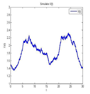
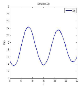
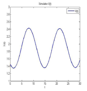
Figure 1: From left to right: Graphs of $x^{\varepsilon,\delta}(t)$ of solutions to Eq. (6.1) with $(\varepsilon,\delta)=(0.01,0.01)$, $(\varepsilon,\delta)=(0.001,0.001)$ and $x(t)$ to the averaged Eq. (6.2) respectively.

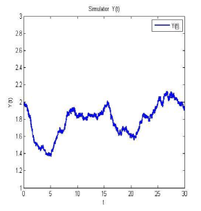
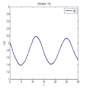
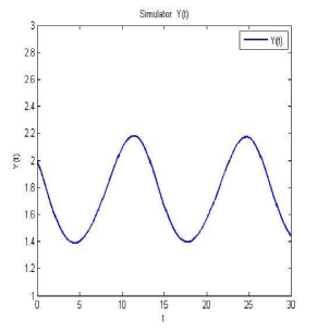
Figure 2: From left to right: Graphs of $y^{\varepsilon,\delta}(t)$ of solutions to Eq. (6.1) with $(\varepsilon,\delta)=(0.01,0.01)$, $(\varepsilon,\delta)=(0.001,0.001)$ and $y(t)$ to the averaged Eq. (6.2) respectively.

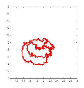
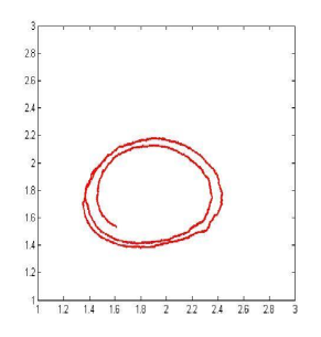
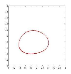
Figure 3: From left to right: Phase portraits of sample solutions to Eq. (6.1) with $(\varepsilon,\delta)=(0.01,0.01)$, $(\varepsilon,\delta)=(0.001,0.001)$ and to the averaged Eq. (6.2) respectively.

References

- [1] Bellet, L. R. Ergodic properties of Markov processes. In Open Quantum Systems II, Springer Berlin Heidelberg, (2006) 1-39.
- [2] N.H. Dang, N.H. Du, T.V. Ton, Asymptotic behavior of predator-prey systems perturbed by white noise, Acta Appl. Math. , 115(3) (2011), 351–370.
- [3] N.H. Du, D.H. Nguyen, and G. Yin, Conditions for permanence and ergodicity of certain stochastic predator-prey models, J. Appl. Probab. 53 (2016), no. 1, 187-202.
- [4] W. Fleming, Stochastically perturbed dynamical systems. Rocky Mountain J. Maths 4(1974), 407–433.
- [5] X. Han and P.E. Kloeden, Non-autonomous lattice systems with switching effects and delayed recovery, J. Differential Equations 261 (2016), 2986- 3009.
- [6] X. Han and H.N. Najm, Dynamical structures in stochastic chemical reaction systems, SIAM J. Appl. Dyn. Syst. 13 (2014), 1328- 1351.
- [7] Q. He and G. Yin, Large deviations for multi-scale Markovian switching systems with a small diffusion, Asymptotic Anal., 87 (2014) 123–145.
- [8] Q. He, G. Yin, Q. Zhang, Large deviations for two-time-scale systems driven by nonhomogeneous Markov chains and associated optimal control problems. SIAM J. Control Optim. 49 (2011), no. 4, 1737–1765.
- [9] C.J. Holland, Ergodic expansions in small noise problems, J. Differential Equations 16 (1974), 281–288.
- [10] C.J. Holland, Stochastically perturbed limit cycles. J. Appl. Probab. 15 (1978), no. 2, 311–320.
- [11] C. Ji, D. Jiang, Dynamics of a stochastic density dependent predator-prey system with Beddington-DeAngelis functional response. J. Math. Anal. Appl, 381 (2011), 441–453.
- [12] C. Ji, D. Jiang, and N. Shi, A note on a predator-prey model with modified Leslie-Gower and Hollingtype II schemes with stochastic perturbation, J. Math. Anal. Appl. 377 (2011), 435–440.
- [13] D. Liu, Analysis of multiscale methods for stochastic dynamical systems with multiple time scales, Multiscale Model. Simul. 8 (2010), 944- 964.
- [14] X. Mao, Stochastic Differential Equations and Applications (2007), Elsevier.
- [15] X. Mao, C. Yuan Stochastic differential equations with Markovian switching (2006), London: Imperial College Press.
- [16] S.P. Meyn and R.L. Tweedie, Stability of Markovian processes III: Foster-Lyapunov criteria for continuous-time processes, Adv. Appl. Prob. 25 (1993), 518–548.
- [17] D.H. Nguyen, G. Yin, Coexistence and exclusion of stochastic competitive Lotka-Volterra models, J. Differential Eqs. 262 (2017), no. 3, 1192-1225.
- [18] S.P. Sethi and Q. Zhang, Hierarchical Decision Making in Stochastic Manufacturing Systems, Birkhäuser, Boston, MA, 1994.
- [19] A. Sikder, and A.B. Roy, Limit cycles in a prey-predator system, Appl. Math. Lett. 6 (1993), no. 3, 91–95.
- [20] H.A. Simon and A. Ando, Aggregation of variables in dynamic systems, Econometrica, 29 (1961), 111–138.
- [21] F. Wu nad S. Hu, Attraction, stability and robustness for stochastic functional differential equations with infinite delay, Automatica, 47 (2011), 2224- 2232.
- [22] G. Yin and C. Zhu, Hybrid Switching Diffusions: Properties and Applications, (2010), Springer.