Quantum to classical transitions in causal relations

Abstract

The landscape of causal relations that can hold among a set of systems in quantum theory is richer than in classical physics. In particular, a pair of time-ordered systems can be related as cause and effect or as the effects of a common cause, and each of these causal mechanisms can be coherent or not. Furthermore, one can combine these mechanisms in different ways: by probabilistically realizing either one or the other or by having both act simultaneously (termed a physical mixture). In the latter case, it is possible for the two mechanisms to be combined quantum-coherently. Previous work has shown how to experimentally realize one example of each class of possible causal relations. Here, we make a theoretical and experimental study of the transitions between these classes. In particular, for each of the two distinct types of coherence that can exist in mixtures of common-cause and cause-effect relations—coherence in the individual causal pathways and coherence in the way the causal relations are combined—we determine how it degrades under noise and we confirm these expectations in a quantum-optical experiment.

I Introduction

The study of quantum correlations that arise from entangled particles has played an important role in the advancement of quantum physics and the development of quantum technologies O’Brien et al. (2009). As such, the loss of coherence has been extensively studied in quantum information, from quantum error correction Bennett et al. (1996) to the investigation of the loss of entanglement Yu and Eberly (2009), and also as a way to probe the quantum-classical boundary Zurek (2003); Raimond et al. (2001). Causal relations are a powerful way of structuring our understanding of complex systems Pearl (2000); Spirtes et al. (2000) and a more complete picture of any theory requires an understanding of the possible causal relations. Yet the interplay between causality and quantum theory gives rise to long-standing puzzles: famously, Bell inequality violations show that quantum mechanics is not compatible with the conventional account of causation Wood and Spekkens (2015). At the same time, novel types of causal relations that can only hold between quantum systems have been shown to provide advantages in computing and information processing Hardy (2007); Chiribella (2012); Araújo et al. (2014); Procopio et al. (2015); Ried et al. (2015). However, the effect of decoherence on these nonclassical causal relations has not yet been explored. Assessing how robust non-classical causal relations are against decoherence and experimental noise is thus a necessary step before exploiting them as a resource in quantum information processing.

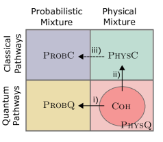
Figure 1: Classes of causal relations. A causal relation that is either cause-effect, common-cause, or a combination of both can be classified according to two criteria. The more familiar question is whether the mechanisms that realize the common-cause and cause-effect relations are themselves classical (C) or quantum (Q) that is, whether the common cause produces separable or entangled states and whether the cause-effect relation is a coherence-breaking or coherence-preserving channel. Another distinction is whether the two mechanisms are combined in a probabilistic mixture (Prob), a physical mixture (Phys), or in a way that is intrinsically quantum (Coh). (Formal definitions are provided in the text.) These distinctions give rise to five categories of interest, as shown above. (i)-(iii) Our experiment explores the transition from the most restrictive category, Coh, to ProbQ and PhysC (solid arrows), as well as the classical transition from PhysC to ProbC (dashed arrow).

Another critical task in the development of quantum causality is the systematic classification of the possible causal relations between quantum systems. We consider this problem in the case of two time-ordered quantum systems, where the possibilities are: a cause-effect relation, an unobserved common cause, or any combination of the two. For such scenarios, we have previously proposed a classification of the possible causal relations, shown in Fig. 1, which is based on two distinctions: whether the individual pathways (cause-effect or common-cause) are quantum or classical and whether they are combined probabilistically or in a more general way, termed a physical mixture. In Ref. MacLean et al. (2016), we investigated and experimentally realized particular examples of each class, including a fundamentally distinct type: a quantum-coherent mixture of cause-effect and common-cause relations.

We now turn our attention to the transitions between these classes, in particular, the transitions that are induced by decoherence. We explore the transition from fully quantum-coherent mixtures of common-cause and cause-effect relations (Coh) to two other types of mixtures: a probabilistic mixture of common-cause and cause-effect mechanisms wherein each mechanism exhibits quantum coherence (ProbQ) and a physical mixture wherein both mechanisms are incoherent (PhysC).

These scenarios, which can only be represented using an extension of the standard quantum formalism, such as is provided in Refs. Aharonov et al. (2009); Leifer (2006); Chiribella et al. (2009); Hardy (2012); Silva et al. (2014); Oreshkov et al. (2012); Fitzsimons et al. (2013) and in particular Refs. Ried et al. (2015); MacLean et al. (2016), exemplify the loss of two different types of coherence: on the one hand, decoherence in the individual mechanisms, and on the other, decoherence in the way the causal mechanisms are combined. The latter is a type of quantum-to-classical transition that has not been previously considered. Moreover, by ranging over different families of causal maps instead of just isolated examples, we put the theoretical framework of Refs. Leifer and Spekkens (2013); Ried et al. (2015); MacLean et al. (2016) to a more stringent test.

II Causal relations between two quantum systems

The most general causal relation between two time-ordered quantum systems can be realized by the circuit fragment shown in Fig. 2. Its functionality, that is, the causal relation, is completely characterized by a trace-preserving, completely positive map from the input of the circuit fragment, labeled $D$, to the two outputs, $B$ and $C$: $\mathcal{E}_{CB|D}:\mathcal{L}(\mathcal{H}_{D})\rightarrow\mathcal{L}(\mathcal{H}_{CB})$, Ried et al. (2015); Chiribella et al. (2009); Hardy (2012); Oreshkov et al. (2012); Silva et al. (2014), and which we call the causal map.

We here adopt the classification of causal maps proposed in Ref. MacLean et al. (2016), which we review presently. A causal map descibes a purely cause-effect relation if it reduces to the form $\mathcal{E}_{CB|D}=\mathcal{E}_{B|D}\otimes\rho_{C}$ and a purely common-cause relation if it takes the form $\mathcal{E}_{CB|D}=\rho_{CB}{\rm Tr}_{D}$. A causal map $\mathcal{E}_{CB|D}$ is said to encode a probabilistic mixture of cause-effect and common-cause relations if it can be realized as follows: there is a hidden classical control variable, $J$, which only influences $B$, such that for every value of $J$, either $B$ depends only on $D$ or $B$ depends only on its common cause with $C$. (See the Supplemental Information of Ref. MacLean et al. (2016) for a discussion of why this definition is apt.) Any causal map that cannot be cast in this form is termed a physical mixture.

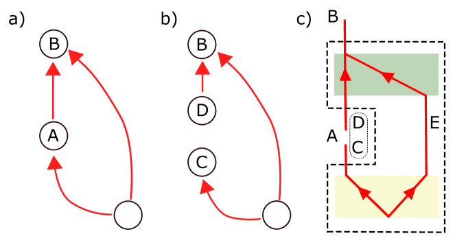
Figure 2: General causal relation between two quantum systems. (a) When the causal relations are represented as a directed acyclic graph, with arrows representing causal influences, one can distinguish the cause-effect pathway and the common-cause pathway. (b) In order to fully characterize the general causal relation between $A$ and $B$, the single system $A$ is replaced by two distinct systems: $C$ shares a common-cause relation with $B$, and $D$ has a cause-effect relation to $B$. (c) The general causal relation between $A$ and $B$ is realized by the circuit fragment inside the dashed box, with $C$ and $D$ representing an output and input, respectively. The label $E$ denotes the system that mediates the influence of the common cause on $B$.

The first criterion for classifying causal relations is whether they are quantum-coherent in the common-cause pathway (which relates $B$ to $C$) and in the cause-effect pathway (relating $B$ to $D$). A causal map is said to exhibit quantumness in the common-cause pathway if and only if there exists an orthogonal basis of pure states on $D$, labeled by $d$ and denoted $\{\Pi_{D}^{d}\}$, such that preparing each of these states generates a state on $C$ and $B$, $\tau_{CB}^{d}\equiv\mathcal{E}_{CB|D}(\Pi_{D}^{d})$, which is entangled. The definition of quantumness in the cause-effect pathway is closely analogous: given a measurement on $C$, it assesses whether the correlations between $B$ and $D$ that arise for each measurement outcome on $C$ exhibit entanglement. A state $\tau_{BD}^{c}$ that encodes these correlations can be constructed as follows: let $\Pi_{C}^{c}$ denote the operator associated with a measurement outcome $c$, let $\tau_{CBD}$ denote the state that is Choi isomorphic Choi (1975) to $\mathcal{E}_{CB|D}$, and take $\tau_{BD}^{c}\equiv\frac{1}{P(c)}{\rm Tr}_{C}\left(\Pi^{c}_{C}\tau_{CBD}\right)$, where $P(c)={\rm Tr}\left(\Pi^{c}_{C}\tau_{CBD}\right)$ ensures unit trace. A causal map is quantum in the cause-effect pathway if and only if there exists a rank-one projective measurement on $C$ such that, for all outcomes $c$, the states $\tau_{BD}^{c}$ are entangled. In order to quantify the entanglement in the induced states of the form $\tau^{z}_{XY}$, we compute their negativity Vidal and Werner (2002),

$$\mathcal{N}^{z}_{XY}\equiv\frac{1}{2}({\rm Tr}|T_{Y}(\tau^{z}_{XY})|-1),$$ (1)

where $T_{Y}(\cdot)$ denotes transposition on $Y$.

The second criterion for classifying causal relations is whether the common-cause and cause-effect mechanisms are combined as a probabilistic mixture or as a physical mixture. A special instance of the latter class is a quantum-coherent mixture (the definition of which will be provided momentarily). In order to formalize and detect these distinctions, we note the following: if $B$ was either purely cause-effect related to $D$ or purely common-cause related to $C$, then acquiring new information about $B$ either leads one to update one’s information about $D$ or it leads one to update one’s information about $C$, respectively, but it does not give rise to correlations between $C$ and $D$. If such correlations are observed, then, they herald a mixture of common-cause and cause-effect mechanisms. Moreover the strength of the induced correlations can distinguish between probabilistic and physical mixtures  MacLean et al. (2016).

In order to assess these correlations, we define an induced state $\tau_{CD}^{b}$ similarly to $\tau_{BD}^{c}$ above: given a measurement on $B$ with outcomes $b$ associated with operators $\Pi^{b}$, let $\tau_{CD}^{b}\equiv\frac{1}{P(b)}{\rm Tr}_{B}\left(\Pi^{b}_{B}\tau_{CBD}\right)$. [The normalization factor $P(b)$ is the probability of obtaining outcome $b$ if one inputs the maximally mixed state on $D$ into the causal map.] We apply two metrics to the induced state.

In the first, we test whether two qubits are related by a probabilistic mixture of common-cause and cause-effect mechanisms. We consider a measurement of $\sigma_{z}$ on $B$, whose outcomes we label $b=\pm 1$, introduce the covariance of the outcomes of Pauli measurements in state $\tau_{CD}^{b}$,

$${\rm cov}\left(\tau_{CD}^{b}\right)\equiv \langle\sigma^{x}_{C}\otimes\sigma^{y}_{D}\rangle-\langle\sigma^{x}_{C}\rangle\langle\sigma^{y}_{D}\rangle$$ (2)

and define the witness

$$\mathcal{C}_{CD}\equiv 2\sum_{b=\pm 1}bP(b)^{2}{\rm cov}(\tau_{CD}^{b}).$$ (3)

It was shown in Ref. MacLean et al. (2016) that $\mathcal{C}_{CD}=0$ for all probabilistic mixtures, hence non-zero values herald physical mixtures.

The second metric tests whether the cause-effect and common-cause mechanisms are combined coherently. If there exists a rank-one projective measurement on $B$ such that the states $\tau_{CD}^{b}$ are entangled for all possible outcomes $b$, then the causal map is said to exhibit a quantum Berkson effect: a quantum version of Berkson’s effect, whereby conditioning on a variable induces correlations between its causal parents which are otherwise uncorrelated. Again, we quantify this in terms of negativity, Eq. (1). Following the proposal of Ref. MacLean et al. (2016), a causal map is termed a quantum-coherent mixture of common-cause and cause-effect mechanisms if and only if (a) it exhibits a quantum Berkson effect and (b) it is not entanglement breaking in both the common-cause and cause-effect pathways.

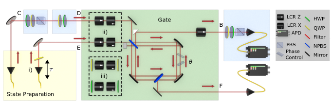
Figure 3: Optical implementation for exploring causal relations. The initial preparation (yellow) targets the maximally entangled state $\left|\Phi^{+}\right>$ from Eq. (4). The gate (green) allows the implementation of different ways of combining a common-cause relation (between $C$ and $B$) with a cause-effect relation (between $D$ and $B$). Measurements of $C$ and $B$ and repreparations of $D$ (blue) are used to characterize the causal relation. We explore the transitions (i) Coh to ProbQ, where we fix the dephasing probability ($p=0$) and phase ($\theta=\pi/2$) and vary the delay $\tau$ of the photon at $E$; (ii) Coh to PhysC, where we fix the dephasing directions along $(\hat{x},\hat{y},\hat{z})$ and vary the phase $\theta$ (by tilting the glass plates in the interferometer) and the dephasing probability $p$ (by switching the LCRs on with probability $p$); (iii) PhysC to ProbC, where we fix the dephasing probability ($p=1$) and phase ($\theta=\pi/2$) while interpolating from $(\hat{n}_{E},\hat{n}_{D},\hat{n}_{B})=(\hat{z},\hat{z},\hat{z})$ to $(\hat{x},\hat{y},\hat{z})$ using a single-parameter family of gates (see Eq. 10). Notation for optical elements: half-wave plate (HWP), quarter-wave plate (QWP), liquid-crystal retarder (LCR), polarizing beam splitter (PBS), non-polarizing beam splitter (NPBS), avalanche photo diode (APD).

III Realizing families of causal maps

In Ref. MacLean et al. (2016), we used a circuit similar to Fig. 3 in order to realize four particular causal maps that constitute paradigmatic examples of the classes introduced in Fig. 1. Here we introduce a modified set-up in order to observe the transitions shown in Fig. 1: Coh to ProbQ, Coh to PhysC, and PhysC to ProbC.

The initial state $\rho_{CE}$ in all cases is the maximally entangled state

$$\left|\Phi^{+}\right>\equiv\frac{1}{\sqrt{2}}(\left|HH\right>+\left|VV\right>),$$ (4)

where $\left|H\right>$, $\left|V\right>$ denote respectively the horizontal and vertical polarization states. The entanglement in the initial state provides the common cause relation in the experiment and can be removed with full dephasing noise. Between $DE$ and $BF$ we apply the partial swap gate, which realizes a family of unitaries parametrized by the parameter $\theta$,

$$\begin{split}U_{BF|DE}=\cos\frac{\theta}{2}\mathds{1}_{B|D}\otimes\mathds{1}_{F|E}+i\sin\frac{\theta}{2}\mathds{1}_{B|E}\otimes\mathds{1}_{F|D},\end{split}$$ (5)

where $\mathds{1}_{Y|X}$ denotes the identity operator with input space $X$ and output space $Y$. When $\theta=0$, the unitary reduces to the two-qubit identity operator, whereas when $\theta=\pi$, it reduces to the swap operator. When $\theta=\pi/2$, this gate reduces to the square root of swap or partial swap operator C̆ernoch et al. (2008); MacLean et al. (2016). When this partial swap gate is combined with the initial state on $CE$ described above, it was shown in Ref. MacLean et al. (2016) that it realizes our paradigm example of Coh: a causal map that is quantum in the common-cause and cause-effect pathways and furthermore exhibits a quantum Berkson effect.

We first study a transition from our example of Coh to an example of ProbQ, a causal map that is a probabilistic mixture of common-cause and cause-effect relations, which are individually quantum. To realize this transition, we introduce a delay $\tau$ between the two photons entering the interferometer. In Ref. MacLean et al. (2016), it was shown that the causal map went from Coh to ProbQ as the delay $\tau$ was increased beyond the coherence length $\tau_{coh}$ of the photons. We can exploit this to follow the evolution across this transition for intermediate values of $\tau$. The gate is then modelled as

$$\begin{split}\mathcal{E}_{BF|DE}&(\cdot)=qU_{BF|DE}(\cdot)U_{BF|DE}^{\dagger}\\ &+(1-q)\Big{[}\tfrac{1}{2}\mathds{1}_{B|D}\otimes\mathds{1}_{F|E}(\cdot)\mathds{1}_{B|D}\otimes\mathds{1}_{F|E}\\ &\hskip 36.98866pt+\tfrac{1}{2}\mathds{1}_{B|E}\otimes\mathds{1}_{F|D}(\cdot)\mathds{1}_{B|E}\otimes\mathds{1}_{F|D}\Big{]},\end{split}$$ (6)

where the factor $q=\exp(\tau^{2}/2\tau_{coh}^{2})$ expresses the amount of temporal overlap between two pulses, as a function of the delay $\tau$ between them, assuming two Gaussian pulses with a (RMS) coherence length of $\tau_{coh}$. Starting from our example of Coh ($q=1$), as the delay increases, the overlap of the photons decreases and we realize our paradigm example of ProbQ when $q=0$.

For the second transition, we apply dephasing channels on $D$, $E$ and $B$. The generic single-qubit dephasing channel is specified by the basis in which the dephasing occurs, represented by a Bloch vector $\hat{n}$, and the dephasing probability, denoted $p$:

$$\Delta(\hat{n},p)(\rho)\equiv(1-p/2)\rho+p/2\left([\hat{n}\cdot\vec{\sigma}]\rho[\hat{n}\cdot\vec{\sigma}]\right).$$ (7)

Complete dephasing ($p=1$) along $\hat{y}$ on $D$, $\hat{x}$ on $E$ and $\hat{z}$ on $B$ realizes our paradigm example of PhysC. In this case, the gate is

$$\mathcal{E}_{BF|DE}(\cdot)\equiv$$ (8)

$$(\Delta^{B}(\hat{z},1)\otimes\mathcal{I}_{F})\left(U_{BF|DE}\left\{[\Delta^{D}(\hat{y},1)\otimes\Delta^{E}(\hat{x},1)](\cdot)\right\}U_{BF|DE}^{{\dagger}}\right),$$

where $\mathcal{I}_{F}$ is the identity map on $F$. The transition from Coh to PhysC is then realized by fixing the direction of dephasing ($\hat{y}$ on $D$, $\hat{x}$ on $E$ and $\hat{z}$ on $B$) but ranging over the dephasing probability, $p$.

Finally, note that complete dephasing ($p=1$) along $\hat{z}$ on each of $D$, $E$ and $B$ generates our paradigm example of ProbC. Here, the gate is

$$\mathcal{E}_{BF|DE}(\cdot)\equiv$$ (9)

$$(\Delta^{B}(\hat{z},1)\otimes\mathcal{I}_{F})\left(U_{BF|DE}\left\{[\Delta^{D}(\hat{z},1)\otimes\Delta^{E}(\hat{z},1)](\cdot)\right\}U_{BF|DE}^{{\dagger}}\right).$$

We can therefore realize a one-parameter family of causal maps that interpolate between our paradigm examples of PhysC and ProbC by rotating the bases in which $D$, $E$, and $B$ are dephased. The directions along which each of these systems is dephased, with full dephasing strength ($p=1$), is parameterized by $\eta$, and given as:

$$\begin{split}\hat{n}_{E}=&\cos{2\eta}~{}\hat{x}+\sin{2\eta}~{}\hat{z},\\ \hat{n}_{D}=&\cos{2\eta}\sin 2\eta~{}\hat{x}-\cos 2\eta~{}\hat{y}+\sin^{2}{2\eta}~{}\hat{z},\\ \hat{n}_{B}=&\hat{z}.\end{split}$$ (10)

As one varies between $\eta=0$ and $\eta=\pi/4$, one transitions between full dephasing along the triple of axes $(\hat{n}_{E},\hat{n}_{D},\hat{n}_{B})=(\hat{x},\hat{y},\hat{z})$ to full dephasing along the triple of axes $(\hat{z},\hat{z},\hat{z})$ and hence between our paradigm examples of PhysC and of ProbC.

IV Experiment

The experimental set-up is shown in Fig. 3. We aim to produce polarization-entangled photons at 790 nm in the state $\left|\Phi^{+}\right>$. The polarization of one photon is measured at $C$ using a half-wave plate (HWP), quarter-wave plate (QWP), and polarizing beam splitter (PBS) in sequence, after which the photon is reprepared in another polarization state at $D$. At $D$ and $E$, both photons are then sent towards the quantum circuit, which uses a folded displaced Sagnac interferometer MacLean et al. (2016), with two 50/50 beam splitters and two NBK-7 glass windows that are counter rotated in order to change the phase $\theta$ with minimal beam deflection. The polarization of the photon at $B$ is measured and detected in coincidence with the one at $F$. The photon (RMS) coherence length, $\tau_{coh}=189$ fs, is estimated using a Hong-Ou Mandel interference measurement at the first beam splitter assuming transform-limited Gaussian pulses.

The implementation of the partial swap $U_{BF|DE}$ of Eq. (5) in an optical circuit follows C̆ernoch et al. (2008); MacLean et al. (2016). When two indistinguishable photons arrive at the first beam splitter, they will bunch if their polarization state lies in the symmetric subspace, and they will anti-bunch if their polarization state lies in the anti-symmetric subspace. If they bunch, only the clockwise path in Fig. 3, which introduces no phase shift, can lead to a coincidence at $B$ and $F$. However, if they anti-bunch, the photon that travels along the counter-clockwise path will acquire an extra phase $\theta$, while the other, on the clockwise path, acquires no extra phase. Since the photons are indistinguishable, these two paths are coherently recombined and as a result the gate applies a phase difference $\theta$ between the symmetric and anti-symmetric projections of the photon state, leading to the partial swap unitary of Eq. (5). Further details on the single photon source and Sagnac interferometer are provided in Ref. MacLean et al. (2016).

The dephasing channels before and after the Sagnac interferometer are implemented using variable liquid crystal retarders (LCR), which apply a voltage-dependent birefringence, introducing a phase shift of $0$ or $\pi$. Each axis for dephasing can be chosen independently. Dephasing along the $\hat{z}$ direction of the Bloch sphere is achieved by putting the LCR axis at $0^{\circ}$, dephasing along the $\hat{x}$ direction, by putting the LCR at $45^{\circ}$, and in the $\hat{y}$ direction, by simultaneously switching on two LCRs, one at $0^{\circ}$ and one at $45^{\circ}$. Dephasing in the rotated basis is achieved by setting two QWPs on either side of an LCR at $0^{\circ}$ and two HWPs on either side of an LCR at $45^{\circ}$. The transition from full dephasing along the triple of axes $(\hat{n}_{E},\hat{n}_{D},\hat{n}_{B})=(\hat{x},\hat{y},\hat{z})$ to full dephasing along the triple of axes $(\hat{z},\hat{z},\hat{z})$ that is described in Eq. (10) is therefore implemented with the following transformations on $E$, $D$, and $B$,

$$E:U_{\mathrm{HWP}}(\eta/2)\Delta(\hat{x},p=1)U_{\mathrm{HWP}}(\eta/2)$$

$$D:U_{\mathrm{QWP}}(3/4\pi-\eta)\Delta(\hat{z},p=1)U_{\mathrm{QWP}}(\pi/4-\eta)$$

$$B:\Delta(\hat{z},p=1),$$

where $U_{\mathrm{HWP}}(\eta)$ and $U_{\mathrm{QWP}}(\eta)$ specify the unitaries for a HWP and QWP, respectively, with the fast axis at an angle $\eta$, while $\Delta(\hat{x},p=1)$ and $\Delta(\hat{z},p=1)$ are the completely dephasing channels implemented with LCRs.

V Results

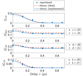
Figure 4: Transition from Coh to ProbQ. As the delay $\tau$ between photons is increased, quantum interference at the gate is gradually lost. We observe: (a) the witness of physical mixture $\mathcal{C}_{CD}$; (b) the negativity $\mathcal{N}_{BD}$ under post-selection on eigenstates of $\sigma_{X}$ on $C$; (c) the negativity $\mathcal{N}_{CB}$ under pre-selection on eigenstates of $\sigma_{Y}$ on $D$; and (d) the negativity $\mathcal{N}_{CD}$ under post-selection on eigenstates of $\sigma_{Z}$ on $B$. (b),(c) Nonzero values of $\mathcal{N}_{BD}$ and $\mathcal{N}_{CB}$ herald quantumness in the common-cause and cause-effect pathways, which is preserved throughout the transition, while (a),(d) the quantum Berkson effect is supressed before the witness of physical mixture reaches zero. For intermediate values, between $\tau=0.27$ ps ($q=0.23$) and $\tau=0.39$ ps ($q=0.05$), we realize a causal map that belongs to PhysQ, but observe no evidence that it belongs to Coh. For larger delays, there is no evidence of physical mixture ($\mathcal{C}_{CD}=0$), making the data consistent with ProbQ. Solid lines represent theoretical predictions in the ideal case (red) and taking into account the experimental implementation (blue), as described in the text.

In Fig. 4, we observe signatures of the transition from Coh to ProbQ, which is generated by delaying one photon relative to the other before the gate. The indicators of quantumness in the common-cause and cause-effect pathways, $\mathcal{N}_{CB}$ and $\mathcal{N}_{BD}$, remain non-zero throughout the transition, whereas the witnesses of physical mixture, $\mathcal{C}_{CD}$, and of the quantum Berkson effect, $\mathcal{N}_{CD}$, fall to zero as the delay increases, since the photons become distinguishable and coherence in the gate is lost. Thus, although the individual common-cause and cause-effect mechanisms remain quantum, we observe a loss of coherence in the way in which they are combined. This exemplifies the transition from Coh to ProbQ.

Comparing Figs. 4(a) and 4(d), the indicator of a coherent mixture falls more quickly than the indicator of physical mixture, giving rise to a range of values of the delay parameter for which the causal map is still a physical mixture of quantum common-cause and cause-effect mechanisms (PhysQ) but $\mathcal{N}^{b}_{CD}$ is zero for both $\left|H\right>$ and $\left|V\right>$ on $B$. For the family of causal maps that we target in this transition, the measurement $\{\left|H\right>,\left|V\right>\}$ on $B$ maximizes the induced negativity, and consequently finding $\mathcal{N}^{b}_{CD}=0\;\forall b=H,V$ suggests that no measurement could have induced entanglement. In this case, the causal map is an element of PhysQ, but not of Coh.

The indicators we observe are generally degraded by imperfections in the state preparation and the partial swap gate. In order to take these into account in the theoretical predictions, we use the tomographic reconstruction of the causal map MacLean et al. (2016) in the scenario with no delay to predict the witness values when $\tau$ is non-zero, yielding the blue curves in Fig. 4. Similar derivations are used for the blue lines in Figs. 5 and 6, starting from the case with no dephasing to generate predictions for arbitrary $p$ and $\eta$.

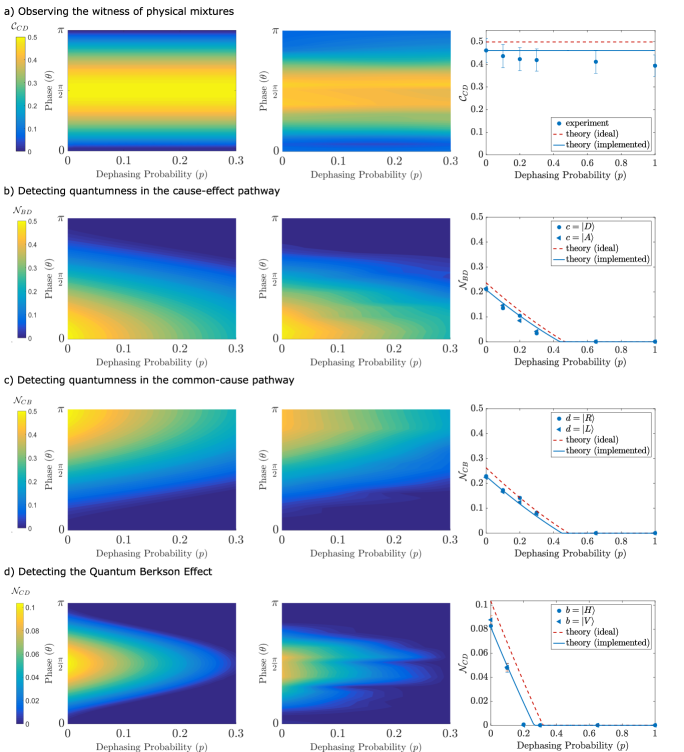
Figure 5: Classifying a family of causal relations: transition from Coh to PhysC. (a) Witness of physical mixture $\mathcal{C}_{CD}$, (b) negativity $\mathcal{N}_{BD}$ for measurements of $\sigma_{X}$ eigenstates on $C$, (c) negativity $\mathcal{N}_{CB}$ for preparations of $\sigma_{Y}$ eigenstates on $D$, and (d) negativity $\mathcal{N}_{CD}$ for measurements of $\sigma_{Z}$ eigenstates on $B$. For each witness, we present: (left) theoretical predictions, which are identical for selection on either eigenstate; (middle) experimental data under selection on the $+1$ eigenstate; (right) a two-dimensional cross section through the contour plot at $\theta=92.8^{\circ}$, comparing experimental data for both selections (blue circles and triangles) with theoretical expectations assuming no experimental imperfections (red curve) and with theoretical expectations given an estimate of the experimental imperfections inferred from the tomographically-reconstructed causal map realized at $p=0$ (blue curve). We observe: (a) The witness of physical mixture remains constant throughout the transition. (b)–(d) Quantumness in the common-cause and cause-effect pathways persists longer than quantumness in the way that the two mechanisms are combined. As we range from purely common-cause ($\theta=\pi$) to purely cause-effect ($\theta=0$), the signature of coherence in the cause-effect pathway increases, whereas the signature of coherence in the common-cause pathway diminishes.

The transition from Coh to PhysC is shown in Fig. 5. The vertical axis denotes the experimentally-implemented value of the parameter $\theta$ in the family of partial swap unitaries described in Eq. (5). This ranges from $\theta=0$ (purely cause-effect) to $\theta=\pi$ (purely common-cause) through a family of intrinsically quantum combinations of the two. The value of $\theta$ that is realized by the interferometer is estimated by fitting our experimental data to a family of causal maps where $\theta$ is the only free parameter. The horizontal axis denotes the values of the dephasing probability $p$ common to the three dephasing operations along the fixed axes $(\hat{n}_{E},\hat{n}_{D},\hat{n}_{B})=(\hat{x},\hat{y},\hat{z})$. The dephasing probability $p$ ranges from $0$ (intrinsically quantum) to $1$ (classical), although we display only the interesting region below $p=0.3$.

Figure 5(a) depicts the value of $\mathcal{C}_{CD}$ from Eq. (3), which witnesses the presence of a physical mixture. Figures 5(b)-5(d) show the value of the negativities [defined in Eq. (1)] for certain bipartite states. Figure 5(b) displays $\mathcal{N}^{c}_{BD}$, the negativity of the state on $BD$ inferred from obtaining the $c$ outcome in a measurement of $\sigma_{X}$ on $C$. Figure 5(c) displays $\mathcal{N}^{d}_{CB}$, the negativity of the state on $CB$ that results from the preparation of the $d$ eigenstate of $\sigma_{Y}$ on $D$. Figure 5(d) displays $\mathcal{N}^{b}_{CD}$, the negativity of the state on $CD$ inferred from obtaining the $b$ outcome in a measurement of $\sigma_{Z}$ on $B$. The first two [Figs. 5(b)-5(c)] detect the presence of coherence in the cause-effect and common-cause pathways, respectively, while the third Fig. 5(d) detects the quantum Berkson effect. For each witness, we compare the theoretical predictions (left panel) with the experimental data (middle column). For the negativities [Fig. 5(b)–5(d)], we only show data obtained from preselection and postselection of the +1 eigenstate; the theoretical predictions are the same for both eigenstates.

When there is no dephasing ($p=0$), as we vary the phase from a purely common-cause ($\theta=0$) to a purely cause-effect ($\theta=\pi$) relation, we observe that the witness $\mathcal{C}_{CD}$ [Fig. 5(a)] is non-zero, indicating that we continue to realize a physical mixture, for all but $\theta=0,\pi$ (purely cause-effect and common-cause). The witness $\mathcal{N}_{BD}$ [Fig. 5(b)] increases from zero and reaches a maximum at a purely cause-effect relation ($\theta=0$), whereas the witness $\mathcal{N}_{CB}$ [Fig. 5(c)] decreases to zero from a maximum at a purely common-cause relation ($\theta=\pi$). Finally, $\mathcal{N}_{CD}$ [Fig. 5(d)] reaches a maximum for an equally weighted coherent mixture of cause-effect and common-cause ($\theta=\pi/2$). This behavior is precisely what one expects theoretically for a family of causal maps, which coherently interpolate between cause-effect and common-cause relations.

The dephasing bases were chosen so as to ensure that the witness of physical mixture remains unaffected by the dephasing. This is possible because $\mathcal{C}_{CD}$ is evaluated using measurements in a single basis on each system, which implies that dephasing in this set of bases leaves all relevant measurement outcomes unchanged. As such, when the probability of dephasing, $p$, is increased, $\mathcal{C}_{CD}$ remains constant, whereas all other witnesses are decreased.

When the gate produces a purely cause-effect relation ($\theta=0$) and there is no dephasing ($p=0$), $\mathcal{N}_{BD}$ is found to be nonzero, heralding quantumness in the cause-effect pathway. As the phase or the dephasing is increased, i.e., as $\theta\rightarrow\pi$ or $p\rightarrow 1$, the value of the witness decreases until quantumness is no longer detected. Likewise, $\mathcal{N}_{CB}$ detects quantumness in the common-cause pathway when the gate produces a purely common-cause relation ($\theta=\pi$) and there is no dephasing ($p=1$). As the phase is decreased or the dephasing increased, i.e., as $\theta\rightarrow 0$ or $p\rightarrow 1$, the value of the witness decreases until no signature of quantumness in the common-cause pathway is left. Finally, the witness $\mathcal{N}_{CD}$ reveals signatures of the quantum Berkson effect when $p=0$ except near the extremes $\theta=0,\pi$. However, as the dephasing is increased towards $p=1$, these signatures vanish rapidly.

In the regions of the parameter space where all witnesses are nonzero, the experiment realizes a member of the class Coh, a quantum-coherent mixture of common-cause and cause-effect relations.

The right panel in Fig. 5 shows two-dimensional cross-sections at $\theta=92.8^{\circ}$. Comparing Fig.5(d) to Figs.5(b) and 5(c), we note that, as the dephasing increases, quantumness in the two pathways (revealed by $\mathcal{N}_{CB}\neq 0$ and $\mathcal{N}_{BD}\neq 0$) persists for longer than the quantum Berkson effect (the signature of which is $\mathcal{N}_{CD}\neq 0$). For the family of causal maps that we target, measuring $B$ in the $\{\left|H\right>,\left|V\right>\}$ basis induces the most entanglement, and as such, when $\mathcal{N}^{b}_{CD}=0\;\forall b\in\{H,V\}$, the causal map is no longer in Coh. Thus, we first observe a loss of coherence in the way the different causal pathways are combined, while remaining a physical mixture: a transition from Coh to PhysQ. This is followed by a gradual loss of coherence in the cause-effect and common-cause pathways, leading towards the class PhysC.

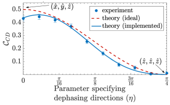
Figure 6: Transition from PhysC to ProbC. A nonzero value of the witness $\mathcal{C}_{CD}$ heralds a physical mixture of causal structures. The witness is evaluated for different dephasing directions parametrized by Eq. 10, with the extremes, $\eta=0$ and $\eta=\pi/4$, corresponding to settings for our examples of PhysC and ProbC, respectively. For $\eta=\pi/4$, we measure $\mathcal{C}_{CD}=0.01\pm 0.02$, which is compatible with a probabilistic mixture, whereas $\eta=0$ produces $\mathcal{C}_{CD}=0.44\pm 0.02$, demonstrating with high confidence a non-trivial physical mixture of cause-effect and common-cause mechanisms. The solid lines indicate theoretical predictions assuming no experimental imperfections (red) and assuming the intial experimental implementation and dephasing operation inferred by comparing the causal maps with and without dephasing (blue).

Finally, we explore the transition between PhysC and ProbC, which allows us to verify the sensitivity of the witness $\mathcal{C}_{CD}$. Figure 6 shows experimental points alongside the ideal theoretical curves (red) as well as theory curves based on the experimentally reconstructed causal map with no dephasing. The small discrepancy between the data and the ideal theory (red) is likely due to a slight rotation of the LCR at $C$. The effects of this rotation was measured by comparing the reconstructed causal maps for $\theta=\pi/2$ and $\eta=0$ with ($p=1$) and without ($p=0$) dephasing, and when accounted for, gives the adjusted theory curve (blue). The witness $\mathcal{C}_{CD}$ is clearly non-zero throughout most of the transition, thereby attesting to the existence of a physical mixture. The last two data points are within error of zero, with $\mathcal{C}_{CD}=0.01\pm 0.02$ when $\hat{n}_{D,E,B}=\hat{z}$ ($\eta=\pi/4$). This is consistent with the fact that only these values of dephasing in the system are compatible with a probabilistic mixture.

VI Conclusions

Starting from a causal map in the class Coh, a quantum-coherent mixture of cause-effect and common-cause mechanisms, we have experimentally observed both the transition to a causal map in the class ProbQ and the transition to a causal map in the class PhysC. Our results illustrate that general causal relations can exhibit two different types of coherence, which can vary independently. We observe coherence in pathways – that is, the quantum channel realizing a cause-effect relation and the bipartite state encoding a common-cause relation – which is gradually lost in the transition towards PhysC. We also observe coherence in the way that the two causal mechanisms are combined, that is, coherence in the mixture, which we gradually decrease in the transition towards ProbQ.

While the consequences of decoherence for entangled quantum states are well understood, for instance the loss of entanglement due to coupling to local independent environments Almeida et al. (2007), a theory of decoherence for quantum causal relations is more subtle. As shown here, it has an added level of richness due to the possibility of coherence not only in individual causal pathways, but in the way that these pathways are mixed. We find that in the presence of local environmental noise, the quantum to classical transition for the causal pathways, which corresponds to decoherence on a bipartite quantum state for the common-cause pathway and decoherence on a channel for the cause-effect pathway, is inherently different from the quantum to classical transition for the way in which the pathways are mixed. We have determined the amount of local noise that the individual pathways can tolerate before losing the quantumness present in their mixture, as measured by the quantum Berkson effect. Moreover, we observe that the coherence in the mixture is more sensitive to the type of noise presently studied, decaying faster than the coherence in the individual causal pathways.

The experimental exploration of the transition between quantum and classical causal relations is based on the formalism of causal maps and classes developed in Refs. Ried et al. (2015); MacLean et al. (2016), and is part of the larger program of advancing the causal understanding of quantum mechanics. In particular, to explore the novel types of causal relations that can hold in higher dimensions and among larger numbers of systems, it will be necessary to rely on different types of controlled noise as a tool for transitioning between various classes of causal relations.

References

- O’Brien et al. (2009) J. L. O’Brien, A. Furusawa, and J. Vuckovic, Nat. Photon 3, 687 (2009).
- Bennett et al. (1996) C. H. Bennett, D. P. DiVincenzo, J. A. Smolin, and W. K. Wootters, Physical Review A 54, 3824 (1996).
- Yu and Eberly (2009) T. Yu and J. H. Eberly, Science 323, 598 (2009).
- Zurek (2003) W. H. Zurek, in Quantum Decoherence, Progress in Mathematical Physics Vol 48 (Birkhauser Basel 2007) pp.1-31 .
- Raimond et al. (2001) J.-M. Raimond, M. Brune, and S. Haroche, Reviews of Modern Physics 73, 565 (2001).
- Pearl (2000) J. Pearl, Causality: Models, reasoning and inference (Cambridge University Press, New York, 2000).
- Spirtes et al. (2000) P. Spirtes, C. Glymour, and R. Scheines, Causation, prediction, and search (MIT Press, Cambridge, 2000).
- Wood and Spekkens (2015) C. J. Wood and R. W. Spekkens, New Journal of Physics 17, 033002 (2015).
- Hardy (2007) L. Hardy, “Quantum gravity computers: On the theory of computation with indefinite causal structure,” (2007).
- Chiribella (2012) G. Chiribella, Phys. Rev. A 86, 040301 (2012).
- Araújo et al. (2014) M. Araújo, F. Costa, and C. Brukner, Phys. Rev. Lett. 113, 250402 (2014).
- Procopio et al. (2015) L. M. Procopio, A. Moqanaki, M. Ara jo, F. Costa, I. A. Calafell, E. G. Dowd, D. R. Hamel, L. A. Rozema, C̆aslav Brukner, and P. Walther, Nat. Commun. 6, 7913 (2015).
- Ried et al. (2015) K. Ried, M. Agnew, L. Vermeyden, D. Janzing, R. W. Spekkens, and K. J. Resch, Nat. Phys. 11, 414 (2015).
- MacLean et al. (2016) J.-P. W. MacLean, K. Ried, R. W. Spekkens, and K. J. Resch, Nature Commun. 8, 1038 (2017).
- Aharonov et al. (2009) Y. Aharonov, S. Popescu, J. Tollaksen, and L. Vaidman, Phys. Rev. A 79, 052110 (2009).
- Leifer (2006) M. S. Leifer, Phys. Rev. A 74, 042310 (2006).
- Chiribella et al. (2009) G. Chiribella, G. M. D’Ariano, and P. Perinotti, Phys. Rev. A 80, 022339 (2009).
- Hardy (2012) L. Hardy, Philos. T. Roy. Soc. A 370, 3385 (2012).
- Silva et al. (2014) R. Silva, Y. Guryanova, N. Brunner, N. Linden, A. J. Short, and S. Popescu, Physical Review A 89, 012121 (2014).
- Oreshkov et al. (2012) O. Oreshkov, F. Costa, and C. Brukner, Nat. Commun. 3, 1092 (2012).
- Fitzsimons et al. (2013) J. Fitzsimons, J. Jones, and V. Vedral, Scientific Reports 5, 18281 (2015).
- Leifer and Spekkens (2013) M. S. Leifer and R. W. Spekkens, Phys. Rev. A 88, 052130 (2013).
- Choi (1975) M. D. Choi, Linear Algebra Appl. 10, 285 (1975).
- Vidal and Werner (2002) G. Vidal and R. F. Werner, Phys. Rev. A 65, 032314 (2002).
- C̆ernoch et al. (2008) A. C̆ernoch, J. Soubusta, L. Bartůšková, M. Dušek, and J. Fiurášek, Phys. Rev. Lett. 100, 180501 (2008).
- Almeida et al. (2007) M. P. Almeida, F. d. Melo, M. Hor-Meyll, A. Salles, S. P. Walborn, P. H. S. Ribeiro, and L. Davidovich, Science 316, 579 (2007).