Geometric Analysis of Observability of Target Object Shape Using Location-Unknown Distance Sensors

Abstract

We geometrically analyze the problem of estimating parameters related to the shape and size of a two-dimensional target object on the plane by using randomly distributed distance sensors whose locations are unknown. Based on the analysis using geometric probability, we discuss the observability of these parameters: which parameters we can estimate and what conditions are required to estimate them. For a convex target object, its size and perimeter length are observable, and other parameters are not observable. For a general polygon target object, convexity in addition to its size and perimeter length is observable. Parameters related to a concave vertex can be observable when some conditions are satisfied. We also propose a method for estimating the convexity of a target object and the perimeter length of the target object.

I Introduction

We investigate the problem of estimating parameters related to the shape and size of a target object by using randomly distributed distance sensors. An individual sensor in this paper is a simple sensor measuring the distance between a sensor and a target object. It is often composed of an infrared emitting diode and a position sensitive detector. Its output is the voltage corresponding to the distance. A typical example of this sensor is a commercial sensor produced by Sharp (Sharp GP2Y0A02YK0F), although it has no communication capability. In this paper, we assume that an individual sensor does not have a positioning function, such as a GPS, or functions for monitoring the target object size and shape, such as a camera, and it can be placed without careful design. However, the sensor has communication capability and sends reports. By collecting reports from individual sensors, we statistically estimate the parameters of target objects.

The fundamental questions for this problem under this paradigm are: Can we estimate the shape of the target object (or is its shape observable) under this paradigm? If yes, how can we estimate it? If no, what can we estimate? Nothing? This paper intends to answer these questions when distance sensors are used.

Although we also attempted to answer these questions in our prior studies [infocom, signalProcess, mobileComp, time-variant], we did not use distance sensors. By using binary sensors of a convex sensing area reporting on whether they detect a target object, size and perimeter length estimation was proven possible even when the locations of sensors were unknown. A size and perimeter length estimation method was proposed for use when the sensing area is convex [infocom]. To estimate additional parameters by using location-unknown sensors, combinations of binary sensors of a convex sensing area were proposed [signalProcess, mobileComp]. However, it is difficult to implement and deploy combined binary sensors called “composite sensor nodes”, particularly when the composite sensor nodes are large. Another extension was done [time-variant], where the target object was assumed to be time-variant.

As far as we know, there have been no other studies to directly tackle this question.

The main contribution of this paper is the development of a concept of observability of the target object shape when location-unknown distance sensors area used. For a convex target object, it has been proven that its size and perimeter length are observable parameters and that other parameters are non-observable. For a general target object, convexity is also observable and conditions under which some parameters related to concave vertices become observable are provided. We developed a method for estimating the size, perimeter length, and convexity of a target object by using distance sensors.

Unfortunately, some parameters are unobservable under the new sensing paradigm when the distance sensors are used. This means that this paradigm has some restrictions in target object shape estimation, while it works for some applications. For example, when we have a set of target object candidates and can distinguish them by their size, perimeter length, and convexity, this paradigm using the distance sensor can identify the target object. This paradigm is also appropriate in other applications such as forecasting or estimating thunder areas [time-variant], because the precise estimation of the thunder area is not needed but a rough shape such as its size or length is enough. Applications for roughly determining the environment before detailed monitoring are also suitable to this paradigm, particularly when a target object is moving. These applications can be used in an assistant robot to detect an object of interest in a search step.

II Model

There is a target object $T$ in a monitored area $\Omega\subset\mathbb{R}^{2}$. $T$ is a polygon, and its boundary $\partial T$ is closed and simple (no holes or double points) and consists of $n_{l}$ line segments. Let $l_{i}$ be the length of the $i$-th line segment and $\phi_{i}$ be the inner angle formed by the $i$-th and $(i+1)$-th (mod $n_{l}$) line segments (Fig. 1-(a)), where $i=1,\cdots,n_{l}$.

There are $n_{s}$ directional distance sensors deployed in $\Omega$. Each sensor has sensing capability to measure the distance to an object lying in the sensing direction within the maximum range $r_{max}$. Therefore, when the location of the sensor is ${\bf x}=(x,y)$ and its direction from the $x$-axis is $\theta$, the sensing range $S({\bf x},\theta)$ is $\{(x+s\cos\theta,y+s\sin\theta),0\leq\forall s\leq r_{max}\}$, and the measured distance $r$ to $T$ by this sensor is given as

$$\cases{\min_{(x+s\cos\theta,y+s\sin\theta)\in T}s,&for $S({\bf x},\theta)\cap T\neq\emptyset$,\cr\emptyset,&for $S({\bf x},\theta)\cap T=\emptyset$.}$$ (1)

In particular, $r=0$ if $(x,y)\in T$. Call the point $(x+r\cos\theta,y+r\sin\theta)$ as the detected point for a given $T$, ${\bf x}$, and $\theta$. Note that the detected point is on $\partial T$ if $r>0$ and in $T$ if $r=0$ and is unique.

These sensors are randomly deployed and their directions are also random and uniformly distributed in $[0,2\pi)$. For the $i$-th sensor ($i=1,\cdots,n_{s}$), let ${\bf x}_{i}$ be its location, $\theta_{i}$ be its direction, and $r_{i}$ be the measured distance to $T$. Assume that we do not know ${\bf x}_{i}$ or $\theta_{i}$ for any $i$. We may remove the subscript $i$ and use ${\bf x}$, $\theta$, and $r$ to simplify the notation. Because sensors monitor $\Omega$, assume that ${\bf x}_{i}\subset\Omega$ for all $i$. To remove the boundary effect of $\Omega$, assume that the location of $T$ satisfies $\{(x^{\prime},y^{\prime})|\sqrt{(a-x^{\prime})^{2}+(b-y^{\prime})^{2}}\leq r_{max},\forall(a,b)\subset T\}\subset\Omega$.

Each sensor can communicate with a server collecting sensing reports from individual sensors. It reports the measured distance $r$ between the sensor and $T$ if it detects within a range or reports “no detection” otherwise. Because it does not have a positioning function or a direction sensor, the report does not include ${\bf x}$ or $\theta$. All the sensors are assumed to send reports at each sensing epoch.

Although the target object and sensors can move, it is not necessary for us to assume their movement. This is because the analysis in this paper is based on the sensing results at each sensing epoch.

For a set $X\subset\mathbb{R}^{2}$, $|X|_{2}$ and $|X|_{1}$ denote its area size and perimeter length, respectively. In addition, for $X\subset\mathbb{R}^{2}\times[0,2\pi)$, $|X|_{3}\stackrel{{\scriptstyle\mathrm{def}}}{{=}}\int\!\!\!\int\!\!\!\int_{(x,y,\theta)\in X}dx\,dy\,d\theta$. Furthermore, ${\bf 1}(t)\stackrel{{\scriptstyle\mathrm{def}}}{{=}}\cases{1,&if $t$ is true,\cr 0,&otherwise,}$, $[t]^{+}\stackrel{{\scriptstyle\mathrm{def}}}{{=}}\cases{t,&if $t>0$,\cr 0,&otherwise,}$,

$\langle\sin(t)\rangle\stackrel{{\scriptstyle\mathrm{def}}}{{=}}\cases{|\sin(t)|,&if $3\pi/2<t<2\pi$,\cr 1,&if $\pi<t\leq 3\pi/2$,}$ and $\widehat{t}$ is an estimator of $t$.

Table I lists the variables and parameters used in the remainder of this paper for the reader’s convenience.

TABLE I: List of variables and parameters

$T$	target object
$\Omega$	monitored area
$l_{i}$	length of $i$-th line segment
$\phi_{i}$	inner angle formed by $i$-th and $(i+1)$-th
	line segments
$n_{s}$	number of sensors
$r_{max}$	maximum sensing range
${\bf x},\theta$	sensor’s location and direction
$r$	sample value of measured distance between sensor and $T$
$s$	variable describing measured distance between sensor and $T$
$T_{s}(r)$	$\{(x,y,\theta)|0<\min_{(x+s\cos\theta,y+s\sin\theta)\in T}s\leq r\}$
$\omega(r|\theta,l)$	region where sensor lies with $s\leq r$ and
	direction $\theta$ and sensor’s detected point is
	on line segment of length $l$
$v_{i}(r|\theta,l)$	overlap between $T$ and $\omega(r|\theta,l)$ for concave
	$\phi_{i}$
$N_{0}$	num. of sensing reports of which results are 0
$N_{+}$	num. of sensing reports of which results are positive
$N_{\emptyset}$	num. of sensing reports of which results are $\emptyset$
$N(r)$	num. of sensing reports of which results are
	less than $r$
$N(>r)$	$N_{+}-N(r)+N_{0}$
$N_{d}$	num. of sensing reports detecting $T$ ($=N_{0}+N_{+}$)
$e(r)$	$N(r)/n_{s}-\widehat{\Pr(s\leq r)}$
$\sigma$	(estimated) standard deviation of $e(r)$

III Integral geometry and geometric probability for our model

As a preliminary of the analysis in this paper, this section introduces a brief explanation on integral geometry and geometric probability available for our model.

A sensing area position is characterized by the sensor location $(x,y)$ and its direction $\theta$. We can define a probability that a set of sensing area positions satisfies a certain condition $X_{c}$. An example of $X_{c}$ is the sensing area position detecting the target $T$. When $(x,y)$ and $\theta$ are uniformly distributed, it is quite natural that this probability is given by the ratio of the size of the subspace $\{(x,y,\theta)|(x,y,\theta)$ satisfies $X_{c}\}$ to the size of the possible whole parameter domain $\Omega\times[0,2\pi)$ of $(x,y,\theta)$. That is, the probability that a set of sensing area positions satisfies $X_{c}$ is $\int_{X_{c}}dx\,dy\,d\theta/\int_{\Omega\times[0,2\pi)}dx\,dy\,d\theta=|X_{c}|_{3}/(2\pi|\Omega|_{2})$. This is formally called a geometric probability based on integral geometry [santalo]. In this sense, $\int_{X_{c}}dx\,dy\,d\theta$, called the measure of the set of sensor area positions satisfying condition $X_{c}$, is a non-normalized probability because it is proportional to the probability.

A tutorial article regarding integral geometry and geometric probability in the plane is provided at [hslab] for readers who are not familiar with these subjects.

IV Analysis

In this section, we geometrically analyze the locations of a sensor of which the sensing result is less than $r$. The area size of these locations gives the probability that the sensing result is less than $r$. In this analysis, the locations and directions of the target object are fixed.

For a given direction $\theta$, the locations of a sensor of which the sensing result is less than or equal to $r$ are illustrated in Fig. 1-(a). According to the definition of geometric probability, the probability that a sensor’s measured distance $s$ is smaller than or equal to $r$ is given by

$$\Pr(s\leq r) = \frac{\int|\tilde{T}_{s}(r|\theta)|_{2}d\theta}{\int|\Omega|_{2}d\theta}$$ (2)

$$= (|T_{s}(r)|_{3}+2\pi|T|_{2})/(2\pi|\Omega|_{2}),$$ (3)

where, for a given $\theta$,

$$\tilde{T}_{s}(r|\theta)\stackrel{{\scriptstyle\mathrm{def}}}{{=}}\{(x,y)|\min_{(x+s\cos\theta,y+s\sin\theta)\in T}s\leq r\},$$

$$T_{s}(r)\stackrel{{\scriptstyle\mathrm{def}}}{{=}}\{(x,y,\theta)|0<\min_{(x+s\cos\theta,y+s\sin\theta)\in T}s\leq r\}.$$

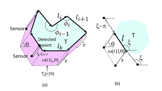
Figure 1: Illustration of locations of sensor of which sensing result is less than or equal to $r$

Let $\omega(r|\theta,l)\subset\mathbb{R}^{2}$ be the region where a sensor lies with $s\leq r$ and direction $\theta$, and the sensor’s detected point is on the line segment of length $l$ (Fig. 1-(b)). Note that $\omega(r|\theta,l)$ is a parallelogram of edge lengths $r$ and $l$. As shown in Fig. 1-(a), $\omega(r|\theta,l)$ is a component of $T_{s}(r|\theta)$ where, for a given $\theta$,

$$T_{s}(r|\theta)\stackrel{{\scriptstyle\mathrm{def}}}{{=}}\{(x,y)|0<\min_{(x+s\cos\theta,y+s\sin\theta)\in T}s\leq r\}.$$

When the direction of a line segment from the $x$-axis is $\xi$ ($0\leq\xi<2\pi$), the detected point is on this line segment if and only if $\xi-\pi\leq\theta\leq\xi$ for $r>0$ (Fig. 1-(b)). Then, for $0<r\leq r_{max}$ and fixed $\theta$,

$$|\omega(r|\theta,l)|_{2}=\cases{lr|\sin(\xi-\theta)|,&if $\xi-\pi\leq\theta\leq\xi$,\cr 0,&otherwise.}$$ (4)

Therefore,

$$|\omega(r|\theta,l)|_{3}=\int_{\xi-\pi}^{\xi}lr|\sin(\xi-\theta)|d\theta=2lr.$$ (5)

IV-A Analysis for convex $T$

For convex $T$, we derive $\Pr(s\leq r)$. Because of the convexity of $T$, $|T_{s}(r)|_{3}=\sum_{i}|\omega(r|\theta,l_{i})|_{3}$ (Fig. 1-(a)). Thus, according to Eq. (5),

$$|T_{s}(r)|_{3}=2\sum_{i}l_{i}r=2r|T|_{1}.$$ (6)

That is, $|\tilde{T}_{s}(r)|_{3}=2r|T|_{1}+2\pi|T|_{2}$. This is fundamentally equivalent to Eq. (6.48) in [santalo].

Therefore, we obtained the following result.

Theorem 1

For a convex target object $T$,

$$\Pr(s\leq r)=\frac{r|T|_{1}+\pi|T|_{2}}{\pi|\Omega|_{2}}.$$ (7)

IV-B Analysis for non-convex $T$

For non-convex $T$, we will derive $|T_{s}(r)|_{3}$. Assume that $\phi_{i}>\pi$, and focus on the $i$-th line segment in $\partial T$. See Fig. 2 where the $x$-axis is set along this line segment to make the analysis comprehensive (this is possible because we consider this line-segment only.) For $\phi_{i}>\pi$, as $\theta$ decreases, $\omega(r|\theta,l_{i})$ can overlap at the concave vertex $\phi_{i}$ by the $(i+1)$-th line segment. (The non-overlap part of $\omega(r|\theta,l_{i})$ is in pink in Fig. 2. For a large $\theta$, the whole $\omega(r|\theta,l_{i})$ is in pink. For a small $\theta$, only a small part is in pink.) Thus, $|T_{s}(r)|_{3}$ may not be equal to $\sum_{i}|\omega(r|\theta,l_{i})|_{3}$.

In this paper, events in which $\omega(r|\theta,l_{i})$ is limited by the $j$-th line segments within a sensing range are not taken into account, where $j\neq i-1,i+1$.

When $\theta<\phi_{i}-\pi$, $\omega(r|\theta,l_{i})$ overlaps with $T$ (Fig. 2). Let $v_{i}(r|\theta,l_{j})$ be the overlap between $\omega(r|\theta,l_{j})$ and $T$ around $\phi_{i}$ where $j=i,i+1$. In general, we need to take into account the effect of the overlaps to evaluate due to $|T_{s}(r)|_{3}$. Due to Eq. (5),

$$|T_{s}(r)|_{3}$$ (8)

$$= \sum_{i}(|\omega(r|\theta,l_{i})|_{3}-|v_{i}(r|\theta,l_{i})|_{3}-|v_{i}(r|\theta,l_{i+1})|_{3})$$ (9)

$$= 2r|T|_{1}-\sum_{i}\sum_{l=l_{i},l_{i+1}}|v_{i}(r|\theta,l)|_{3}.$$ (10)

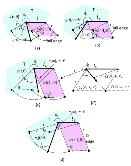
Figure 2: Illustration of cases for $\phi_{i}>\pi$

Consider the four exclusive cases to evaluate $|v_{i}(r|\theta,l_{i})|_{3}$ shown in Fig. 2 for $0<r\leq r_{max}$. Among the edges of $\omega(r|\theta,l_{i})$, consider the edge that is not parallel to the $i$-th line segment and the end point of which is at the connecting point between the $i$-th and $(i-1)$-th line segments. We call this edge the tail edge of $\omega(r|\theta,l_{i})$ because it is at the tail of the $i$-th line segment (Fig. 2). The former (latter) two cases correspond to the those in which the tail edge cannot (can) intersect the $(i+1)$-th line segment of $T$. If the tail edge does not intersect the line segment, the overlap $v_{i}(r|\theta,l_{i})$ is a triangle. However, if it intersects the line segment, the overlap becomes a quadrangle. Because the condition under which the tail edge can intersect the $(i+1)$-th line segment of $T$ depends on whether $\phi_{i}$ is larger than $3\pi/2$, we obtain four exclusive cases: whether $\phi>3\pi/2$ or not and whether the tail edge can intersect the $(i+1)$-th line segment or not. Calculation of $|v_{i}(r|\theta,l_{i})|_{3}$ is fundamentally the calculation of the size of the triangle or quadrangle. Therefore, the calculation does not require advanced mathematical knowledge, but it is messy and lengthy. The details are shown in Appendix LABEL:overlap_calculation.

Appendix LABEL:overlap_calculation and Eq. (10) provide us $|T_{s}(r)|_{3}$.

$$|T_{s}(r)|_{3}=2|T|_{1}r$$ (11)

$$-\sum_{k=12,3,4}\sum_{i}\sum_{l=l_{i},l_{i+1}}{\bf 1}(C_{k}(\phi_{i},l,r))g_{k}(\phi_{i},l,r).$$ (12)

That is, $|v_{i}(r|\theta,l)|_{3}=g_{k}(\phi_{i},l,r)$ if $C_{k}(\phi_{i},l,r)$ is true where $k=12,3,4$. Here,

$$C_{1}(\phi_{i},l_{i},r) \stackrel{{\scriptstyle\mathrm{def}}}{{=}} \{3\pi/2<\phi_{i}<2\pi,r<l_{i}|\sin\phi_{i}|\},$$

$$C_{2}(\phi_{i},l_{i},r) \stackrel{{\scriptstyle\mathrm{def}}}{{=}} \{\pi<\phi_{i}\leq 3\pi/2,r<l_{i}\},$$

$$C_{3}(\phi_{i},l_{i},r) \stackrel{{\scriptstyle\mathrm{def}}}{{=}} \{3\pi/2<\phi_{i}<2\pi,l_{i}|\sin\phi_{i}|\leq r\},$$

$$C_{4}(\phi_{i},l_{i},r) \stackrel{{\scriptstyle\mathrm{def}}}{{=}} \{\pi<\phi_{i}\leq 3\pi/2,l_{i}\leq r\},$$

$$C_{12}(\phi_{i},l_{i},r) \stackrel{{\scriptstyle\mathrm{def}}}{{=}} C_{1}(\phi_{i},l_{i},r)\cup C_{2}(\phi_{i},l_{i},r),$$

$$g_{1}(\phi_{i}) \stackrel{{\scriptstyle\mathrm{def}}}{{=}} -2+2(\phi_{i}-\pi)/\tan\phi_{i},$$

$$g_{12}(\phi_{i},r) \stackrel{{\scriptstyle\mathrm{def}}}{{=}} -r^{2}g_{1}(\phi_{i})/8,$$

and $g_{k}(\phi_{i},l,r)$ ($k=3,4$) are defined at the top of the next page. There, $\arcsin$ takes a value between $-\pi/2$ and $\pi/2$.

$$\gamma(\phi_{i},l,r) \stackrel{{\scriptstyle\mathrm{def}}}{{=}} l\sin(2\pi-\phi_{i})/r,\quad\zeta_{1}(\phi_{i},l,r)\stackrel{{\scriptstyle\mathrm{def}}}{{=}}\phi_{i}-\pi-\arcsin\gamma(\phi_{i},l_{,}r),\quad\zeta_{2}(\phi_{i},l,r)\stackrel{{\scriptstyle\mathrm{def}}}{{=}}\phi_{i}-\pi-(\pi-\arcsin\gamma(\phi_{i},l,r)),$$

$$g_{3,1}(\phi_{i},l,r) \stackrel{{\scriptstyle\mathrm{def}}}{{=}} -2\gamma(\phi_{i},l,r)^{2}+\frac{1}{\tan\phi_{i}}(2\arcsin\gamma(\phi_{i},l,r)-2\gamma(\phi_{i},l,r)\sqrt{1-\gamma(\phi_{i},l,r)^{2}}),$$

$$g_{3,2}(\phi_{i},l,r) \stackrel{{\scriptstyle\mathrm{def}}}{{=}} \frac{1}{\tan\phi_{i}}(-2(-\arcsin\gamma(\phi_{i},l,r)-\phi_{i}+2\pi)-2\gamma(\phi_{i},l,r)\sqrt{1-\gamma(\phi_{i},l,r)^{2}}-\sin(2\phi_{i}))$$

$$-1+2\gamma(\phi_{i},l,r)^{2}+\cos(2\phi_{i}),$$

$$g_{3,3}(\phi_{i},l,r) \stackrel{{\scriptstyle\mathrm{def}}}{{=}} \frac{l^{2}\sin\phi_{i}}{2}(\zeta_{1}(\phi_{i},l,r)\cos\phi_{i}-\sin\phi_{i}(\log|\sin(\phi_{i})|-\log(\gamma(\phi_{i},l,r)))),$$

$$g_{3,4}(\phi_{i},l,r) \stackrel{{\scriptstyle\mathrm{def}}}{{=}} \frac{l^{2}\sin\phi_{i}}{2}(\pi-2\arcsin\gamma(\phi_{i},l,r))\cos\phi_{i},$$

$$g_{3}(\phi_{i},l,r) \stackrel{{\scriptstyle\mathrm{def}}}{{=}} lr(\cos([\zeta_{2}(\phi_{i},l,r)]^{+})-\cos(\zeta_{1}(\phi_{i},l,r)))-\frac{r^{2}}{8}g_{3,1}(\phi_{i},l,r)$$

$$+(-\frac{r^{2}}{8}g_{3,2}(\phi_{i},l,r)+g_{3,4}(\phi_{i},l,r)){\bf 1}(\zeta_{2}(\phi_{i},l,r)>0)+g_{3,3}(\phi_{i},l,r){\bf 1}(\zeta_{2}(\phi_{i},l,r)\leq 0),$$

$$g_{4}(\phi_{i},l,r) \stackrel{{\scriptstyle\mathrm{def}}}{{=}} lr(1-\cos\zeta_{1}(\phi_{i},l,r))-\frac{r^{2}}{8}g_{3,1}(\phi_{i},l,r)+g_{3,3}(\phi_{i},l,r),$$

The meaning of the second term of the right-hand side of Eq. (12) is as follows. For a convex $\phi_{i}$ and $i$-th line segment (or $(i+1)$-th line segment), one of three conditions $C_{12}(\phi_{i},l,r)$, $C_{3}(\phi_{i},l,r)$, or $C_{4}(\phi_{i},l,r)$ becomes true for a given $r$. When $C_{k}(\phi_{i},l,r)$ becomes true, $g_{k}$ provides the effect of the overlap $|v_{i}(r|\theta,l_{i})|_{3}$ (or $|v_{i}(r|\theta,l_{i+1})|_{3}$) at $\phi_{i}$ and the $i$-th line segment (or $(i+1)$-th line segment).

Due to Eq. (3), we obtained the following result.

Theorem 2

For a polygon $T$ with angles $\{\phi_{i}\}_{i}$ and line segment lengths $\{l_{i}\}_{i}$,

$$\Pr(s\leq r)$$ (13)

$$= \frac{1}{2\pi|\Omega|_{2}}\{2|T|_{1}r+2\pi|T|_{2}$$ (15)

$$-\sum_{k=12,3,4}\sum_{i}\sum_{l=l_{i},l_{i+1}}{\bf 1}(C_{k}(\phi_{i},l,r))g_{k}(\phi_{i},l,r)\}.$$

V Observability

In this paper, we use the following definition of observability and discuss what parameters of a target object we can estimate. If some parameters are not observable, we cannot estimate them even with a huge number of sensors and with a sophisticated estimation method.

Definition of Observability Let $\Pr(s\leq r|\rho,\rho^{\prime})$ be $\Pr(s\leq r)$ when parameter vectors $\rho$ and $\rho^{\prime}$ are given. A parameter vector $\rho$ is observable if and only if there exists a finite set of values $\{\Pr(s\leq s_{i}|\rho,\rho^{\prime})\}_{i}$ that can uniquely determine $\rho$.

V-A Observability for convex $T$

Theorem 3

When we know that $T$ is convex, $|T|_{1}$ and $|T|_{2}$ are observable and parameters other than $|T|_{1}$ and $|T|_{2}$ are not observable.

Proof:

Because sensors are independently deployed, the sensing result of each sensor is a random sample of which probability distribution is $\Pr(s\leq r)$. Due to Eq. (7), it is clear that $|T|_{1}$ and $|T|_{2}$ are observable. However, parameters other than $|T|_{1}$ and $|T|_{2}$ are not observable because Eq. (7) is determined only by $|T|_{1}$ and $|T|_{2}$. $\square$

Because $|T|_{1}$ and $|T|_{2}$ are observable but other parameters are not observable by using randomly deployed binary sensors [infocom], this theorem implies that the parameter space that we can estimate cannot be increased even by distance sensors for convex $T$.

V-B Observability for general $T$

For a general polygon $T$, we will derive observable parameters and the conditions that $\{l_{i},l_{i+1},\phi_{i}>\pi\}_{i}$ are observable.

Theorem 4

$|T|_{1}$, $|T|_{2}$, and convexity are observable.