KIAS-P17055
Neutrino mass in flavor dependent gauged lepton model
Abstract
We study a neutrino model introducing an additional nontrivial gauged lepton symmetry where the neutrino masses are induced at two-loop level while the first and second charged-leptons of the standard model are done at one-loop level. As a result of model structure, we can predict one massless active neutrino, and there is a dark matter candidate. Then we discuss neutrino mass matrix, muon anomalous magnetic moment, lepton flavor violations, oblique parameters, and relic density of dark matter taking into account the experimental constraints.
I Introduction
A flavor dependent gauge model often plays an important role in explaining flavor specific measurements such as deviation from the standard model (SM) in semileptonic decay process which is reported by LHCb Aaij:2014ora ; Aaij:2017vbb , lepton flavor violations (LFVs) such as process TheMEG:2016wtm , and muon anomalous magnetic moment() at Brookhaven National Laboratory Bennett:2006fi . Along thought of these ideas, the ref. Crivellin:2016ejn has established a flavor dependent model with a larger gauge group, and a smaller group such as flavor dependent model can be found as a result of partially breaking the symmetry.
In particular, it is interesting to consider active neutrino mass matrix with a lepton specific flavor dependent gauge symmetry in the ref. Crivellin:2016ejn . The active neutrino masses are not allowed at the tree level and it should be related to the gauge symmetry breaking. Then a radiative seesaw scenario is an attractive candidate to generate the mass, which can be achieved introducing some exotic particles. Furthermore we expect predictability in the active neutrino mass due to restriction from the gauge symmetry.
In this paper, we construct a neutrino model based on the lepton flavor symmetry , where the neutrino mass can be induced at two-loop level 2-lp-zB ; Babu:2002uu ; AristizabalSierra:2006gb ; Nebot:2007bc ; Schmidt:2014zoa ; Herrero-Garcia:2014hfa ; Long:2014fja ; VanVien:2014apa ; Aoki:2010ib ; Lindner:2011it ; Baek:2012ub ; Aoki:2013gzs ; Kajiyama:2013zla ; Kajiyama:2013rla ; Baek:2013fsa ; Okada:2014vla ; Okada:2014qsa ; Okada:2015nga ; Geng:2015sza ; Kashiwase:2015pra ; Aoki:2014cja ; Baek:2014awa ; Okada:2015nca ; Sierra:2014rxa ; Nomura:2016rjf ; Nomura:2016run ; Bonilla:2016diq ; Kohda:2012sr ; Dasgupta:2013cwa ; Nomura:2016ask ; Nomura:2016pgg ; Liu:2016mpf ; Nomura:2016dnf ; Simoes:2017kqb ; Baek:2017qos ; Ho:2017fte ; Nomura:2017xko ; Guo:2017gxp ; delAguila:2011gr . We first discuss the case of general charge assignment and the conditions to cancel gauge anomalies. Then phenomenological analysis is carried out by fixing the charge assignment for our particle contents. As a result we predict one massless active neutrino, and discuss a dark matter candidate calculating relic density. In addition, we discuss lepton flavor violations (LFVs) and muon in the model.
This paper is organized as follows. In Sec. II, we show the mechanism of anomaly cancellations, review our model setup, formulate the Higgs sector, fermion sector including active neutrinos, muon anomalous magnetic moment, lepton flavor violations, and phenomenologies of a dark matter candidate where we show the allowed region of DM mass to satisfy the relic density without conflict of direct detection bound. In Sec. III, we have globally numerical analysis, and investigate the allowed region to satisfy all the data that we will discuss. Finally we devote Sec. IV to conclusion.
II Model setup and phenomenologies
Here we construct our model with symmetry and carry out phenomenological analysis. In fermion sector, we introduce three exotic singly-charged fermions with different charges; and respectively have and , while , which is a vector-like fermion, has . Notice here that the charge of is arbitrary in general, but are determined by several anomaly cancellations as discussed below. In boson sector, we introduce three isospin singlet bosons with nonzero VEVs, and and respectively have and . In addition, we introduce a singly charged boson , a doubly charged boson , and an isospin singlet(doublet) inert boson , and each of them has charge of , , and . is identified as the SM-like Higgs. Furthermore, we impose odd for new fields except and in order to forbid the mixing between the SM fermions and exotic one and assure the stability of DM candidate; neutral component of . Thus neutrino masses are induced at two-loop level as shown below. These particle contents and its charge assignments are summarized in Table 1.
Anomaly cancellation: We explore conditions of anomaly cancellations under the gauge symmetry in table 1, where is automatically zero under these symmetries. Thus one should consider three types of triangle anomalies including all the families as follows:
| (II.1) | |||
| (II.2) | |||
| (II.3) | |||
| (II.4) |
Therefore one finds the following two conditions:
| (II.5) |
One finds several simple solutions such as that respectively correspond to and symmetry for lepton doublets.
Fixing charge assignments: Here we fix to be and for simplicity. In this case, one can simply define with charge of . Under these symmetries in table 1, the renormalizable Lagrangian in the lepton sector and Higgs potential are respectively given by
| (II.6) | |||
| (II.7) | |||
| (II.8) |
| (II.9) |
where runs over to , and run over to , with being the second Pauli matrix. The first term gives the masses for the SM charged-leptons, and as well as and contribute to the structure of neutrino masses. forbids the massless goldstone boson (GB) arising from . On the other hand does not contribute to the neutrino masses and itself cannot reproduce the experimental results for neutrinos. Thus we just neglect these terms in our analysis.
Next we formulate the scalar sector, in which we parameterize as follows:
| (II.14) |
where , and two massless eigenstates among , and are absorbed by the SM and gauge bosons , , and . Inserting tadpole conditions, the CP even mass matrix in basis of can be formulated by , where is the SM Higgs and is three by three orthogonal mixing matrix. On the other hand the inert boson mass matrix in basis of is formulated by , where is two by two orthogonal matrix. Then one can parametrize the relation between flavor and mass eigenstate as Okada:2014qsa
| (II.21) |
where is proportional to , and we expect to be in our analysis below. On the other hand the singly charged boson mass matrix in basis of is formulated by , where is two by two orthogonal matrix. 111In general it should be unitary. But it can be orthogonal when all the coupling of Higgs potential are real. Then one can parametrize the relation between flavor and mass eigenstate as Okada:2014qsa
| (II.28) |
where is proportional to .
boson: A massive boson appears after spontaneous symmetry breaking of . The mass of is given by where is gauge coupling of . Since the couples to electrons the mass and gauge coupling are constrained by the LEP data. Here we simply assume the mass is around TeV scale and the value of satisfies the constraints. Note that does not contribute to neutrino mass generation and our DM candidate has no direct interaction with the since does not have charge. Thus we will not discuss physics in our analysis.
Exotic charged-fermion masses: After the symmetry breaking, the exotic charged fermion mass matrix in Eq.(II.7) can be given in the basis as follows:
| (II.32) |
where we have assumed to be a real symmetric matrix for simplicity and define , , , and . Then is diagonalized by an orthogonal mixing matrix () as
| (II.33) |
where is the mass eigenstate.
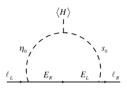
SM charged-fermion masses: Since the first and second charged-leptons are not induced at the tree level, but done at the one-loop level in fig. 1. In order to formulate these masses, let us write down the relevant Lagrangian to the SM charged-leptons in the mass eigenbasis as
| (II.34) |
where . Then the mass matrix for the charged-leptons can be induced as follows Nomura:2016emz ; Nomura:2016pgg ; Nomura:2017ezy :
| (II.35) | |||
| (II.36) |
is generally diagonalized by bi-unitary matrices as , where is mass eigenstate of charged-leptons. Then the resulting mass eigenvalues for the SM charged-leptons are generally given by
| (II.37) |
Thus the observed lepton mixing arises from the neutrino part only.
Active neutrinos: First of all, let us write down the relevant Lagrangian to the neutrinos in the mass eigenbasis as
| (II.38) |
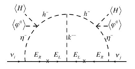
where is the rank two matrix. Then the neutrino mass matrix is induced at the two-loop level in fig. 2, which is given by Okada:2014qsa
| (II.39) | |||
| (II.40) |
where , , and . Whereas we also formulate the experimental neutrino mass matrix as that can be determined by neutrino oscillation data, when numerical (Dirac and Majorana) phases are provided. Notice here that one of the three active neutrino mass eigenstates is massless, since the matrix rank is two; in case of normal(inverted) hierarchy. The structure of the mass matrix indicate that the neutrino mixing angles mainly arise from the mixing matrix . Then one finds the following ranges at 3 confidential level Forero:2014bxa given by 222Recently is experimentally favored. But our result does not change significantly, even if we fix to be ., assuming the normal one:
| (II.44) |
and Majorana phases taken to be . In the numerical analysis, we impose the constraint .
Muon anomalous magnetic moment (): has been observed and its discrepancy is estimated by Hagiwara:2011af
| (II.45) |
The relevant Yukawa Lagrangian contributing to as well as LFVs in the mass eigenbasis is given by
| (II.46) |
where and . Then our is induced by interaction with coupling as explained above, and its form is computed as
| (II.47) | ||||
| (II.48) |
Considering the neutrino oscillations and lepton flavor violations for term as will be discussed below, we find the maximal order of to be . On the other hand the term with provides the dominant contribution to , since it is not constrained by any phenomenologies once we take .
In addition, gauge boson can contribute to and its form is approximately given by
| (II.49) |
where is the new gauge vector boson. Since the right-handed electron couples to the boson, we have the constraint Nomura:2017tih ; the maximal value of is . Combining and , we find the final result of muon ; , where we will adapt the maximal value in our numerical analysis below.
Lepton flavor violations (LFVs): LFV processes of are given by the same term as the , and their forms are given by
| (II.50) |
where is the fine-structure constant, GeV-2 is the Fermi constant, and , , . Experimental upper bounds are given by TheMEG:2016wtm ; Adam:2013mnn :
| (II.51) |
where we define , , and .
Oblique parameter: Since we have an isospin doublet boson , we have to consider the oblique parameter known as and Barbieri:2006dq . In our case, one finds the following relations:
| (II.52) |
where let us remind the conditions ; and . Then the current bounds are given by Cheung:2017efc
| (II.53) |
Dark matter: In our model, we have two types of DM candidates; and . But let us here focus on the neutral component of can be DM candidate resymbolized by , because is more testable than due to constraining the mass than from experiments such as neutrino oscillations, LFVs, and oblique parameters. Although the general analysis has been done by Ref. Hambye:2009pw , we impose a constraint of the DM mass, which is smaller than the mass of boson, but greater than the half of Z boson mass to forbid the invisible decay of Z boson; therefore
| (II.54) |
This region is in favor of getting sizable muon , and well testable in the direct detection constraint such as LUX experiment Akerib:2016vxi because it provides the most severe bound at around 50 GeV. Under the condition, we have two relevant annihilation cross sections to explain the relic density of DM. One mode arises from Yukawa coupling that gives the d-wave dominance, and another one does from s-channel via SM Higgs with final state of bottom pairs, where we assume mixing among the CP-even neutral bosons are negligible. The wave dominant cross section given by Eq. (II.46) is found to be Das:2017ski
| (II.55) |
In our estimation, however, this cross section reaches [GeV]-2 at most, which is smaller than the cross section required to give right relic density by one order of magnitude. Thus we have to rely on Higgs portal interaction mode, and its dimensionless cross section is found to be
| (II.56) | |||
| (II.57) |
where is the trilinear couplings of , arising from . Notice here that is restricted by the direct detection with spin independent scattering via Higgs portal, 333The constraint of invisible decay of the SM Higgs always gives milder than the one of direct detection in our parameter region. Thus we will not discuss here. and its bound is conservatively found to be Das:2017ski
| (II.58) |
Here we apply the following formula to get the relic density of DM given by Edsjo:1997bg ;
| (II.59) |
where is the degrees of freedom for relativistic particles at temperature , GeV, and is given by Nishiwaki:2015iqa
| (II.60) |
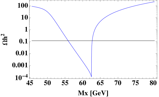
where GeV is the Planck mass, is the total number of effective relativistic degrees of freedom at the time of freeze-out, and is defined by at the freeze out temperature (). Then one has to satisfy the the current relic density of DM; Ade:2013zuv . In fig. 3, we show the line of in terms of , where we have used the maximum value in Eq.(II.58); . Thus one finds that the resulting allowed region is
| (II.61) |
where the upper bound of the DM mass; , arises from the pole mass of the half SM Higgs.

III Numerical analysis
In this section, we show a global analysis. Before the numerical analysis, we work on the diagonal basis of by the phase redefinition of ; Diag.(). Then we directly solve the couplings and by using the relations and , respectively, where we impose the perturbative bounds on these output parameters; . 444In principle, all the Yukawa couplings could be solved by using all the components of these relations. However it is technically difficult in our model. Now we randomly select the following range of reduced input parameters as
| (III.1) |
where the lower mass range for arises from the bound from LEP data Abbiendi:2008aa , while the upper bound from the oblique parameters, and we impose all the constraints as discussed above.
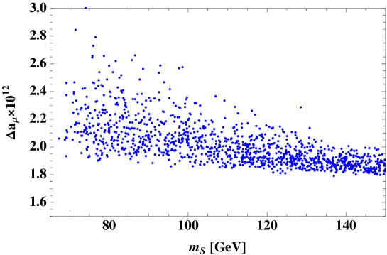
In Fig. 4, we show the scattering allowed plots in terms of muon and . It suggests that the typical value of muon is of the order that is smaller than the experimental value by three order magnitude.
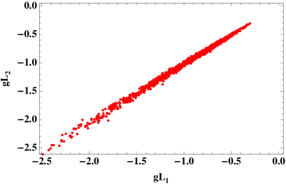
In Fig. 5, we demonstrate the couplings of in the left-figure, and in the right-figure. The left one implies requires rather large coupling, whereas is of the order 0.001, and each of them has a weak correlation. While the right one suggests both of couplings run with degeneracy to some extent.
IV Conclusion
We have constructed radiative neutrino mass model based on a gauged lepton flavor symmetry . The condition to cancel gauge anomalies is discussed by introducing some exotic leptons with general charge. Then we discuss phenomenology of the model by fixing the charge assignment.
The neutrino mass matrix can be induced at two-loop level where the exotic leptons and charged scalar bosons propagate inside the loop diagram. On the other hand the first and second charged-leptons of SM are induced at one-loop level. Due to the feature of flavor dependent symmetry, we have predicted one massless active neutrino and a bosonic dark matter candidate from inert doublet. Calculating the relic density, we have found that observed value can be obtained via Higgs portal interaction with mass range of dark matter at GeV GeV. In addition, we have also discussed lepton flavor violation and muon in the model.
Then we have done the global numerical analysis to satisfy all the constraints such as charged-lepton masses, neutrino mass differences its mixing, LFVs, and oblique parameters, within the range of DM mass. Then we have found the typical value of muon is of the order that is smaller than the experimental value by three order magnitude. Also we have shown the typical Yukawa couplings of and , and found typical ranges and their correlations.
Acknowledgments
H. O. is sincerely grateful for the KIAS member and all around.
References
- (1) R. Aaij et al. [LHCb Collaboration], Phys. Rev. Lett. 113, 151601 (2014) [arXiv:1406.6482 [hep-ex]].
- (2) R. Aaij et al. [LHCb Collaboration], arXiv:1705.05802 [hep-ex].
- (3) A. M. Baldini et al. [MEG Collaboration], Eur. Phys. J. C 76, no. 8, 434 (2016) [arXiv:1605.05081 [hep-ex]].
- (4) G. W. Bennett et al. [Muon g-2 Collaboration], Phys. Rev. D 73, 072003 (2006) [hep-ex/0602035].
- (5) A. Crivellin, J. Fuentes-Martin, A. Greljo and G. Isidori, Phys. Lett. B 766, 77 (2017) [arXiv:1611.02703 [hep-ph]].
- (6) A. Zee, Nucl. Phys. B 264, 99 (1986); K. S. Babu, Phys. Lett. B 203, 132 (1988).
- (7) K. S. Babu and C. Macesanu, Phys. Rev. D 67, 073010 (2003) [hep-ph/0212058].
- (8) D. Aristizabal Sierra and M. Hirsch, JHEP 0612, 052 (2006) [hep-ph/0609307].
- (9) M. Nebot, J. F. Oliver, D. Palao and A. Santamaria, Phys. Rev. D 77, 093013 (2008) [arXiv:0711.0483 [hep-ph]].
- (10) D. Schmidt, T. Schwetz and H. Zhang, Nucl. Phys. B 885, 524 (2014) [arXiv:1402.2251 [hep-ph]].
- (11) J. Herrero-Garcia, M. Nebot, N. Rius and A. Santamaria, Nucl. Phys. B 885, 542 (2014) [arXiv:1402.4491 [hep-ph]].
- (12) H. N. Long and V. V. Vien, Int. J. Mod. Phys. A 29, no. 13, 1450072 (2014) [arXiv:1405.1622 [hep-ph]].
- (13) V. Van Vien, H. N. Long and P. N. Thu, arXiv:1407.8286 [hep-ph].
- (14) M. Aoki, S. Kanemura, T. Shindou and K. Yagyu, JHEP 1007, 084 (2010) [Erratum-ibid. 1011, 049 (2010)] [arXiv:1005.5159 [hep-ph]].
- (15) M. Lindner, D. Schmidt and T. Schwetz, Phys. Lett. B 705, 324 (2011) [arXiv:1105.4626 [hep-ph]].
- (16) S. Baek, P. Ko, H. Okada and E. Senaha, JHEP 1409, 153 (2014) [arXiv:1209.1685 [hep-ph]].
- (17) M. Aoki, J. Kubo and H. Takano, Phys. Rev. D 87, no. 11, 116001 (2013) [arXiv:1302.3936 [hep-ph]].
- (18) Y. Kajiyama, H. Okada and K. Yagyu, Nucl. Phys. B 874, 198 (2013) [arXiv:1303.3463 [hep-ph]].
- (19) Y. Kajiyama, H. Okada and T. Toma, Phys. Rev. D 88, 015029 (2013) [arXiv:1303.7356].
- (20) S. Baek, H. Okada and T. Toma, JCAP 1406, 027 (2014) [arXiv:1312.3761 [hep-ph]].
- (21) H. Okada, arXiv:1404.0280 [hep-ph].
- (22) H. Okada, T. Toma and K. Yagyu, Phys. Rev. D 90, no. 9, 095005 (2014) [arXiv:1408.0961 [hep-ph]].
- (23) H. Okada, arXiv:1503.04557 [hep-ph].
- (24) C. Q. Geng and L. H. Tsai, arXiv:1503.06987 [hep-ph].
- (25) S. Kashiwase, H. Okada, Y. Orikasa and T. Toma, Int. J. Mod. Phys. A 31, no. 20n21, 1650121 (2016) [arXiv:1505.04665 [hep-ph]].
- (26) M. Aoki and T. Toma, JCAP 1409, 016 (2014) [arXiv:1405.5870 [hep-ph]].
- (27) S. Baek, H. Okada and T. Toma, Phys. Lett. B 732, 85 (2014) [arXiv:1401.6921 [hep-ph]].
- (28) H. Okada and Y. Orikasa, Phys. Rev. D 93, no. 1, 013008 (2016) [arXiv:1509.04068 [hep-ph]].
- (29) D. Aristizabal Sierra, A. Degee, L. Dorame and M. Hirsch, JHEP 1503, 040 (2015) [arXiv:1411.7038 [hep-ph]].
- (30) T. Nomura and H. Okada, Phys. Lett. B 756, 295 (2016) [arXiv:1601.07339 [hep-ph]].
- (31) T. Nomura, H. Okada and Y. Orikasa, arXiv:1602.08302 [hep-ph].
- (32) C. Bonilla, E. Ma, E. Peinado and J. W. F. Valle, arXiv:1607.03931 [hep-ph].
- (33) M. Kohda, H. Sugiyama and K. Tsumura, Phys. Lett. B 718, 1436 (2013) [arXiv:1210.5622 [hep-ph]].
- (34) B. Dasgupta, E. Ma and K. Tsumura, Phys. Rev. D 89, 041702 (2014) [arXiv:1308.4138 [hep-ph]].
- (35) T. Nomura and H. Okada, Phys. Rev. D 94, 075021 (2016) [arXiv:1607.04952 [hep-ph]].
- (36) T. Nomura and H. Okada, arXiv:1609.01504 [hep-ph].
- (37) T. Nomura, H. Okada and Y. Orikasa, Phys. Rev. D 94, no. 11, 115018 (2016) [arXiv:1610.04729 [hep-ph]].
- (38) Z. Liu and P. H. Gu, arXiv:1611.02094 [hep-ph].
- (39) C. Simoes and D. Wegman, arXiv:1702.04759 [hep-ph].
- (40) S. Baek, H. Okada and Y. Orikasa, arXiv:1703.00685 [hep-ph].
- (41) S. Y. Ho, T. Toma and K. Tsumura, arXiv:1705.00592 [hep-ph].
- (42) T. Nomura and H. Okada, arXiv:1706.01321 [hep-ph].
- (43) S. Y. Guo, Z. L. Han, B. Li, Y. Liao and X. D. Ma, arXiv:1707.00522 [hep-ph].
- (44) F. del Aguila, A. Aparici, S. Bhattacharya, A. Santamaria and J. Wudka, JHEP 1205, 133 (2012) doi:10.1007/JHEP05(2012)133 [arXiv:1111.6960 [hep-ph]].
- (45) T. Nomura and H. Okada, Phys. Lett. B 761, 190 (2016) doi:10.1016/j.physletb.2016.08.023 [arXiv:1606.09055 [hep-ph]].
- (46) T. Nomura and H. Okada, Phys. Rev. D 96, no. 1, 015016 (2017) [arXiv:1704.03382 [hep-ph]].
- (47) J. A. Casas and A. Ibarra, Nucl. Phys. B 618, 171 (2001) doi:10.1016/S0550-3213(01)00475-8 [hep-ph/0103065].
- (48) D. V. Forero, M. Tortola and J. W. F. Valle, Phys. Rev. D 90, no. 9, 093006 (2014) [arXiv:1405.7540 [hep-ph]].
- (49) K. Hagiwara, R. Liao, A. D. Martin, D. Nomura and T. Teubner, J. Phys. G 38, 085003 (2011) [arXiv:1105.3149 [hep-ph]].
- (50) T. Nomura and H. Okada, arXiv:1707.00929 [hep-ph].
- (51) J. Adam et al. [MEG Collaboration], Phys. Rev. Lett. 110, 201801 (2013) [arXiv:1303.0754 [hep-ex]].
- (52) R. Barbieri, L. J. Hall and V. S. Rychkov, Phys. Rev. D 74, 015007 (2006) [hep-ph/0603188].
- (53) K. Cheung, T. Nomura and H. Okada, Phys. Lett. B 768, 359 (2017) [arXiv:1701.01080 [hep-ph]].
- (54) T. Hambye, F.-S. Ling, L. Lopez Honorez and J. Rocher, JHEP 0907, 090 (2009) Erratum: [JHEP 1005, 066 (2010)] [arXiv:0903.4010 [hep-ph]].
- (55) D. S. Akerib et al. [LUX Collaboration], Phys. Rev. Lett. 118, no. 2, 021303 (2017) [arXiv:1608.07648 [astro-ph.CO]].
- (56) A. Das, T. Nomura, H. Okada and S. Roy, arXiv:1704.02078 [hep-ph].
- (57) J. Edsjo and P. Gondolo, Phys. Rev. D 56, 1879 (1997) [hep-ph/9704361].
- (58) K. Nishiwaki, H. Okada and Y. Orikasa, Phys. Rev. D 92, no. 9, 093013 (2015) [arXiv:1507.02412 [hep-ph]].
- (59) P. A. R. Ade et al. [Planck Collaboration], Astron. Astrophys. 571, A16 (2014) [arXiv:1303.5076 [astro-ph.CO]].
- (60) G. Abbiendi et al. [OPAL Collaboration], Eur. Phys. J. C 72, 2076 (2012) [arXiv:0812.0267 [hep-ex]].