Pinning of a drop by a junction on an incline

Abstract

The shape of a drop pinned on an inclined substrate is a long-standing problem where the complexity of real surfaces, with heterogeneities and hysteresis, makes it complicated to understand the mechanisms behind the phenomena. Here we consider the simple case of a drop pinned on an incline at the junction between a hydrophilic half-plane (the top half) and a hydrophobic one (the bottom half). Relying on the equilibrium equations deriving from the balance of forces, we exhibit three scenarii depending on the way the contact line of the drop on the substrate either simply leans against the junction or overfills (partly or fully) into the hydrophobic side. We draw some conclusions on the geometry of the overlap and the stability of these tentative equilibrium states. In the corresponding retention force factor, we find that a major role is played by the wetted length of the junction line, in the spirit of Furmidge’s observations. The predictions of the theory are compared with extensive molecular dynamics simulations.

1 Introduction

As first described by Thomas Young [30] in his essay on cohesion of fluids in 1805, the competition between the cohesion of a fluid to itself and its adhesion to a solid gives rise to an angle of contact $\theta_{0}$ between the liquid and the solid that is specific to a given system at equilibrium. This is now well known as the Young equation:

$$\gamma\cos\theta_{0}=\gamma_{SV}-\gamma_{SL}$$ (1)

where $\theta_{0}$ is the equilibrium contact angle and $\gamma_{SV}$ and $\gamma_{SL}$ are the Solid-Vapor and Solid-Liquid surface tensions, respectively. It has been proven recently that this equation holds down to the nanometric scale [7, 27, 10]. In practice however, this equation holds for pure liquids on flat glasses or silica wafers. For real heterogeneous surfaces, chemically or physically, the situation is more complex. We have to introduce the advancing ($\theta^{A}$), the receding ($\theta^{R}$) static contact angles and the difference between both, which is called the hysteresis and arises from surface roughness and/or heterogeneity [29, 15, 17, 16, 23]. The contact angle of a sessile drop actually observed will lie between $\theta^{A}$ to $\theta^{R}$ and is function of the process of reaching the particular equilibrium state. See [11] for background and references.

The variety of possible processes and motions makes the prediction of the final static contact angle challenging. No generally applicable correlation between hysteresis and roughness features is known for a given surface. When the corresponding substrate is tilted by a small angle $\alpha$, the drop usually deforms its shape but remains pinned on the substrate. It is only when the tilt angle $\alpha$ becomes large enough, above the value $\alpha_{c}$, that the drop starts to slide. It has been proposed by Furmidge [14], Eq. $5,$ that

$$mg\sin\alpha_{c}=\frac{k}{2}w\gamma(\cos\theta^{R}-\cos\theta^{A})$$ (2)

where $m$ is the mass of the drop, $g$ the gravity constant, $\theta^{R}$ and $\theta^{A}$ the receding and the advancing contact angles, $w$ the width of the drop in the direction perpendicular to inclination. The dimensionless retention-force factor $k$ is close to $2$ according to [14], Table $2$, but its value has been reexamined since then ([6] Eq. $27$; [12] Eq. $1$, [13] Eq. $1$, [22] Eq. $3$, [28] Eq. $4$ and [9] Eqs. $1$ and $2$), concluding to $k$ varying in the range $\pi/2\leq k\leq 2$, depending on the physical situation. Several studies have been devoted to this equation through experiments [1], numerical or theoretical calculations [24]. Mostly, all these studies differ by their hypothesis concerning the shape of the contact line or different conditions for the experiments.

We are herewith studying the basic case where there is a chemical step in the substrate. Experimentally this is a difficult situation simply because the difference of wettability will be associated to a zone and not to a line. To explore in details the validity of equations like Eq. (2) avoiding unnecessary hypothesis, it is interesting to revisit this problem using large scale molecular dynamics.

The problem of a drop on an incline at the junction between a hydrophilic half-plane and a hydrophobic half-plane has been addressed previously, notably by simulation with Surface Evolver. See [2], [3] and references therein. An inclined chemical step has also been considered in [25]. The incline has also been replaced by a wettability gradient [19].

The paper is organized as follows. The theoretical aspects are given in Section 2. Then we present the corresponding molecular dynamics simulations in Section 3. Section 4 is devoted to a comparison between the two approaches. Finally, some concluding remarks are presented in Section 5.

2 Drop on incline at hydrophilic-hydrophobic junction: theory

2.1 Drop pinned on inhomogeneous incline

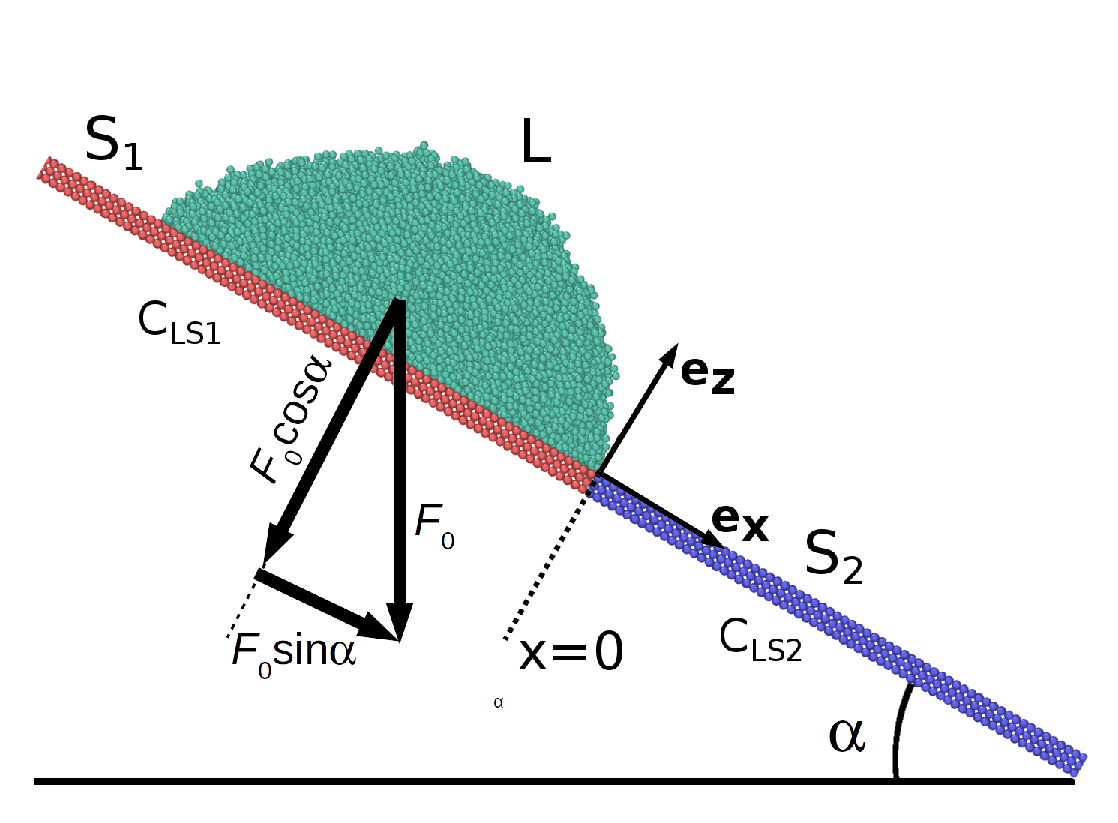
Figure 1: Scheme of the liquid drop on incline plane close to the boundary between two solids under an external force $F_{0}$.

We first study the case of a drop pinned on an arbitrary inhomogeneous incline. While considering the total capillary force, the gravity force and the total pressure force acting upon the drop sum up to zero at equilibrium, we obtain, while projecting on each axis relative to the incline, a system of three equations relating the gravity force components to contour integrals along the contact line and with a pressure contribution in the direction perpendicular to the incline. In more details we consider an incline of angle $\alpha$ with respect to the horizontal. The $x$-axis is along the slope downhill, the $y$-axis is horizontal, the $z$-axis is perpendicular to the incline. The corresponding orthonormal basis is $\mathbf{e_{x}},\mathbf{e_{y}},\mathbf{e_{z}}$ as in Fig. 1. The basis of the drop is denoted $\Omega$ and its boundary, the contact line $\partial\Omega$, is assumed piecewise differentiable, and $\mathbf{n}$ is the outer normal to the contact line in the substrate plane. The contact angle $\theta$ is assumed piecewise continuous on $\partial\Omega$. The total capillary force $\mathbf{F}$ upon the drop is

$$\mathbf{F}=\gamma\,\oint_{\partial\Omega}\,dl\,(\mathbf{n}\cos\theta-\mathbf{e_{z}}\sin\theta)$$ (3)

The gravity force upon the drop is

$$m\mathbf{g}=(mg\sin\alpha,\,0,\,-mg\cos\alpha)$$

The total pressure force upon the drop is

$$\mathbf{e_{z}}\int_{\Omega}dxdy\left(p(x,y,0)-p_{\mathrm{atm}}\right)$$ (4)

These formulae remain valid if the contact line has a slow motion so that the drop profile is always in the equilibrium shape conditioned by the instantaneous contact line. The pinning and depinning of the contact line depend upon $\gamma_{SV}-\gamma_{SL}$, where $\gamma_{SV}$ and $\gamma_{SL}$ are the local Solid-Vapor (air) and Solid-Liquid (water) surface tensions, which typically are not smooth functions, and which play a role in (3) only through the choice of the contact line $\partial\Omega$. Therefore, in these formulae, the contact angle $\theta$ can be any angle between the local advancing ($\theta^{A}$) and receding ($\theta^{R}$) angles.

At equilibrium the forces upon the drop sum up to zero, on each axis:

$$0 = mg\sin\alpha+\gamma\,\oint_{\partial\Omega}\,dl\,\mathbf{n}\cdot\mathbf{e_{x}}\,\cos\theta$$ (5)

$$0 = \oint_{\partial\Omega}\,dl\,\mathbf{n}\cdot\mathbf{e_{y}}\,\cos\theta$$ (6)

$$0 = -mg\cos\alpha-\gamma\,\oint_{\partial\Omega}dl\,\sin\theta+\int_{\Omega}dxdy\left(p(x)-p_{\mathrm{atm}}\right)$$ (7)

where $p(x)=p(x,y,0)=p(0,0,0)+\rho gx\sin\alpha$ from the law of hydrostatics. Equation (6) will be automatically satisfied for a drop symmetric with respect to the plane ${y=0}$, where $\mathbf{n}(x,\,-y)\cdot\mathbf{e_{y}}=-\mathbf{n}(x,\,y)\cdot\mathbf{e_{y}}$ and $\theta(x,-y)=\theta(x,y)$.

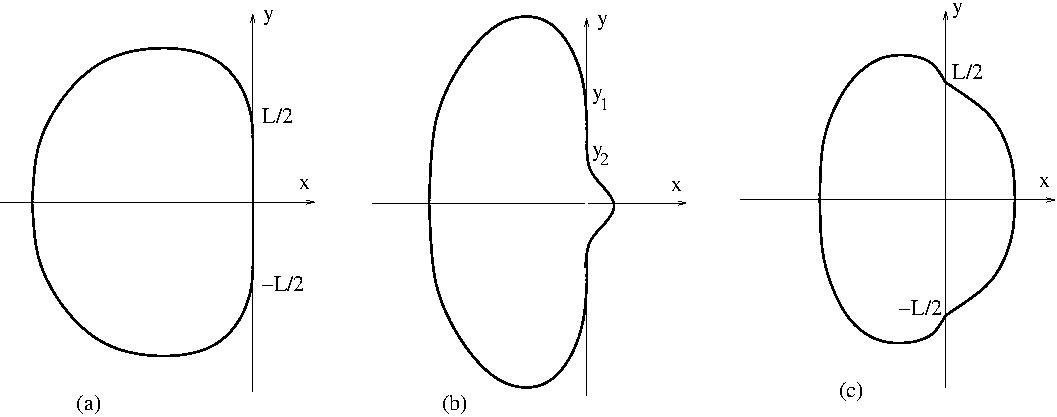
Figure 2: Contact line at hydrophilic-hydrophobic junction, gravity increased from (a) to (c): (a) stable equilibrium, Eq. (9); (b) tentative equilibrium, Eq. (12); (c) unstable equilibrium, Eq. (13).

2.2 Drop pinned at hydrophilic-hydrophobic junction

We next consider the same problem but specifically for a drop pinned on an incline at the junction between a hydrophilic half-plane (the top half) and a hydrophobic one (the bottom half). In this context, we discuss three scenarii: $\left(a\right)$ one for which the contact line partly follows the junction line on a segment of width $L$, $\left(b\right)$ one for which part of the contact line goes into the hydrophobic half-plane in a central protuberance while keeping two side overlaps with the junction line and $\left(c\right)$ one for which part of the contact line crosses straight into the hydrophobic half-plane. See Fig. 2.

The three cases may be viewed as the ones obtained while successively increasing the angle of the incline, or gravity or the volume of the drop, in short increasing the Bond number $Bo$. The first case can be a stable equilibrium, the second might be a stable equilibrium and the third is an unstable equilibrium.

In this hydrophilic/hydrophobic junction setup, we derive the new version of the equilibrium equations deriving from the balance of forces. For case $\left(a\right)$, equation (5) along the axis of the slope downhill equates the projection of the gravity force to a simple integral of the cosine of the contact angle over the overlap segment of unknown length $L$; observing that the contact angle is maximal in the middle of the overlap segment and bounded above by the Young angle in the hydrophobic side, a lower bound of $L$ is supplied. For case $\left(b\right)$, the same equation equates the projection of the gravity force to the sum of two contributions: one similar to the previous one but restricted to the overlap junction line/contact line and one relative to the protuberance involving the difference between the Young angle cosines in the hydrophilic/hydrophobic half-planes times the length of the junction line covered by the protuberance. Finally, for case $\left(c\right)$, there is only one contribution to the balance equation involving the difference between the Young angle cosines in the hydrophilic/hydrophobic half-planes times the full length of the junction line covered by the drop. Let us now formulate and justify this in details.

The upper half-plane $\{x<0\}$ is a relatively hydrophilic substrate, of Young angle $\theta_{1}$, while the lower half-plane $\{x>0\}$ is less hydrophilic, of Young angle $\theta_{2}>\theta_{1}$. The contact line is either $\partial\Omega=\partial\Omega_{1}\cup\partial\Omega_{12}$ where $\partial\Omega_{1}\subset\{x<0\}$ and $\partial\Omega_{12}=[-{\frac{L}{2}},{\frac{L}{2}}]\subset\{x=0\}$ for some $L>0$, see Fig. 2(a), or else it may be $\partial\Omega=\partial\Omega_{1}\cup\partial\Omega_{2}\cup\partial\Omega_{12}$ where $\partial\Omega_{2}\subset\{x>0\}$ and $\partial\Omega_{12}=[-y_{1},-y_{2}]\cup[y_{2},y_{1}]\subset\{x=0\}$ for some $0<y_{2}\leq y_{1}$, see Fig. 2(b). On $\partial\Omega_{1}$ the contact angle is the Young angle $\theta_{1}$ (ideal substrate, no hysteresis), on $\partial\Omega_{2}$ the contact angle is the Young angle $\theta_{2}$ (ideal substrate, no hysteresis). The contact angle along $\partial\Omega_{12}$ is a continuous function $\theta(y)$ with $\theta_{1}\leq\theta(y)\leq\theta_{2}$. The drop is symmetric under $y\to-y$, and the function $\theta(y)$ is decreasing on $\partial\Omega_{12}\cap\{y\geq 0\}$.

Case (a) in Fig. 2, $\partial\Omega_{2}=\emptyset$ certainly occurs, by continuity, for small $\alpha$, with $L=L(\alpha)$ increasing with $\alpha$ from $L(0)=0$. For small $\alpha$, the function $\theta(y)$ is independent of $\theta_{2}$ and reaches a maximum $\theta(0)<\theta_{2}$.

Denoting $\mathbf{t}$ the unit tangent vector and $\mathcal{R}_{\pi/2}$ a rotation by $\pi/2$, we have

$$\oint_{\partial\Omega}\,dl\,\mathbf{n}=-\mathcal{R}_{\pi/2}\oint_{\partial\Omega}\,dl\,\mathbf{t}=-\mathcal{R}_{\pi/2}\oint_{\partial\Omega}\,d\mathbf{r}=0$$ (8)

which allows to write (5) as

$$0=mg\sin\alpha+\gamma\,\oint_{\partial\Omega}\,dl\,\mathbf{n}\cdot\mathbf{e_{x}}\,(\cos\theta-\cos\theta_{1})$$

$$=mg\sin\alpha+\gamma\,\int_{-L/2}^{L/2}dy\,(\cos\theta-\cos\theta_{1})$$ (9)

which implies

$$L>\frac{mg\sin\alpha}{\gamma\,(\cos\theta_{1}-\cos\theta_{2})}$$ (10)

Upon increasing $\alpha$ or $g$ or $m$, the configuration with $\partial\Omega_{2}=\emptyset$ becomes unstable when $\theta(0)$ reaches $\theta_{2}$, with a transition to $\partial\Omega_{2}\neq\emptyset$, Fig. 2(b). One may expect a continuous transition, with $y_{2}$ small at the onset.

For the part of the contact line on the hydrophobic side, we have

$$\int_{x>0}\,dl\,\mathbf{n}=-\mathcal{R}_{\pi/2}\int_{x>0}\,d\mathbf{r}=-\mathcal{R}_{\pi/2}2y_{2}\mathbf{e_{y}}=2y_{2}\mathbf{e_{x}}$$ (11)

which allows to write (5) as

$$0=mg\sin\alpha+\gamma\,\oint_{\partial\Omega}\,dl\,\mathbf{n}\cdot\mathbf{e_{x}}\,(\cos\theta-\cos\theta_{1})$$

$$=mg\sin\alpha+2\gamma y_{2}(\cos\theta_{2}-\cos\theta_{1})+2\gamma\int_{y_{2}}^{y_{1}}dy\,(\cos\theta-\cos\theta_{1})$$ (12)

A second transition, perhaps the roll-off, may be expected when $y_{2}$ approaches $y_{1}$.

In the case of Fig.  2(c), Equation (5) remarkably simplifies and takes the form

$$0=mg\sin\alpha+\gamma L\,(\cos\theta_{2}-\cos\theta_{1}).$$ (13)

This corresponds to the Furmidge formula (2) with $\alpha$ any angle less or equal $\alpha_{c},$ with $k=2,\emph{\ }$and $L$ taking the role of the width $w$ and the angles $\theta_{1},$ $\theta_{2}$ taking the roles of the receding and advancing angles $\theta^{R}$, $\theta^{A}.$

2.3 Smoothness of equilibrium contact lines

We herewith discuss the question of the smoothness of the contact line where the contact line meets the junction line. By smoothness, it is meant that the tangent vector to the contact line is continuous all along the contact line. We give strong arguments in favor of smoothness showing that a discontinuity would violate that the surface, as a solution of the Laplace-Young equation, must have a bounded mean curvature. Counter-examples of “quasi-corners” that cannot be droplet equilibrium shapes are supplied. Corners and cusps of the contact line have been observed in moving droplets, [20], not in equilibrium.

The contact lines shown on Fig. 2 may be smooth, with $\mathbf{t}$ and $\mathbf{n}$ continuous everywhere, or perhaps $\mathbf{t}$ and $\mathbf{n}$ could have jumps at $y=\pm L/2$ (Fig. 2,(a) or $y=\pm y_{1},\pm y_{2}$ (Fig. 2,(b)). Also the contact line could cross the junction with the contact angle jumping from $\theta_{1}$ to $\theta_{2}$, as in Fig. 2,(c). An argument in favor of smoothness of the contact line and continuity of the contact angle goes as follows. For definiteness consider Fig. 2(a), and assume $0<\theta_{1}<\pi$. Consider the drop as a three-dimensional body, solution of the Laplace-Young equation with the given boundary conditions. The drop surface is smooth except on the contact line: the tangent plane below the drop is the substrate plane; the tangent plane on the liquid vapor interface is well defined, and has a limit of slope $\tan\theta$ at the contact line wherever the contact angle is well defined: everywhere except possibly at $y=\pm L/2$. On the contact line, except possibly at $y=\pm L/2$, there are exactly two limiting tangent planes, limits from above with slope $\tan\theta$ and from below with slope 0 (the slopes are defined with respect to the $xy$-plane). The contact line is a sharp edge.

Now assume that $\mathbf{t}$ and $\mathbf{n}$ are discontinuous at $y=\pm L/2$. Then at this point there are three limiting tangent planes, corresponding to the limits from below (slope 0), from above along the contact line on the $x<0$ side (slope $\tan\theta_{1},\,\mathbf{n}\neq\mathbf{e_{x}}$) and from above along the contact line on the $x=0$ side (slope $\tan\theta(L/2),\,\mathbf{n}=\mathbf{e_{x}}$). Let us call quasi-corner such a point with three limiting tangent planes but only two limiting edges.

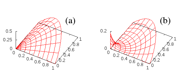
Figure 3: Quasi-corners: (a) $h(r,\varphi)=r\sin\varphi\cos\varphi$; (b) $h(r,\varphi)=(r\log r+1/e)\sin\varphi\cos\varphi$.

For definiteness let us take the basis of the drop at the corner as $\{(x,y)\in[0,\infty)\times[0,\infty)\}$, as on Figs. 3 and use also polar coordinates with $x=r\cos\varphi,\,y=r\sin\varphi$. Let $\mathbf{N}$ denote the normal vector to the fluid surface, which is well defined except at the corner, here the origin. Let $\mathbf{N}_{1}$ be the limit of $\mathbf{N}$ when approaching the origin along the $x$-axis and $\mathbf{N}_{2}$ the limit of $\mathbf{N}$ when approaching the origin along the $y$-axis. For simplicity we take $\mathbf{N}_{1}$ and $\mathbf{N}_{2}$ constant along the corresponding axis, like equilibrium Young angles against two different but homogeneous substrates. Consider a geodesic on the fluid surface going from $(\epsilon,0,0)$ to $(0,\epsilon,0)$ and denote $s$ is the corresponding curvilinear abscissa. On this path

$$\mathbf{N}_{2}-\mathbf{N}_{1}=\int ds\,{\frac{d\mathbf{N}}{ds}}$$ (14)

Assuming the drop surface continuous on the closed domain, including the origin, the total length of the path is less than $2\epsilon$ and thus goes to zero as $\epsilon$ goes to zero, while the left-hand-side is constant. Therefore $d\mathbf{N}/ds$ must go to infinity. If $r\sim\epsilon$ along the geodesic, then $d\mathbf{N}/ds\sim 1/r$. At least one of the principal curvatures is $\mathcal{O}(1/r)$. But the surface is a solution of the Laplace-Young equation, so that the mean curvature is bounded. Therefore the other principal curvature must be also $\mathcal{O}(1/r)$, with opposite sign in order to cancel the divergence as $r\searrow 0$. The radial direction is likely to coincide with the corresponding principal direction, orthogonal or near to the orthogonal to the geodesic. Therefore $d\mathbf{N}/dr\sim 1/r$, or, for each $\varphi$,

$$(1+h^{\prime}(r)^{2})^{-3/2}h^{\prime\prime}(r)\sim 1/r$$ (15)

Taking the primitives on both sides:

$$(1+h^{\prime}(r)^{2})^{-1/2}h^{\prime}(r)\sim\log r+\mathrm{const.}$$ (16)

Hence a contradiction because the left-hand-side is bounded in absolute value by 1 whereas the right-hand-side diverges as $r\searrow 0$. The contradiction can be seen more concretely as follows:

$$h^{\prime}(0)=h^{\prime}(1)-\int_{0}^{1}drh^{\prime\prime}(r)\sim$$

$$h^{\prime}(1)-\int_{0}^{1}dr(1+h{{}^{\prime}}^{2})^{3/2}/r=-\infty,$$ (17)

where (15) was used. This is incompatible with $h\geq 0$ and $h(0)=0$.

We conclude that $\mathbf{t}$ and $\mathbf{n}$ should be continuous all along the contact line, which therefore should be tangent to the $y$-axis at $\pm L/2,\,\pm y_{1},\,\pm y_{2}$ on Fig. 2. And the contact angle itself should be continuous, implying $\theta(\pm L/2)=\theta(\pm y_{1})=\theta_{1}$ and $\theta(\pm y_{2})=\theta_{2}$, forbidding $y_{1}=y_{2}$, as in Fig. 2(c).

Examples of quasi-corners are shown on Fig. 3. They cannot be droplet equilibrium shapes. The surface shown on Fig.  3(a) has mean curvature diverging as $1/r$ as $r\searrow 0$. The surface shown on Fig. 3(b) has principal curvatures diverging as $\pm 1/(r|\log r|^{3})$ as $r\searrow 0$, and mean curvature diverging as $|\log r|$ as $r\searrow 0$. It is not continuous at the origin, and the geodesic used in the argument above has a length $\mathcal{O}(1)$ instead of $\mathcal{O}(\epsilon)$ as $\epsilon\searrow 0$.

3 Molecular dynamics simulation

To study the mechanism behind pinning, we have performed molecular dynamic (MD) simulations of a liquid drop on top of an inclined solid plate ($\alpha=30^{\circ}$ with respect the horizontal) in the proximity of a junction line perpendicular to the inclination. The plate is divided in two half-planes with different wetting properties (more hydrophilic on top of the junction and less hydrophilic below) and subject to a vertical force $\mathbf{F_{0}}$. See Fig. 1. Initially, this external force is equal to zero ($\mathbf{F_{0}}=0$), with the droplet deposited on the more hydrophilic solid and close to the junction. Once the system reaches the equilibrium, defined by a constant energy and a constant value of the local contact angle around the contact line, equal to the equilibrium contact angle, we introduce a force $\mathbf{{F_{0}}\neq 0}$ acting over all the liquid atoms. As a consequence, the liquid drop approaches the junction and the shape of the contact line is altered. Depending on the value of $\mathbf{F_{0}}$, three different scenarii are possible in the simulation: $\left(a\right)$ the base of the drop can be totally on the hydrophilic side of the solid, $\left(b\right)$ part of the contact line can cross over to the hydrophobic solid or $\left(c\right)$ the drop can cross completely the junction and roll over the hydrophobic substrate. We have selected a range of $\mathbf{F_{0}}$ to analyze the three regimes. For each value of $\mathbf{F_{0}}$ used in the simulation, we compute the length of the intersection between the contact line and the junction ($L$) as well as the value of the local contact angles at several points $p_{i}$ along the contact line, $\theta(p_{i})$. Once we have the length $L$ and the contact angles $\theta(p_{i})$, it is possible to compare the simulation results and the new versions of the equilibrium equations obtained through the balance of forces.

3.1 Setup

We consider an incline of angle $\alpha=30^{\circ}$ with respect to the horizontal axis as shown in Fig. 1. The $x$-axis is along the slope downhill, the $y$-axis is horizontal. The upper half-plane ($x<0$) is a relatively hydrophilic substrate $S_{1}$, while the lower half- plane ($x>0$) is a less hydrophilic solid $S_{2}$. The drop profile is $z=h(x,y)$ measured perpendicular to the slope. Close to the $S_{1}/S_{2}$ junction, we put a liquid droplet. An external vertical force $\mathbf{f}_{0}=f_{0}\sin\alpha\mathbf{e}_{x}-f_{0}\cos\alpha\mathbf{e}_{z}$ is acting over each liquid atom and then, the total force acting over the liquid drop is equal to $\mathbf{F}_{0}=N\mathbf{f}_{0}$ where $N$ is the number of liquid atoms that compose the droplet. We denote by $F_{0}$ the modulus of $\mathbf{F}_{0}$ just like $f_{0}$ is the modulus of $\mathbf{f}_{0}.$

Full details of the simulation methods, base parameters and potentials have been given in some previous publications (e.g., Ref. [8, 4] and work cited therein). We recall here the key aspects. The liquids, the solids and their interaction are modeled using Lennard-Jones potentials defined by:

$$V(r_{ij})=4\epsilon C_{AB}\left(\left(\frac{\sigma}{r_{ij}}\right)^{12}-\left(\frac{\sigma}{r_{ij}}\right)^{6}\right)$$ (18)

Here, $r_{ij}$ is the distance between any pair of atoms $i$ and $j$. The coupling parameter $C_{AB}$ enables us to control the relative affinities between the different types of atoms. The parameters $\epsilon$ and $\sigma$ are related, respectively, to the depth of the potential wells and an effective atomic diameter. For both solid and liquid atoms the diameter $\sigma$ is equal to $0.35$ nm, and $\epsilon=k_{B}T$ where $k_{B}$ is the Boltzmann constant and $T=33$ K is the temperature, which is kept constant by a thermostat based on velocity scaling. The pair potential is set to zero for $r_{ij}>2.5\sigma$. $C_{AB}$ is given the value $1$ for both liquid-liquid (LL) and solid-solid (SS) interactions.

$T=33$ K is indeed a very low temperature, because our simulated liquid is a simple toy model liquid. In order to model wetting in molecular dynamics using just Lennard-Jones interactions, we need to work with a system of atoms in a liquid state with a very low viscosity, able to diffuse in short periods of time (of the order of ns). More realistic systems can be considered but the time cost of these simulations will be huge. The chosen parameters for the Lennard-Jones interaction between the linear chains correspond to a liquid system with a low viscosity and low surface tension that allows us to study the wetting dynamic in the scale of few nanoseconds which is reasonable from a computation point of view. This allows us to understand the mechanism behind the physical process and then, use this knowledge in a real system where we expect that the same mechanism will be present. For this particular set of parameters, we have studied drop spreading, [8, 4], capillary bridges, [5], [10], wetting of nanofibers, [27], and in all cases the behaviour of the simulated liquids mimic well what we can measure in the laboratory. Then, we consider that a common mechanism is shared between both systems, the real one and the molecular dynamics simulation. Of course, realistic simulations can be done to model a specific liquid, but more complex interactions must be added with effective parameters measured experimentally. From a fundamental point of view, it is thus easier to work with the simpler system that has the phenomena that one wants to study.

The solid plate is constructed as $66102$ atoms distributed in a rectangular, square-planar lattice having three atomic layers whose normal is parallel to the $z$ axis. The distance between nearest-neighbor solid atoms is set to $2^{1/6}\sigma$ ($0.393$ nm), i.e., the equilibrium distance given by the Lennard-Jones potential. The atoms can vibrate around their initial equilibrium positions according to a harmonic potential defined by $V_{H}(r)=k|\mathbf{r}-\mathbf{r_{0}}|^{2}$ where $k=1000\epsilon/\sigma^{2}$, $\mathbf{r}$ is the instantaneous position of a given solid atom and $\mathbf{r_{0}}$ its initial position. The plane $x=0$ splits the solid plate into two half-planes that we use to model the two solid phases characterized by two different solid-liquid couplings: $C_{LS_{1}}=0.8$ for the hydrophilic substrate $S_{1}$ which corresponds to a Young angle $\theta_{1}=72^{\circ}$, while $C_{LS_{2}}=0.4$ is set for the less hydrophilic solid corresponding to a Young angle $\theta_{2}=135^{\circ}>\theta_{1}$. Then, the value of the local contact angle along the contact line of a drop trapped between the $S_{1}/S_{2}$ junction will be contained in the interval $[72^{\circ},135^{\circ}]$ which allows a large window of analysis.

The liquid is modeled as $5000$ of $8$-atom molecular chains ($N=40000$ atoms), with adjacent atoms linked by a confining potential $U_{\text{conf}}(r_{ij})=Ar_{ij}^{6}$ where $A$ is set to $\epsilon/\sigma^{6}$. This chain length reduces considerably the evaporation (the vapor phase is effectively here vacuum) and allows to use more efficiently all the considered molecules to study pinning over the time scale of the simulation. The masses of all the atoms are equated to that of carbon ($12$ g/mol) to allow comparison with physical systems.

The dimensions of the simulation box are $L_{x}=L_{y}=L_{z}=70$ nm and we impose periodical boundary conditions in the $x$ and $y$ directions. A sketch of the simulation geometry is shown in Fig. 1.

Table 1 shows the values for the external force per atom, $f_{0}$, the total force $F_{0}$ and the corresponding Bond number associated to this force, $Bo=F_{0}R^{2}/(V\gamma)$, where $V$ is the volume of the liquid drop and $R$ is the radius of the initial circular contact line, [21]. The range of the Bond numbers showed in this table are similar to the ones measured by other authors in experiments on the shape and motion of millimetre-size drops of silicon oil sliding down over an homogeneous plane [18] and of glycerol-water mixtures over a substrate decorated with linear chemical steps [26].

$f_{0}$ ($\times 10^{-3}$ pN)	$F_{0}=Nf_{0}$ (pN)	$Bo$
$0.17$	$6.64$	0.12
$0.50$	$19.92$	0.36
$0.83$	$33.21$	0.61
$11.62$	$46.48$	0.85
$16.61$	$66.41$	1.22
$19.93$	$79.69$	1.46
$24.91$	$99.62$	1.82

Table 1: Conversion between simulation units and real units for the external vertical force, and corresponding Bond number.

In a first step, the molecules of the liquid are distributed in a spherical region on top of the solid $S_{1}$ and far from the $S_{1}/S_{2}$ junction meanwhile the temperature of the liquid and the solid is kept constant by rescaling the atoms velocities. After $10^{6}$ time steps, the system reaches the equilibrium characterized by a stable value of the energy and a constant contact angle $\theta_{1}=(70\pm 3)^{\circ}$ along the contact line defined by the intersection between the liquid, the solid $S_{1}$ and the vacuum. Then, we introduce an external vertical force $\mathbf{f}_{0}$ acting over all liquid atoms to model a liquid drop. Depending on the magnitude of this force, the drop can be stuck completely on top of the $S_{1}$ solid or it can get pinned in the $S_{1}/S_{2}$ interface where there appears a segment of length $L$ as the intersection between the contact line and the junction. As a third possibility, the liquid drop can cross completely the junction and roll-off over the $S_{2}$ solid. These three possible behaviors have been observed in our simulations when the value for the total external force was varied from $6$ (drop stuck inside $S_{1}$) to $100$ pN (the limit where the drop rolls off over $S_{2}$). We therefore select a range of $F_{0}$ between these two limits, $F_{0}=6.6$, $19.9$, $33.2$, $46.5$, $66.4$, $79.7$ and $99.6$ pN. For each value of this force we restart the simulation from the previous equilibrated configuration and we let the system evolve during $5\times 10^{6}$ time steps, time long enough to reach a stationary regime characterized by the fluctuation of the energy and the local contact angles around constant values. After that, we run an additional $5\times 10^{6}$ time steps where we decompose the liquid in cubic cells with side $0.1$ nm to calculate the average density inside each cell every $10^{6}$ time steps to have $5$ independent density computations for each value of $F_{0}$ that we will use to compute the average values and their errors for the different magnitudes calculated in this work.

During the application of the external force, the thermostat for scaling of the velocities is only applied to the solid atoms but the collisions between the solid and the liquid atoms are enough to maintain constant the liquid temperature.

3.2 Contact line and intersection length $L$

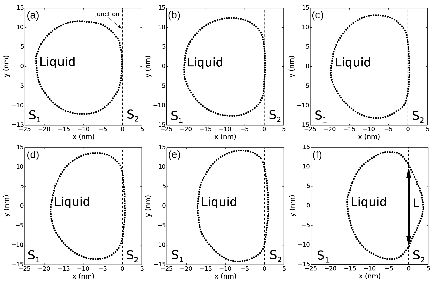
Figure 4: Averaged contact line for (a) $F_{0}=6.6$ pN, (b) $F_{0}=33.2$ pN, (c) $F_{0}=46.5$ pN, (d) $F_{0}=66.4$ pN, (e) $F_{0}=79.7$ pN and (f) $F_{0}=99.6$ pN. The dashed line located at $x=0$ represents the location of the $S_{1}/S_{2}$ junction.

To extract the position of the contact line, it is necessary firstly to determine the location of the liquid-vacuum ($L/V$) interface that we define as the locus where the liquid density is $50\%$ of the density of the liquid in the bulk (i.e. the equimolar surface). To measure the local distribution of this density, we subdivide the available volume of the drop into cubic cells of size $dx$, $dy$, $dz=0.3$ nm and calculate the average number of atoms per cell over $500$ configurations at intervals of $10^{3}$ time steps to extract $10$ independent density profiles, which we use to establish the location of the interface, the position of the contact-line, the local contact angles, and the associated errors. Then, the drop is sliced into $k$ layers parallel to the $L/S$ interface. The density in each slice depends on the $x$-$y$ coordinates, so we decompose the slice into bins perpendicular to the $x$ axis and calculate the density profile along the $y$ coordinate. Finally, this profile is split into two symmetrical regions about the $x$ axis and we fit sigmoidal functions to determine the position of the interface where the density falls to half that of the bulk. This is done for each slice in the $z$ direction to locate the complete liquid-vacuum interface. The contact line is obtained from the intersection between the $L/V$ interface and the solid plate. Fig. 4 shows the different equilibrium contact lines for each value of $F_{0}$ used in this work.

Fig. 4(a)(b)(c) clearly corresponds to Fig. 2(a). Fig. 4(f) clearly corresponds to Fig. 2(c). Fig. 4(d)(e) may correspond to Fig. 2(b). The question is the depth of the protuberance into the hydrophobic side (of order $2$ nm in the MD simulation) and the tentative $y_{1}y_{2}$ segment (of length also a few nanometers): do these lengths scale with the size of the drop or remain of the order of the fluctuations independently of the drop size?

Once the contact line is determined, we compute the intersection between the contact line and the $S_{1}/S_{2}$ junction located at $x=0$. For this, we first locate the two pairs of consecutive points of the contact line that lie on opposite sides with respect to the junction. Then, we determine the two intersections between the two straight lines defined by each one of these pairs of points and the junction. From the distance between these two intersection points we obtain the length of the segment $L$ shown in Fig. 5, the values of which are presented in Table 2.

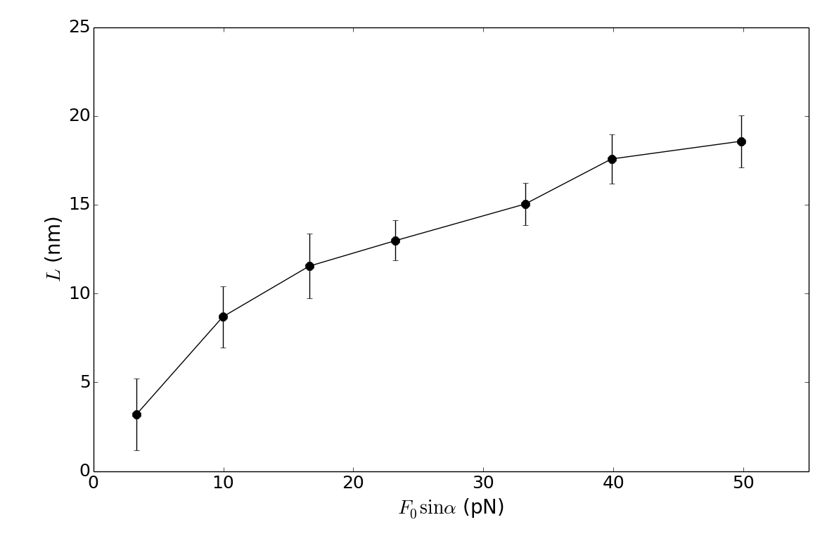
Figure 5: Length $L$ of the segment defined as the intersection between the contact line and the junction, versus $F_{0}\sin\alpha$.

3.3 Contact angles

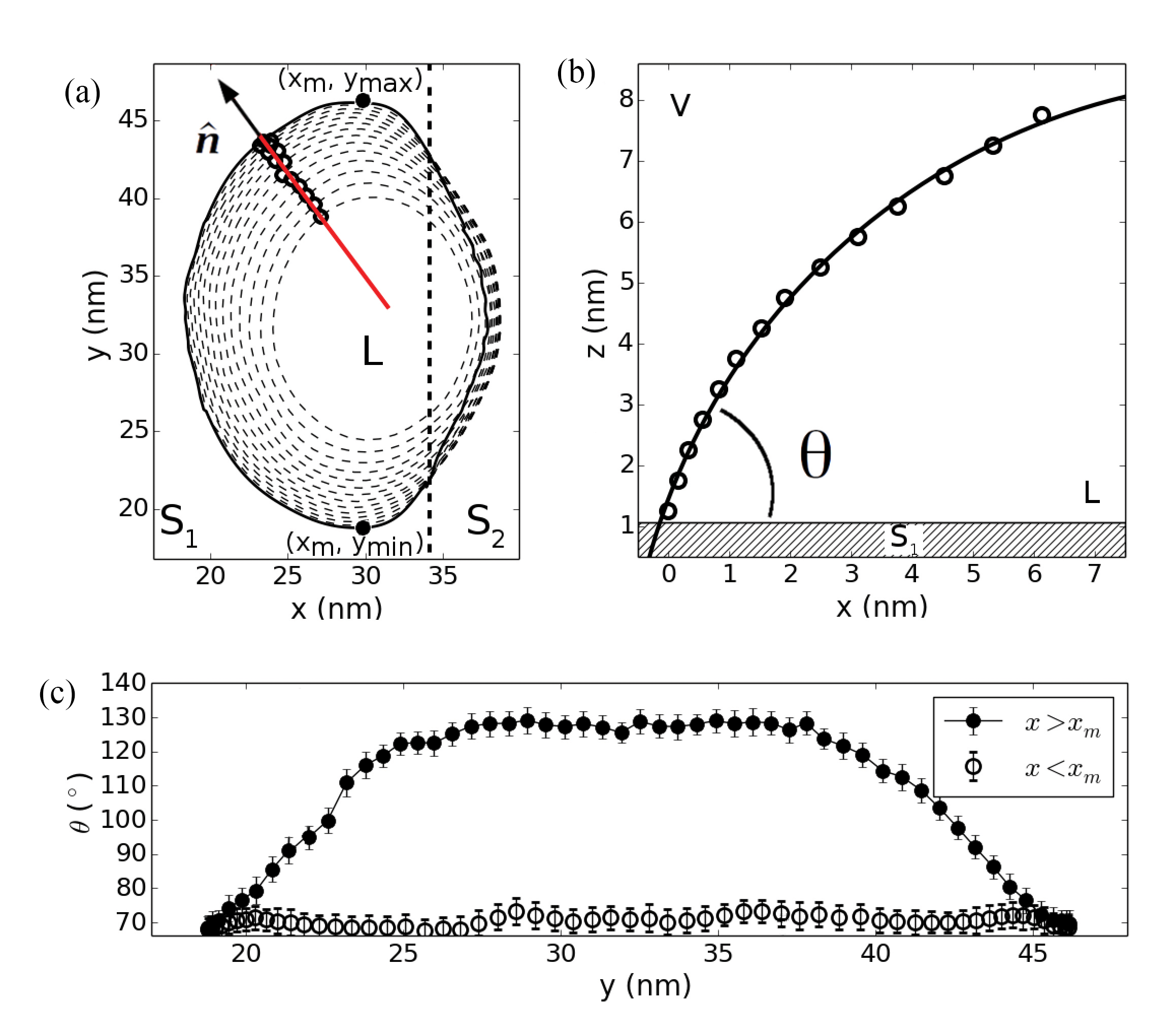
Figure 6: (a) Calculation of the L/V profile at a given point of the contact line. The extremes of the contact line along the $y$-axis are located at $x=x_{m}$. (b) L/V profile and circular fitting used to obtain the local contact angle. (c) Local contact angle versus $y$ for $x<x_{m}$ (open symbols) and $z>x_{m}$ (full symbols). All figures correspond to $F_{0}=99.6$ pN.

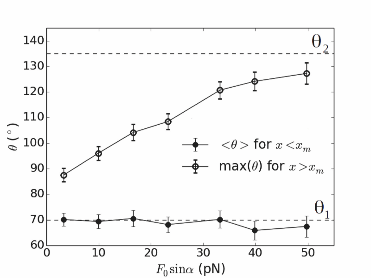
Figure 7: Average value of the local contact angle for $x<x_{m}$, and maximum of local contact angle along the contact line for $x>x_{m}$, versus $F_{0}\sin\alpha$.

For the computation of the local contact angles, we calculate the normal to the contact line in each one of the points of this contact line. Then, we compute the intersection of translates of this normal line with the $L/V$ interface at different heights $z$ as it is sketched in Fig. 6(a). This gives us the profile associated to each point $p_{i}$ of the contact line. We fit a circular arc to this profile and from the slope of this fitted circle at its intersection with the solid we compute the local contact angle at the point $p_{i}$, $\theta(p_{i})$, as it is shown in Fig. 6(b). The extremes in $y$ along the contact line are located at $x=x_{m}$, $y=\pm y_{m}$; we use this to split the contact line in two sets of points for which $x>x_{m}$ and $x<x_{m}$.

Fig. 6(c) shows an example of the dependence of the local contact angle with the $y$ coordinate for $x<x_{m}$ and $x>x_{m}$ for $F_{0}=99.6$ pN. The contact line points at $x<x_{m}$ are located on top of the solid $S_{1}$ and they exhibit a constant contact angle equal to $\theta_{1}$, i.e., to the equilibrium contact angle between this liquid and $S_{1}$. However, for $x>x_{m}$ the contact angle depends on $y$ and varies between $\theta_{1}$ and a maximum value $\theta_{\max}$. As the external force is increased, $\theta_{\max}$ also increases until it reaches the maximum value $\theta_{\max}=\theta_{2}$, as can be seen in Table 2. The average value of the contact angle for $x<x_{m}$ and its maximum value for $x>x_{m}$ are shown in Fig. 7.

In cases (b)(c), $\theta_{\max}=\theta_{2}$ while in case (a), $\theta_{\max}$ depends upon the Bond number and is significantly less than $\theta_{2}$ in agreement with the data in Fig. 7 and Fig. 8 for $F_{0}\sin\alpha<30$ pN.

As can easily be observed in Fig. 7, when the applied force is small enough, we do observe a significant difference between $\theta_{2}$ and $\theta_{\max}$. This is due to the fact that the corresponding contact line is in the vicinity of the $S_{1}/S_{2}$ junction, leading to a clear modification of the density of the liquid in contact with the solid. Indeed, we do observe an increase of the density $\rho_{S_{2}}$ of the liquid able to cross the $S_{1}/S_{2}$ junction, as $F_{0}$ is increased until it reaches the characteristic density of the liquid deposited on top of an homogeneous $S_{2}$ solid ($\rho_{S_{2}}^{0}=21.4$ atoms/nm³). This can be seen in Table 2 where $\rho_{S_{2}}<\rho_{S_{2}}^{0}$ and $\theta_{\max}<\theta_{2}$.

$F_{0}\sin\alpha$ (pN)	$\theta_{\max}$ (∘)	$L$ (nm)	$\rho_{S_{2}}$(atoms/nm3)
$3.32$	87.5	3.6	0.6
$9.96$	96.1	9.7	3.4
$16.61$	104.1	12.8	6.9
$23.24$	108.4	14.4	11.1
$33.21$	120.7	16.7	18.0
$39.85$	124.1	19.5	19.6
$49.81$	127.2	20.2	20.1

Table 2: $\theta_{\max}$, $L$ and density of the first layer of liquid on top of the solid $S_{2}$ for the different values of the external force $F_{0}$ considered in this work. The value of this density if the liquid is totally immersed in $S_{2}$ (no $S_{1}$/$S_{2}$ junction) is $\rho_{S_{2}}^{0}=21.4$ atoms/nm³.

4 Comparison between simulation results and model

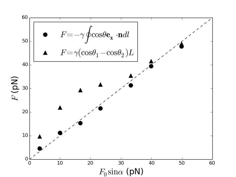
Figure 8: Modulus $F$ of downhill component of capillary force upon drop, versus downhill component $F_{0}\sin\alpha$ of volume (weight) force. Circles: numerical integration of Eq. (3) projected onto the $x$-axis, corresponding to Eq. (5). Triangles: heuristic formula in terms of wetted length $L$ of junction line, corresponding to Eq. (13). The dashed line represents the function $F=F_{0}\sin\alpha$.

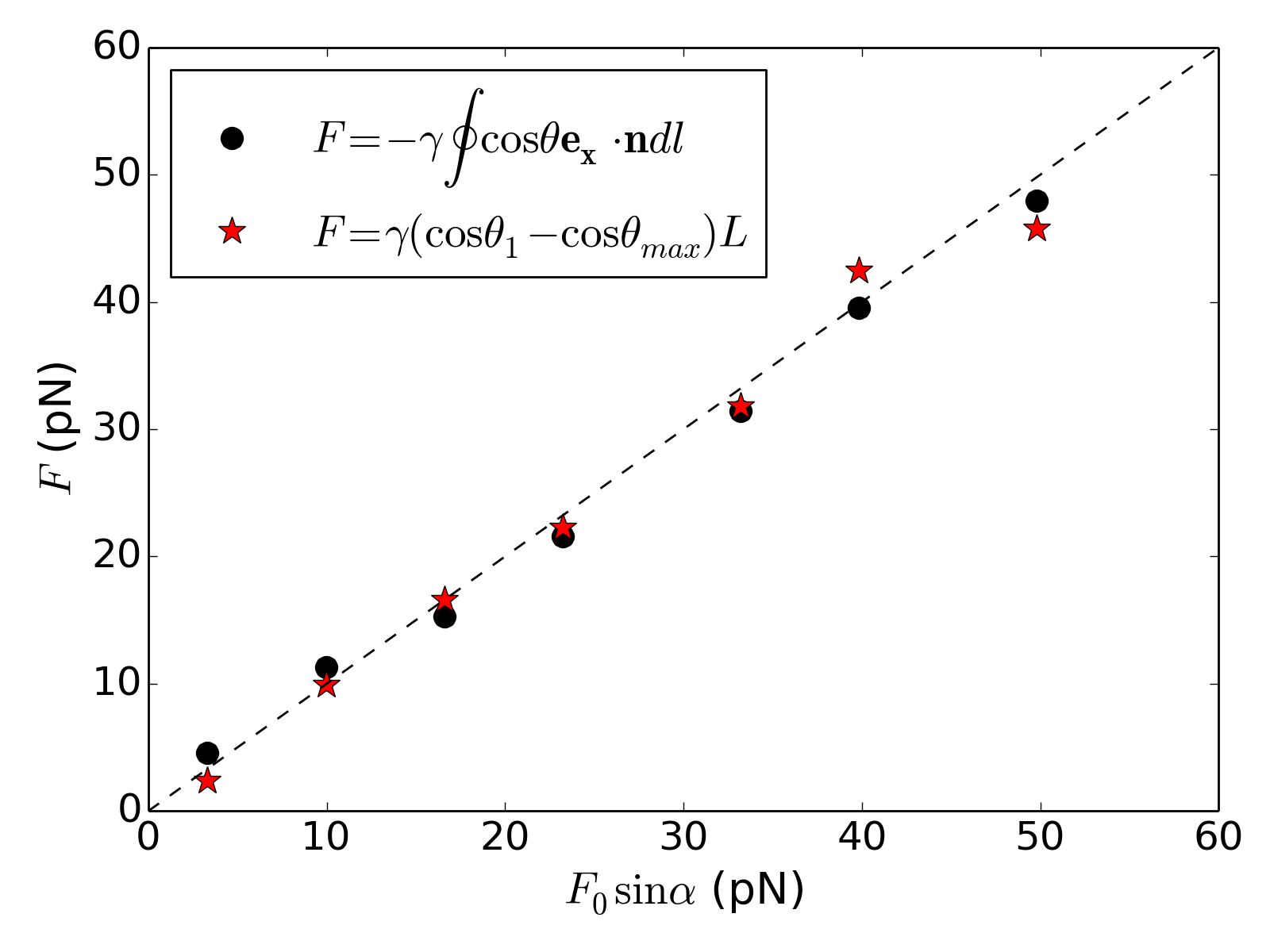
Figure 9: Modulus $F$ of downhill component of capillary force upon drop, versus downhill component $F_{0}\sin\alpha$ of volume (weight) force. Circles: same as in Fig. 8. Stars: heuristic formula in terms of wetted length $L$ of junction line, using the maximum $\theta_{max}$ of the contact angle along the contact line, approximating Eq. (9).

Once we have measured the distribution of the local contact angle along the contact line, it is possible to check the force balance parallel to the Solid-Liquid interface, as given by Eq. (5). To do so, we compute numerically the integral appearing in the modulus $F=-\gamma\,\oint_{\partial\Omega}\,dl\,\mathbf{n}\cdot\mathbf{e_{x}}\,\cos\theta$ of the downhill component of capillary force upon the drop, using a simple trapezoidal method. In practice, we select a set of points around the contact line where we compute the value of the local contact angle $\theta$ and the term $\mathbf{n}\cdot\mathbf{e_{x}}$ inside the contour integral. Fig. 8 shows $F$ versus $F_{0}\sin\alpha$, the downhill component of volume (weight) force. We observe a very good agreement between the simulation results and the model in the full range. Therefore, it is clear that the general Eq. (5) can be used to determine the total force parallel to the Solid-Liquid interface knowing a distribution of points along the contact line and the local contact angle on these points for any value of the external force.

The limitation of the system size in our MD simulations will inevitably affect the amplitude of the contact line fluctuations. It will therefore be difficult to identify case Fig. 2(b) and distinguish it from the end of case Fig. 2(a) or the beginning of case Fig. 2(c). When the value of $F_{0}$ is high enough to reach the unstable configuration sketched in Fig. 2(c), it is possible to use the simplified equation $L\gamma(\cos\theta_{1}-\cos\theta_{2})$ (Eq. (13)) where the only needed parameters are the liquid-vapor surface tension ($\gamma$), the length of the intersection of the contact line with the junction ($L$) and the values of the Young angles of the liquid deposited on top of each one of the solids ($\theta_{1}$ and $\theta_{2}$). Fig. 8 shows that this simple model agrees remarkably well for values of $F_{0}\sin\alpha\gtrsim 33$ pN which corresponds to the system represented in Fig. 4(d), (e) and (f) with $F_{0}\gtrsim 66$ pN. Here the advancing contact angle approaches the Young angle of the liquid on the more hydrophobic solid $S_{2}$ as it can be seen in Fig. 7 and then, we are in the situation sketched in Fig. 2(c) where Eq. (13) should hold. Finally, in Fig. 9, it is shown that in the range $F_{0}\sin\alpha\lesssim 33$ pN, corresponding to the situations sketched in Fig. 4(a), (b) and (c) with $F_{0}\lesssim 66$ pN, it is possible to use the simplified equation $L\gamma(\cos\theta_{1}-\cos\theta_{\max})$ involving the maximum value $\theta_{\max}$ of the contact angle of the drop along the contact line. Concerning Fig. 9 in the thermodynamic limit, the formula for the black circles is exact while the formula for the red stars comes from the approximation $\theta=\theta_{\max}$ all along the part of the contact line with $x\geq 0$. Concerning Fig. 8, the formula for the black triangles is exact in case (c) where $F_{0}\sin\alpha>80$ (not shown on the figure), assuming local equilibrium at any point on the contact line.

5 Conclusion

We have studied a drop pinned on an incline at the junction between a hydrophilic half-plane and a hydrophobic one. In spite of the discontinuity of the $S/L$ surface tension at the junction, we have shown that the contact line must remain a differentiable curve. Based on the equilibrium equations derived from the balance of forces, we have described theoretically three different scenarii: (a) one for which the contact line partly follows the junction line on a segment of width $L$, (b) one for which part of the contact line goes into the hydrophobic half-plane in a central protuberance while keeping two side overlaps with the junction line and (c) one for which part of the contact line crosses straight into the hydrophobic half-plane (See Fig. 2).

In all three cases, we find a formula in the spirit of Furmidge formula Eq. (2), namely:

$$mg\sin\alpha\simeq\gamma\,L\,(\cos\theta_{1}-\cos\theta_{\max}),$$ (19)

where $L$ is the wetted length of the junction line and $\theta_{\max}$ is the maximum of the contact angle along the contact line, which is also the contact angle at the front of the drop. In case (a): $\theta_{\max}<\theta_{2}$ and $\theta_{\max}$ depends upon the Bond number. In cases (b)(c): $\theta_{\max}=\theta_{2}$.

To check the validity of the exact formula (5) and the approximate formula (19), we have performed molecular dynamics simulations for different values of the gravity force $F_{0}=mg.$ We then extracted the local contact angle along the contact line as well as the length $L$ of the contact line intersection with the junction. Then, we have used them to verify the exact full force balance given by Eq. (5) showing excellent agreement. We also checked MD simulation results against the approximate formula (19) in a wide range of $F_{0}=mg$ showing again an excellent agreement. We find a range of small $F_{0}$ where scenario (a) is observed and $\theta_{\max}<\theta_{2}$, then a medium range of $F_{0}$ where scenario (b) is observed and $\theta_{\max}$ slightly smaller than $\theta_{2}$ and a range of larger $F_{0}$ where scenario (c) is observed and $\theta_{\max}=\theta_{2}$.

Acknowledgement. This research was partially funded by the Inter-University Attraction Poles Programme (IAP 7/38 MicroMAST) of the Belgian Science Policy Office. The authors also thank FNRS and RW for partial support. Computational resources have been provided by the Consortium des Equipements de Calcul Intensif (CECI), funded by the Fonds de la Recherche Scientifique de Belgique (F.R.S.-FNRS) under Grant No. 2.5020.11.

References

- [1] V. Berejnov, R. E. Thorne: Effect of transient pinning on stability of drops sitting on an inclined plane. Phys. Rev. E 75, 066308 (2007).
- [2] J. Berthier: Microdrops and digital microfluidics, p.125. Elsevier, second edition (2013).
- [3] J. Berthier, K. Brakke: The physics of microdroplets, p.106. Scrivener-Wiley (2012).
- [4] E. Bertrand, T. D. Blake, and J. De Coninck: Influence of solid-liquid interactions on dynamic wetting: A molecular dynamics study. J. Phys.: Condens. Matter 21, 46124 (2009).
- [5] T. D. Blake, J. C. Fernández-Toledano, G. Doyen, and J. De Coninck: Forced wetting and hydrodynamic assist. Physics of Fluids, 27(11), 112101, (2015).
- [6] R. A. Brown, F.M. Orr Jr., and L. E. Scriven: Static drop on an inclined plate: analysis by the finite element method. Journal Colloid Interface Science 73, 76-87, (1980).
- [7] S. Das, A. Marchand, B. Andreotti, and J. H. Snoeijer: Elastic deformation due to tangential capillary forces. Phys. Fluids 23, 072006 (2011).
- [8] J. De Coninck, T. D. Blake: Wetting and molecular-dynamics simulations of simple liquids. Annu. Rev. Mater. Res. 38, 1-22 (2008).
- [9] J. De Coninck, F. Dunlop, and Th. Huillet: Contact angles of a drop pinned on an incline. Phys. Rev. E, 95(5), 052805 (2017).
- [10] J. C. Fernández-Toledano, T. D. Blake, P. Lambert, and J. De Coninck: On the cohesion of fluids and their adhesion to solids: Young’s equation at the atomic scale. Adv. Colloid Interface Sci. 245, 102-107 (2017).
- [11] P.-G. de Gennes, F. Brochard-Wyart, and D. Quéré: Capillarity and Wetting Phenomena: Drops, Bubbles, Pearls, Waves. Springer-Verlag (2003).
- [12] A. I. ElSherbini, A. M. Jacobi: Liquid drops on vertical and inclined surfaces I. An experimental study of drop geometry. Colloid Interface Sci. 273, 556 (2004).
- [13] A. I. ElSherbini, A. M. Jacobi: Retention forces and contact angles for critical liquid drops on non-horizontal surfaces. Colloid Interface Sci. 299, 841 (2006).
- [14] C. G. L. Furmidge: Studies at Phase Interfaces. Journal of Colloid Science, Vol. 17, No. 4, 309-324, (1962).
- [15] S. J. Gregg: Hysteresis of the contact angle. Chem. Phys. 16, 549 (1948).
- [16] J. F. Joanny, P. G. J. de Gennes: A model for contact angle hysteresis. Chem. Phys. 81, 552 (1984).
- [17] R. E. Johnson, R. H. J. Dettre: Contact angle hysteresis. Phys. Chem. 68, 1744-1750 (1964).
- [18] N. Le Grand, A. Daer and L. Limat: Shape and motion of drops sliding down an inclined plane. J. Fluid Mech. 541, 293-315 (2005).
- [19] N. Moumen, Subramanian R.S., J. McLMaughlin: Experiment on the motion of drops on a horizontal solid surface due to a wettability gradient. Langmuir 22, pp. 2682-2690, 2006.
- [20] T. Podgorski, J.-M. Flesselles, and L. Limat: Corners, cusps and pearls in running drops. Phys. Rev. Lett. 87, 036102-036105, 2001.
- [21] S.W. Rienstra: The shape of a sessile drop for small and large surface tension. Journal of Engineering Mathematics, Vol. 24, No. 3, 193-202, (1990).
- [22] M. J. Santos, S. Velasco, and J. A. White: Simulation analysis of contact angles and retention forces of liquid drops on inclined surfaces. Langmuir, 28(32), 11819-11826, (2012).
- [23] L. W. Schwartz , S. Garoff: Contact angle hysteresis on heterogeneous surfaces. Langmuir. 1, 219 (1985).
- [24] C. Semprebon, M. Brinkmann: On the onset of motion of sliding drops. Soft Matter. 14, 10(18), 3325-34, (2014).
- [25] C. Semprebon, S. Varagnolo, D. Filippi, L. Perlini, M. Pierno, M. Brinkmann, and G. Mistura: Deviation of sliding drops at a chemical step. Soft Matter, 12(40), 8268-8273 (2016).
- [26] C. Semprebon, S. Varagnolo, D. Filippi, L. Perlini, M. Pierno, M. Brinkmann and G. Mistura: Deviation of viscous drops at chemical steps. Soft Matter. 12, 8268-8273 (2016).
- [27] D. Seveno, T. D, Blake, and J. De Coninck: Young’s equation at the nanoscale. Phys. Rev. Lett. 111, 1-4 (2013).
- [28] J. A. White, M. J. Santos, M. A. Rodríguez-Valverde, and S. Velasco: Numerical Study of the Most Stable Contact Angle of Drops on Tilted Surfaces. Langmuir 31, 5326-5332 (2015).
- [29] G. D. Yarnold: The hysteresis of the angle of mercury. Proc. Phys. Soc. 58, 120 (1946).
- [30] T. Young: An Essay on the Cohesion of Fluids. Philos. Trans. R. Soc. Lond. 95, 65 (1805).