Unified convergence analysis of numerical schemes for a miscible displacement problem

Abstract.

This article performs a unified convergence analysis of a variety of numerical methods for a model of the miscible displacement of one incompressible fluid by another through a porous medium. The unified analysis is enabled through the framework of the gradient discretisation method for diffusion operators on generic grids. We use it to establish a novel convergence result in $L^{\infty}(0,T;L^{2}(\Omega))$ of the approximate concentration using minimal regularity assumptions on the solution to the continuous problem. The convection term in the concentration equation is discretised using a centred scheme. We present a variety of numerical tests from the literature, as well as a novel analytical test case. The performance of two schemes are compared on these tests; both are poor in the case of variable viscosity, small diffusion and medium to small time steps. We show that upstreaming is not a good option to recover stable and accurate solutions, and we propose a correction to recover stable and accurate schemes for all time steps and all ranges of diffusion.

1. Introduction

1.1. The miscible displacement model

The single-phase, miscible displacement of one incompressible fluid by another through a porous medium is described by a nonlinearly-coupled initial-boundary value problem [13, 55, 59]. Denote the porous medium by $\Omega$ and write $(0,T)$ for the time period over which the displacement occurs. Neglecting density variations of the mixture within the domain, the unknowns are the hydraulic head $p$ (simply called “pressure” in this paper) and the concentration $c$ of one of the components in the mixture, from which one computes the Darcy velocity $\mathbf{u}$ of the fluid mixture. The model reads

$$\left.\begin{aligned} &\mathbf{u}(x,t)=-\frac{\mathbf{K}(x)}{\mu(c(x,t))}\nabla p(x,t)\\ &\operatorname{div}\mathbf{u}(x,t)=(q^{I}-q^{P})(x,t)\end{aligned}\right\},\quad(x,t)\in\Omega\times(0,T);$$ (1.1a)

$$\Phi(x)\partial_{t}c(x,t)-\operatorname{div}\left(\mathbf{D}(x,\mathbf{u}(x,t))\nabla c-c\mathbf{u}\right)(x,t)=(\hat{c}q^{I}-cq^{P})(x,t),\quad(x,t)\in\Omega\times(0,T).$$ (1.1b)

The reservoir-dependent quantities of porosity and absolute permeability are $$\Phi \mathbf{K} \mathbf{D}(x,\mathbf{u}) \hat{c} q^{I} q^{P}$$ and , respectively. The coefficient is the diffusion-dispersion tensor, and the coefficient is the injected concentration. The sums of injection well source terms and production well sink terms are and , respectively. Assuming that the reservoir boundary is impermeable gives the no-flow boundary conditions

$$\mathbf{u}(x,t)\cdot\mathbf{n}(x) =0,\quad(x,t)\in\partial\Omega\times(0,T),\mbox{ and}$$ (1.1c)

$$\mathbf{D}(x,\mathbf{u})\nabla c(x,t)\cdot\mathbf{n}(x) =0,\quad(x,t)\in\partial\Omega\times(0,T),$$ (1.1d)

where $$\mathbf{n}(x) \partial\Omega x\in\partial\Omega$$ denotes the exterior unit normal to at . The first of these enforces a compatibility condition upon the source terms:

$$\int_{\Omega}q^{I}(x,t)\,\mathrm{d}x=\int_{\Omega}q^{P}(x,t)\,\mathrm{d}x\quad\mbox{for all $t\in(0,T)$.}$$ (1.1e)

One prescribes the initial concentration

$$c(x,0)=c_{0}(x),\quad x\in\Omega,$$ (1.1f)

and the system is completed with a normalisation condition on the pressure to eliminate arbitrary constants in the solution $$p$$ to (1.1a):

$$\int_{\Omega}p(x,t)\,\mathrm{d}x=0\quad\mbox{for all $t\in(0,T)$.}$$ (1.1g)

Russell and Wheeler [59] give a complete derivation of the system (1.1), which is hereafter called the miscible displacement model.

1.2. Literature review

The novelty of this article’s main result — Theorem 3.7 — is twofold. It presents what we believe is the first unified convergence analysis of a number of numerical schemes for the approximation of solutions to (1.1), and it provides a uniform-in-time strong-in-space convergence property for the concentration. The unified analysis is performed using a generic framework which, given a classical numerical method (a list of which is given below) for linear elliptic equations, provides a way to design from it a numerical scheme for the miscible displacement problem that ensures convergence. The uniform-in-time convergence analysis uses a recently-discovered technique [26] developed for scalar degenerate parabolic equations to establish convergence in $L^{\infty}(0,T;L^{2}(\Omega))$ (i.e. uniform-in-time) of the approximate concentrations, thereby improving upon previous results that establish convergence in $L^{2}(0,T;L^{2}(\Omega))$ [4, 56] or in $L^{q}(0,T;L^{r}(\Omega))$ for all $q<\infty$ and $r<2$ [10].

The miscible displacement model has a large and diverse numerical literature [47]. Early work by Peaceman [53, 54] and Douglas [21, 22] uses finite differences. Finite element (FE) and mixed finite element (MFE) methods for the miscible displacement problem were the subject of considerable interest in the $1980$s, with several studies conducted by Douglas, Ewing, Russell, Wheeler and their colleagues [20, 36, 38, 39, 59].

In general, different methods for (1.1a) and (1.1b) are combined to produce a scheme for (1.1). Indeed, the convection-dominated nature of (1.1b) leads Russell and others to develop characteristic tracking methods for handling this equation [37, 57, 58]. Related to these are the so-called Eulerian-Lagrangian localised adjoint methods (ELLAMs) [9, 61]. Finite volume (FV) and mixed finite volume (MFV) methods have been studied for the transport equation alone [2] (with a MFE method for the pressure equation) and the whole system [10], and also Discrete Duality Finite Volume (DDFV) methods [11, 12]. Discontinuous Galerkin (dG) methods are also often employed in the numerical study of (1.1) [4, 50, 56, 60, 62].

1.3. Motivation and framework for the analysis

Given the diversity of methods applied to (1.1) and their corresponding convergences, a natural question to ask is whether we can unify these analyses so that a single convergence proof holds for all (or at least some) of the methods. A unified convergence analysis of this nature requires an appropriate framework; one that is sufficiently abstract so as to encompass as many numerical methods as possible, but sufficiently concrete to recover existing results for the methods in question. Such a framework is the Gradient Discretisation Method (GDM), introduced and developed by Droniou, Eymard, Gallouët, Guichard, Herbin and their collaborators, and which is the subject of a forthcoming monograph [28] to which we refer frequently.

Section 3 gives a reasonably self-contained presentation of the elements of the GDM required for the subsequent analysis of (1.1). Following the GDM literature, it identifies the four key properties of coercivity, consistency, limit-conformity and compactness that a numerical method must satisfy in order for the subsequent proof of Theorem 3.7 in Section 5 to apply. If a numerical method can be written in such a manner that it satisfies these four properties, then Theorem 3.7 shows that it will approximate solutions to (1.1) with convergences prescribed in the statement of the theorem. In particular, the approximate concentrations will converge in $L^{\infty}(0,T;L^{2}(\Omega))$.

At the time of writing, methods known to satisfy the GDM framework include FE with mass lumping [15]; the Crouzeix-Raviart non-conforming FE, with or without mass-lumping [17, 35]; the Raviart–Thomas MFE [7]; the Discontinuous Galerkin scheme in its Symmetric Interior Penalty version [19]; the Multi-Point Flux Approximation (MPFA) O-method [1, 34]; DDFV methods in dimension two [3, 49] and the CeVeFE–DDFV scheme in dimension three [16]; the Hybrid Mimetic Mixed (HMM) family [29], which includes the SUSHI scheme [42], Mixed Finite Volumes [25] and mixed-hybrid Mimetic Finite Differences (MFD) [8]; nodal MFD [6]; and the Vertex Approximate Gradient (VAG) scheme [43]. Theorem 3.7 therefore applies to these methods, when a centred discretisation is employed for the convection term.

For most nonlinear models, convergence proofs using the GDM framework are based on compactness techniques. In contrast to establishing error estimates on the solution — the method favoured by most studies in the literature cited above — such analyses do not require uniqueness or regularity of the solution to the continuous problem, assumptions that are inconsistent with what the physical problem suggests and what the theory provides (see the discussion in Droniou, Eymard and Herbin [31]). The cost of removing these uniqueness/regularity assumptions is the ability to establish rates of convergence with respect to discretisation parameters. Examples of studies that employ compactness techniques include Chainais-Hillairet–Droniou (MFV) [10]; Amaziane and Ossmani (MFE/FV) [2]; Bartels, Jensen and Müller (dG) [4]; Rivière and Walkington (dG/MFE) [56] and subsequently Li, Rivière and Walkington [50] (dG).

Compactness techniques first establish a priori energy estimates on the solution to the numerical scheme, which yield weak compactness in the appropriate spaces. Ensuring convergence of the numerical solutions for nonlinear problems such as (1.1b) typically requires stronger compactness than what the estimates alone afford. For time-dependent problems, one obtains such compactness by estimating the temporal variation of the numerical solution. From here one may apply discrete analogues of the Aubin–Simon lemma.

This is the procedure we employ herein. Our estimates on the discrete pressure and concentration are a straightforward adaptation of Chainais-Hillairet–Droniou [10]. The discrete time derivative estimate Lemma 4.4 is in the spirit of Droniou–Eymard–Gallouët–Herbin [30], and for the convergence of the scheme we adapt many arguments from Eymard–Gallouët–Guichard–Masson [41], who study a related two-phase flow problem.

1.4. Centred discretisation of the convection term

The GDM framework offers a generic discretisation of diffusion operators, but (1.1) features a (dominant) convection term $\operatorname{div}(c\mathbf{u})$. This term is usually discretised with an upstream weighted scheme, or occasionally the aforementioned modified method of characteristics. The motivation for our use of a centred discretisation is that it is an opportunity to compare the upstream and centred approaches by the results of numerical experiments conducted using two simple schemes that we present in Section 3.2. The numerical results provided in Section 6 include test cases from the literature, as well as a novel analytical test case. As expected, they show that both schemes are well-behaved in the presence of sufficient diffusion. With small dispersion and the absence of molecular diffusion, centred schemes also behave rather well for time steps of the same magnitude as those commonly used in the literature. However, they display large instabilities for smaller time steps, and upstream versions similarly do not produce acceptable results. We propose a way to introduce in centred schemes some additional diffusion to recover accurate and stable results for a wide range of time steps. This diffusion is isotropic, scaled by the magnitude of the Darcy velocity, and vanishes with the mesh size.

Constructing a centred scheme is straightforward in the GDM framework. We mention however that including other kinds of advection discretisations in a unified analysis is possible, by following the ideas of Beirão da Veiga, Droniou and Manzini [5] for HMM methods (or other face-based methods), and Eymard, Feron and Guichard in the context of incompressible Navier–Stokes [40].

Let us finally remark that, to enable the convergence analysis, we apply a truncation (onto the unit interval) to the concentration in the convection term, and we add a boundedness hypothesis on $\mathbf{D}$ to remove the truncation from the limit equation (see Remark 5.1).

1.5. Notation

For a topological vector space $X(\Omega)$ of functions on $\Omega$, we write $(X(\Omega))^{\prime}$ for its topological dual. When writing the duality pairing $\langle\cdot,\cdot\rangle_{(X(\Omega))^{\prime},X(\Omega)}$, we omit the subscripts if they are clear from the context.

When $z\in(1,\infty)$ is a Lebesgue/Sobolev exponent, we write $z^{\prime}=\frac{z}{z-1}$ for its conjugate. We denote by $H_{\star}^{1}(\Omega)$ those elements of $H^{1}(\Omega)$ whose integral over $\Omega$ vanishes, equipped with the usual norms.

We use $C$ to denote an arbitrary positive constant that may change from line to line. When $C$ appears in an estimate we track only its relevant dependencies (or non-dependencies, as is frequently the case). These dependencies are understood to be nondecreasing.

Given $x\in\Omega$ and $\zeta\in{\mathbb{R}}^{d}$, we write $\mathbf{D}^{1/2}(x,\zeta)$ for the square root of $\mathbf{D}(x,\zeta)$, which is well defined since we always assume that $\mathbf{D}(x,\zeta)$ is a symmetric, positive-definite matrix; similarly for $\mathbf{A}$ and $\mathbf{A}^{1/2}$ defined in the next section.

2. Problem reformulation and assumptions

In order to simplify the presentation, we write the miscible displacement model in the following synthesised form, henceforth using $(\overline{p},\overline{\mathbf{u}},\overline{c})$ to denote exact solutions and $(p,\mathbf{u},c)$ to denote approximate solutions obtained by the numerical scheme:

$$\left.\begin{aligned} &\operatorname{div}(\overline{\mathbf{u}})=q^{I}-q^{P}\quad\mbox{in $\Omega\times(0,T)$,}&\qquad&\overline{\mathbf{u}}=-\mathbf{A}(\cdot,\overline{c})\nabla\overline{p}\quad\mbox{in $\Omega\times(0,T)$,}\\ &\int_{\Omega}\overline{p}(x,\cdot)\,\mathrm{d}x=0\quad\mbox{on $(0,T)$,}&\qquad&\overline{\mathbf{u}}\cdot\mathbf{n}=0\quad\mbox{on $\partial\Omega\times(0,T)$,}\end{aligned}\right\}$$ (2.1a)

$$\left.\begin{aligned} &\Phi\partial_{t}\overline{c}-\operatorname{div}(\mathbf{D}(\cdot,\overline{\mathbf{u}})\nabla\overline{c})+\operatorname{div}(\overline{c}\,\overline{\mathbf{u}})=\hat{c}q^{I}-\overline{c}q^{P}\quad\mbox{in $\Omega\times(0,T)$,}\\ &\overline{c}(\cdot,0)=c_{0}\quad\mbox{in $\Omega$,}\\ &\mathbf{D}(\cdot,\overline{\mathbf{u}})\nabla\overline{c}\cdot\mathbf{n}=0\quad\mbox{on $\partial\Omega\times(0,T)$.}\end{aligned}\right\}$$ (2.1b)

Our assumptions on the data are then as follows.

$$\begin{array}[]{c}\Omega\mbox{ is a bounded, connected {polytopal} subset of ${\mathbb{R}}^{d}$, $d=1,2$ or $3$, and $T>0$.}\end{array}$$ (2.2a)

Denote by $$\mathcal{S}_{d}({\mathbb{R}}) d\times d \mathbf{A} \mathbf{K} \mu$$ the set of symmetric matrices with real entries. The tensor encodes the absolute permeability and viscosity :

$$\begin{array}[]{c}\mathbf{A}:\Omega\times{\mathbb{R}}\to\mathcal{S}_{d}({\mathbb{R}})\mbox{ is a Carath\'{e}odory function such that}\\ \exists\alpha_{\mathbf{A}}>0,\,\exists\Lambda_{\mathbf{A}}>0\mbox{ such that, for a.e. $x\in\Omega$, all $s\in{\mathbb{R}}$ and all $\xi\in{\mathbb{R}}^{d}$,}\\ \mathbf{A}(x,s)\xi\cdot\xi\geq\alpha_{\mathbf{A}}|\xi|^{2}\mbox{ and }|\mathbf{A}(x,s)|\leq\Lambda_{\mathbf{A}}.\end{array}$$ (2.2b)

We assume that the diffusion-dispersion tensor satisfies

$$\begin{array}[]{c}\mathbf{D}:\Omega\times{\mathbb{R}}^{d}\to\mathcal{S}_{d}({\mathbb{R}})\mbox{ is a Carath\'{e}odory function such that}\\ \exists\alpha_{\mathbf{D}}>0,\,\exists\Lambda_{\mathbf{D}}>0\mbox{ such that, for a.e. $x\in\Omega$ and all }\zeta,\xi\in{\mathbb{R}}^{d},\\ \mathbf{D}(x,\zeta)\xi\cdot\xi\geq\alpha_{\mathbf{D}}|\xi|^{2}\mbox{ and }|\mathbf{D}(x,\zeta)|\leq\Lambda_{\mathbf{D}}.\end{array}$$ (2.2c)

The assumptions on the porosity, injected concentration and initial concentration are standard:

$$\begin{array}[]{c}\Phi\in L^{\infty}(\Omega)\mbox{ and there exists }\phi_{\ast}>0\mbox{ such that for a.e. $x\in\Omega$, }\phi_{\ast}\leq\Phi(x)\leq\phi_{\ast}^{-1};\end{array}$$ (2.2d)

$$\begin{array}[]{c}\hat{c}\in L^{\infty}(\Omega\times(0,T))\mbox{ satisfies }0\leq\hat{c}(x,t)\leq 1\mbox{ for a.e. }(x,t)\in\Omega\times(0,T);\end{array}$$ (2.2e)

$$\begin{array}[]{c}c_{0}\in L^{\infty}(\Omega)\mbox{ satisfies }0\leq c_{0}(x)\leq 1\mbox{ for a.e. }x\in\Omega.\end{array}$$ (2.2f)

Finally, we assume that

$$\begin{array}[]{c}q^{I},q^{P}\in L^{\infty}(\Omega\times(0,T))\mbox{ are nonnegative and such that }\\ \int_{\Omega}q^{I}(x,\cdot)\,\mathrm{d}x=\int_{\Omega}q^{P}(x,\cdot)\,\mathrm{d}x\mbox{ a.e. in }(0,T).\end{array}$$ (2.2g)

Remark 2.1.

Peaceman showed [53] that the diffusion-dispersion tensor takes the form

$$\mathbf{D}(x,\mathbf{u})=\Phi(x)\bigg{(}d_{m}\mathbf{I}+|\mathbf{u}|\Big{(}d_{l}\mathbf{E}(\mathbf{u})+d_{t}(\mathbf{I}-\mathbf{E}(\mathbf{u}))\Big{)}\bigg{)},\quad\mbox{with}\quad\mathbf{E}(\mathbf{u})=\left(\frac{\mathbf{u}_{i}\mathbf{u}_{j}}{|\mathbf{u}|^{2}}\right)_{1\leq i,j\leq d}.$$ (2.3)

Here $\mathbf{I}$ is the $d$-dimensional identity matrix, $d_{m}>0$ is the molecular diffusion coefficient, and $d_{l}>0$ and $d_{t}>0$ are the longitudinal and transverse mechanical dispersion coefficients, respectively.

Although (2.3) satisfies the coercivity condition in (2.2c), it is not uniformly bounded. Indeed, one can show that $|\mathbf{D}(x,\mathbf{u})|\leq C(1+|\mathbf{u}|)$, where $C>0$. The necessity of our stronger assumption on $\mathbf{D}$ can be traced to our choice of discretisation for the convection term in (2.1b); we discuss this further below.

We henceforth supress the dependence on space of $\mathbf{A}$ and $\mathbf{D}$ from the notation by writing $\mathbf{A}(x,c)=\mathbf{A}(c)$ and $\mathbf{D}(x,\mathbf{u})=\mathbf{D}(\mathbf{u})$.

Remark 2.2.

The assumption that the sources are bounded is primarily to simplify the analysis. Indeed, it suffices to take $q^{I}\in L^{\infty}(0,T;L^{2}(\Omega))$ and $q^{P}\in L^{\infty}(0,T;L^{r}(\Omega))$, where $r>1$ if $d=2$ and $r\geq\frac{3}{2}$ if $d=3$. These spatial regularities on $q^{P}$ arise from the need to bound the production well term in the discrete time derivative estimate (4.11) below, which can be accomplished using a discrete Sobolev inequality [28, Lemma B.24]. Employing this inequality, one can improve the spatial regularity of both the discrete test function and the approximation to $\overline{c}$ from $L^{2}$ to $L^{q}$ for all $q<\infty$ (if $d=2$) or to $L^{6}$ (if $d=3$). Whilst most of the schemes that we consider in the Gradient Discretisation Method framework satisfy such a discrete Sobolev inequality, its sole usage herein would be in the estimate (4.11).

The main result of this article demonstrates that our approximate solutions converge to the following notion of weak solution to (2.1), the existence of which is due to Feng [46], Chen and Ewing [14] (both of whom assume Peaceman’s diffusion-dispersion tensor) and Fabrie and Gallouët [45] (who use the assumption (2.2c)).

Definition 2.1.

Assume (2.2). A weak solution to (2.1) is a pair of functions $(\overline{p},\overline{c})$ satisfying

$$\left.\begin{gathered}\overline{c}\in L^{2}(0,T;H^{1}(\Omega))\cap C([0,T];L^{2}(\Omega)),\quad 0\leq\overline{c}(x,t)\leq 1\quad\mbox{for a.e. $(x,t)\in\Omega\times(0,T)$;}\\ \Phi\partial_{t}\overline{c}\in L^{2}(0,T;(H^{1}(\Omega))^{\prime}),\quad\overline{c}(\cdot,0)=c_{0}\quad\mbox{in $L^{2}(\Omega)$};\\ \overline{p}\in L^{\infty}(0,T;H^{1}_{\star}(\Omega)),\quad\overline{\mathbf{u}}(x,t)=-\mathbf{A}(\overline{c}(x,t))\nabla\overline{p}(x,t);\\ -\int_{0}^{T}\int_{\Omega}\overline{\mathbf{u}}(x,t)\cdot\nabla\varphi(x,t)\,\mathrm{d}x\,\mathrm{d}t\\ =\int_{0}^{T}\int_{\Omega}\left(q^{I}-q^{P}\right)(x,t)\varphi(x,t)\,\mathrm{d}x\,\mathrm{d}t\quad\forall\varphi\in L^{1}(0,T;H^{1}(\Omega));\\ \int_{0}^{T}\langle\Phi\partial_{t}\overline{c}(\cdot,t),\psi(\cdot,t)\rangle\,\mathrm{d}t+\int_{0}^{T}\int_{\Omega}\mathbf{D}(\overline{\mathbf{u}}(x,t))\nabla\overline{c}(x,t)\cdot\nabla\psi(x,t)\,\mathrm{d}x\,\mathrm{d}t\\ -\int_{0}^{T}\int_{\Omega}\overline{c}(x,t)\,\overline{\mathbf{u}}(x,t)\cdot\nabla\psi(x,t)\,\mathrm{d}x\,\mathrm{d}t\\ =\int_{0}^{T}\int_{\Omega}\left(\hat{c}q^{I}-\overline{c}q^{P}\right)(x,t)\psi(x,t)\,\mathrm{d}x\,\mathrm{d}t,\quad\forall\psi\in L^{2}(0,T;H^{1}(\Omega)).\end{gathered}\right\}$$ (2.4)

There are two noteworthy features to this definition. First, the regularity of $\overline{c}$ matches that of $\varphi$, so one can take $\varphi=\overline{c}$. In doing so, by integrating by parts on the time derivative term and using the elliptic equation to transform the convective term (see the proof of [32, Proposition 3.1]), it is straightforward to show that for every $T_{0}\in(0,T)$, the solution satisfies the identity

$$\begin{gathered}\frac{1}{2}\int_{\Omega}\Phi(x)\left(\overline{c}(x,T_{0})^{2}-c_{0}(x)^{2}\right)\,\mathrm{d}x=\int_{0}^{T_{0}}\int_{\Omega}\left(\overline{c}\hat{c}q^{I}\right)(x,t)\,\mathrm{d}x\,\mathrm{d}t\\ -\frac{1}{2}\int_{0}^{T_{0}}\int_{\Omega}\left(\overline{c}^{2}(q^{I}+q^{P})\right)(x,t)\,\mathrm{d}x\,\mathrm{d}t-\int_{0}^{T_{0}}\int_{\Omega}\mathbf{D}(\overline{\mathbf{u}}(x,t))\nabla\overline{c}(x,t)\cdot\nabla\overline{c}(x,t)\,\mathrm{d}x\,\mathrm{d}t.\end{gathered}$$ (2.5)

We will see that the ability to take $\overline{c}$ as a test function in the transport equation is critical to ensuring our generic discretisations properly approximate (2.4), and this resultant identity enables improved temporal convergence of the approximation to $\overline{c}$.

We consider a solution to be a pair $(\overline{p},\overline{c})$ rather than a triple $(\overline{p},\overline{\mathbf{u}},\overline{c})$. This is inconsequential, and comes from the fact that our generic discretisation below requires only approximations of $\overline{p}$ and $\overline{c}$, from which we obtain an approximation $\overline{\mathbf{u}}$ by the discrete gradient operator. Note however that many finite element and finite volume schemes for (2.1) approximate $\overline{\mathbf{u}}$ directly, since numerical differentiation of the approximation to $\overline{p}$ can lead to rather poor approximations of the Darcy velocity [18, 37].

3. Discrete problem and main result

The basic objects of study in our GDM discretisation of the miscible displacement problem are the gradient discretisation, which must satisfy the four properties of coercivity, consistency, limit-conformity and compactness in order to guarantee convergence of the associated gradient scheme.

3.1. Gradient discretisation

Definition 3.1 (Gradient discretisation).

A gradient discretisation for the miscible displacement problem is a family $\mathcal{D}=(X_{\mathcal{D}},\Pi_{\mathcal{D}},\nabla_{\mathcal{D}},\mathcal{I}_{\mathcal{D}},(t^{(n)})_{n=0,\ldots,N})$, where

1. The set $X_{\mathcal{D}}$ of discrete unknowns is a finite-dimensional vector space over ${\mathbb{R}}$.

2. $\Pi_{\mathcal{D}}:X_{\mathcal{D}}\to L^{2}(\Omega)$ is a linear mapping, called the function reconstruction operator.

3. $\nabla_{\mathcal{D}}:X_{\mathcal{D}}\to L^{2}(\Omega)^{d}$ is a linear mapping called the gradient reconstruction operator, and must be chosen so that $\left\lVert\,\cdot\,\right\rVert_{\mathcal{D},\mathrm{ell}}$ defined by

   $$\left\lVert w\right\rVert_{\mathcal{D},\mathrm{ell}}=\left[\left\lVert\nabla_{\mathcal{D}}w\right\rVert^{2}_{L^{2}(\Omega)^{d}}+\left(\int_{\Omega}\Pi_{\mathcal{D}}w(x)\,\mathrm{d}x\right)^{2}\right]^{1/2}$$

   is a norm on $X_{\mathcal{D}}$. We also define

   $$\left\lVert w\right\rVert_{\mathcal{D},\mathrm{para}}=\left[\left\lVert\Pi_{\mathcal{D}}w\right\rVert^{2}_{L^{2}(\Omega)}+\left\lVert\nabla_{\mathcal{D}}w\right\rVert^{2}_{L^{2}(\Omega)^{d}}\right]^{1/2}.$$

4. $\mathcal{I}_{\mathcal{D}}:L^{2}(\Omega)\to X_{\mathcal{D}}$ is a linear interpolation operator.

5. $0=t^{(0)}<t^{(1)}<\ldots<t^{(N)}=T$.

Note that besides the use of the $\left\lVert\,\cdot\,\right\rVert_{\mathcal{D},\mathrm{para}}$ norm in (iii), this notion of gradient discretisation is identical to the space-time gradient discretisation for parabolic Neumann problems presented in [28, Definitions 3.1 and 4.1].

The subscripts ‘$\mathrm{ell}$’ and ‘$\mathrm{para}$’ denote elliptic and parabolic, respectively, and reflect the fact that we use $\left\lVert\,\cdot\,\right\rVert_{\mathcal{D},\mathrm{ell}}$ to estimate the discrete pressure and $\left\lVert\,\cdot\,\right\rVert_{\mathcal{D},\mathrm{para}}$ to estimate the discrete concentration. The manner in which we incorporate the zero-mean value of the pressure into the scheme (see (3.3a)) necessitates the use of the $\left\lVert\,\cdot\,\right\rVert_{\mathcal{D},\mathrm{ell}}$ norm and its associated Poincaré inequality (3.4) to obtain a spatial $L^{2}$ estimate on the discrete pressure. The presence of the time derivative in the parabolic equation affords the same estimate without the use of a Poincaré inequality, hence the $\left\lVert\,\cdot\,\right\rVert_{\mathcal{D},\mathrm{para}}$ norm.

Next we introduce some notation. Consider $n\in\{0,\ldots,N-1\}$, $t\in(t^{(n)},t^{(n+1)}]$ and $w=(w^{(n)})_{n=0,\ldots,N-1}\in X_{\mathcal{D}}^{N}$. Set $\delta t^{(n+\frac{1}{2})}=t^{(n+1)}-t^{(n)}$, $\delta t_{\mathcal{D}}=\max_{n=0,\ldots,N-1}\delta t^{(n+\frac{1}{2})}$ and define the discrete time derivative

$$\delta_{\mathcal{D}}w(t):=\delta_{\mathcal{D}}^{(n+\frac{1}{2})}w:=\Pi_{\mathcal{D}}\frac{w^{(n+1)}-w^{(n)}}{\delta t^{(n+\frac{1}{2})}}\in L^{2}(\Omega).$$

We use the notation $\Pi_{\mathcal{D}}^{\mathrm{ex}}$, $\Pi_{\mathcal{D}}$, $\nabla_{\mathcal{D}}$ (with ‘exp’ for explicit) for functions dependent on both space and time as follows. For almost-every $x\in\Omega$, for all $n\in\{0,\ldots,N-1\}$ and all $t\in(t^{(n)},t^{(n+1)}]$, we set

$$\begin{gathered}\Pi_{\mathcal{D}}w(x,0)=\Pi_{\mathcal{D}}^{\mathrm{ex}}w(x,0)=\Pi_{\mathcal{D}}w^{(0)}(x),\quad\Pi_{\mathcal{D}}^{\mathrm{ex}}w(x,t)=\Pi_{\mathcal{D}}w^{(n)}(x),\\ \Pi_{\mathcal{D}}w(x,t)=\Pi_{\mathcal{D}}w^{(n+1)}(x),\mbox{ and }\nabla_{\mathcal{D}}w(x,t)=\nabla_{\mathcal{D}}w^{(n+1)}(x).\end{gathered}$$ (3.1)

Normally only one choice of evaluation is required, either implicit ($\Pi_{\mathcal{D}}w(x,t)=\Pi_{\mathcal{D}}w^{(n+1)}(x)$) or explicit ($\Pi_{\mathcal{D}}w(x,t)=\Pi_{\mathcal{D}}w^{(n)}(x))$. Again, the coupled nature of the miscible displacement problem appears to necessitate the use of both. We discuss this further below.

Before introducing the scheme, one final remark is necessary. The solution $\overline{c}$ to (2.1b) satisfies a maximum principle: $0\leq\overline{c}\leq 1$. We cannot in general prove such an a priori estimate on the numerical approximation of $\overline{c}$ in the GDM framework, except in very specific cases such as the two-point finite volume scheme on simple meshes and with a diffusion-dispersion tensor that does not depend on $\mathbf{u}$ [24, 41]. Indeed, in Section 6 we present numerical results on coarse meshes that exhibit values of the concentration outside the unit interval. To establish the basic discrete energy estimates of Lemma 4.2 on the numerical solution, it is therefore necessary for us to stabilise the scheme by means of a truncation operator applied to $\overline{c}$ in the convection term. To this end, for $s\in{\mathbb{R}}$ define the truncation onto the unit interval by

$${\mathbb{T}}(s):=\max(0,\min(s,1)).$$ (3.2)

The scheme for (2.1) is then obtained by replacing the continuous spaces and operators in (2.4) with their discrete analogues.

Definition 3.2 (Gradient scheme for (2.1)).

Find sequences $p=\left(p^{(n)}\right)_{n=1,\ldots,N}\in X_{\mathcal{D}}^{N}$ and $c=\left(c^{(n)}\right)_{n=0,\ldots,N}\in X_{\mathcal{D}}^{N+1}$ such that $c^{(0)}=\mathcal{I}_{\mathcal{D}}c_{0}$ and for all $n=0,\ldots,N-1$,

$$\left.\begin{gathered}\mathbf{u}_{\mathcal{D}}^{(n+1)}(x)=-\mathbf{A}\left(\Pi_{\mathcal{D}}c^{(n)}(x)\right)\nabla_{\mathcal{D}}p^{(n+1)}(x),\\ -\int_{\Omega}\mathbf{u}_{\mathcal{D}}^{(n+1)}(x)\cdot\nabla_{\mathcal{D}}w(x)\,\mathrm{d}x+\left(\int_{\Omega}\Pi_{\mathcal{D}}p^{(n+1)}(x)\,\mathrm{d}x\right)\left(\int_{\Omega}\Pi_{\mathcal{D}}w(x)\,\mathrm{d}x\right)\\ =\frac{1}{\delta t^{(n+\frac{1}{2})}}\int_{t^{(n)}}^{t^{(n+1)}}\int_{\Omega}(q^{I}-q^{P})(x,t)\Pi_{\mathcal{D}}w(x)\,\mathrm{d}x\,\mathrm{d}t\quad\forall w\in X_{\mathcal{D}},\end{gathered}\right\}$$ (3.3a)

$$\begin{gathered}\int_{\Omega}\left(\Phi(x)\delta_{\mathcal{D}}^{(n+\frac{1}{2})}c(x)\Pi_{\mathcal{D}}w(x)+\mathbf{D}(\mathbf{u}_{\mathcal{D}}^{(n+1)}(x))\nabla_{\mathcal{D}}c^{(n+1)}(x)\cdot\nabla_{\mathcal{D}}w(x)\right)\,\mathrm{d}x\\ -\int_{\Omega}{\mathbb{T}}\left(\Pi_{\mathcal{D}}c^{(n+1)}(x)\right)\mathbf{u}_{\mathcal{D}}^{(n+1)}(x)\cdot\nabla_{\mathcal{D}}w(x)\,\mathrm{d}x\\ =\frac{1}{\delta t^{(n+\frac{1}{2})}}\int_{t^{(n)}}^{t^{(n+1)}}\int_{\Omega}\left(\hat{c}(x)q^{I}(x,t)-\Pi_{\mathcal{D}}c^{(n+1)}(x)q^{P}(x,t)\right)\Pi_{\mathcal{D}}w(x)\,\mathrm{d}x\,\mathrm{d}t\quad\forall w\in X_{\mathcal{D}}.\end{gathered}$$ (3.3b)

Note the choice of $\Pi_{\mathcal{D}}c^{(n)}$ (i.e. explicit in time) in the definition of the discrete Darcy velocity. This choice follows Chainais-Hillairet–Droniou [10] and decouples the scheme for (2.1a) from the scheme for (2.1b). This facilitates the proof of existence of solutions to (3.3), but is by no means necessary. It does, however, reflect a structural choice common to many schemes in the literature on the miscible displacement problem. The second integral term in (3.3a) accounts for the zero mean value of $\overline{p}$.

In order to prove the main result of this article, our gradient discretisations must satisfy properties that mimic as much as possible the properties of the continuous operators. The first of these, coercivity, imposes a restriction on the $L^{2}$ interaction between $\Pi_{\mathcal{D}}$ and $\nabla_{\mathcal{D}}$. In particular, it gives us a discrete Poincaré inequality and ensures stability of the underlying method.

Definition 3.3 (Coercivity).

Let

$$C_{\mathcal{D}}=\max_{w\in X_{\mathcal{D}}\setminus\{0\}}\frac{\left\lVert\Pi_{\mathcal{D}}w\right\rVert_{L^{2}(\Omega)}}{\left\lVert w\right\rVert_{\mathcal{D},\mathrm{ell}}}.$$

A sequence $(\mathcal{D}_{m})_{m\in{\mathbb{N}}}$ of gradient discretisations is coercive if there exists $C_{P}\in{\mathbb{R}}^{+}$ such that for all $m\in{\mathbb{N}}$, $C_{\mathcal{D}_{m}}\leq C_{P}$.

The corresponding Poincaré inequality for the $\left\lVert\,\cdot\,\right\rVert_{\mathcal{D},\mathrm{ell}}$ norm is then

$$\left\lVert\Pi_{\mathcal{D}}w\right\rVert_{L^{2}(\Omega)}\leq C_{\mathcal{D}}\left\lVert w\right\rVert_{\mathcal{D},\mathrm{ell}}.$$ (3.4)

The next property, consistency, ensures that we can recover our (spatial) solution space $H^{1}(\Omega)$ to arbitrary $L^{2}$ precision using reconstructed functions and their gradients from $X_{\mathcal{D}}$. In this sense, it shows that $X_{\mathcal{D}}$ is a ‘good sample’ of $H^{1}(\Omega)$. This property also ensures the recovery of the initial condition, and the convergence to 0 of the time steps.

Definition 3.4 (Consistency).

For $\varphi\in H^{1}(\Omega)$, define the map $S_{\mathcal{D}}:H^{1}(\Omega)\to[0,\infty)$ by

$$S_{\mathcal{D}}(\varphi)=\min_{w\in X_{\mathcal{D}}}\left(\left\lVert\Pi_{\mathcal{D}}w-\varphi\right\rVert_{L^{2}(\Omega)}+\left\lVert\nabla_{\mathcal{D}}w-\nabla\varphi\right\rVert_{L^{2}(\Omega)^{d}}\right).$$

A sequence $(\mathcal{D}_{m})_{m\in{\mathbb{N}}}$ of gradient discretisations is consistent if, as $m\to\infty$,

• for all $\varphi\in H^{1}(\Omega)$, $S_{\mathcal{D}_{m}}(\varphi)\to 0$,

• for all $\varphi\in L^{2}(\Omega)$, $\Pi_{\mathcal{D}_{m}}\mathcal{I}_{\mathcal{D}_{m}}\varphi\to\varphi$ strongly in $L^{2}(\Omega)$, and

• $\delta t_{\mathcal{D}_{m}}\to 0$.

Elements of the continuous spaces in our problem satisfy a divergence formula. The quantity $W_{\mathcal{D}}$ defined below measures the error introduced into this formula by the discretisation method. For convergence of the schemes, we require that the formula is satisfied asymptotically.

Definition 3.5 (Limit-conformity).

Let $W=\left\{\bm{\varphi}\in C^{\infty}(\overline{\Omega})^{d}:\bm{\varphi}\cdot\mathbf{n}=0\mbox{ on }\partial\Omega\right\}$. For $\bm{\varphi}\in W$, define $W_{\mathcal{D}}:W\to[0,\infty)$ by

$$W_{\mathcal{D}}(\bm{\varphi})=\max_{w\in X_{\mathcal{D}}\setminus\{0\}}\frac{1}{\left\lVert w\right\rVert_{\mathcal{D},\mathrm{ell}}}\left|\int_{\Omega}\left(\nabla_{\mathcal{D}}w(x)\cdot\bm{\varphi}(x)+\Pi_{\mathcal{D}}w(x)\operatorname{div}\bm{\varphi}(x)\,\mathrm{d}x\right)\right|.$$

A sequence $(\mathcal{D}_{m})_{m\in{\mathbb{N}}}$ of gradient discretisations is limit-conforming if for all $\bm{\varphi}\in W$, $W_{\mathcal{D}_{m}}(\bm{\varphi})\to 0$ as $m\to\infty$. This implies also the same property with $\left\lVert w\right\rVert_{\mathcal{D},\mathrm{para}}$ instead of $\left\lVert w\right\rVert_{\mathcal{D},\mathrm{ell}}$.

The condition of vanishing normal trace in $W$ is imposed by the homogeneous Neumann boundary conditions of the miscible displacement model [28].

Our final requirement on the gradient discretisations is that the operators $\Pi_{\mathcal{D}}$ and $\nabla_{\mathcal{D}}$ afford us a compactness property.

Definition 3.6 (Compactness).

A sequence $(\mathcal{D}_{m})_{m\in{\mathbb{N}}}$ of gradient discretisations is compact if for all sequences $(u_{m})_{m\in{\mathbb{N}}}$ with $u_{m}\in X_{\mathcal{D}_{m}}$ such that $(\left\lVert u_{m}\right\rVert_{\mathcal{D},\mathrm{para}})_{m\in{\mathbb{N}}}$ or $(\left\lVert u_{m}\right\rVert_{\mathcal{D},\mathrm{ell}})_{m\in{\mathbb{N}}}$ is bounded, the sequence $\left(\Pi_{\mathcal{D}_{m}}u_{m}\right)_{m\in{\mathbb{N}}}$ has a subsequence converging in $L^{2}(\Omega)$.

With these definitions in place, the main result of this article is the following theorem.

Theorem 3.7.

Assume (2.2) and let $(\mathcal{D}_{m})_{m\in{\mathbb{N}}}$ be a sequence of gradient discretisations that is coercive, consistent, limit-conforming and compact. For $m\in{\mathbb{N}}$, let $(p_{\mathcal{D}_{m}},c_{\mathcal{D}_{m}})$ be a solution to the gradient scheme (3.3) with $\mathcal{D}=\mathcal{D}_{m}$. Then there exists a weak solution $(\overline{p},\overline{c})$ of (2.1) in the sense of Definition 2.1 and a subsequence of gradient discretisations, again denoted $(\mathcal{D}_{m})_{m\in{\mathbb{N}}}$, such that as $m\to\infty$,

1. $\Pi_{\mathcal{D}_{m}}p_{\mathcal{D}_{m}}\to\overline{p}$ strongly in $L^{p}(0,T;L^{2}(\Omega))$ for every $p<\infty$ and weakly-$\ast$ in $L^{\infty}(0,T;L^{2}(\Omega))$;

2. $\nabla_{\mathcal{D}_{m}}p_{\mathcal{D}_{m}}\to\nabla\overline{p}$ and $\mathbf{u}_{\mathcal{D}_{m}}:=-\mathbf{A}\left(\Pi_{\mathcal{D}_{m}}^{\mathrm{ex}}c_{\mathcal{D}_{m}}\right)\nabla_{\mathcal{D}_{m}}p_{\mathcal{D}_{m}}\to\overline{\mathbf{u}}$, both strongly in $L^{2}(0,T;L^{2}(\Omega)^{d})$;

3. $\Pi_{\mathcal{D}_{m}}c_{\mathcal{D}_{m}}\to\overline{c}$ and $\Pi_{\mathcal{D}_{m}}^{\mathrm{ex}}c_{\mathcal{D}_{m}}\to\overline{c}$ strongly in $L^{\infty}(0,T;L^{2}(\Omega))$;

4. $\nabla_{\mathcal{D}_{m}}c_{\mathcal{D}_{m}}\rightharpoonup\nabla\overline{c}$ weakly in $L^{2}(0,T;L^{2}(\Omega)^{d})$.

3.2. Two examples

We present here two concrete examples that fit into the GDM framework.

3.2.1. Scheme A: finite-difference scheme

Scheme A, defined only on rectangular meshes, leads to a five-point finite volume scheme in the case of isotropic diffusion problems on rectangular meshes. For the sake of simplicity, we describe this scheme in the case where $\Omega=(0,L)^{2}$, with $L>0$. For $N\in{\mathbb{N}}$, set $h=L/N$, and for $i,j=1,\ldots,N$, set $K_{ij}=((i-1)h,ih)\times((j-1)h,jh)$. We then set

1. $X_{\mathcal{D}}=\{(u_{ij})_{i,j=1,\ldots,N}\in{\mathbb{R}}^{N^{2}}\}$;

2. For every $u\in X_{\mathcal{D}}$, $i,j=1,\ldots,N$ and for almost-every $x\in K_{ij}$, $\Pi_{\mathcal{D}}u(x)=u_{ij}$ (piecewise constant reconstruction in all $K_{ij}$);

3. For every $u\in X_{\mathcal{D}}$, for $i,j=1,\ldots,N$, set $u_{N+1,j}=u_{Nj}$, $u_{i,N+1}=u_{iN}$, $u_{0j}=u_{1j}$, and $u_{i0}=u_{i1}$. For $i,j=1,\ldots,N$, we then define the piecewise constant reconstruction of the gradient by

   1. $\nabla_{\mathcal{D}}u(x)=(\frac{1}{h}(u_{i+1,j}-u_{ij}),\frac{1}{h}(u_{i,j+1}-u_{ij}))$ on $((i-\frac{1}{2})h,ih)\times((j-\frac{1}{2})h,jh)$,

   2. $\nabla_{\mathcal{D}}u(x)=(\frac{1}{h}(u_{i+1,j}-u_{ij}),\frac{1}{h}(u_{i,j}-u_{i,j-1}))$ on $((i-\frac{1}{2})h,ih)\times((j-1)h,(j-\frac{1}{2})h)$,

   3. $\nabla_{\mathcal{D}}u(x)=(\frac{1}{h}(u_{ij}-u_{i-1,j}),\frac{1}{h}(u_{i,j+1}-u_{ij}))$ on $((i-1)h,(i-\frac{1}{2})h)\times((j-\frac{1}{2})h,jh)$,

   4. $\nabla_{\mathcal{D}}u(x)=(\frac{1}{h}(u_{ij}-u_{i-1,j}),\frac{1}{h}(u_{i,j}-u_{i,j-1}))$ on $((i-1)h,(i-\frac{1}{2})h)\times((j-1)h,(j-\frac{1}{2})h)$.

   Figure 1 provides a visualisation of this construction.

For proofs that this scheme is coercive, consistent, limit conforming and compact in the case of homogeneous Dirichlet boundary conditions, see Droniou, Eymard and Feron [27]. The adaptation of their arguments to homogeneous Neumann boundary conditions is straightforward.

Figure 1. Discrete gradient for Scheme A

3.2.2. Scheme B: mass-lumped $P^{1}$ conforming scheme

Scheme B, defined only for conforming triangular meshes, is the standard $P^{1}$ conforming finite element scheme with mass lumping on the dual mesh obtained by joining the center of gravity of the triangles with the middle of the edges [28, Section 8.4] (dual meshes can also easily be defined in 3D, so this scheme is actually also defined for 3D simplicial meshes). Denote by $\mathcal{V}$ the set of the vertices of the mesh, and for $i\in\mathcal{V}$ define $K_{i}$ as the dual cell around the vertex $i$. We then set

1. $X_{\mathcal{D}}=\{u=(u_{i})_{i\in\mathcal{V}}\in{\mathbb{R}}^{\mathcal{V}}\}$;

2. For every $u\in X_{\mathcal{D}}$, $i\in\mathcal{V}$ and for almost-every $x\in K_{i}$, $\Pi_{\mathcal{D}}u(x)=u_{i}$ (piecewise constant reconstruction in all $K_{i}$);

3. For every $u\in X_{\mathcal{D}}$, define $\nabla_{\mathcal{D}}u$ as the gradient of the conforming piecewise affine function reconstructed in the triangles from the values at the vertices of the triangles.

For proofs that this scheme satisfies the four properties above in the case of homogeneous Dirichlet boundary conditions, see Droniou, Eymard and Herbin [31]. Their adaptation to homogeneous Neumann boundary conditions is once again straightforward (see also [28, Sections 8.3 and 8.4]).

We revisit these schemes in Section 6 to present the results of numerical experiments.

4. Estimates

Thanks to the gradient discretisation framework, the following elliptic estimates are very similar to their continuous analogues. To reiterate the conventions outlined in the introduction, for the constants appearing in estimates we highlight only their relevant dependencies. In the current setting, this amounts to highlighting scheme-dependent quantities and demonstrating that the additional regularity assumed on the sources really is primarily for convenience.

Lemma 4.1.

Assume (2.2) and let $\mathcal{D}$ be a gradient discretisation. Let $(p,c)$ be a solution to the gradient scheme for (2.1). Then there exists $C$ depending only on $C_{P}\geq C_{\mathcal{D}}$ and $\left\lVert q^{I}-q^{P}\right\rVert_{L^{\infty}(0,T;L^{2}(\Omega))}$ such that

$$\left\lVert\Pi_{\mathcal{D}}p\right\rVert_{L^{\infty}(0,T;L^{2}(\Omega))}\leq C,\quad\left\lVert\nabla_{\mathcal{D}}p\right\rVert_{L^{\infty}(0,T;L^{2}(\Omega)^{d})}\leq C\quad\mbox{and}\quad\left\lVert\mathbf{u}_{\mathcal{D}}\right\rVert_{L^{\infty}(0,T;L^{2}(\Omega)^{d})}\leq C.$$ (4.1)

As a consequence, for a given $n\in\{0,\ldots,N-1\}$, there exists one and only one $p^{(n+1)}\in X_{\mathcal{D}}$ such that (3.3a) holds.

Proof.

Let $n\in\{0,\ldots,N-1\}$ and take $w=p^{(n+1)}$ in (3.3a) to obtain

$$\int_{\Omega}\mathbf{A}\left(\Pi_{\mathcal{D}}c^{(n)}(x)\right)\nabla_{\mathcal{D}}p^{(n+1)}(x)\cdot\nabla_{\mathcal{D}}p^{(n+1)}(x)\,\mathrm{d}x+\left(\int_{\Omega}\Pi_{\mathcal{D}}p^{(n+1)}(x)\,\mathrm{d}x\right)^{2}\\ =\frac{1}{\delta t^{(n+\frac{1}{2})}}\int_{t^{(n)}}^{t^{(n+1)}}\int_{\Omega}\left(q^{I}-q^{P}\right)(x,t)\Pi_{\mathcal{D}}p^{(n+1)}(x)\,\mathrm{d}x\,\mathrm{d}t.$$

Next, apply the coercivity (2.2b) of $\mathbf{A}$ and Hölder’s inequality:

$$\alpha_{\mathbf{A}}\int_{\Omega}\left|\nabla_{\mathcal{D}}p^{(n+1)}(x)\right|^{2}\,\mathrm{d}x+\left(\int_{\Omega}\Pi_{\mathcal{D}}p^{(n+1)}(x)\,\mathrm{d}x\right)^{2}\leq\left\lVert q^{I}-q^{P}\right\rVert_{L^{\infty}(0,T;L^{2}(\Omega))}\left\lVert\Pi_{\mathcal{D}}p^{(n+1)}\right\rVert_{L^{2}(\Omega)}.$$

Then using the discrete Poincaré inequality (3.4), we have

$$\int_{\Omega}\left|\nabla_{\mathcal{D}}p^{(n+1)}(x)\right|^{2}\,\mathrm{d}x+\left(\int_{\Omega}\Pi_{\mathcal{D}}p^{(n+1)}(x)\,\mathrm{d}x\right)^{2}\leq\left(\frac{C_{\mathcal{D}}}{\min(1,\alpha_{\mathbf{A}})}\right)^{2}\left\lVert q^{I}-q^{P}\right\rVert_{L^{\infty}(0,T;L^{2}(\Omega))}^{2}.$$ (4.2)

This yields the estimate on $\nabla_{\mathcal{D}}p$ and, thanks again to (3.4), the estimate on $\Pi_{\mathcal{D}}p$. The estimate on $\mathbf{u}_{\mathcal{D}}$ follows from the estimate on $\nabla_{\mathcal{D}}p$ and the bound on $\mathbf{A}$.

For a given $n\in\{0,\ldots,N-1\}$, (3.3a) is a square linear system. If the right-hand side of (3.3a) vanishes, (4.2) shows that the system has a trivial kernel. The existence and uniqueness of the solution $p^{(n+1)}\in X_{\mathcal{D}}$ to (3.3a) then follows immediately. ∎

The following discrete energy estimates are also a reasonably straightforward translation of the continous estimates [32, Proposition 3.1]. Note however that unlike the continuous estimates, due to our use of the truncation operator we cannot follow [45] by using the pressure equation to transform the convection term.

Lemma 4.2.

Assume (2.2) and let $\mathcal{D}$ be a gradient discretisation. Let $(p,c)$ be a solution to the gradient scheme for (2.1). Then there exists $C$ depending only on $C_{P}\geq C_{\mathcal{D}}$, $\left\lVert q^{I}\right\rVert_{L^{\infty}(0,T;L^{2}(\Omega))}$, $\left\lVert q^{P}\right\rVert_{L^{\infty}(0,T;L^{2}(\Omega))}$ and $C_{I}\geq\left\lVert\Pi_{\mathcal{D}}c^{(0)}\right\rVert_{L^{2}(\Omega)}$ such that

$$\left\lVert\Pi_{\mathcal{D}}c\right\rVert_{L^{\infty}(0,T;L^{2}(\Omega))}\leq C,\quad\left\lVert\Pi_{\mathcal{D}}^{\mathrm{ex}}c\right\rVert_{L^{\infty}(0,T;L^{2}(\Omega))}\leq C\quad\mbox{and}\quad\left\lVert\nabla_{\mathcal{D}}c\right\rVert_{L^{2}(0,T;L^{2}(\Omega)^{d})}\leq C.$$ (4.3)

Proof.

Take $n\in\{0,\ldots,N-1\}$ and $w=c^{(n+1)}$ in (3.3b) to obtain

$$\int_{\Omega}\left(\Phi(x)\delta_{\mathcal{D}}^{(n+\frac{1}{2})}c(x)\Pi_{\mathcal{D}}c^{(n+1)}(x)+\mathbf{D}(\mathbf{u}_{\mathcal{D}}^{(n+1)}(x))\nabla_{\mathcal{D}}c^{(n+1)}(x)\cdot\nabla_{\mathcal{D}}c^{(n+1)}(x)\right)\,\mathrm{d}x\\ -\int_{\Omega}{\mathbb{T}}\left(\Pi_{\mathcal{D}}c^{(n+1)}(x)\right)\mathbf{u}_{\mathcal{D}}^{(n+1)}(x)\cdot\nabla_{\mathcal{D}}c^{(n+1)}(x)\,\mathrm{d}x+\frac{1}{\delta t^{(n+\frac{1}{2})}}\int_{t^{(n)}}^{t^{(n+1)}}\int_{\Omega}\left(\Pi_{\mathcal{D}}c^{(n+1)}(x)\right)^{2}q^{P}(x,t)\,\mathrm{d}x\,\mathrm{d}t\\ =\frac{1}{\delta t^{(n+\frac{1}{2})}}\int_{t^{(n)}}^{t^{(n+1)}}\int_{\Omega}\hat{c}(x,t)q^{I}(x,t)\Pi_{\mathcal{D}}c^{(n+1)}(x)\,\mathrm{d}x\,\mathrm{d}t.$$ (4.4)

For $a$, $b\in{\mathbb{R}}$, $(a-b)a=\frac{1}{2}(a^{2}-b^{2})+\frac{1}{2}(a-b)^{2}$. Applying this to the discrete time derivative term yields

$$\left(\Pi_{\mathcal{D}}c^{(n+1)}-\Pi_{\mathcal{D}}c^{(n)}\right)\Pi_{\mathcal{D}}c^{(n+1)}={} \frac{1}{2}\left((\Pi_{\mathcal{D}}c^{(n+1)})^{2}-(\Pi_{\mathcal{D}}c^{(n)})^{2}\right)$$ (4.5)

$${+\frac{1}{2}\left(\Pi_{\mathcal{D}}c^{(n+1)}-\Pi_{\mathcal{D}}c^{(n)}\right)^{2}}.$$

Then multiplying (4.4) by $\delta t^{(n+\frac{1}{2})}$ and summing over $n=0,\ldots,m-1$ for some $m\in[1,N]$, we have

$$\frac{1}{2}\int_{\Omega}\Phi(x)\left[\left(\Pi_{\mathcal{D}}c^{(m)}(x)\right)^{2}-\left(\Pi_{\mathcal{D}}c^{(0)}(x)\right)^{2}\right]\,\mathrm{d}x+\int_{0}^{t^{(m)}}\int_{\Omega}\mathbf{D}(\mathbf{u}_{\mathcal{D}}(x,t))\nabla_{\mathcal{D}}c(x,t)\cdot\nabla_{\mathcal{D}}c(x,t)\,\mathrm{d}x\,\mathrm{d}t\\ -\int_{0}^{t^{(m)}}\int_{\Omega}{\mathbb{T}}\left(\Pi_{\mathcal{D}}c(x,t)\right)\mathbf{u}_{\mathcal{D}}(x,t)\cdot\nabla_{\mathcal{D}}c(x,t)\,\mathrm{d}x\,\mathrm{d}t+\int_{0}^{t^{(m)}}\int_{\Omega}\left(\Pi_{\mathcal{D}}c(x,t)\right)^{2}q^{P}(x,t)\,\mathrm{d}x\,\mathrm{d}t\\ \leq\int_{0}^{t^{(m)}}\int_{\Omega}\hat{c}(x,t)q^{I}(x,t)\Pi_{\mathcal{D}}c(x,t)\,\mathrm{d}x\,\mathrm{d}t.$$ (4.6)

One estimates the diffusion-dispersion term from below using the coercivity (2.2c). Thanks to the nonnegativty of $q^{P}$, the last term on the left-hand side is nonnegative. Applying Young’s inequality with $\varepsilon=\alpha_{\mathbf{D}}$ to the convection term, we obtain

$$\frac{1}{2}\int_{\Omega}\Phi(x)\left[\left(\Pi_{\mathcal{D}}c^{(m)}(x)\right)^{2}-\left(\Pi_{\mathcal{D}}c^{(0)}(x)\right)^{2}\right]\,\mathrm{d}x+\frac{\alpha_{\mathbf{D}}}{2}\int_{0}^{t^{(m)}}\int_{\Omega}\left|\nabla_{\mathcal{D}}c(x,t)\right|^{2}\,\mathrm{d}x\,\mathrm{d}t\\ \leq T\left\lVert q^{I}\right\rVert_{L^{\infty}(0,T;L^{2}(\Omega))}\left\lVert\Pi_{\mathcal{D}}c\right\rVert_{L^{\infty}(0,T;L^{2}(\Omega))}+\frac{T}{2\alpha_{\mathbf{D}}}\left\lVert\mathbf{u}_{\mathcal{D}}\right\rVert_{L^{\infty}(0,T;L^{2}(\Omega))}^{2}.$$ (4.7)

In particular, using the estimate (4.1) on $\mathbf{u}_{\mathcal{D}}$ and again applying Young’s inequality with $\varepsilon=\frac{\phi_{\ast}}{2T}$,

$$\frac{\phi_{\ast}}{2}\int_{\Omega}\left(\Pi_{\mathcal{D}}c^{(m)}(x)\right)^{2}\,\mathrm{d}x\\ \leq\frac{1}{2\phi_{\ast}}\left\lVert\Pi_{\mathcal{D}}c^{(0)}\right\rVert_{L^{2}(\Omega)}^{2}+\frac{\phi_{\ast}}{4}\left\lVert\Pi_{\mathcal{D}}c\right\rVert_{L^{\infty}(0,T;L^{2}(\Omega))}^{2}+\frac{T^{2}}{\phi_{\ast}}\left\lVert q^{I}\right\rVert_{L^{\infty}(0,T;L^{2}(\Omega))}^{2}+\frac{TC^{2}}{2\alpha_{\mathbf{D}}}.$$

The right-hand side of this inequality does not depend on $m$. Since

$$\left\lVert\Pi_{\mathcal{D}}c\right\rVert_{L^{\infty}(0,T;L^{2}(\Omega))}^{2}=\sup_{m=1,\ldots,N}\int_{\Omega}\left(\Pi_{\mathcal{D}}c^{(m)}(x)\right)^{2}\,\mathrm{d}x,$$

this yields the estimate on $\left\lVert\Pi_{\mathcal{D}}c\right\rVert_{L^{\infty}(0,T;L^{2}(\Omega))}$. The estimate on $\left\lVert\Pi_{\mathcal{D}}^{\mathrm{ex}}c\right\rVert_{L^{\infty}(0,T;L^{2}(\Omega))}$ follows from the fact that $\left\lVert\Pi_{\mathcal{D}}^{\mathrm{ex}}c\right\rVert_{L^{\infty}(0,T;L^{2}(\Omega))}=\max(\left\lVert\Pi_{\mathcal{D}}c\right\rVert_{L^{\infty}(0,T;L^{2}(\Omega))},\left\lVert\Pi_{\mathcal{D}}c^{(0)}\right\rVert_{L^{2}(\Omega)})$. Revisiting (4.7) gives the estimate on $\nabla_{\mathcal{D}}c$. ∎

The nonlinearity introduced by the truncation operator necessitates the use of a fixed point argument to confirm the existence of solutions to the scheme.

Corollary 4.3.

Assume (2.2) and let $\mathcal{D}$ be a gradient discretisation. Then there exists at least one solution $(p,c)$ to the gradient scheme of Definition 3.2.

Proof.

Take $n\in\{0,\ldots,N-1\}$ and assume that $(p^{(n)},c^{(n)})$ are given. Lemma 4.1 gives the existence of the solution $p^{(n+1)}$ to (3.3a). It remains to demonstrate the existence of a solution $c^{(n+1)}$ to (3.3b). Define $F:X_{\mathcal{D}}\to X_{\mathcal{D}}$, where for $z\in X_{\mathcal{D}}$, $v=F(z)$ is the solution to

$$\begin{gathered}\int_{\Omega}\left(\Phi(x)\Pi_{\mathcal{D}}\frac{v-c^{(n)}}{\delta t^{(n+\frac{1}{2})}}(x)\Pi_{\mathcal{D}}w(x)+\mathbf{D}(\mathbf{u}_{\mathcal{D}}^{(n+1)}(x))\nabla_{\mathcal{D}}v(x)\cdot\nabla_{\mathcal{D}}w(x)\right)\,\mathrm{d}x\\ -\int_{\Omega}{\mathbb{T}}(\Pi_{\mathcal{D}}z(x))\mathbf{u}_{\mathcal{D}}^{(n+1)}(x)\cdot\nabla_{\mathcal{D}}w(x)\,\mathrm{d}x=\frac{1}{\delta t^{(n+\frac{1}{2})}}\int_{t^{(n)}}^{t^{(n+1)}}\int_{\Omega}\hat{c}(x)q^{I}(x,t)\Pi_{\mathcal{D}}w(x)\,\mathrm{d}x\,\mathrm{d}t\\ -\frac{1}{\delta t^{(n+\frac{1}{2})}}\int_{t^{(n)}}^{t^{(n+1)}}\int_{\Omega}\Pi_{\mathcal{D}}v(x)q^{P}(x,t)\Pi_{\mathcal{D}}w(x)\,\mathrm{d}x\,\mathrm{d}t\quad\forall w\in X_{\mathcal{D}}.\end{gathered}$$

Replacing $c^{(n+1)}$ by $z$ does not change the computations of Lemma 4.2. This shows the existence of $C$ not depending on $z$ such that $\left\lVert\Pi_{\mathcal{D}}v\right\rVert_{L^{2}(\Omega)}\leq C$ and $\left\lVert\nabla_{\mathcal{D}}v\right\rVert_{L^{2}(\Omega)^{d}}\leq C$. Since $F$ is continuous, apply Brouwer’s fixed point theorem to conclude. ∎

In order to obtain the required level of compactness, we must estimate the so-called discrete time derivative. For this we require an appropriate dual norm. To this end, define $B_{\mathcal{D}}=\left\{\Pi_{\mathcal{D}}v\,|\,v\in X_{\mathcal{D}}\right\}\subset L^{2}(\Omega)$, and equip it with the norms

$$\left\lVert u\right\rVert_{B_{\mathcal{D}}}=\inf\left\{\left\lVert v\right\rVert_{\mathcal{D},\mathrm{para}}:v\in X_{\mathcal{D}}\mbox{ is such that }u=\Pi_{\mathcal{D}}v\right\}\mbox{ and}$$ (4.8)

$$\left\lVert u\right\rVert_{\ast,B_{\mathcal{D}}}=\sup\left\{\int_{\Omega}\Phi(x)u(x)\Pi_{\mathcal{D}}w(x)\,\mathrm{d}x:w\in X_{\mathcal{D}},\,\left\lVert w\right\rVert_{\mathcal{D},\mathrm{para}}=1\right\}.$$ (4.9)

Note that $\left\lVert\cdot\right\rVert_{*,B_{\mathcal{D}}}$ is indeed a norm [28, Section 4.2.1], and that

$$\forall u\in B_{\mathcal{D}}\,,\;\forall w\in X_{\mathcal{D}}\,,\;\left|\int_{\Omega}\Phi(x)u(x)\Pi_{\mathcal{D}}w(x)\,\mathrm{d}x\right|\leq\left\lVert u\right\rVert_{\ast,B_{\mathcal{D}}}\left\lVert w\right\rVert_{\mathcal{D},\mathrm{para}}.$$ (4.10)

Lemma 4.4.

Assume (2.2) and let $\mathcal{D}$ be a gradient discretisation. Let $(p,c)$ be a solution to the gradient scheme for (2.1). Then there exists $C$ depending only on $C_{P}\geq C_{\mathcal{D}}$, $\left\lVert q^{I}\right\rVert_{L^{\infty}(\Omega\times(0,T))}$, $\left\lVert q^{P}\right\rVert_{L^{\infty}(\Omega\times(0,T))}$ and $C_{I}\geq\left\lVert\Pi_{\mathcal{D}}c^{(0)}\right\rVert_{L^{2}(\Omega)}$ such that

$$\int_{0}^{T}\|\delta_{\mathcal{D}}c(t)\|^{2}_{*,B_{\mathcal{D}}}\,\mathrm{d}t\leq C.$$ (4.11)

Proof.

Take $t\in(0,T)$ and $w\in X_{\mathcal{D}}$. Then (3.3b) gives

$$\int_{\Omega}\Phi(x) \delta_{\mathcal{D}}^{(n+\frac{1}{2})}c(x)\Pi_{\mathcal{D}}w(x)\,\mathrm{d}x$$

$$\leq{} \left\lVert\Pi_{\mathcal{D}}w\right\rVert_{L^{2}(\Omega)}\left(\left\lVert q^{I}\right\rVert_{L^{\infty}(\Omega\times(0,T))}+\left\lVert\Pi_{\mathcal{D}}c\right\rVert_{L^{\infty}(0,T;L^{2}(\Omega))}\left\lVert q^{P}\right\rVert_{L^{\infty}(\Omega\times(0,T))}\right)$$

$$+\left\lVert\nabla_{\mathcal{D}}w\right\rVert_{L^{2}(\Omega)^{d}}\left(\Lambda_{\mathbf{D}}\left\lVert\nabla_{\mathcal{D}}c^{(n+1)}\right\rVert_{L^{2}(\Omega)^{d}}+\left\lVert\mathbf{u}_{\mathcal{D}}^{(n+1)}\right\rVert_{L^{2}(\Omega)^{d}}\right)$$

$$\leq{} C\left\lVert w\right\rVert_{\mathcal{D},\mathrm{para}}\bigg{(}\left\lVert q^{I}\right\rVert_{L^{\infty}(\Omega\times(0,T))}+\left\lVert\Pi_{\mathcal{D}}c\right\rVert_{L^{\infty}(0,T;L^{2}(\Omega))}\left\lVert q^{P}\right\rVert_{L^{\infty}(\Omega\times(0,T))}$$

$$\qquad\qquad\qquad+\left\lVert\nabla_{\mathcal{D}}c^{(n+1)}\right\rVert_{L^{2}(\Omega)^{d}}+\left\lVert\mathbf{u}_{\mathcal{D}}^{(n+1)}\right\rVert_{L^{2}(\Omega)^{d}}\bigg{)}.$$

Take the supremum over $w\in X_{\mathcal{D}}$ with $\left\lVert w\right\rVert_{\mathcal{D},\mathrm{para}}=1$, multiply by $\delta t^{(n+\frac{1}{2})}$ and sum over $n=0,\ldots,N-1$. The conclusion then follows from (4.3). ∎

5. Proof of the main result

5.1. Step 1: application of compactness results

Estimates (4.3) and (4.11) show that the assumptions of [28, Theorem 4.14] are satisfied for both the explicit and the implicit reconstruction of the concentration (strictly speaking, [28, Theorem 4.14] is based the dual norm (4.9) with $\Phi=1$, but the adaptation of the proof to the case of a $\Phi$ satisfying (2.2d) is straightforward). This theorem thus provides $\overline{c}_{1},\overline{c}_{2}\in L^{1}(0,T;L^{2}(\Omega))$ such that, up to a subsequence, $\Pi_{\mathcal{D}_{m}}c_{\mathcal{D}_{m}}\to\overline{c}_{1}$ and $\Pi_{\mathcal{D}_{m}}^{\mathrm{ex}}c_{\mathcal{D}_{m}}\to\overline{c}_{2}$ in $L^{1}(0,T;L^{2}(\Omega))$ as $m\to\infty$. Moreover, thanks to the $L^{\infty}(0,T;L^{2}(\Omega))$ estimate (4.3), these convergences also holds in $L^{p}(0,T;L^{2}(\Omega))$ for every $p<\infty$ and in $L^{\infty}(0,T;L^{2}(\Omega))$ weak-$\ast$. We handle the case when $p=\infty$ in Step 5.

We now show that $\overline{c}_{1}=\overline{c}_{2}$. Take $\varphi\in C^{\infty}_{c}(\Omega\times(0,T))$. By Lemma A.5, there exists $v_{m}=(v_{m}^{(n)})_{n=0,\ldots,N_{m}}\in X_{\mathcal{D}_{m}}^{N_{m}+1}$ such that, as $m\to\infty$, $\Pi_{\mathcal{D}_{m}}v_{m}\to\varphi$ in $L^{2}(0,T;L^{2}(\Omega))$ and $\nabla_{\mathcal{D}_{m}}v_{m}\to\nabla\varphi$ in $L^{2}(0,T;L^{2}(\Omega)^{d})$. Letting, by abuse of notation, $v_{m}(t)=v_{m}^{(n+1)}$ whenever $t\in(t^{(n)},t^{(n+1)}]$, this shows in particular that $(\left\lVert v_{m}(\cdot)\right\rVert_{\mathcal{D}_{m},\mathrm{para}})_{m\in{\mathbb{N}}}$ is bounded in $L^{2}(0,T)$. For $t\in(t^{(n)},t^{(n+1)}]$, $\Pi_{\mathcal{D}_{m}}c_{\mathcal{D}_{m}}(x,t)-\Pi_{\mathcal{D}_{m}}^{\mathrm{ex}}c_{\mathcal{D}_{m}}(x,t)=\delta t_{m}^{(n+\frac{1}{2})}\delta_{\mathcal{D}_{m}}c_{\mathcal{D}_{m}}(t)$ and thus, by (4.10),

$$\left|\int_{0}^{T}\int_{\Omega}\Phi(x)\left(\Pi_{\mathcal{D}_{m}}c_{\mathcal{D}_{m}}(x,t)-\Pi_{\mathcal{D}_{m}}^{\mathrm{ex}}c_{\mathcal{D}_{m}}(x,t)\right)\Pi_{\mathcal{D}_{m}}v_{m}(x,t)\,\mathrm{d}x\,\mathrm{d}t\right|\\ \leq\delta t_{\mathcal{D}_{m}}\int_{0}^{T}\left\lVert\delta_{\mathcal{D}_{m}}c_{\mathcal{D}_{m}}(t)\right\rVert_{\ast,B_{\mathcal{D}_{m}}}\left\lVert v_{m}(t)\right\rVert_{\mathcal{D}_{m},\mathrm{para}}\,\mathrm{d}t.$$

The estimate (4.11) shows that the right-hand side of this inequality vanishes as $m\to\infty$. Since $\left(\Pi_{\mathcal{D}_{m}}c_{\mathcal{D}_{m}}\right)_{m\in{\mathbb{N}}}$ and $\left(\Pi_{\mathcal{D}_{m}}^{\mathrm{ex}}c_{\mathcal{D}_{m}}\right)_{m\in{\mathbb{N}}}$ are bounded in $L^{2}(0,T;L^{2}(\Omega))$, the convergence properties of $v_{m}$ yield

$$0 =\lim_{m\to\infty}\int_{0}^{T}\int_{\Omega}\Phi(x)\left(\Pi_{\mathcal{D}_{m}}c_{\mathcal{D}_{m}}(x,t)-\Pi_{\mathcal{D}_{m}}^{\mathrm{ex}}c_{\mathcal{D}_{m}}(x,t)\right)\Pi_{\mathcal{D}_{m}}v_{m}(x,t)\,\mathrm{d}x\,\mathrm{d}t$$

$$=\lim_{m\to\infty}\int_{0}^{T}\int_{\Omega}\Phi(x)\left(\Pi_{\mathcal{D}_{m}}c_{\mathcal{D}_{m}}(x,t)-\Pi_{\mathcal{D}_{m}}^{\mathrm{ex}}c_{\mathcal{D}_{m}}(x,t)\right)\varphi(x,t)\,\mathrm{d}x\,\mathrm{d}t,$$

which implies that the weak-$\ast$ limits of $\left(\Pi_{\mathcal{D}_{m}}c_{\mathcal{D}_{m}}\right)_{m\in{\mathbb{N}}}$ and $\left(\Pi_{\mathcal{D}_{m}}^{\mathrm{ex}}c_{\mathcal{D}_{m}}\right)_{m\in{\mathbb{N}}}$ in $L^{\infty}(0,T;L^{2}(\Omega))$ are identical. We write $\overline{c}=\overline{c}_{1}=\overline{c}_{2}$ for this common limit. Thanks to [28, Lemma 4.8], the estimates (4.3) on $\Pi_{\mathcal{D}}c$ and $\nabla_{\mathcal{D}}c$ imply that $\overline{c}$ belongs to $L^{2}(0,T;H^{1}(\Omega))$, and moreover that $\nabla_{\mathcal{D}_{m}}c_{\mathcal{D}_{m}}\rightharpoonup\nabla\overline{c}$ weakly in $L^{2}(0,T;L^{2}(\Omega)^{d})$.

We turn now to the discrete pressure and discrete Darcy velocity. Estimates (4.1) give the existence of $\overline{p}\in L^{\infty}(0,T;L^{2}(\Omega))$, $V\in L^{\infty}(0,T;L^{2}(\Omega)^{d})$ and $\overline{\mathbf{u}}\in L^{\infty}(0,T;L^{2}(\Omega)^{d})$ such that, up to a subsequence, $\Pi_{\mathcal{D}_{m}}p_{\mathcal{D}_{m}}\rightharpoonup\overline{p}$ in $L^{\infty}(0,T;L^{2}(\Omega))$ weak-$\ast$, $\nabla_{\mathcal{D}_{m}}p_{\mathcal{D}_{m}}\rightharpoonup V$ in $L^{\infty}(0,T;L^{2}(\Omega)^{d})$ weak-$\ast$ and $\mathbf{u}_{\mathcal{D}_{m}}\rightharpoonup\overline{\mathbf{u}}$ in $L^{\infty}(0,T;L^{2}(\Omega)^{d})$ weak-$\ast$. Then [28, Lemma 4.8] shows that $V=\nabla\overline{p}$ and therefore that $\overline{p}\in L^{\infty}(0,T;H^{1}(\Omega))$. Hypothesis (2.2b) on $\mathbf{A}$ and the strong convergence of $\Pi_{\mathcal{D}_{m}}^{\mathrm{ex}}c_{\mathcal{D}_{m}}$ to $\overline{c}$ show that $\mathbf{A}(\Pi_{\mathcal{D}_{m}}^{\mathrm{ex}}c_{\mathcal{D}_{m}})\to\mathbf{A}(\overline{c})$ in $L^{p}(0,T;L^{2}(\Omega)^{d\times d})$ for any $p<\infty$. Combined with the weak convergence of $\nabla_{\mathcal{D}_{m}}p_{\mathcal{D}_{m}}$ to $\nabla\overline{p}$, using weak-strong convergence we pass to the limit on $\mathbf{u}_{\mathcal{D}_{m}}=-\mathbf{A}(\Pi_{\mathcal{D}_{m}}^{\mathrm{ex}}c_{\mathcal{D}_{m}})\nabla_{\mathcal{D}_{m}}p_{\mathcal{D}_{m}}$ to see that $\overline{\mathbf{u}}=-\mathbf{A}(\overline{c})\nabla\overline{p}$.

5.2. Step 2: convergence of the scheme for the pressure equation

We first pass to the limit on (3.3a). Take $\varphi\in L^{2}(0,T;H^{1}(\Omega))$. The interpolation result of Lemma A.5 yields $v_{m}=(v_{m}^{(n)})_{n=0,\ldots,N_{m}}\in X_{\mathcal{D}_{m}}^{N_{m}+1}$ such that $\Pi_{\mathcal{D}_{m}}v_{m}\to\varphi$ in $L^{2}(0,T;L^{2}(\Omega))$ and $\nabla_{\mathcal{D}_{m}}v_{m}\to\nabla\varphi$ in $L^{2}(0,T;L^{2}(\Omega)^{d})$ as $m\to\infty$. Take $w=\delta t_{m}^{(n+\frac{1}{2})}v_{m}^{(n+1)}$ as a test function in the scheme for the elliptic equation and sum on $n=0,\ldots,N_{m}-1$ to obtain

$$-\int_{0}^{T}\int_{\Omega}\mathbf{u}_{\mathcal{D}_{m}}(x,t)\cdot\nabla_{\mathcal{D}_{m}}v_{m}(x,t)\,\mathrm{d}x\,\mathrm{d}t+\int_{0}^{T}\left(\int_{\Omega}\Pi_{\mathcal{D}_{m}}p_{\mathcal{D}_{m}}(x,t)\,\mathrm{d}x\right)\left(\int_{\Omega}\Pi_{\mathcal{D}_{m}}v_{m}(x,t)\,\mathrm{d}x\right)\,\mathrm{d}t\\ =\int_{0}^{T}\int_{\Omega}\left(q^{I}-q^{P}\right)(x,t)\Pi_{\mathcal{D}_{m}}v_{m}(x,t)\,\mathrm{d}x\,\mathrm{d}t.$$

By weak-strong convergence, we can pass to the limit $m\to\infty$ in each of the terms above to see that

$$-\int_{0}^{T}\int_{\Omega}\overline{\mathbf{u}}(x,t)\cdot\nabla\varphi(x,t)\,\mathrm{d}x\,\mathrm{d}t+\int_{0}^{T}\left(\int_{\Omega}\overline{p}(x,t)\,\mathrm{d}x\right)\left(\int_{\Omega}\varphi(x,t)\,\mathrm{d}x\right)\,\mathrm{d}t\\ =\int_{0}^{T}\int_{\Omega}\left(q^{I}-q^{P}\right)(x,t)\varphi(x,t)\,\mathrm{d}x\,\mathrm{d}t.$$ (5.1)

Taking $\varphi(x,t)=\theta(t)$ with $\theta\in C^{\infty}_{c}(0,T)$ shows that $\int_{\Omega}\overline{p}(x,t)\,\mathrm{d}x=0$ for almost-every $t\in(0,T)$, and thus that $\overline{p}\in L^{\infty}(0,T;H^{1}_{\star}(\Omega))$. The relation (5.1) then reduces to

$$-\int_{0}^{T}\int_{\Omega}\overline{\mathbf{u}}(x,t)\cdot\nabla\varphi(x,t)\,\mathrm{d}x\,\mathrm{d}t=\int_{0}^{T}\int_{\Omega}\left(q^{I}-q^{P}\right)(x,t)\varphi(x,t)\,\mathrm{d}x\,\mathrm{d}t.$$ (5.2)

This has been established for $\varphi$ in $L^{2}(0,T;H^{1}(\Omega))$, but by density of this space in $L^{1}(0,T;H^{1}(\Omega))$ (5.2) also obviously holds for all test functions in this latter space.

5.3. Step 3: strong convergence of the approximate pressure

Analogously to the continuous problem, in order to pass to the limit on the diffusion-dispersion term in the discretised transport equation we need the strong convergence of $\mathbf{u}_{\mathcal{D}_{m}}$ to $\overline{\mathbf{u}}$ in $L^{2}(0,T;L^{2}(\Omega)^{d})$. This begins with the strong convergence of $\nabla_{\mathcal{D}_{m}}p_{\mathcal{D}_{m}}$ to $\nabla\overline{p}$ in the same space.

Take $w=p_{\mathcal{D}_{m}}^{(n+1)}$ in the scheme for the elliptic equation, multiply by $\delta t_{m}^{(n+\frac{1}{2})}$ and sum on $n=0,\ldots,N_{m}-1$:

$$\int_{0}^{T}\int_{\Omega}\mathbf{A}\left(\Pi_{\mathcal{D}_{m}}^{\mathrm{ex}}c_{\mathcal{D}_{m}}(x,t)\right)\nabla_{\mathcal{D}_{m}}p_{\mathcal{D}_{m}}(x,t)\cdot\nabla_{\mathcal{D}_{m}}p_{\mathcal{D}_{m}}(x,t)\,\mathrm{d}x\,\mathrm{d}t\\ +\int_{0}^{T}\left(\int_{\Omega}\Pi_{\mathcal{D}_{m}}p_{\mathcal{D}_{m}}(x,t)\,\mathrm{d}x\right)^{2}\,\mathrm{d}t=\int_{0}^{T}\int_{\Omega}\left(q^{I}-q^{P}\right)(x,t)\Pi_{\mathcal{D}_{m}}p_{\mathcal{D}_{m}}(x,t)\,\mathrm{d}x\,\mathrm{d}t.$$

From the weak convergence of $\Pi_{\mathcal{D}_{m}}p_{\mathcal{D}_{m}}$ to $\overline{p}$, as $m\to\infty$ the right-hand side converges to

$$\int_{0}^{T}\int_{\Omega}\left(q^{I}-q^{P}\right)(x,t)\overline{p}(x,t)\,\mathrm{d}x\,\mathrm{d}t=\int_{0}^{T}\int_{\Omega}\mathbf{A}\left(\overline{c}(x,t)\right)\nabla\overline{p}(x,t)\cdot\nabla\overline{p}(x,t)\,\mathrm{d}x\,\mathrm{d}t,$$

thanks to (5.2) and the identification $\overline{\mathbf{u}}=-\mathbf{A}(\overline{c})\nabla\overline{p}$. So

$$\lim_{m\to\infty}\left[\int_{0}^{T}\int_{\Omega}\mathbf{A}\left(\Pi_{\mathcal{D}_{m}}^{\mathrm{ex}}c_{\mathcal{D}_{m}}(x,t)\right)\nabla_{\mathcal{D}_{m}}p_{\mathcal{D}_{m}}(x,t)\cdot\nabla_{\mathcal{D}_{m}}p_{\mathcal{D}_{m}}(x,t)\,\mathrm{d}x\,\mathrm{d}t\right.\\ \left.+\int_{0}^{T}\left(\int_{\Omega}\Pi_{\mathcal{D}_{m}}p_{\mathcal{D}_{m}}(x,t)\,\mathrm{d}x\right)^{2}\,\mathrm{d}t\right]\\ =\int_{0}^{T}\int_{\Omega}\mathbf{A}\left(\overline{c}(x,t)\right)\nabla\overline{p}(x,t)\cdot\nabla\overline{p}(x,t)\,\mathrm{d}x\,\mathrm{d}t,$$ (5.3)

from which we deduce that

$$\limsup_{m\to\infty}\int_{0}^{T}\int_{\Omega}\mathbf{A}\left(\Pi_{\mathcal{D}_{m}}^{\mathrm{ex}}c_{\mathcal{D}_{m}}(x,t)\right)\nabla_{\mathcal{D}_{m}}p_{\mathcal{D}_{m}}(x,t)\cdot\nabla_{\mathcal{D}_{m}}p_{\mathcal{D}_{m}}(x,t)\,\mathrm{d}x\,\mathrm{d}t\\ \leq\int_{0}^{T}\int_{\Omega}\mathbf{A}\left(\overline{c}(x,t)\right)\nabla\overline{p}(x,t)\cdot\nabla\overline{p}(x,t)\,\mathrm{d}x\,\mathrm{d}t.$$ (5.4)

The strong convergence of $\Pi_{\mathcal{D}_{m}}^{\mathrm{ex}}c_{\mathcal{D}_{m}}$ and hypothesis (2.2b) show that $\mathbf{A}\left(\Pi_{\mathcal{D}_{m}}^{\mathrm{ex}}c_{\mathcal{D}_{m}}\right)\to\mathbf{A}(\overline{c})$ in $L^{2}(0,T;L^{2}(\Omega)^{d\times d})$, and thus almost everywhere up to a subsequence. By dominated convergence, this shows that $\mathbf{A}\left(\Pi_{\mathcal{D}_{m}}^{\mathrm{ex}}c_{\mathcal{D}_{m}}\right)\nabla\overline{p}\to\mathbf{A}(\overline{c})\nabla\overline{p}$ in $L^{2}(0,T;L^{2}(\Omega)^{d\times d})$. Then, using hypothesis (2.2b),

$$\alpha_{\mathbf{A}} \left\lVert\nabla_{\mathcal{D}_{m}}p_{\mathcal{D}_{m}}-\nabla\overline{p}\right\rVert_{L^{2}(0,T;L^{2}(\Omega)^{d})}^{2}$$

$$\leq{} \int_{0}^{T}\int_{\Omega}\mathbf{A}\left(\Pi_{\mathcal{D}_{m}}^{\mathrm{ex}}c_{\mathcal{D}_{m}}(x,t)\right)\left(\nabla_{\mathcal{D}_{m}}p_{\mathcal{D}_{m}}-\nabla\overline{p}\right)(x,t)\cdot\left(\nabla_{\mathcal{D}_{m}}p_{\mathcal{D}_{m}}-\nabla\overline{p}\right)(x,t)\,\mathrm{d}x\,\mathrm{d}t$$

$$={} \int_{0}^{T}\int_{\Omega}\mathbf{A}\left(\Pi_{\mathcal{D}_{m}}^{\mathrm{ex}}c_{\mathcal{D}_{m}}(x,t)\right)\nabla_{\mathcal{D}_{m}}p_{\mathcal{D}_{m}}(x,t)\cdot\nabla_{\mathcal{D}_{m}}p_{\mathcal{D}_{m}}(x,t)\,\mathrm{d}x\,\mathrm{d}t$$

$$-\int_{0}^{T}\int_{\Omega}\nabla_{\mathcal{D}_{m}}p_{\mathcal{D}_{m}}(x,t)\cdot\mathbf{A}\left(\Pi_{\mathcal{D}_{m}}^{\mathrm{ex}}c_{\mathcal{D}_{m}}(x,t)\right)\nabla\overline{p}(x,t)\,\mathrm{d}x\,\mathrm{d}t$$

$$-\int_{0}^{T}\int_{\Omega}\mathbf{A}\left(\Pi_{\mathcal{D}_{m}}^{\mathrm{ex}}c_{\mathcal{D}_{m}}(x,t)\right)\nabla\overline{p}(x,t)\cdot(\nabla_{\mathcal{D}_{m}}p_{\mathcal{D}_{m}}(x,t)-\nabla\overline{p}(x,t))\,\mathrm{d}x\,\mathrm{d}t$$

As $m\to\infty$, by weak-strong convergence the second term in the right-hand side converges to

$$\int_{0}^{T}\int_{\Omega}\mathbf{A}\left(\overline{c}(x,t)\right)\nabla\overline{p}(x,t)\cdot\nabla\overline{p}(x,t)\,\mathrm{d}x\,\mathrm{d}t$$

and the last term tends to $0$. Taking the superior limit and using (5.4) then shows that $\nabla_{\mathcal{D}_{m}}p_{\mathcal{D}_{m}}\to\nabla\overline{p}$ strongly in $L^{2}(0,T;L^{2}(\Omega)^{d})$. Combined with the strong convergence of $\Pi_{\mathcal{D}_{m}}^{\mathrm{ex}}c_{\mathcal{D}_{m}}$ and hypothesis (2.2b), this implies that $\mathbf{u}_{\mathcal{D}_{m}}\to\overline{\mathbf{u}}$ strongly in $L^{2}(0,T;L^{2}(\Omega)^{d})$.

We can now address the strong convergence of $\Pi_{\mathcal{D}_{m}}p_{\mathcal{D}_{m}}$, following the ideas of Eymard et al. [41, Lemma 5]. By Lemma A.5, we can find $v_{m}=(v_{m}^{(n)})_{n=0,\ldots,N_{m}}\in X_{\mathcal{D}_{m}}^{N_{m}+1}$ such that, as $m\to\infty$, $\Pi_{\mathcal{D}_{m}}v_{m}\to\overline{p}$ in $L^{2}(0,T;L^{2}(\Omega))$ and $\nabla_{\mathcal{D}_{m}}v_{m}\to\nabla\overline{p}$ in $L^{2}(0,T;L^{2}(\Omega)^{d})$. The coercivity of $(\mathcal{D}_{m})_{m\in{\mathbb{N}}}$ implies that

$$\|\Pi_{\mathcal{D}_{m}} \left(p_{\mathcal{D}_{m}}-v_{m}\right)\|^{2}_{L^{2}(0,T;L^{2}(\Omega))}$$

$$\leq{} C_{P}\left(\int_{0}^{T}\left\lVert\nabla_{\mathcal{D}_{m}}\left(p_{\mathcal{D}_{m}}-v_{m}\right)(t)\right\rVert^{2}_{L^{2}(\Omega)}\,\mathrm{d}t+\int_{0}^{T}\left(\int_{\Omega}\Pi_{\mathcal{D}_{m}}(p_{\mathcal{D}_{m}}-v_{m})(x,t)\,\mathrm{d}x\right)^{2}\,\mathrm{d}t\right)$$

$$\leq{} C_{P}\int_{0}^{T}\left\lVert\nabla_{\mathcal{D}_{m}}\left(p_{\mathcal{D}_{m}}-v_{m}\right)(t)\right\rVert^{2}_{L^{2}(\Omega)}\,\mathrm{d}t+2C_{P}\int_{0}^{T}\left(\int_{\Omega}\Pi_{\mathcal{D}_{m}}p_{\mathcal{D}_{m}}(x,t)\,\mathrm{d}x\right)^{2}\,\mathrm{d}t$$

$$+2C_{P}\int_{0}^{T}\left(\int_{\Omega}\Pi_{\mathcal{D}_{m}}v_{m}(x,t)\,\mathrm{d}x\right)^{2}\,\mathrm{d}t.$$ (5.5)

By strong convergence of $(\nabla_{\mathcal{D}_{m}}p_{\mathcal{D}_{m}})_{m\in{\mathbb{N}}}$ and $(\nabla_{\mathcal{D}_{m}}v_{m})_{m\in{\mathbb{N}}}$, the term involving the gradients tend to $0$. The strong convergence of $(\Pi_{\mathcal{D}_{m}}v_{m})_{m\in{\mathbb{N}}}$ and the fact that $\int_{\Omega}\overline{p}(x,t)\,\mathrm{d}x=0$ for almost every $t\in(0,T)$ shows that the last term tends to $0$. The strong convergences of $(\nabla_{\mathcal{D}_{m}}p_{\mathcal{D}_{m}})_{m\in{\mathbb{N}}}$ and of $(\Pi_{\mathcal{D}_{m}}^{\mathrm{ex}}c_{\mathcal{D}_{m}})_{m\in{\mathbb{N}}}$, and Equation (5.3) show that

$$\lim_{m\to\infty}\int_{0}^{T}\left(\int_{\Omega}\Pi_{\mathcal{D}_{m}}p_{\mathcal{D}_{m}}(x,t)\,\mathrm{d}x\right)^{2}\,\mathrm{d}t=0.$$

Injected into (5.5), these convergences show that $\Pi_{\mathcal{D}_{m}}p_{\mathcal{D}_{m}}\to\overline{p}$ strongly in $L^{2}(0,T;L^{2}(\Omega))$. Furthermore, thanks to estimate (4.1), this convergence holds in $L^{p}(0,T;L^{2}(\Omega))$ for any $p<\infty$.

5.4. Step 4: convergence of the scheme for the transport equation

Let $\psi\in L^{2}(0,T;H^{1}(\Omega))$ such that $\partial_{t}\psi\in L^{2}(\Omega\times(0,T))$, and take $v_{m}=(v_{m}^{(n)})_{n=0,\ldots,N_{m}}\in X_{\mathcal{D}_{m}}^{N_{m}+1}$ given for $\psi$ by Lemma A.5. As $m\to\infty$, setting $\nabla_{\mathcal{D}_{m}}^{\mathrm{ex}}v_{m}(x,t)=\nabla_{\mathcal{D}_{m}}v_{m}^{(n)}(x)$ for all $t\in(t^{(n)},t^{(n+1)}]$ and all $n=0,\ldots,N_{m}-1$,

$$\Pi_{\mathcal{D}_{m}}^{\mathrm{ex}}v_{m}\to\psi\mbox{ in $L^{2}(0,T;L^{2}(\Omega))$, }\nabla_{\mathcal{D}_{m}}^{\mathrm{ex}}v_{m}\to\nabla\psi\mbox{ in $L^{2}(0,T;L^{2}(\Omega)^{d})$, }$$

$$\Pi_{\mathcal{D}_{m}}v_{m}^{(0)}\to\psi(\cdot,0)\mbox{ in $L^{2}(\Omega)$, and }\delta_{\mathcal{D}_{m}}v_{m}\to\partial_{t}\psi\mbox{ in $L^{2}(0,T;L^{2}(\Omega))$}.$$

Take $w=\delta t_{m}^{(n+\frac{1}{2})}v_{m}^{(n)}$ as a test function in the scheme for the concentration equation and sum on $n=0,\ldots,N_{m}-1$. We obtain $\mathcal{S}_{1}^{(m)}+\mathcal{S}_{2}^{(m)}-\mathcal{S}_{3}^{(m)}=\mathcal{S}_{4}^{(m)}-\mathcal{S}_{5}^{(m)}$, where

$$\mathcal{S}_{1}^{(m)}=\sum_{n=0}^{N_{m}-1}\int_{\Omega}\Phi(x)\left(\Pi_{\mathcal{D}_{m}}c_{\mathcal{D}_{m}}^{(n+1)}-\Pi_{\mathcal{D}_{m}}c_{\mathcal{D}_{m}}^{(n)}\right)\Pi_{\mathcal{D}_{m}}v_{m}^{(n)}(x)\,\mathrm{d}x\,\mathrm{d}t,$$

$$\mathcal{S}_{2}^{(m)}=\int_{0}^{T}\int_{\Omega}\mathbf{D}\left(\mathbf{u}_{\mathcal{D}_{m}}(x,t)\right)\nabla_{\mathcal{D}_{m}}c_{\mathcal{D}_{m}}(x,t)\cdot\nabla_{\mathcal{D}_{m}}^{\mathrm{ex}}v_{m}(x,t)\,\mathrm{d}x\,\mathrm{d}t,$$

$$\mathcal{S}_{3}^{(m)}=\int_{0}^{T}\int_{\Omega}{\mathbb{T}}(\Pi_{\mathcal{D}_{m}}c_{\mathcal{D}_{m}}(x,t))\mathbf{u}_{\mathcal{D}_{m}}(x,t)\cdot\nabla_{\mathcal{D}_{m}}^{\mathrm{ex}}v_{m}(x,t)\,\mathrm{d}x\,\mathrm{d}t,$$

$$\mathcal{S}_{4}^{(m)}=\int_{0}^{T}\int_{\Omega}\left(\hat{c}q^{I}\right)(x,t)\Pi_{\mathcal{D}_{m}}^{\mathrm{ex}}v_{m}(x,t)\,\mathrm{d}x\,\mathrm{d}t,\mbox{ and}$$

$$\mathcal{S}_{5}^{(m)}=\int_{0}^{T}\int_{\Omega}\left(\Pi_{\mathcal{D}_{m}}c_{\mathcal{D}_{m}}q^{P}\right)(x,t)\Pi_{\mathcal{D}_{m}}^{\mathrm{ex}}v_{m}(x,t)\,\mathrm{d}x\,\mathrm{d}t.$$

Using a discrete integration-by-parts [28, Appendix D.1.7], the terms $[\Pi_{\mathcal{D}_{m}}c_{\mathcal{D}_{m}}^{(n+1)}-\Pi_{\mathcal{D}_{m}}c_{\mathcal{D}_{m}}^{(n)}]\Pi_{\mathcal{D}_{m}}v_{m}^{(n)}$ appearing in $\mathcal{S}_{1}^{(m)}$ can be transformed into $[\Pi_{\mathcal{D}_{m}}v_{m}^{(n)}-\Pi_{\mathcal{D}_{m}}v_{m}^{(n+1)}]\Pi_{\mathcal{D}_{m}}c_{\mathcal{D}_{m}}^{(n+1)}$, so that

$$\mathcal{S}_{1}^{(m)}=-\int_{0}^{T}\int_{\Omega}\Phi(x)\Pi_{\mathcal{D}_{m}}c_{\mathcal{D}_{m}}(x,t)\delta_{\mathcal{D}_{m}}v_{m}(x,t)\,\mathrm{d}x\,\mathrm{d}t-\int_{\Omega}\Phi(x)\Pi_{\mathcal{D}_{m}}c_{\mathcal{D}_{m}}^{(0)}(x)\Pi_{\mathcal{D}_{m}}v_{m}^{(0)}(x)\,\mathrm{d}x.$$

The consistency of $(\mathcal{D}_{m})_{m\in{\mathbb{N}}}$ gives $\Pi_{\mathcal{D}_{m}}c_{\mathcal{D}_{m}}^{(0)}=\Pi_{\mathcal{D}_{m}}\mathcal{I}_{\mathcal{D}_{m}}c_{0}\to c_{0}$ in $L^{2}(\Omega)$. The convergence properties of $\delta_{\mathcal{D}_{m}}v_{m}$, $\Pi_{\mathcal{D}_{m}}v_{m}^{(0)}$ and $\Pi_{\mathcal{D}_{m}}c_{\mathcal{D}_{m}}$ then show that, as $m\to\infty$,

$$\mathcal{S}_{1}^{(m)}\to-\int_{0}^{T}\int_{\Omega}\Phi(x)\overline{c}(x,t)\partial_{t}\psi(x,t)\,\mathrm{d}x\,\mathrm{d}t-\int_{\Omega}\Phi(x)c_{0}(x)\psi(x,0)\,\mathrm{d}x.$$

By convergence of $\nabla_{\mathcal{D}_{m}}^{\mathrm{ex}}v_{m}$, the convergence of $\mathcal{S}_{2}^{(m)}$ is assured if we show that $\mathbf{D}\left(\mathbf{u}_{\mathcal{D}_{m}}\right)\nabla_{\mathcal{D}_{m}}c_{\mathcal{D}_{m}}\rightharpoonup\mathbf{D}(\overline{\mathbf{u}})\nabla\overline{c}$ weakly in $L^{2}(0,T;L^{2}(\Omega)^{d})$. To this end, the strong convergence of $\mathbf{u}_{\mathcal{D}_{m}}$ and hypothesis (2.2c) show that $\mathbf{D}(\mathbf{u}_{\mathcal{D}_{m}})\to\mathbf{D}(\overline{\mathbf{u}})$ in $L^{2}(0,T;L^{2}(\Omega)^{d\times d})$. Together with the weak convergence of $\nabla_{\mathcal{D}_{m}}c_{\mathcal{D}_{m}}$ and the bound on $\left(\mathbf{D}(\mathbf{u}_{\mathcal{D}_{m}})\nabla_{\mathcal{D}_{m}}c_{\mathcal{D}_{m}}\right)_{m\in{\mathbb{N}}}$ in $L^{2}(0,T;L^{2}(\Omega)^{d})$, by Lemma A.3, $\mathbf{D}(\mathbf{u}_{\mathcal{D}_{m}})\nabla_{\mathcal{D}_{m}}c_{\mathcal{D}_{m}}\rightharpoonup\mathbf{D}(\overline{\mathbf{u}})\nabla\overline{c}$ in this space, thus ensuring the convergence of $\mathcal{S}_{2}^{(m)}$. The convergence of $\mathcal{S}_{3}^{(m)}$ is completely analogous. Terms $\mathcal{S}_{4}^{(m)}$ and $\mathcal{S}_{5}^{(m)}$ are straightforward with the convergences of $\Pi_{\mathcal{D}_{m}}^{\mathrm{ex}}v_{m}$ and $\Pi_{\mathcal{D}_{m}}c_{\mathcal{D}_{m}}$. Therefore let $m\to\infty$ in $\mathcal{S}_{1}^{(m)}+\mathcal{S}_{2}^{(m)}-\mathcal{S}_{3}^{(m)}=\mathcal{S}_{4}^{(m)}-\mathcal{S}_{5}^{(m)}$ to obtain

$$-\int_{0}^{T}\int_{\Omega}\Phi(x)\overline{c}(x,t)\partial_{t}\psi(x,t)\,\mathrm{d}x\,\mathrm{d}t-\int_{\Omega}\Phi(x)c_{0}(x)\psi(x,0)\,\mathrm{d}x$$ (5.6)

$$+\int_{0}^{T}\int_{\Omega}\mathbf{D}(\overline{\mathbf{u}}(x,t))\nabla\overline{c}(x,t)\cdot\nabla\psi(x,t)\,\mathrm{d}x\,\mathrm{d}t-\int_{0}^{T}\int_{\Omega}{\mathbb{T}}(\overline{c}(x,t))\overline{\mathbf{u}}(x,t)\cdot\nabla\psi(x,t)\,\mathrm{d}x\,\mathrm{d}t$$

$$\qquad=\int_{0}^{T}\int_{\Omega}\left(\hat{c}q^{I}\right)(x,t)\psi(x)\,\mathrm{d}x\,\mathrm{d}t-\int_{0}^{T}\int_{\Omega}\left(\overline{c}q^{P}\right)(x,t)\psi(x)\,\mathrm{d}x\,\mathrm{d}t.$$

This relation has been proved for any test function in the space $\mathcal{T}=\{\psi\in L^{2}(0,T;H^{1}(\Omega))\,:\,\partial_{t}\psi\in L^{2}(0,T;L^{2}(\Omega))\}$. Since this space is dense $L^{2}(0,T;H^{1}(\Omega))$, to show that $\Phi\partial_{t}\overline{c}$ belongs to $L^{2}(0,T;(H^{1}(\Omega))^{\prime})=(L^{2}(0,T;H^{1}(\Omega))^{\prime}$, it suffices to show that the linear form

$$\mathcal{T}\to{\mathbb{R}},\ \psi\mapsto\langle\Phi\partial_{t}\overline{c},\psi\rangle_{\mathcal{D^{\prime}}(\Omega\times(0,T))^{\prime},\mathcal{D}}=-\int_{0}^{T}\int_{\Omega}\Phi(x)\overline{c}(x,t)\partial_{t}\psi(x,t)\,\mathrm{d}x\,\mathrm{d}t$$

is continuous for the $L^{2}(0,T;H^{1}(\Omega))$ norm. To see this, transform (5.6) to write the integral involving $\partial_{t}\psi$ in terms of integrals purely involving spatial derivatives, and use the estimates (4.1) on $\mathbf{u}_{\mathcal{D}}$ and (4.3) together with the regularity of $\hat{c}$ and the sources.

Moreover, because $\Phi$ is independent of time, we have $\partial_{t}(\Phi\overline{c})=\Phi\partial_{t}\overline{c}\in L^{2}(0,T;H^{1}(\Omega))$. Since $\Phi\overline{c}\in L^{2}(0,T;\Phi H^{1}(\Omega))$, where $\Phi H^{1}(\Omega):=\{\Phi u:u\in H^{1}(\Omega)\}$ embeds compactly into $L^{2}(\Omega)$. This implies [23, Section 2.5.2] that $\Phi\overline{c}$ can be identified with an element of $C([0,T];L^{2}(\Omega))$ with, thanks to (5.6), the property that $\Phi\overline{c}(\cdot,0)=\Phi c_{0}$ in $L^{2}(\Omega)$. Again, since $\Phi$ does not depend upon time we then have $\overline{c}\in C([0,T];L^{2}(\Omega))$ and $\overline{c}(\cdot,0)=c_{0}$ in $L^{2}(\Omega)$.

Integrating-by-parts the first term in (5.6) and using the density of $\mathcal{T}$ in $L^{2}(0,T;H^{1}(\Omega))$, we see that the transport equation in (2.4) is satisfied, except with the truncation operator ${\mathbb{T}}$ applied to $\overline{c}$ in the convection term. Showing that the equation is satisfied without this operator amounts to establishing the estimate $0\leq\overline{c}(x,t)\leq 1$ for almost-every $(x,t)\in\Omega\times(0,T)$. Fabrie and Gallouët [45, Proposition 4.1] prove precisely this estimate in our setting of a bounded diffusion-dispersion tensor, and with a function $f$ that plays the role of our ${\mathbb{T}}$.

To summarise, we have shown that the limit $(\overline{p},\overline{c})$ of $(c_{\mathcal{D}_{m}},p_{\mathcal{D}_{m}})$ is a solution of (2.1) in the sense of Definition 2.1, and that properties (i), (ii) and (iv) of Theorem 3.7 hold. It remains to address (iii), the uniform-in-time, strong-$L^{2}(\Omega)$ convergence of the approximate concentration.

Remark 5.1.

The boundedness hypothesis on $\mathbf{D}$ was solely used to prove that a solution to (5.6) remains between $0$ and $1$. The proof of this in [45] relies on using the negative part of $c$ and positive parts of $(1-c)$ as test functions, which is made possible for $\mathbf{D}$ bounded because solutions and test functions are both be taken in $L^{2}(0,T;H^{1}(\Omega))$. If $\mathbf{D}$ is given by (2.3), then test functions must be taken in $L^{2}(0,T;W^{1,4}(\Omega))$ whereas the solution is still only in $L^{2}(0,T;H^{1}(\Omega))$ [32], and proving that a solution to (5.6) remains between $0$ and $1$ is an open problem. Should this problem be solved, our convergence analysis would apply with minor modifications to $\mathbf{D}$ given by (2.3).

5.5. Step 5: $L^{\infty}(0,T;L^{2}(\Omega))$ convergence of the approximate concentration

Fix $T_{0}\in[0,T]$ and take a sequence $(T_{m})_{m\in{\mathbb{N}}}\subset[0,T]$ with $T_{m}\to T_{0}$ as $m\to\infty$. Denote by $k_{m}\in\{0,\ldots,N_{m}-1\}$ the index such that $T_{m}\in(t^{(k_{m})},t^{(k_{m}+1)}]$. Apply the uniform-in-time, weak-in-space compactness result of [28, Theorem 4.19] with estimates (4.3) and (4.11) to obtain $\Pi_{\mathcal{D}_{m}}c_{\mathcal{D}_{m}}\to\overline{c}$ and $\Pi_{\mathcal{D}_{m}}^{\mathrm{ex}}c_{\mathcal{D}_{m}}\to\overline{c}$, both in $L^{\infty}(0,T;L^{2}(\Omega)\mbox{-}\mathrm{w})$, where $L^{2}(\Omega)\mbox{-}\mathrm{w}$ denotes $L^{2}(\Omega)$ equipped with the weak topology. This gives $\sqrt{\Phi}\Pi_{\mathcal{D}_{m}}c_{\mathcal{D}_{m}}(\cdot,T_{m})\rightharpoonup\sqrt{\Phi}\overline{c}(\cdot,T_{0})$ weakly in $L^{2}(\Omega)$ and hence

$$\liminf_{m\to\infty}\int_{\Omega}\Phi(x)\left(\Pi_{\mathcal{D}_{m}}c_{\mathcal{D}_{m}}(x,T_{m})\right)^{2}\,\mathrm{d}x\geq\int_{\Omega}\Phi(x)\left(\overline{c}(x,T_{0})\right)^{2}\,\mathrm{d}x.$$ (5.7)

Take $w=c_{\mathcal{D}_{m}}^{(n+1)}$ in the scheme, multiply by $\delta t_{m}^{(n+\frac{1}{2})}$ and sum over $n=0,\ldots,k_{m}$. Reasoning as in the proof of Lemma 4.2, we obtain (4.6) with $\mathcal{D}_{m}$ and $k_{m}$ in place of $\mathcal{D}$ and $m$. Using the consistency of $(\mathcal{D}_{m})_{m\in{\mathbb{N}}}$, take the limit superior of (4.6) as $m\to\infty$:

$$\frac{1}{2}\limsup_{m\to\infty} \int_{\Omega}\Phi\left(\Pi_{\mathcal{D}_{m}}c_{\mathcal{D}_{m}}(x,T_{m})\right)^{2}\,\mathrm{d}x$$

$$\leq{} \frac{1}{2}\int_{\Omega}\Phi(x)\left(c_{0}(x)\right)^{2}\,\mathrm{d}x+\limsup_{m\to\infty}\int_{0}^{t^{(k_{m}+1)}}\int_{\Omega}\left(\hat{c}q^{I}\Pi_{\mathcal{D}_{m}}c_{\mathcal{D}_{m}}\right)(x,t)\,\mathrm{d}x\,\mathrm{d}t$$

$$-\liminf_{m\to\infty}\int_{0}^{t^{(k_{m}+1)}}\int_{\Omega}\left(\Pi_{\mathcal{D}_{m}}c_{\mathcal{D}_{m}}(x,t)\right)^{2}q^{P}(x,t)\,\mathrm{d}x\,\mathrm{d}t$$

$$+\limsup_{m\to\infty}\int_{0}^{T_{m}}\int_{\Omega}{\mathbb{T}}\left(\Pi_{\mathcal{D}_{m}}c_{\mathcal{D}_{m}}(x,t)\right)\mathbf{u}_{\mathcal{D}_{m}}(x,t)\cdot\nabla_{\mathcal{D}_{m}}c_{\mathcal{D}_{m}}(x,t)\,\mathrm{d}x\,\mathrm{d}t$$

$$-\liminf_{m\to\infty}\int_{0}^{T_{m}}\int_{\Omega}\mathbf{D}(\mathbf{u}_{\mathcal{D}_{m}}(x,t))\nabla_{\mathcal{D}_{m}}c_{\mathcal{D}_{m}}(x,t)\cdot\nabla_{\mathcal{D}_{m}}c_{\mathcal{D}_{m}}(x,t)\,\mathrm{d}x\,\mathrm{d}t$$

$$=:{} \frac{1}{2}\int_{\Omega}\Phi(x)\left(c_{0}(x)\right)^{2}\,\mathrm{d}x+\limsup_{m\to\infty}\mathfrak{S}_{1}^{(m)}-\liminf_{m\to\infty}\mathfrak{S}_{2}^{(m)}+\limsup_{m\to\infty}\mathfrak{S}_{3}^{(m)}-\liminf_{m\to\infty}\mathfrak{S}_{4}^{(m)}.$$

Note that the sequence $\left(t^{(k_{m})}\right)_{m\in{\mathbb{N}}}$ converges to $T_{0}$ as $m\to\infty$. Since $\Pi_{\mathcal{D}_{m}}c_{\mathcal{D}_{m}}\to\overline{c}$ strongly in $L^{2}(0,T;L^{2}(\Omega))$,

$$\limsup_{m\to\infty}\mathfrak{S}_{1}^{(m)}=\int_{0}^{T_{0}}\int_{\Omega}\left(\hat{c}q^{I}\overline{c}\right)(x,t)\,\mathrm{d}x\,\mathrm{d}t\quad\mbox{and}\quad\liminf_{m\to\infty}\mathfrak{S}_{2}^{(m)}=\int_{0}^{T_{0}}\int_{\Omega}\left(\overline{c}(x,t)\right)^{2}q^{P}(x,t)\,\mathrm{d}x\,\mathrm{d}t.$$

Now ${\mathbb{T}}\left(\Pi_{\mathcal{D}_{m}}c_{\mathcal{D}_{m}}\right)\to{\mathbb{T}}(\overline{c})$ strongly in $L^{2}(0,T;L^{2}(\Omega))$ and $\nabla_{\mathcal{D}_{m}}c_{\mathcal{D}_{m}}\rightharpoonup\nabla\overline{c}$ weakly in $L^{2}(0,T;L^{2}(\Omega)^{d})$. Since the product of these two sequences is bounded in $L^{2}(0,T;L^{2}(\Omega)^{d})$, by Lemma A.3 we have ${\mathbb{T}}\left(\Pi_{\mathcal{D}_{m}}c_{\mathcal{D}_{m}}\right)\nabla_{\mathcal{D}_{m}}c_{\mathcal{D}_{m}}\rightharpoonup{\mathbb{T}}(\overline{c})\nabla\overline{c}$ weakly in $L^{2}(0,T;L^{2}(\Omega)^{d})$. Combined with the fact that $\mathbf{1}_{[0,T_{m}]}\mathbf{u}_{\mathcal{D}_{m}}$ converges to $\mathbf{1}_{[0,T_{0}]}\overline{\mathbf{u}}$ strongly in $L^{2}(0,T;L^{2}(\Omega)^{d})$, we have

$$\limsup_{m\to\infty}\mathfrak{S}_{3}^{(m)}=\int_{0}^{T_{0}}\int_{\Omega}{\mathbb{T}}(\overline{c}(x,t))\overline{\mathbf{u}}(x,t)\cdot\nabla\overline{c}(x,t)\,\mathrm{d}x\,\mathrm{d}t=\int_{0}^{T_{0}}\int_{\Omega}\overline{c}(x,t)\overline{\mathbf{u}}(x,t)\cdot\nabla\overline{c}(x,t)\,\mathrm{d}x\,\mathrm{d}t,$$

since $0\leq\overline{c}(x,t)\leq 1$ almost-everywhere on $\Omega\times(0,T)$. Using arguments similar to those above, it is straightforward to verify that $\mathbf{D}^{1/2}(\mathbf{u}_{\mathcal{D}_{m}})\nabla_{\mathcal{D}_{m}}c_{\mathcal{D}_{m}}\rightharpoonup\mathbf{D}^{1/2}(\overline{\mathbf{u}})\nabla\overline{c}$ weakly in $L^{2}(0,T;L^{2}(\Omega)^{d})$. It then follows that

$$\liminf_{m\to\infty}\mathfrak{S}_{4}^{(m)}\geq\int_{0}^{T_{0}}\int_{\Omega}\mathbf{D}(\overline{\mathbf{u}}(x,t))\nabla\overline{c}(x,t)\cdot\nabla\overline{c}(x,t)\,\mathrm{d}x\,\mathrm{d}t.$$

Putting it all together, we have

$$\frac{1}{2}\limsup_{m\to\infty} \int_{\Omega}\Phi(x)\left(\Pi_{\mathcal{D}_{m}}c_{\mathcal{D}_{m}}(x,T_{m})\right)^{2}\,\mathrm{d}x\leq\frac{1}{2}\int_{\Omega}\Phi(x)\left(c_{0}(x)\right)^{2}\,\mathrm{d}x$$ (5.8)

$$+\int_{0}^{T_{0}}\int_{\Omega}\left(\hat{c}q^{I}\overline{c}\right)(x,t)\,\mathrm{d}x\,\mathrm{d}t-\int_{0}^{T_{0}}\int_{\Omega}\left(\overline{c}(x,t)\right)^{2}q^{P}(x,t)\,\mathrm{d}x\,\mathrm{d}t$$

$$+\int_{0}^{T_{0}}\int_{\Omega}\overline{c}(x,t)\overline{\mathbf{u}}(x,t)\cdot\nabla\overline{c}(x,t)\,\mathrm{d}x\,\mathrm{d}t$$

$$-\int_{0}^{T_{0}}\int_{\Omega}\mathbf{D}(\overline{\mathbf{u}}(x,t))\nabla\overline{c}(x,t)\cdot\nabla\overline{c}(x,t)\,\mathrm{d}x\,\mathrm{d}t.$$

Writing the first equation of (2.4) with $\varphi=\overline{c}^{2}/2$ shows that

$$\int_{0}^{T_{0}}\int_{\Omega}\overline{c}(x,t)\overline{\mathbf{u}}(x,t)\cdot\nabla\overline{c}(x,t)\,\mathrm{d}x\,\mathrm{d}t={} \int_{0}^{T_{0}}\int_{\Omega}\overline{\mathbf{u}}(x,t)\cdot\nabla\left(\frac{\overline{c}(x,t)^{2}}{2}\right)\,\mathrm{d}x\,\mathrm{d}t$$

$$={} -\frac{1}{2}\int_{0}^{T_{0}}\int_{\Omega}\left(q^{I}-q^{P}\right)(x,t)\overline{c}(x,t)^{2}\,\mathrm{d}x\,\mathrm{d}t.$$

Plugging this relation in (5.8) and recalling the energy identity (2.5), we infer

$$\limsup_{m\to\infty}\int_{\Omega}\Phi\left(\Pi_{\mathcal{D}_{m}}c_{\mathcal{D}_{m}}(x,T_{m})\right)^{2}\,\mathrm{d}x\leq\int_{\Omega}\Phi(x)\left(\overline{c}(x,T_{0})\right)^{2}\,\mathrm{d}x.$$ (5.9)

Comparing (5.7) and (5.9) shows that $\lim_{m\to\infty}\|\sqrt{\Phi}\Pi_{\mathcal{D}_{m}}c_{\mathcal{D}_{m}}(\cdot,T_{m})\|^{2}_{L^{2}(\Omega)}=\|\sqrt{\Phi}\overline{c}(\cdot,T_{0})\|^{2}_{L^{2}(\Omega)}$. Together with the weak-$L^{2}(\Omega)$ convergence established earlier, this gives $\sqrt{\Phi}\Pi_{\mathcal{D}_{m}}c_{\mathcal{D}_{m}}(\cdot,T_{m})\to\sqrt{\Phi}\overline{c}(\cdot,T_{0})$ strongly in $L^{2}(\Omega)$. From the characterisation of uniform convergence given in Lemma A.4 and the uniform positivity of $\Phi$, we conclude that $\Pi_{\mathcal{D}_{m}}c_{\mathcal{D}_{m}}\to\overline{c}$ in $L^{\infty}(0,T;L^{2}(\Omega))$. Since $\Pi_{\mathcal{D}_{m}}c_{\mathcal{D}_{m}}$ is piecewise constant in time, this convergence is actually uniform, not just “uniform almost everywhere”. It remains to establish this convergence for $\left(\Pi_{\mathcal{D}_{m}}^{\mathrm{ex}}c_{\mathcal{D}_{m}}\right)_{m\in{\mathbb{N}}}$. To this end, observe that for every $m\in{\mathbb{N}}$ there is a mapping $\gamma_{m}:{\mathbb{R}}\to{\mathbb{R}}$ such that $\left|\gamma_{m}-\operatorname{Id}\right|\leq\delta t_{m}^{(n+\frac{1}{2})}$ and $\Pi_{\mathcal{D}_{m}}^{\mathrm{ex}}c_{\mathcal{D}_{m}}=\Pi_{\mathcal{D}_{m}}c_{\mathcal{D}_{m}}\circ\gamma_{m}$. Then

$$\sup_{t\in[0,T]}\left\lVert\Pi_{\mathcal{D}_{m}}^{\mathrm{ex}}c_{\mathcal{D}_{m}}-\overline{c}\right\rVert_{L^{2}(\Omega)} \leq\sup_{t\in[0,T]}\left\lVert\Pi_{\mathcal{D}_{m}}c_{\mathcal{D}_{m}}\circ\gamma_{m}-\overline{c}\circ\gamma_{m}\right\rVert_{L^{2}(\Omega)}+\sup_{t\in[0,T]}\left\lVert\overline{c}\circ\gamma_{m}-\overline{c}\right\rVert_{L^{2}(\Omega)}$$

$$\leq\sup_{t\in[0,T]}\left\lVert\Pi_{\mathcal{D}_{m}}c_{\mathcal{D}_{m}}-\overline{c}\right\rVert_{L^{2}(\Omega)}+\sup_{t\in[0,T]}\left\lVert\overline{c}\circ\gamma_{m}-\overline{c}\right\rVert_{L^{2}(\Omega)},$$

and the second of these terms vanishes since $\overline{c}\in C([0,T];L^{2}(\Omega))$ and $\gamma_{m}\to\operatorname{Id}$ uniformly as $m\to\infty$. This completes the proof of Theorem 3.7. ∎

6. Numerical experiments

We present here numerical results using schemes A and B defined in Section 3.2. These tests show that the methods behave well when the molecular diffusion is strong enough, or for large time steps, but that they become unstable and inaccurate for small or vanishing molecular diffusion and small time steps. Upstream versions of these schemes do correct these issues, but we propose a modification that enables us to recover stable and accurate schemes at all considered time steps, and for any level of molecular diffusion.

In all tests cases, $\hat{c}\equiv 1$ and the viscosity $\mu$ is defined by

$$\mu(c)=\mu(0)\left(1+\big{(}M^{1/4}-1\big{)}c\right)^{-4}\quad\mbox{for $c\in[0,1]$,}$$ (6.1)

with $\mu(0)=1$ cp and a mobility ratio $M=\mu(0)/\mu(1)$ specified for each test.

Scheme A is tested on Cartesian meshes with $25\times 25$, $50\times 50$ and $100\times 100$ cells. Scheme B is tested on triangular meshes from the FVCA8 Benchmark [48]; these meshes are built by scaling and reproducing a certain number of times an initial triangulation of the unit square: Mesh4, shown in Figure 2, corresponds to 16 reproductions of this pattern, Mesh5 to 32 reproductions, and Mesh 6 to 64 reproductions.

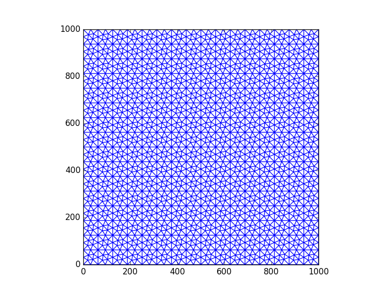
Figure 2. Mesh4

In our tests we are led to compare the initial scheme with the scheme obtained by the following modification of the diffusion–dispersion tensor, which consists in rewriting (2.3) as

$$(\mathbf{D}(x,\mathbf{u}))_{i,i}=D_{m}+|\mathbf{u}|\Big{(}(D_{l}-D_{t})\frac{\mathbf{u}_{i}^{2}}{|\mathbf{u}|^{2}}+D_{t}\Big{)},$$

setting $D_{\alpha}=\Phi d_{\alpha}$ for $\alpha=m,l,t$, and

$$(\mathbf{D}(x,\mathbf{u}))_{i,j}=|\mathbf{u}|\Big{(}(D_{l}-D_{t})\frac{\mathbf{u}_{i}\mathbf{u}_{j}}{|\mathbf{u}|^{2}}\Big{)}\hbox{ for }j\neq i.$$

Then, for some tests with too low values for $d_{m}$, $d_{l}$ or $d_{t}$, we use the centred scheme in which we replace $\mathbf{D}$ with ${\mathbf{D}}_{h}$ defined by

$$\begin{array}[]{ll}({\mathbf{D}}_{h}(x,\mathbf{u}))_{i,i}=\max\Big{(}(\mathbf{D}(x,\mathbf{u}))_{i,i},|\mathbf{u}|h\Big{)},\\ ({\mathbf{D}}_{h}(x,\mathbf{u}))_{i,j}=(\mathbf{D}(x,\mathbf{u}))_{i,j}\hbox{ for }j\neq i,\end{array}$$ (6.2)

where $h$ is the size of the mesh (note that the dimension of $D_{l}$ and $D_{t}$ is that of a length). This modification introduces some diffusion, scaled by the approximate Darcy velocity and vanishing with the mesh size. This numerical diffusion is not larger than the diffusion induced by upstream schemes, but has the added advantage of being isotropic when the numerical diffusion from upstreaming is larger in the direction of the flow. Note that the convergence analysis carried out in the previous sections also applies to $\mathbf{D}_{h}$ provided that $d_{m}$, $d_{l}$ and $d_{t}$ are all strictly positive, since for $h\leq\min(D_{l},D_{t})$ we have $\mathbf{D}_{h}=\mathbf{D}$.

6.1. Analytical solutions

Exact solutions of nonlinear models involved in groundwater flows are very rare, and often limited to 1D models or to single equations; see e.g. [52, 51]. These do not account for the coupling occurring for example in (1.1), and which is at the core of numerical issues (a poor approximation of the Darcy velocity reflects strongly on the concentration fields, which in return further degrades the Darcy velocity). In this section, we design an analytic solution for a slightly modified version of (1.1). Specifically, we remove the source and reaction terms in the concentration equation, and we consider Dirichlet boundary conditions on part of the domain. The solution however has similar features to those found in real solutions: it flows from one part of the domain to the other part, and satisfies the same strongly coupled equations inside the domain – and thus enable us to illustrate corresponding numerical challenges.

All data in this section are dimensionless. We take $\Phi=1$, $c_{0}=0$, $\mathbf{K}={\rm Id}$, $\Omega=(0,1)^{2}$, and final time $T=0.4$. Following ideas in [44], we seek a solution $(p,c)$ to (1.1) in radial coordinates $\rho$ centred at $(1,1)$. The tensor $\mathbf{D}$ is defined by (2.3) with $d_{l}=d_{t}=0$ and $d_{m}>0$ chosen such that

$$N=\frac{2}{4d_{m}}-1\in{\mathbb{N}}.$$ (6.3)

Removing the production reaction term for the equation on $c$ (see Remark 6.1 about the injection source term), this solution $(p,c)$ satisfies:

$$u_{\rho}=\frac{1}{\rho}=-\frac{1}{\mu(c(\rho,t))}\partial_{\rho}p(\rho,t),\quad(\rho,t)\in(0,\infty)\times(0,T),$$

$$\rho\partial_{t}c(\rho,t)-\partial_{\rho}\left(\rho(d_{m}\partial_{\rho}c-u_{\rho}c)\right)(\rho,t)=0,\quad(\rho,t)\in(0,\infty)\times(0,T),$$

with $c(0,t)=1$ and $c(+\infty,t)=0$. The full Darcy velocity is $\mathbf{u}(\rho,t)=u_{\rho}\mathbf{e}_{\rho}$, where $(\mathbf{e}_{\rho},\mathbf{e}_{\theta})$ are the local polar unit vectors.

Denoting by $\delta_{A}$ the Dirac measure at a point $A\in\overline{\Omega}$, we set $q^{I}(x)\,\mathrm{d}x=\frac{\pi}{2}\ \delta_{(1,1)}$. For $x=(x_{1},x_{2})\in(0,1)\times\{0\}$, $q^{P}(x)={\rm d}\theta(x_{1})$ is the lineic Dirac measure weighted by the derivate of the angle $\theta(x_{1})=OIM$ with $O=(0,0)$, $I=(1,1)$ and $M=(x_{1},0)$. For $x=(x_{1},x_{2})\in\{0\}\times(0,1)$, $q^{P}(x)={\rm d}\theta(x_{2})$ is the lineic Dirac measure weighted by the derivate of the angle $\theta(x_{2})=OIM$ with $M=(0,x_{2})$. Hence, solvent is injected at the top right corner of the domain and a mixture of oil and solvent is recovered at both sides of the domain passing by the origin, both at a rate of $\frac{\pi}{2}$. These source terms, the expression for the function $\mu$, and the values for $d_{m}$ are inspired by Tests 1 and 2 in [61, 10], in which solvent is injected at the top right corner and the mixture is produced at the bottom left corner.

Remark 6.1 (Hidden source terms).

The Darcy velocity $\mathbf{u}$ defined above satisfies $\operatorname{div}(\mathbf{u})=0$ in the sense of distributions on $\Omega$. However, one can easily check that if $\varphi\in C^{1}({\mathbb{R}}^{2})$ then, with $B_{\epsilon}$ the ball of center $(1,1)$ and radius $\epsilon$,

$$\mathrm{PV}\int_{\Omega}\mathbf{u}\cdot\nabla\varphi:=\lim_{\epsilon\to 0}\int_{\Omega\backslash B_{\epsilon}}\mathbf{u}\cdot\nabla\varphi=\langle q^{I},\varphi\rangle-\langle q^{P},\varphi\rangle,$$ (6.4)

where the duality products are understood in the sense of distributions on ${\mathbb{R}}^{2}$ (or as integrals against the measures $q^{I}$ and $q^{P}$). Here, PV denotes the ‘principal value’ of the integral, a classical notion in the context of distributions (but slightly less classical here since the singularity is on the boundary of the domain). Equation (6.4) shows that the relation $\operatorname{div}(\mathbf{u})=q^{I}-q^{P}$ is satisfied in a weak sense against test functions in $C^{1}(\overline{\Omega})$.

One could also consider that the source terms $q^{I}$ and $q^{P}$ are handled as non-homogeneous Neumann boundary conditions (which is how they are implemented in our tests). Indeed, for elliptic PDEs with Neumann boundary conditions, including measures in the boundary conditions or the same measures as ‘source terms’ of the PDE lead to the exact same weak formulations.

The same reasoning applies to the equation on $c$. Although the equation does not seem to contain any injection source term $q^{I}$, this source term is actually hidden ‘on the boundary’.

The equation on $c$ thus no longer depends on $p$, and a solution is obtained by setting $c(\rho,t)=\psi(\rho^{2}/(4d_{m}t))$, where $\psi$ satisfies

$$\forall z>0,\quad-z\psi^{\prime}(z)+N\psi^{\prime}(z)-z\psi^{\prime\prime}(z)=0,$$

with $\psi(0)=1$ and $\psi(+\infty)=0$ and $N$ defined by (6.3). This function is given by

$$\psi(z)=e^{-z}\sum_{k=0}^{N}\frac{z^{k}}{k!}.$$

We impose the nonhomogeneous Dirichlet boundary condition $c(x,t)=\psi(\rho^{2}/(4d_{m}t))$ on $[(0,1)\times\{0\}]\cup[\{0\}\times(0,1)]$, to preserve the radial symmetry of the problem and the expression of the exact solution.

Remark 6.2.

The values of $\psi$ can easily be evaluated by calculating the terms $v_{0}=0$, $v_{k+1}=\frac{z}{N-k}(v_{k}+e^{-z})$, for $k=0,\ldots,N-1$, and by setting $\psi(z)=v_{N}+e^{-z}$.

The exact solutions corresponding to these tests are shown in Figure 3. Note that in this particular situation, the values for $c$ do not depend on the function $\mu$; however, the numerical issues to approximate this solution remain since we consider the full coupled system, in which $\mu$ strongly impacts the approximation of the Darcy velocity.

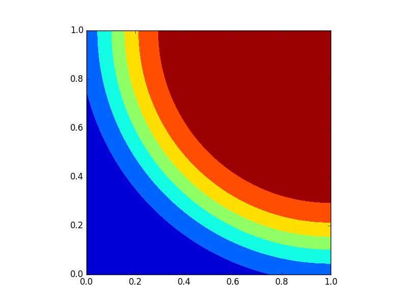
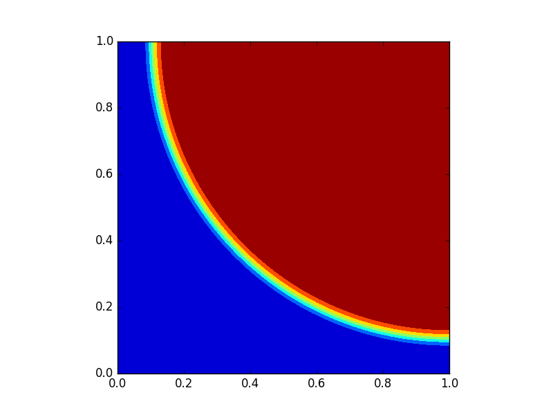
Figure 3. Exact solutions: analytical test 1 (left) corresponds to $d_{m}=0.05$; analytical test 2 (right) corresponds to $d_{m}=0.001$. Values from $0$ (dark blue) to $1$ (dark red).

6.1.1. Analytical test 1: constant viscosity, large $d_{m}$

We take here $M=1$ (hence, $\mu$ is constant) and $d_{m}=0.05$. Figure 4 presents the concentration $c$ calculated by the two schemes; $L^{1}$ and $L^{2}$ errors for various meshes and time steps are shown in Table 1. All these results indicate a clear convergence of both schemes, with a rate close to $\mathcal{O}(h^{2}+\delta t)$, as expected for the first order Schemes A and B with implicit time stepping.

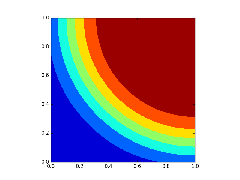
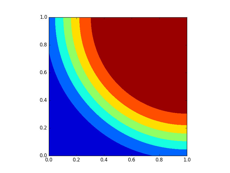
Figure 4. Analytical test 1, concentration with centred scheme: Scheme A on a $50\times 50$ mesh with time step $0.01$ (left); Scheme B on Mesh5 with time step $0.005$ (right). Values from $0$ (dark blue) to $1$ (dark red).

Scheme	Mesh	$\delta t$	$L^{1}$ error	$L^{2}$ error
A	$25\times 25$	$0.02$	2.38E-2	3.23E-2
	$50\times 50$	$0.005$	6.69E-3	9.10E-3
	$100\times 100$	$0.00125$	1.73E-3	2.36E-3
B	mesh4	$0.02$	2.39E-2	3.20E-2
	mesh5	$0.005$	6.70E-3	9.04E-3
	mesh6	$0.00125$	1.73E-3	2.38E-3

Table 1. Analytical test 1: $L^{1}$ and $L^{2}$ errors at the final time $T=0.4$.

6.1.2. Analytical test 2: varying viscosity, small $d_{m}$

In this test, we let $M=40$ and $d_{m}=0.001$. The viscosity therefore varies, the natural diffusion is very small, and the problem is highly advection-dominated. As can be seen in Figures 5–6 and in Tables 2–3, the centred versions of Schemes A and B produce unacceptable solutions, and do not seem to converge. The same conclusion holds for upstream versions of these schemes: even though the grid effects seem to be somehow mitigated by the upstreaming, the solutions are still very distorted and there is no apparent numerical convergence.

The reasons for this failure of both the centred and upstream schemes might be found in the combination of two factors: the viscosity varying with $c$ negatively impacts the quality of the numerical Darcy velocity, which in turns generate bad fluxes when used in the concentration equation; in case of upstreaming, the numerical diffusion introduced by this process is anisotropic. It occurs mostly in the direction of the numerical Darcy velocity, and a poorly approximated velocity therefore results in numerical diffusion in unphysical directions – typically, directions dictated by the grid rather than the genuine flow.

To mitigate these issues, we use the modification (6.2). The results presented in Figures 5–6 and in Tables 2–3 show a clear improvement of the numerical solution. It has the expected shape, and convergence seems to occur (even though at a slow rate).

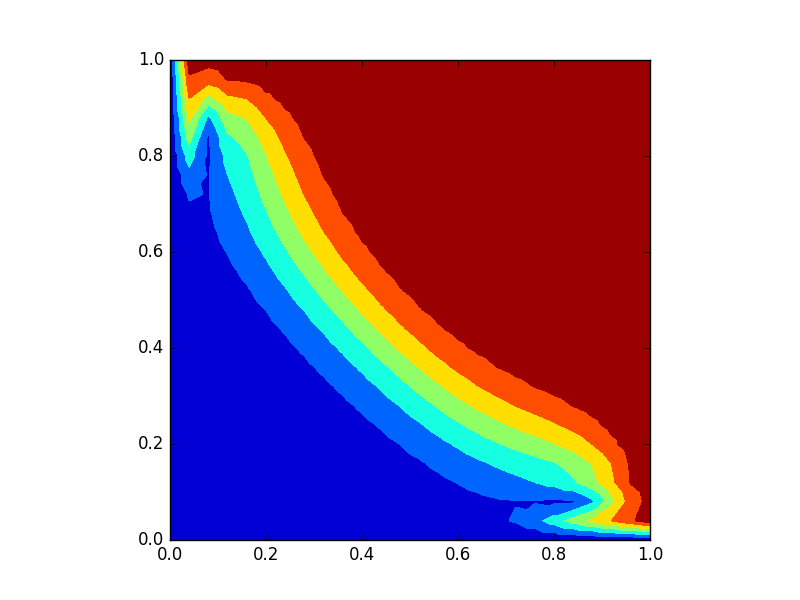
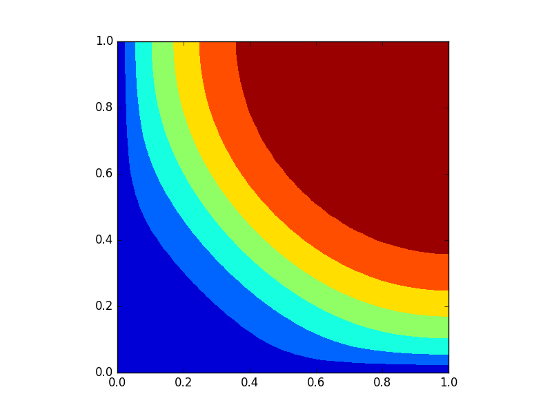
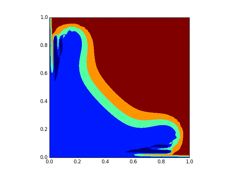
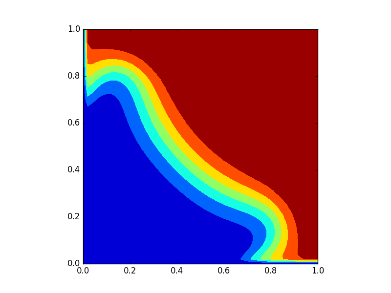
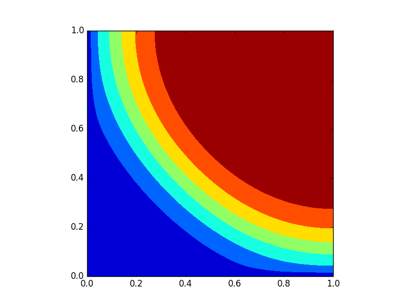
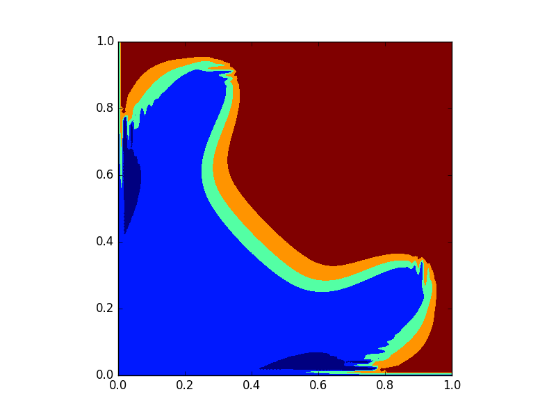
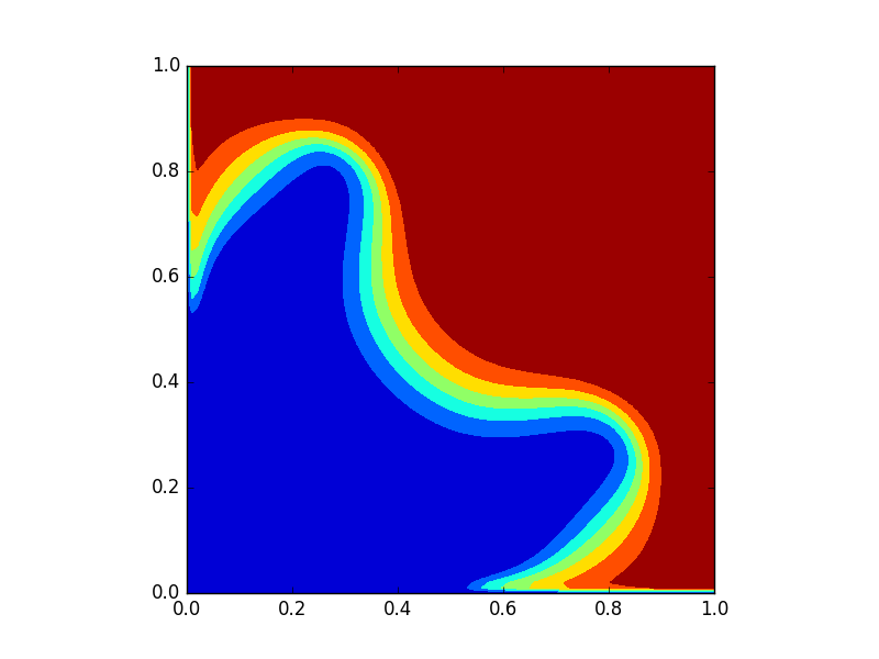
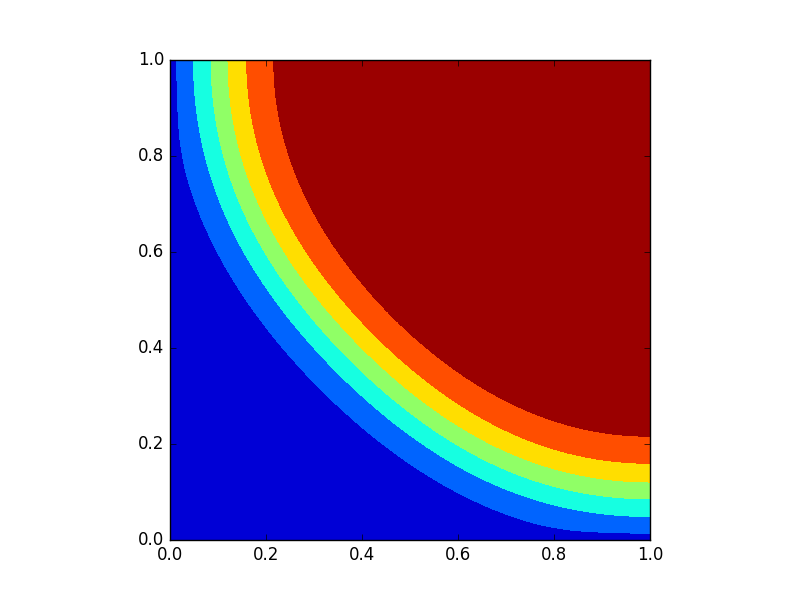
Figure 5. Analytical test 2, Scheme A. From top to bottom: $25\times 25$ mesh and time step $0.02$; $50\times 50$ mesh and time step $0.01$; $100\times 100$ mesh and time step $0.005$. From left to right: centred, upstream, modification by (6.2) (right). Values from $0$ (dark blue) to $1$ (dark red).

Variant	Mesh	$\delta t$	$L^{1}$ error	$L^{2}$ error
centred	$25\times 25$	0.02	1.06E-1	2.00E-1
	$50\times 50$	0.01	1.32E-1	2.77E-1
	$100\times 100$	0.005	1.71E-1	3.49E-1
upstream	$25\times 25$	0.02	1.51E-1	2.04E-1
	$50\times 50$	0.01	1.35E-1	2.65E-1
	$100\times 100$	0.005	2.00E-1	3.78E-1
With (6.2)	$25\times 25$	0.02	1.51E-1	2.04E-1
	$50\times 50$	0.01	1.11E-1	1.66E-1
	$100\times 100$	0.005	7.80E-2	1.32E-1

Table 2. Analytical test 2, errors with three variants of Scheme A: centred, upstream and with (6.2)

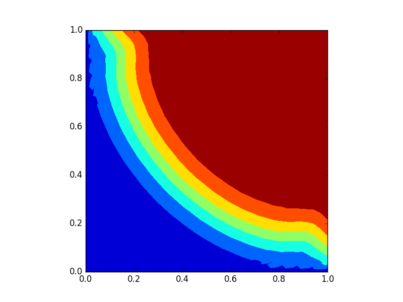
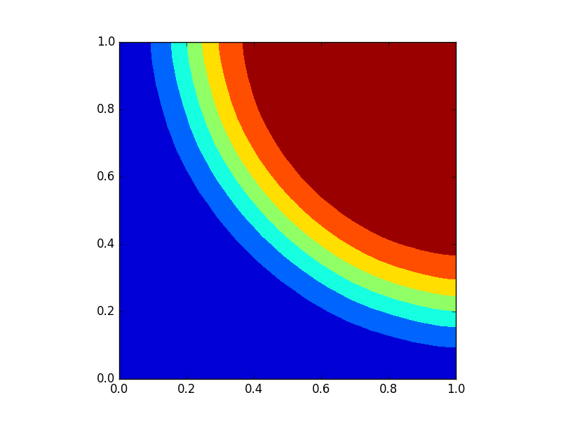
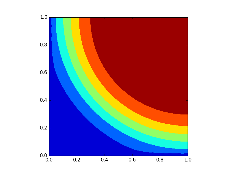
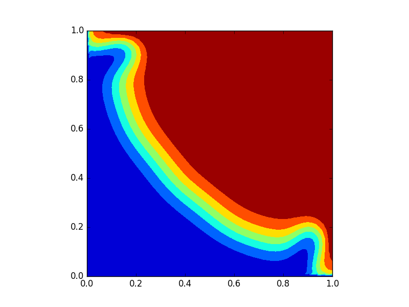
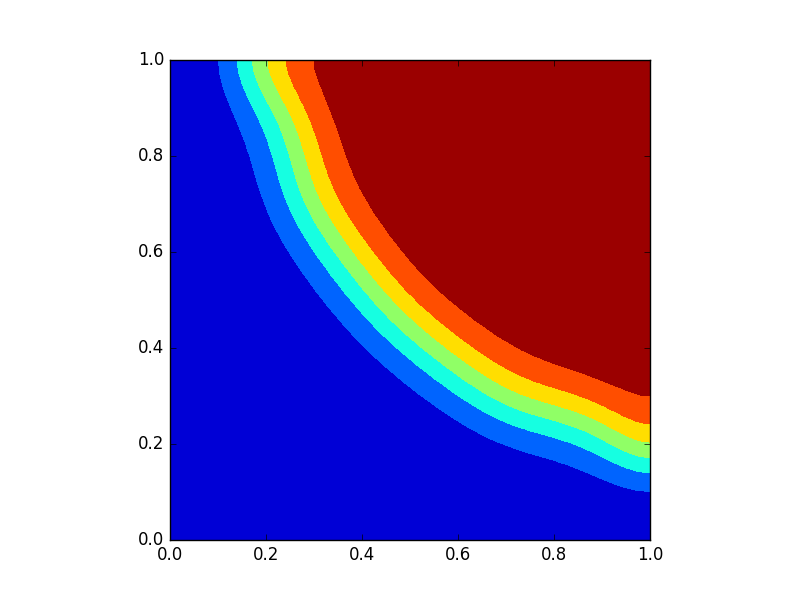
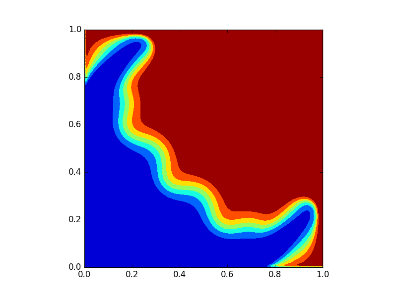
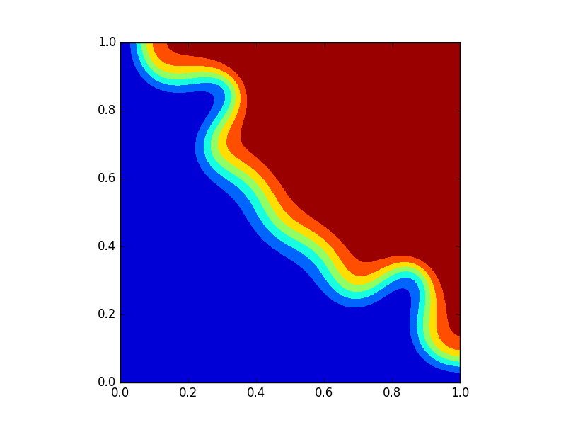
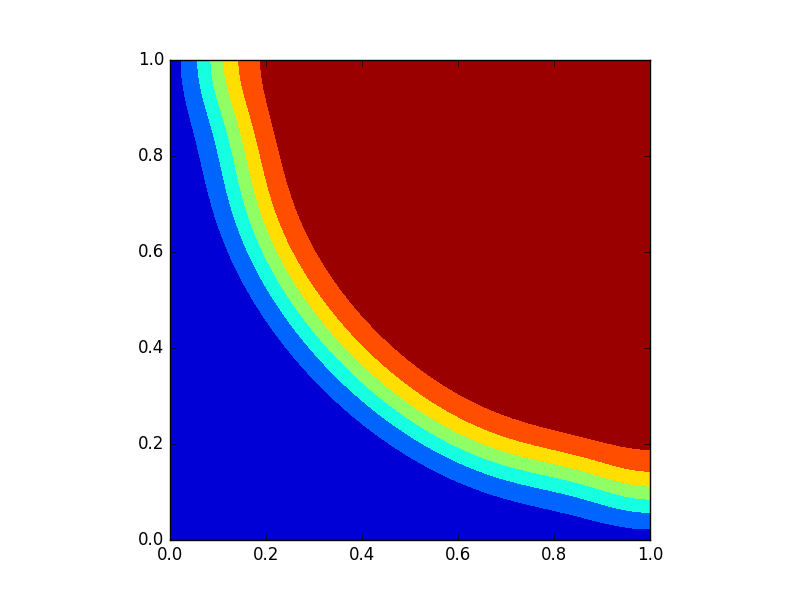
Figure 6. Analytical test 2, Scheme B. From top to bottom: Mesh4 and time step $0.02$; Mesh5 and time step $0.01$; Mesh6 and time step $0.005$. From left to right: centred, upstream, modification by (6.2) (right). Values from $0$ (dark blue) to $1$ (dark red).

Variant	Mesh	$\delta t$	$L^{1}$ error	$L^{2}$ error
centred	Mesh4	0.02	9.05E-2	1.46E-1
	Mesh5	0.01	7.23E-2	1.47E-1
	Mesh6	0.005	9.42E-2	2.29E-1
upstream	Mesh4	0.02	1.71E-1	2.98E-1
	Mesh5	0.01	1.58E-1	3.03E-1
	Mesh6	0.005	1.66E-1	3.34E-1
With (6.2)	Mesh4	0.02	1.22E-1	1.77E-1
	Mesh5	0.01	8.55E-2	1.39E-1
	Mesh6	0.005	5.65E-2	1.04E-1

Table 3. Analytical test 2, errors with three variants of Scheme B: centred, upstream and with (6.2)

6.2. Comparison with test cases from the literature

We now apply Schemes A and B defined in Section 3.2 to the first and second test cases in Wang-et-al. [61] and Chainais-Hillairet–Droniou [10]. In these test cases, the source terms do not satisfy Hypotheses (2.2g), but, as we show below and as already noted in [10], this does not seem to prevent numerical convergence. Additionally, in the second test case, the diffusion–dispersion tensor $\mathbf{D}$ does not satisfy all the hypotheses in (2.2c) (it is only positive, not uniformly positive-definite). This will force us, as in the analytical test 2, to introduce some additional vanishing diffusion (see Section 6.2.2).

In both cases the domain is a two-dimensional reservoir $\Omega=(0,1000)^{2}$ ft² and the final time is set $T=1080$ days ($\approx$ 3 years). Denoting by $\delta_{A}$ the Dirac measure at a point $A\in\overline{\Omega}$, set $\hat{c}(x)=1$, $q^{I}(x)\,\mathrm{d}x=30\ \delta_{(1000,1000)}$ and $q^{P}(x)\,\mathrm{d}x=30\ \delta_{(0,0)}$; hence, solvent is injected at the top right corner of the domain and a mixture of oil and solvent is recovered at the bottom left corner, both at a rate of $30$ ft²/day. Set $\Phi(x)=0.1$, $c_{0}(x)=0$ and, for almost-every $x\in\Omega$, $\mathbf{K}(x)=k\mathbf{I}$ with $k=80$ md.

Remark 6.3 (Implementation of the Dirac measures).

For both schemes, the reconstructions $\Pi_{\mathcal{D}}$ provide piecewise constant functions on a certain mesh. In the case of Scheme A, the boundary cells of this mesh are cut in 2 at the boundary edges and in four at the corners, so that the centers of the cells are located on the boundary. In the case of Scheme B, these cells are dual cells centred on the vertices of the triangular mesh. In both cases, there are four cells whose centre is precisely located at a corner of $\Omega$. In our test cases, the Dirac masses $q^{+}$ and $q^{-}$ in (3.3a)–(3.3b) are simply taken into account in the source terms corresponding to the two corner cells where they are located.

6.2.1. Test 1: constant viscosity, only molecular diffusion

We consider Test 1 of [61]. Thus, $M=1$ and the diffusion–dispersion tensor is defined by (2.3) with $\Phi d_{m}=1$ ft²/day, $\Phi d_{l}=0$ ft and $\Phi d_{t}=0$ ft. $\mathbf{D}$ then satisfies the coercivity properties that ensures that the reconstructed gradient of the concentration remains bounded. We observe a clear numerical convergence, comparing the refinement in space and time of both Schemes A and B (see Figure 7).

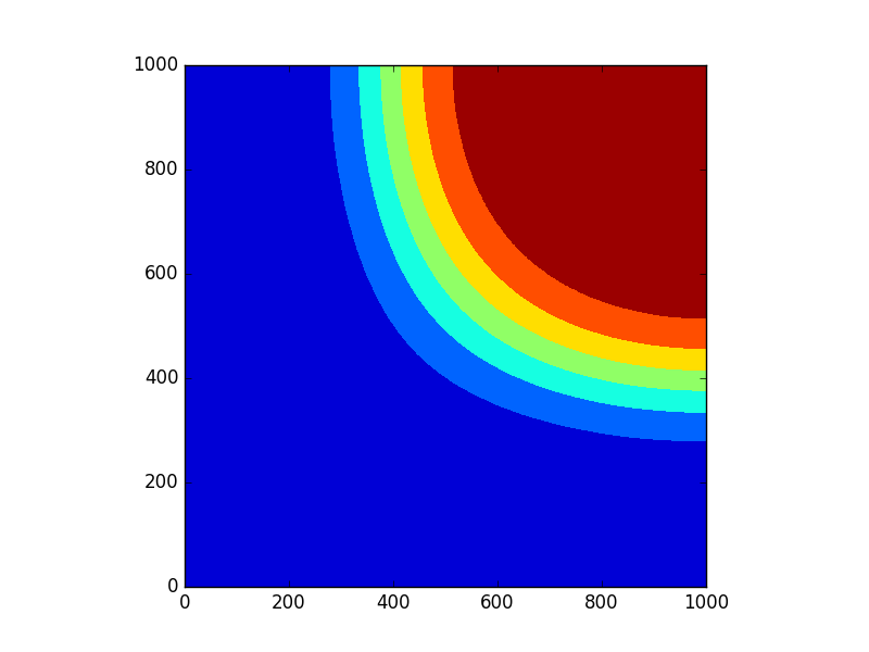
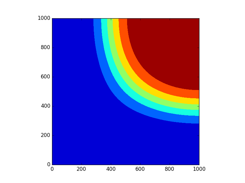
Figure 7. Test 1, concentration with centred scheme. Top: Scheme A : $50\times 50$ mesh with time step $18$ days (left); $100\times 100$ mesh with time step $9$ days (right). Bottom: Scheme B on Mesh4 with time step $18$ days (left); on Mesh5 with time step $9$ days (right). Values from $0$ (dark blue) to $1$ (dark red).

6.2.2. Test 2: transverse and longitudinal dispersion, no molecular diffusion

We now consider Test 2 of [61], in which $M=41$, $\Phi d_{m}=0$ ft²/day, $\Phi d_{l}=5$ ft and $\Phi d_{t}=0.5$ ft. Let us first examine the results provided by Schemes A and B used without modification.

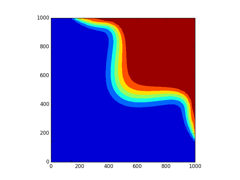
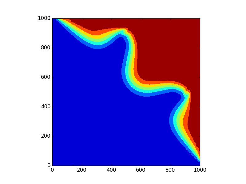
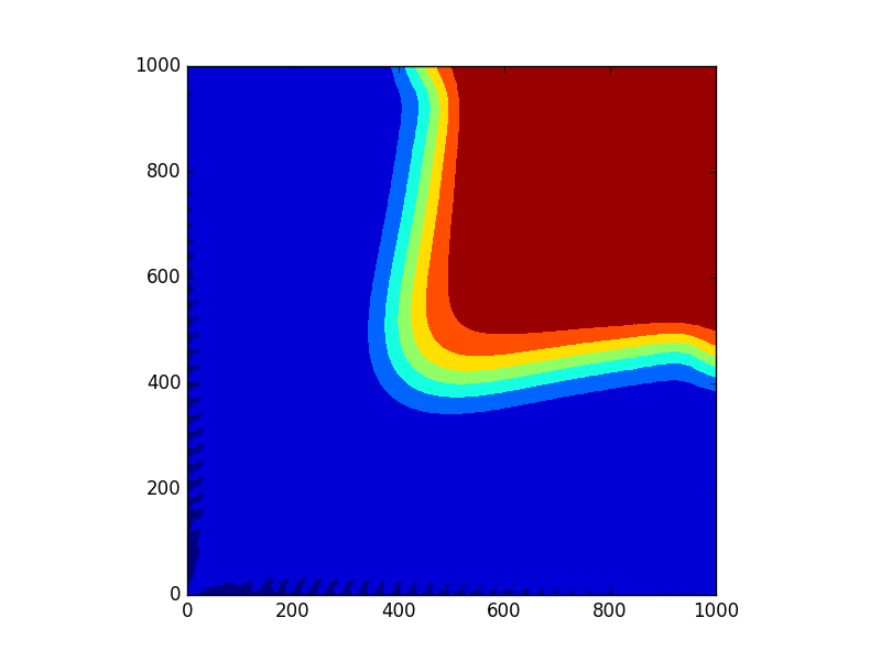
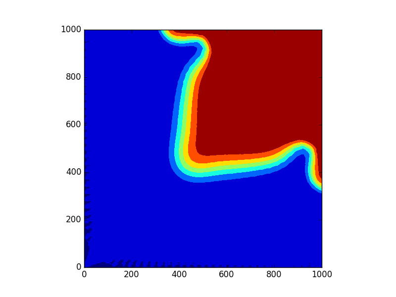
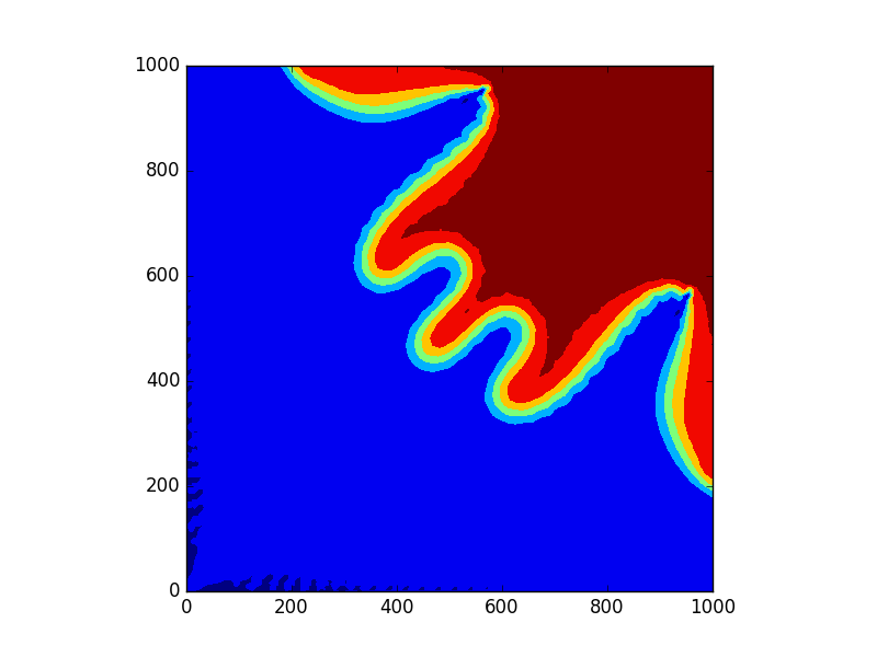
Figure 8. Top: Concentration with scheme A, $50\times 50$ mesh with time step $36$ days (left), $18$ days (middle), $9$ days (right). Bottom: same with scheme B on Mesh5. Values from $0$ (dark blue) to $1$ (dark red).

Figure 8 shows the contours of the approximate concentration obtained at the final time $T$. We notice that many published results consider time steps equal to or larger than 36 days; with such a time step, the result obtained with scheme B is comparable to the ones in the literature. We notice however that, for smaller time steps, the results are no longer so nice. In that case, the transversal diffusion is not sufficient to stabilize the scheme, and introducing a vanishing diffusion becomes necessary.

Remark 6.4.

The reason for the better results observed with a larger time step can perhaps be found in the term $\frac{1}{2}\left(\Pi_{\mathcal{D}}c^{(n+1)}-\Pi_{\mathcal{D}}c^{(n)}\right)^{2}$ in (4.5). This term can be seen as an approximation of $\delta t\int_{0}^{T}\int_{\Omega}(\partial_{t}c)^{2}$. When carried over in (4.6), it therefore contributes to controling this time derivative of the concentration, which can result in an improved stability of the scheme. For smaller time steps, this control becomes less efficient due to the $\delta t$ factor.

We saw in the analytical test 2 that upstreaming the schemes was not necessarily a good option to recover a stable and accurate solution. This is confirmed here in Figure 9: upstreaming is not a good paliative for the lack of diffusion (especially for Scheme A).

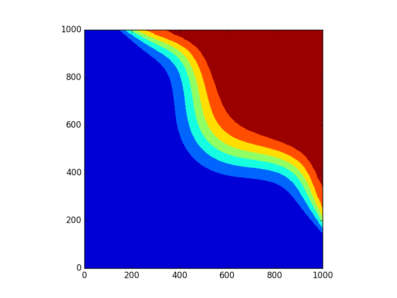
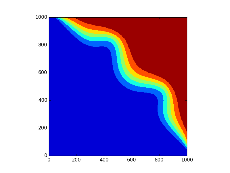
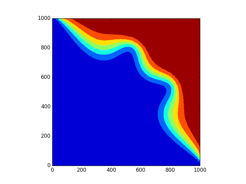
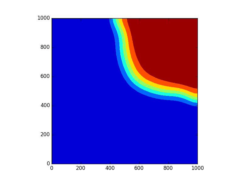
Figure 9. Top: Concentration with upstream version of scheme A, $50\times 50$ mesh with time step $36$ days (left), $18$ days (middle), $9$ days (right). Bottom: same with upstream version of scheme B on Mesh5. Values from $0$ (dark blue) to $1$ (dark red).

To recover a stable and accurate solution, we use the modification (6.2). The results obtained with this modified scheme are shown in Figure 10. As can be seen, both Schemes A and B then display a nice numerical convergence to the expected solution, as the time step decreases.

It was proved in [33] that, when the molecular diffusion vanishes, weak solutions to (1.1) converge to solutions of the same model with zero molecular diffusion; the arguments given in [33] are applicable to ${\mathbf{D}}_{h}$ defined by (6.2) and show that, as $h\to 0$, the solution with this modified diffusion–dispersion tensor converges to a solution of the model with zero molecular diffusion. This justifies using (6.2) in numerical approximations.

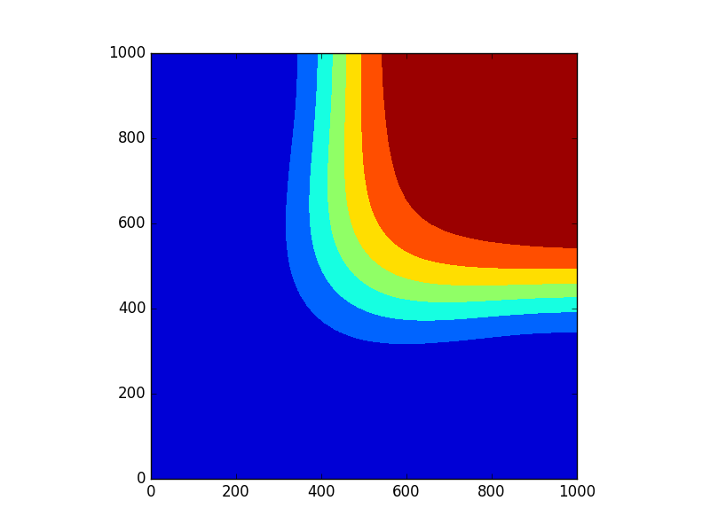
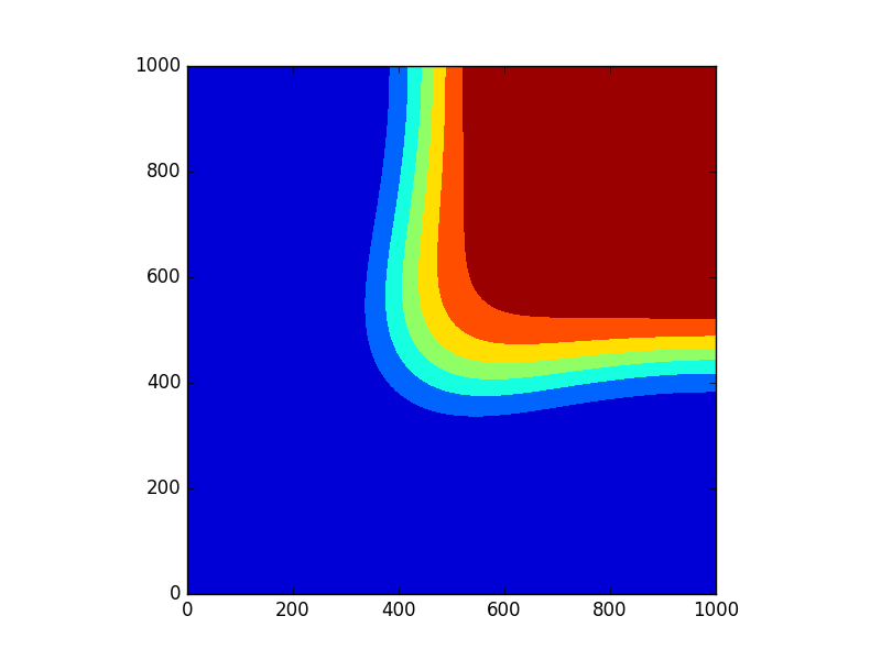
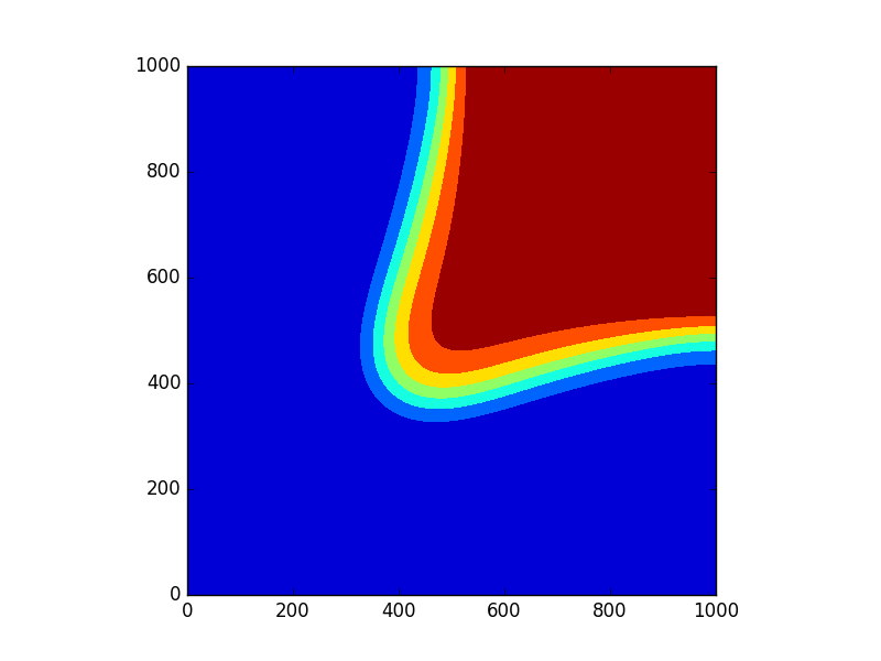
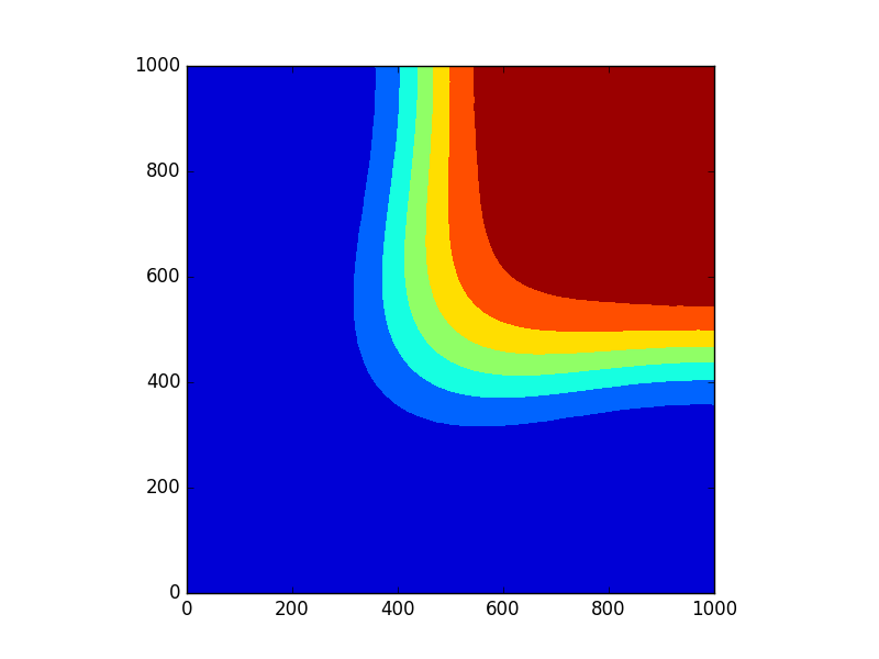
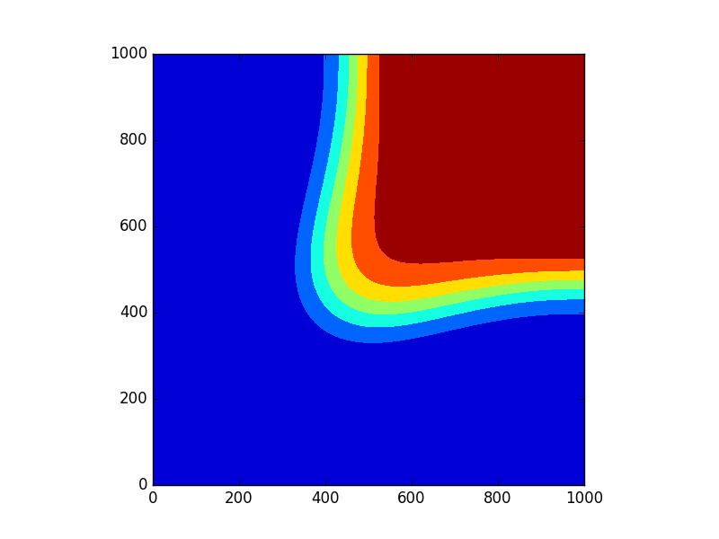
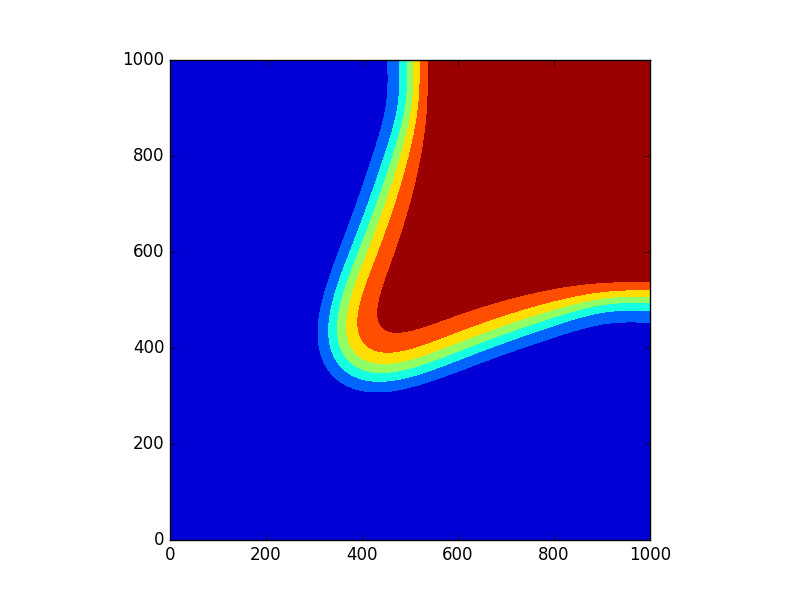
Figure 10. Top: Concentration using (6.2) with Scheme A: $50\times 50$ mesh with time step $36$ days (left), $100\times 100$ mesh with time step $18$ days (middle), $200\times 200$ mesh with time step $9$ days (right). Bottom: same with Scheme B, Mesh4 with time step $36$ days (left), Mesh5 with time step $18$ days (middle), Mesh6 with time step $9$ days (right). Values from $0$ (dark blue) to $1$ (dark red).

7. Conclusion

We applied the gradient discretisation method to a model of miscible incompressible flows in porous media. The GDM framework enables us to write in a unified format many different numerical methods for this model, from finite differences, to finite volumes and finite elements. We considered a centred discretisation of the advective terms in the concentration equation. The convergence analysis was performed using compactness techniques, to avoid imposing non-physical regularity assumptions on the data or the solution to the model. It applies to all methods fitting into the GDM framework. A novelty of our analysis compared to similar results in the literature is a uniform-in-time, $L^{2}(\Omega)$-strong convergence result for the approximate concentration.

We showed numerical results using two schemes that fit into the GDM framework: a finite-difference scheme written on Cartesian meshes, and a mass-lumped $P^{1}$ finite element scheme on triangles. It was demonstrated, on both analytical and physical test cases, that centred and upstream schemes behave badly in the case of varying viscosity and small physical diffusion. A modification was then proposed and shown to lead to stable and accurate solutions. This modification consists introducing some vanishing numerical diffusion, designed to be isotropic, to scale as the magnitude of the Darcy velocity, and to vanish with the mesh size in the same was as upstream numerical diffusions.

Appendix A Convergence lemmas

For proofs of the first three of these lemmas, see [32]. Lemma A.4 is proved in [26], and the interpolation lemma A.5 is a special case of [28, Lemma 4.10].

Lemma A.1.

Let $\Omega$ be a bounded subset of ${\mathbb{R}}^{N}$, $N\in{\mathbb{N}}$ and for each $n\in{\mathbb{N}}$, let $H_{n}:\Omega\times{\mathbb{R}}^{N}\to{\mathbb{R}}$ be a Carathéodory function such that

• there exist positive constants $C$ and $\gamma$ such that for almost-every $x\in\Omega$,

  $$|H_{n}(x,\xi)|\leq C(1+|\xi|^{\gamma}),\quad\mbox{$\forall\xi\in{\mathbb{R}}^{N}$, $\forall n\in{\mathbb{N}}$,}$$ (A.1)

• there is a Carathéodory function $H:\Omega\times{\mathbb{R}}^{N}\to{\mathbb{R}}$ such that for a.e. $x\in\Omega$,

  $$H_{n}(x,\cdot)\to H(x,\cdot)\quad\mbox{uniformly on compact sets as $n\to\infty$.}$$ (A.2)

If $p\in[\max(1,\gamma),\infty)$ and $(u_{n})_{n\in{\mathbb{N}}}\subset L^{p}(\Omega)^{N}$ is a sequence with $u_{n}\to u$ in $L^{p}(\Omega)^{N}$ as $n\to\infty$, then $H_{n}(\cdot,u_{n})\to H(\cdot,u)$ in $L^{p/\gamma}(\Omega)$ as $n\to\infty$.

Corollary A.2.

Let $\Omega$, $H_{n}$ and $H$ satisfy the hypotheses of Lemma A.1. If $p,q\in[\max(1,\gamma),\infty)$ and $(u_{n})_{n\in{\mathbb{N}}}\subset L^{p}(0,T;L^{q}(\Omega)^{N})$ is a sequence with $u_{n}\to u$ in $L^{p}(0,T;L^{q}(\Omega)^{N})$ as $n\to\infty$, then $H_{n}(\cdot,u_{n})\to H(\cdot,u)$ in $L^{p/\gamma}(0,T;L^{q/\gamma}(\Omega))$ as $n\to\infty$.

Lemma A.3.

Let $\Omega$ be a bounded, open subset of ${\mathbb{R}}^{N}$ and for every $n\in{\mathbb{N}}$, let $w_{n}:\Omega\times(0,T)\to{\mathbb{R}}$ and $v_{n}:\Omega\times(0,T)\to{\mathbb{R}}$ be such that $w_{n}\to w$ in $L^{r_{1}}(0,T;L^{s_{1}}(\Omega))$, and $v_{n}\rightharpoonup v$ weakly in $L^{r_{2}}(0,T;L^{s_{2}}(\Omega))$, where $r_{1},r_{2},s_{1},s_{2}\geq 1$ are such that $1/r_{1}+1/r_{2}\leq 1$ and $1/s_{1}+1/s_{2}\leq 1$. Suppose also that the sequence $(w_{n}v_{n})_{n\in{\mathbb{N}}}$ is bounded in $L^{a}(0,T;L^{b}(\Omega))$, where $a,b\in(1,\infty)$. Then $w_{n}v_{n}\rightharpoonup wv$ weakly in $L^{a}(0,T;L^{b}(\Omega))$.

Lemma A.4.

Let $(K,d_{K})$ be a compact metric space, $(E,d_{E})$ a metric space. Denote by $\mathcal{F}(K,E)$ the space of functions $K\to E$, endowed with the uniform metric $d_{\mathcal{F}}(v,w)=\sup_{s\in K}d_{E}(v(s),w(s))$ (note that this metric may take infinite values).

Let $(v_{n})_{n\in{\mathbb{N}}}$ be a sequence in $\mathcal{F}(K,E)$ and $v:K\to E$ be continuous. Then $v_{n}\to v$ for $d_{\mathcal{F}}$ if and only if, for any $s\in K$ and any sequence $(s_{n})_{n\in{\mathbb{N}}}\subset K$ converging to $s$ for $d_{K}$, $v_{n}(s_{n})\to v(s)$ for $d_{E}$.

Lemma A.5 (GDM interpolation of space-time functions).

Let $(\mathcal{D}_{m})_{m\in{\mathbb{N}}}$ be a consistent sequence of gradient discretisations in the sense of Definition 3.4. Let $\theta\in\{0,1\}$ and, if $v\in X_{\mathcal{D}_{m}}$, set, for all $n=0,\ldots,N_{m}-1$ and $t\in(t^{(n)},t^{(n+1)}]$

$$\Pi_{\mathcal{D}_{m}}^{(\theta)}v(t)=\Pi_{\mathcal{D}_{m}}v^{(n+\theta)}\quad\mbox{ and }\quad\nabla_{\mathcal{D}_{m}}^{(\theta)}(t)=\nabla_{\mathcal{D}_{m}}v^{(n+\theta)}$$

(hence, using the notations (3.1), $\Pi_{\mathcal{D}_{m}}^{(1)}=\Pi_{\mathcal{D}_{m}}$ and $\Pi_{\mathcal{D}_{m}}^{(0)}=\Pi_{\mathcal{D}_{m}}^{\mathrm{ex}}$). Let $\varphi\in L^{2}(0,T;H^{1}(\Omega))$. Then there exists $v_{m}=(v_{m}^{(n)})_{n=0,\ldots,N_{m}}\in X_{\mathcal{D}_{m}}^{N_{m}+1}$ such that, as $m\to\infty$,

$$\Pi_{\mathcal{D}_{m}}^{(\theta)}v_{m}\to\varphi\mbox{ in $L^{2}(0,T;L^{2}(\Omega))$}\quad\mbox{ and }\quad\nabla_{\mathcal{D}_{m}}^{(\theta)}v_{m}\to\nabla\varphi\mbox{ in $L^{2}(0,T;L^{2}(\Omega)^{d})$.}$$

If, moreover, $\partial_{t}\varphi\in L^{2}(0,T;L^{2}(\Omega))$ then $(v_{m})_{m\in{\mathbb{N}}}$ can be chosen such that, additionally,

$$\delta_{\mathcal{D}_{m}}v_{m}\to\partial_{t}\varphi\mbox{ in $L^{2}(0,T;L^{2}(\Omega))$}\quad\mbox{ and }\quad\Pi_{\mathcal{D}_{m}}v_{m}^{(0)}\to\varphi(\cdot,0)\mbox{ in $L^{2}(\Omega)$}.$$

References

- [1] I. Aavatsmark, T. Barkve, O. Boe, and T. Mannseth. Discretization on non-orthogonal, quadrilateral grids for inhomogeneous, anisotropic media. J. Comput. Phys., 127(1):2–14, 1996.
- [2] B. Amaziane and M. El Ossmani. Convergence analysis of an approximation to miscible fluid flows in porous media by combining mixed finite element and finite volume methods. Numer. Methods Partial Differential Equations, 24(3):799–832, 2008.
- [3] B. Andreianov, F. Boyer, and F. Hubert. Discrete duality finite volume schemes for Leray-Lions-type elliptic problems on general 2D meshes. Numer. Methods Partial Differential Equations, 23(1):145–195, 2007.
- [4] S. Bartels, M. Jensen, and R. Müller. Discontinuous Galerkin finite element convergence for incompressible miscible displacement problems of low regularity. SIAM J. Numer. Anal., 47(5):3720–3743, 2009.
- [5] L. Beirão da Veiga, J. Droniou, and G. Manzini. A unified approach for handling convection terms in finite volumes and mimetic discretization methods for elliptic problems. IMA J. Numer. Anal., 31(4):1357–1401, 2011.
- [6] F. Brezzi, A. Buffa, and K. Lipnikov. Mimetic finite differences for elliptic problems. M2AN Math. Model. Numer. Anal., 43(2):277–295, 2009.
- [7] F. Brezzi and M. Fortin. Mixed and hybrid finite element methods, volume 15 of Springer Series in Computational Mathematics. Springer-Verlag, New York, 1991.
- [8] F. Brezzi, K. Lipnikov, and V. Simoncini. A family of mimetic finite difference methods on polygonal and polyhedral meshes. Math. Models Methods Appl. Sci., 15(10):1533–1551, 2005.
- [9] M.A. Celia, T.F. Russell, I. Herrera, and R.E. Ewing. An Eulerian-Lagrangian localized adjoint method for the advection-diffusion equation. Advances in Water Resources, 13(4):187–206, 1990.
- [10] C. Chainais-Hillairet and J. Droniou. Convergence analysis of a mixed finite volume scheme for an elliptic-parabolic system modeling miscible fluid flows in porous media. SIAM J. Numer. Anal., 45(5):2228–2258, 2007.
- [11] C. Chainais-Hillairet, S. Krell, and A. Mouton. Study of discrete duality finite volume schemes for the Peaceman model. SIAM J. Sci. Comput., 35(6):A2928–A2952, 2013.
- [12] C. Chainais-Hillairet, S. Krell, and A. Mouton. Convergence analysis of a DDFV scheme for a system describing miscible fluid flows in porous media. Numer. Methods Partial Differential Equations, 31(3):723–760, 2015.
- [13] G. Chavent and J. Jaffré. Mathematical Models and Finite Elements for Reservoir Simulation. Studies in Mathematics and its Applications, Vol. 17. North-Holland, Amsterdam, 1986.
- [14] Z. Chen and R. Ewing. Mathematical analysis for reservoir models. SIAM J. Math. Anal., 30(2):431–453, 1999.
- [15] P. G. Ciarlet and J.-L. Lions, editors. Handbook of numerical analysis. Vol. II. Handbook of Numerical Analysis, II. North-Holland, Amsterdam, 1991. Finite element methods. Part 1.
- [16] Y. Coudière and F. Hubert. A 3D discrete duality finite volume method for nonlinear elliptic equations. SIAM J. Sci. Comput., 33(4):1739–1764, 2011.
- [17] M. Crouzeix and P.-A. Raviart. Conforming and nonconforming finite element methods for solving the stationary Stokes equations. I. Rev. Française Automat. Informat. Recherche Opérationnelle Sér. Rouge, 7(R-3):33–75, 1973.
- [18] B.L. Darlow, R.E. Ewing, and M.F. Wheeler. Mixed finite element method for miscible displacement problems in porous media. Soc. Pet. Eng. J., 24(04):391–398, 1984.
- [19] D. Antonio Di Pietro and A. Ern. Mathematical aspects of discontinuous Galerkin methods, volume 69 of Mathématiques & Applications (Berlin) [Mathematics & Applications]. Springer, Heidelberg, 2012.
- [20] J. Douglas, R.E. Ewing, and M.F. Wheeler. The approximation of the pressure by a mixed method in the simulation of miscible displacement. RAIRO Anal. Numér., 17(1):17–33, 1983.
- [21] J. Douglas, Jr. The numerical solution of a compositional model in petroleum reservoir engineering. In Numerical Solution of Field Problems in Continuum Physics (Proc. Sympos. Appl. Math., Durham, N.C., 1968), SIAM-AMS Proc., Vol. II, pages 54–59. Amer. Math. Soc., Providence, R.I., 1970.
- [22] J. Douglas, Jr. Finite difference methods for two-phase incompressible flow in porous media. SIAM J. Numer. Anal., 20(4):681–696, 1983.
- [23] J. Droniou. Intégration et espaces de sobolev à valeurs vectorielles. Polycopiés de l’Ecole Doctorale de Mathématiques-Informatique de Marseille, available at hal.archives-ouvertes.fr/hal-01382368, 2001.
- [24] J. Droniou. Finite volume schemes for diffusion equations: introduction to and review of modern methods. Math. Models Methods Appl. Sci., 24(8):1575–1619, 2014.
- [25] J. Droniou and R. Eymard. A mixed finite volume scheme for anisotropic diffusion problems on any grid. Numer. Math., 105(1):35–71, 2006.
- [26] J. Droniou and R. Eymard. Uniform-in-time convergence of numerical methods for non-linear degenerate parabolic equations. Numer. Math., 132(4):721–766, 2016.
- [27] J. Droniou, R. Eymard, and P. Feron. Gradient Schemes for Stokes problem. IMA J. Numer. Anal., 36(4):1636–1669, 2016.
- [28] J. Droniou, R. Eymard, T. Gallouët, C. Guichard, and R. Herbin. The gradient discretisation method. Mathematics & Applications. Springer, Heidelberg, 2018. To appear. https://hal.archives-ouvertes.fr/hal-01382358.
- [29] J. Droniou, R. Eymard, T. Gallouët, and R. Herbin. A unified approach to mimetic finite difference, hybrid finite volume and mixed finite volume methods. Math. Models Methods Appl. Sci., 20(2):265–295, 2010.
- [30] J. Droniou, R. Eymard, T. Gallouët, and R. Herbin. Gradient schemes: a generic framework for the discretisation of linear, nonlinear and nonlocal elliptic and parabolic equations. Math. Models Methods Appl. Sci. (M3AS), 23(13):2395–2432, 2013.
- [31] J. Droniou, R. Eymard, and R. Herbin. Gradient schemes: generic tools for the numerical analysis of diffusion equations. ESAIM Math. Model. Numer. Anal., 50(3):749–781, 2016.
- [32] J. Droniou and K.S. Talbot. On a miscible displacement model in porous media flow with measure data. SIAM J. Math. Anal., 46(5):3158–3175, 2014.
- [33] Jérôme Droniou and Kyle S. Talbot. Analysis of miscible displacement through porous media with vanishing molecular diffusion and singular wells. 2018.
- [34] M.G. Edwards and C.F. Rogers. Finite volume discretization with imposed flux continuity for the general tensor pressure equation. Comput. Geosci., 2(4):259–290, 1998.
- [35] A. Ern and J.-L. Guermond. Theory and practice of finite elements, volume 159 of Applied Mathematical Sciences. Springer-Verlag, New York, 2004.
- [36] R.E. Ewing. Problems arising in the modeling of processes for hydrocarbon recovery. In R.E. Ewing, editor, The Mathematics of Reservoir Simulation, Frontiers in Applied Mathematics, pages 3–34. SIAM, Philadelphia, 1983.
- [37] R.E. Ewing, T.F. Russell, and M.F. Wheeler. Convergence analysis of an approximation of miscible displacement in porous media by mixed finite elements and a modified method of characteristics. Comput. Methods Appl. Mech. Engrg., 47(1-2):73–92, 1984.
- [38] R.E. Ewing and M.F. Wheeler. Galerkin methods for miscible displacement problems in porous media. SIAM J. Numer. Anal., 17(3):351–365, 1980.
- [39] R.E. Ewing and M.F. Wheeler. Galerkin methods for miscible displacement problems with point sources and sinks—unit mobility ratio case. In Mathematical methods in energy research (Laramie, Wyo., 1982/1983), pages 40–58. SIAM, Philadelphia, PA, 1984.
- [40] R. Eymard, P. Feron, and C. Guichard. Family of convergent numerical schemes for the incompressible Navier–Stokes equations. Mathematics and Computers in Simulation, 144(C):196–218, 2018.
- [41] R. Eymard, T. Gallouët, C. Guichard, R. Herbin, and R. Masson. TP or not TP, that is the question. Comput. Geosci., 18(3-4):285–296, 2014.
- [42] R. Eymard, T. Gallouët, and R. Herbin. Discretization of heterogeneous and anisotropic diffusion problems on general nonconforming meshes SUSHI: a scheme using stabilization and hybrid interfaces. IMA J. Numer. Anal., 30(4):1009–1043, 2010.
- [43] R. Eymard, C. Guichard, and R. Herbin. Small-stencil 3D schemes for diffusive flows in porous media. ESAIM Math. Model. Numer. Anal., 46(2):265–290, 2012.
- [44] R. Eymard, C. Guichard, and R. Masson. Grid orientation effect in coupled finite volume schemes. IMA J. Numer. Anal., 33(2):582–608, 2013.
- [45] P. Fabrie and T. Gallouët. Modelling wells in porous media flow. Math. Models Methods Appl. Sci., 10(5):673–709, 2000.
- [46] X. Feng. On existence and uniqueness results for a coupled system modeling miscible displacement in porous media. J. Math. Anal. Appl., 194(3):883–910, 1995.
- [47] X. Feng. Recent developments on modeling and analysis of flow of miscible fluids in porous media. In Fluid flow and transport in porous media: mathematical and numerical treatment (South Hadley, MA, 2001), volume 295 of Contemp. Math., pages 229–240. Amer. Math. Soc., Providence, RI, 2002.
- [48] Raphaèle Herbin and Florence Hubert. Benchmark on discretization schemes for anisotropic diffusion problems on general grids. In Finite volumes for complex applications V, pages 659–692. ISTE, London, 2008.
- [49] F. Hermeline. Approximation of diffusion operators with discontinuous tensor coefficients on distorted meshes. Comput. Methods Appl. Mech. Engrg., 192(16-18):1939–1959, 2003.
- [50] J. Li, B. Rivière, and N. Walkington. Convergence of a high order method in time and space for the miscible displacement equations. ESAIM Math. Model. Numer. Anal., 49(4):953–976, 2015.
- [51] R. J. Moitsheki, P. Broadbridge, and M. P. Edwards. Symmetry solutions for transient solute transport in unsaturated soils with realistic water profile. Transp. Porous Media, 61(1):109–125, 2005.
- [52] R. J. Moitsheki, P. Broadbridge, and M. P. Edwards. Group invariant solutions for two dimensional solute transport under realistic water flows. Quaest. Math., 29(1):73–83, 2006.
- [53] D.W. Peaceman. Improved treatment of dispersion in numerical calculation of multidimensional miscible displacement. Soc. Pet. Eng. J., 6(3):213–216, 1966.
- [54] D.W. Peaceman. Fundamentals of Numerical Reservoir Simulation. Elsevier, New York, 1977.
- [55] D.W. Peaceman and H.H. Rachford Jr. Numerical calculation of multidimensional miscible displacement. Soc. Pet. Eng. J., 2(4):327–339, 1962.
- [56] B.M. Rivière and N.J. Walkington. Convergence of a discontinuous Galerkin method for the miscible displacement equation under low regularity. SIAM J. Numer. Anal., 49(3):1085–1110, 2011.
- [57] T.F. Russell. Finite elements with characteristics for two-component incompressible miscible displacement. In Proceedings of the 6th SPE Symposium on Reservoir Simulation, pages 123–135, New Orleans, 1982. Society of Petroleum Engineers.
- [58] T.F. Russell. Time stepping along characteristics with incomplete iteration for a galerkin approximation of miscible displacement in porous media. SIAM J. Numer. Anal., 22(5):970–1013, 1985.
- [59] T.F. Russell and M.F. Wheeler. Finite element and finite difference methods for continuous flows in porous media. In The mathematics of reservoir simulation, volume 1 of Frontiers in Applied Mathematics, pages 35–106. SIAM, Philadelphia, 1983.
- [60] S. Sun, B. Rivière, and M.F. Wheeler. A combined mixed finite element and discontinuous Galerkin method for miscible displacement problem in porous media. In Recent progress in computational and applied PDEs (Zhangjiajie, 2001), pages 323–351. Kluwer/Plenum, New York, 2002.
- [61] H. Wang, D. Liang, R.E. Ewing, S.L. Lyons, and G. Qin. An approximation to miscible fluid flows in porous media with point sources and sinks by an Eulerian-Lagrangian localized adjoint method and mixed finite element methods. SIAM J. Sci. Comput., 22(2):561–581, 2000.
- [62] M.F. Wheeler and B.L. Darlow. Interior penalty Galerkin procedures for miscible displacement problems in porous media. In Computational methods in nonlinear mechanics (Proc. Second Internat. Conf., Univ. Texas, Austin, Tex., 1979), pages 485–506. North-Holland, Amsterdam-New York, 1980.