Supervising Neural Attention Models for Video Captioning by Human Gaze Data

Abstract

The attention mechanisms in deep neural networks are inspired by human’s attention that sequentially focuses on the most relevant parts of the information over time to generate prediction output. The attention parameters in those models are implicitly trained in an end-to-end manner, yet there have been few trials to explicitly incorporate human gaze tracking to supervise the attention models. In this paper, we investigate whether attention models can benefit from explicit human gaze labels, especially for the task of video captioning. We collect a new dataset called VAS, consisting of movie clips, and corresponding multiple descriptive sentences along with human gaze tracking data. We propose a video captioning model named Gaze Encoding Attention Network (GEAN) that can leverage gaze tracking information to provide the spatial and temporal attention for sentence generation. Through evaluation of language similarity metrics and human assessment via Amazon mechanical Turk, we demonstrate that spatial attentions guided by human gaze data indeed improve the performance of multiple captioning methods. Moreover, we show that the proposed approach achieves the state-of-the-art performance for both gaze prediction and video captioning not only in our VAS dataset but also in standard datasets (e.g. LSMDC [24] and Hollywood2 [18]).

1 Introduction

Attention-based models have recently gained much interest as a powerful deep neural network architecture in a variety of applications, including image captioning [35], video captioning [15], action recognition [27], object recognition [1], and machine translation [2] to name a few. The attention models are loosely inspired by visual attention mechanism of humans, who do not focus their attention on the entire scene at once, but instead sequentially adjust the focal points on different parts of the scene over time.

Although the attention models simulate human’s attention, surprisingly there have been few trials to explicitly incorporate human gaze tracking labels to supervise the attention mechanism. Usually attention models are trained in an end-to-end manner, and thus attention weights are implicitly learned. In this paper, we aim at investigating whether the explicit human gaze labels can better guide attention models and eventually enhance their prediction performance. We focus on the task of video captioning, whose objective is to generate a descriptive sentence for a given video clip. We choose the video captioning because the attention mechanism may have more room to play a role in summarizing a sequence of frames that may contain too much information for a short output sentence. It is worth noting that our objective is not to replace existing video captioning methods for every use case, given that acquisition of human gaze data is expensive. Instead, we study the effect of supervision by human gaze for attention mechanism, which has not been discussed in previous literature.

We collect a new dataset named VAS (Visual Attentive Script), consisting of movie videos of 15 seconds long, with multiple descriptive sentences and gaze tracking data. For pretraining and evaluation of models, we also leverage large-scale caption-only LSMDC dataset [24] and gaze-only Hollywood2 eye movement dataset [17, 18].

To explicitly model the gaze prediction for sentence generation, we propose a novel video captioning model named Gaze Encoding Attention Network (GEAN). The encoder generates pools of visual features depending on not only content and motion in videos, but also gaze maps predicted by the recurrent gaze prediction (RGP) model. The decoder generates word sequences by dynamically focusing on the most relevant subsets of the feature pools.

Through quantitative evaluation using language metrics and human assessment via Amazon Mechanical Turk (AMT), we show that human gaze indeed helps enhance the video captioning accuracy of attention models. One promising result is that our model learns from a relatively small amount of gaze data of VAS and Hollywood2 datasets, and improves the captioning quality on LSMDC dataset with no gaze annotation. It hints that potentially we could leverage gaze information in a semi-supervised manner, and apply domain adaptation or transfer learning to boost the performance further.

To conclude the introduction, we highlight major contributions of this work as follows.

(1) To the best of our knowledge, our work is the first to study the effect of supervision by human gaze data on attention mechanisms, especially for the task of video captioning. We empirically show that the performance of multiple video captioning methods increases with the spatial attention learned from human gaze tracking data.

(2) We collect the dataset called VAS, consisting of 15 second-long movie clips, and corresponding multiple descriptive sentences and human gaze tracking labels. As far as we know, there has been no video dataset that associates with both caption and gaze information.

(3) We propose a novel video captioning model named Gaze Encoding Attention Network (GEAN) that efficiently incorporates spatial attention by the gaze prediction model with temporal attention in the language decoder. We demonstrate that the GEAN achieves the state-of-the-art performance for both gaze prediction and video captioning not only in our VAS dataset but also in the standard datasets (e.g. LSMDC [24] and Hollywood2 [18]).

Related work. We briefly review several representative papers of video captioning. Although several early models successfully tackle the video captioning based on the framework of CRF [25], topic models [6], and hierarchical semantic models [9], recent advances in deep neural models have led substantial progress for video captioning. Especially, multi-modal recurrent neural network models have been exploited as a dominant approach; some notable examples include [7, 22, 33, 34]. These models adopt encoder-decoder architecture; the encoder represents the visual content of video input via convolutional neural networks, and the decoder generates a sequence of words from the encoded visual summary via recurrent neural networks. Among papers in this group, [15] and [36] may be the most closely related to ours, because they are also based on attention mechanisms for caption generation. Compared to all the previous video captioning methods, the novelty of our work is to leverage the supervision of attention using human gaze tracking labels. Moreover, our experiments show that such gaze information indeed helps improve video captioning performance.

	# videos	# sentences	Vocabulary	Median length	# gaze data	# subjects
		(per video)	size	of sentence	(per video)
VAS	144	4,032 (28)	2,515	10	1,488 (10–11)	31
LSMDC [24]	108,470	108,536 (1–2)	22,898	6	–	–
Hollywood2 EM [17, 18]	1,707	–	–	–	27,312 (16)	16

Table 1: Statistics of our novel VAS, caption-only LSMDC, and gaze-only Hollywood2 EM datasets.

2 Video Datasets for Caption and Gaze

We use three movie video datasets, including (i) caption-only LSMDC [24], and (ii) gaze-only Hollywood2 EM (Eye Movement) [17, 18], and (iii) our newly collected VAS dataset with both captions and gaze tracking data. Since the LSMDC and Hollywood2 EM are more large-scale than our VAS, they are jointly leveraged for pretraining. Table 1 summarizes some of basic statistics of the datasets.

LSMDC [24]. This dataset is a combination of recently published two large-scale movie datasets, MPII-MD [23] and M-VAD [30]. It consists of 108,470 clips in total, and associates about one sentence with each clip. The text is obtained from the descriptive video service (DVS) of the movies. The clips of MPII-MD and and M-VAD are sampled from 72 and 92 commercial movies, and have lengths of 3.02 and 6.13 seconds long on average, respectively.

Hollywood2 EM [17]. This dataset is originally proposed for action recognition of 12 categories from 69 movies. Later [18] collects eye gaze data from 16 subjects for all 1,707 video clips, using the SMI iView X HiSpeed 1250 eye tracker.

VAS. The Visual Attentive Script (VAS) dataset includes 144 emotion-eliciting clips of 15 seconds long. For each video clip, we collect multiple tracking data of subjects’ gazes and pupil sizes using EyeLink 1000 plus eye tracker. We invite 31 subjects, each of whom generates eye gaze data for 48 clips. We let subjects to freely watch a video clip to record gaze tracking, and then request to describe it in three different sentences (i.e. one general summary sentence, and two focused sentences on storyline, and characters on background). Since clips are sampled from commercial movies, we observe rather stable gaze tracking across subjects. Also, a 15-sec clip often includes much content; it can be easier for subjects to resolve their understanding with different aspects of short sentences. We defer the details of data collection and analyses to the supplementary.

3 Approach

We propose Gaze Encoding Attention Networks (GEAN), as shown in Fig.1. We first extract three types of CNN features for scene, motion, and fovea per frame (section 3.1). The recurrent gaze prediction (RGP) model learns from human gaze to decide which parts of scenes to be focused (section 3.2). The encoder creates feature pools using content and motion in a video with spatial attention guided by the RGP model (section 3.3). The decoder produces a word sequence by sequentially focusing on the most relevant subsets of the feature pools (section 3.4).

3.1 Video Pre-processing and Description

We equidistantly sample one per five frames from a video, to reduce the frame redundancy and memory consumption while minimizing loss of information. We denote the number of video frames as $N$. We extract three types of video features (i.e. scene, motion, and fovea features), all of which have dimensions of $1,024$. (1) Scene: To present a holistic view of each video scene, we extract the scene description from the pool5/7x7s1 layer of GoogLeNet [29] that is pretrained on Places205 [37] dataset. Each input frame is scaled to $256\times 256$, and center-cropped to a $227\times 227$ region. (2) Motion: We extract spatio-temporal motion representation from the conv5b layer (i.e. $\mathbb{R}^{7\times 7\times 1,024}$) of the pretrained C3D network [31] on Sports-1M dataset [11]. For each frame, we input a sequence of previous 16 frames to the C3D. The input frames are scaled to $112\times 112$. (3) Fovea: We extract the frame representation from the inception5b layer (i.e. $\mathbb{R}^{7\times 7\times 1,024}$) of GoogLeNet [29] pretrained on ImageNet dataset [26], which is later weighted by spatial attention. The input frames are scaled to $227\times 227$ without center-cropping to ensure that peripheral regions are not cropped out. We defer the details of how the spatial attention weights on these features to section 3.3.

To build a dictionary, we first tokenize all words except punctuation from LSMDC and VAS datasets, using wordpunct$\_$tokenizer of the NLTK toolbox [4]. We perform lowercasing and retain rare words to reserve the originality of caption datasets. In captions, we replace proper nouns like characters’ names by SOMEONE token.

3.2 The Recurrent Gaze Prediction (RGP) Model

The goal of the RGP model is to predict a gaze map per frame of an input video, after learning from human gaze tracking data. The output gaze map $\mathbf{g}^{\tau}$ at frame $\tau$ is defined as a $\ell_{1}$-normalized ($49\times 49$) matrix that indicates a probability distribution of where to attend in a $49\times 49$ grid. We design the RGP model built upon GRUs (Gated Recurrent Units) [3, 5], followed by three layers of convolution transpose (i.e. deconvolution), a $1\times 1$ convolution, and an average-pooling layer. Fig.1(b) shows the structure. We choose GRUs since they are empirically superior to model long-term temporal dependency with less parameters. Since we deal with a frame sequence, we use a variant of GRUs (i.e. GRU-RCN in [3]), which replaces fully-connected units in the GRU with convolution operations:

$$\mathbf{z}^{\tau} =\sigma(\mathbf{W}_{z}*\mathbf{x}^{\tau}+\mathbf{U}_{z}*\mathbf{h}^{\tau-1}),$$ (1)

$$\mathbf{r}^{\tau} =\sigma(\mathbf{W}_{r}*\mathbf{x}^{\tau}+\mathbf{U}_{r}*\mathbf{h}^{\tau-1}),$$ (2)

$$\tilde{\mathbf{h}}^{\tau} =\mathrm{tanh}(\mathbf{W}*\mathbf{x}^{\tau}+\mathbf{U}*(\mathbf{r}^{\tau}\odot\mathbf{h}^{\tau-1})),$$ (3)

$$\mathbf{h}^{\tau} =(1-\mathbf{z}^{\tau})\mathbf{h}^{\tau-1}+\mathbf{z}^{\tau}\tilde{\mathbf{h}}^{\tau},$$ (4)

where $\sigma$ is the sigmoid function, $*$ denotes a convolution, and $\odot$ is an element-wise multiplication. The input $\mathbf{x}^{\tau}$ at frame ${\tau}$ is the C3D motion feature discussed in section 3.1, projected to $(7\times 7\times 512)$ by a linear transformation (i.e. $1\times 1$ convolution). $\mathbf{h}^{\tau}$, $\mathbf{z}^{\tau}$, and $\mathbf{r}^{\tau}$ denote the hidden state, update gate, and reset gate at $\tau$, respectively, whose dimensions are all $(7\times 7\times 128)$. Model parameters $\mathbf{W}_{*}$ and $\mathbf{U}_{*}$ are 2D-convolutional kernels with a size of $k_{1}\times k_{2}\times O_{x}\times O_{y}$, where $k_{1}\times k_{2}$ is the convolutional kernel size, and $O_{x}$ and $O_{y}$ are input and output channel dimensionality. We set $k_{1}=k_{2}=3$ as a kernel size. By using $k_{1}\times k_{2}$ spatial kernels, the gates $\tilde{\mathbf{h}}^{\tau}(i,j),\mathbf{z}^{\tau}(i,j)$, and $\mathbf{r}^{\tau}(i,j)$ at location $(i,j)$ depend on both local neighborhood of input $\mathbf{x}^{\tau}$ and the previous hidden state map $\mathbf{h}^{\tau-1}$. Thus, the hidden recurrent representation $\mathbf{h}^{\tau}$ can fuse a history of 3D convolutional motion features through time while keeping spatial locality. We then apply a sequence of three transposed convolutions, followed by another $1\times 1$ convolution, and softmax to $\mathbf{h}^{\tau}$, to obtain a predicted gaze map $\mathbf{g}^{\tau}$ of shape $(49\times 49)$. Fig.1(b) also presents dimensions and filter sizes for each layer operation.

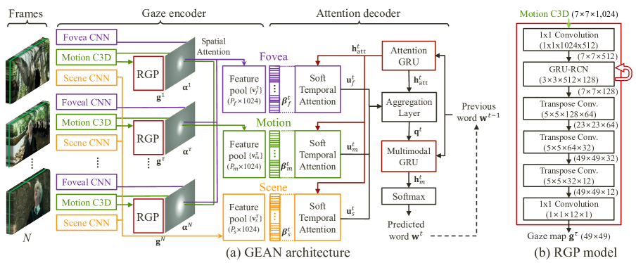
Figure 1: Illustration of the proposed Gaze Encoding Attention Network (GEAN) architecture. After extracting three types of CNN features per frame, the encoder generates pools of visual features using content and motion in videos, weighted by the spatial attention that the recurrent gaze prediction (RGP) model generates. The decoder generates word sequences by sequentially focusing on the most relevant subsets of the feature pools. In the RGP model, we present filter sizes inside boxes, and output dimensions next to arrows.

3.3 Construction of Visual Feature Pools

We construct three types of feature pools using the features of scene, motion, and fovea discussed in section 3.1. The first feature pool denoted by $\{\mathbf{v}_{s}^{\tau}\}_{\tau=1}^{N}$ is a simple collection of scene features for each frame, where $\tau$ is the frame index from 1 to $N$. For the next two feature pools, we use the predicted gaze map as spatial attention weights. Its underlying rationale is that human perceives focused regions in a high visual acuity with more neurons, while peripheral scene fields in a low resolution with less neurons [13]. Roughly simulating such a mechanism occurring in a focused foveal zone in human’s retina, we obtain a spatial attention map $\boldsymbol{\alpha}^{\tau}\in\mathbb{R}^{7\times 7}$ by average-pooling $\mathbf{g}^{\tau}\in\mathbb{R}^{49\times 49}$ with a $(7\times 7)$ kernel, and adding a uniform distribution with a strength of $\lambda$. Our empirical finding is that adding a uniform distribution leads to better performance; relying on only a very focused region can be risky to ignore too much relevant parts in the scene. We use $\lambda=0.6$ via cross validation. Finally, we $\ell_{1}$-normalize $\boldsymbol{\alpha}^{\tau}$ to yield a probability map. Next we define the motion and fovea feature pools (i.e. $\{\mathbf{v}_{m}^{\tau}\}_{\tau=1}^{N}$ and $\{\mathbf{v}_{f}^{\tau}\}_{\tau=1}^{N}$) as follows. We compute each $\mathbf{v}_{m}^{\tau}$ / $\mathbf{v}_{f}^{\tau}$ at frame $\tau$ as a weighted sum of element-wise dot-product between $\boldsymbol{\alpha}^{\tau}$ and the motion/fovea features, both of which have dimension of $(7\times 7\times 1,024)$ as presented in section 3.1. For example, each $\mathbf{v}_{m}^{\tau}\in\mathbb{R}^{1,024}$ is computed as $\mathbf{v}_{m}^{\tau}(k)=\sum_{i=1}^{7}\sum_{j=1}^{7}\boldsymbol{\alpha}^{\tau}(i,j)\mathbf{f}_{m}^{\tau}(i,j,k)$, where $\mathbf{f}_{m}^{\tau}$ is the C3D conv5b motion feature at frame $\tau$.

We then set the maximum lengths of pools denoted by $N_{max}$ for scene, motion, and attention features to 20, 35, and 35 respectively, based on the average length of video clips. If $N<N_{max}$, we repeat padding again from the feature of the first frame; otherwise, we uniformly sample frames to be fit to the limit length. We use a smaller pool size $P$ for the scene, because its variation across a clip is smaller than other feature types. We remind that all pooled features have a dimension of $1,024$.

3.4 The Decoder for Caption Generation

Our decoder for caption generation is designed based on the soft attention mechanism [2], which has been also applied in video captioning applications (e.g. [15, 36]). Thus, the decoder sequentially generates words by selectively weighting on different features in the three pools at each time. As shown in Fig.1, the decoder consists of a temporal attention module, an attention GRU, an aggregation layer, and a multimodal GRU.

Temporal attention module. For each feature pool $\{\mathbf{v}^{\tau}\}_{\tau}$, we compute a set of attention weights $\{\{\beta_{\tau}^{1}\}_{\tau},\cdots,\{\beta^{L}_{\tau}\}_{\tau}\}$ such that $\sum_{\tau=1}^{N}\beta_{\tau}^{t}=1$ at each time step $t$, where $N$ is the length of each visual pool, and $L$ is the output sentence length. Here $t$ indicates the step for a output word sequence; it is different with $\tau$ in the previous section, which means the frame index. Thus for each word $t$, the distribution $\{\beta_{\tau}^{t}\}_{\tau}$ determines the temporal attention. Since we have three sets of visual pools $\{\mathbf{v}_{s,m,f}^{\tau}\}_{\tau}$, we also have three sets of attention weights $\{\beta\}$. We let the attention mechanism for each pool to be independent; we below drop the subscript $s,m,f$ for simplicity. We compute a single aggregated feature vector $\mathbf{u}^{t}\in\mathbb{R}^{1,024}$ by $\beta$-weighted averaging on all the features $\{\mathbf{v}^{\tau}\}_{\tau}$ in each pool:

$$\mathbf{u}^{t} =\sum^{N}_{\tau=1}\beta^{t}_{\tau}\mathbf{v}^{\tau},\hskip 6.0pt\mbox{ where }\beta^{t}_{\tau}=\frac{\exp(q^{t}_{\tau})}{\sum_{\tau^{\prime}}\exp(q^{t}_{\tau^{\prime}})},\hskip 6.0pt$$ (5)

$$q^{t}_{\tau} =\mathbf{w}^{\top}\phi(\mathbf{W}_{q}\mathbf{v}^{\tau}+\mathbf{U}_{q}\mathbf{h}_{att}^{t}+\mathbf{b}_{q}),$$ (6)

where each attention weight $\beta^{t}_{\tau}$ is obtained by applying a sequential softmax to scalar attention scores $\{q_{\tau}^{t}\}_{\tau}$. The parameters includes $\mathbf{w}\in\mathbb{R}^{64\times 1}$, $\mathbf{W}_{q}\in\mathbb{R}^{64\times 1,024}$, $\mathbf{U}_{q}\in\mathbb{R}^{64\times 512}$ are shared for each feature pool at all time steps. The activation $\phi$ is a scaled hyperbolic tangent function (i.e. $\mathrm{stanh}(x)=1.7159\cdot\mathrm{tanh}(2x/3)$), and $\mathbf{h}_{att}^{t-1}\in\mathbb{R}^{512}$ is the previous hidden state of the attention GRU, which will be discussed below.

Attention GRU. Our attention GRU has the same form with the normal GRU [5] as follows:

$$\mathbf{z}_{att}^{t} =\sigma(\mathbf{W}_{z}\mathbf{x}_{att}^{t}+\mathbf{U}_{z}\mathbf{h}_{att}^{t-1}+\mathbf{b}_{z}),$$ (7)

$$\mathbf{r}_{att}^{t} =\sigma(\mathbf{W}_{r}\mathbf{x}_{att}^{t}+\mathbf{U}_{r}\mathbf{h}_{att}^{t-1}+\mathbf{b}_{r}),$$ (8)

$$\tilde{\mathbf{h}}_{att}^{t} =\mathrm{tanh}(\mathbf{W}_{h}\mathbf{x}_{att}^{t}+\mathbf{U}_{h}*(\mathbf{r}_{att}^{t}\odot\mathbf{h}_{att}^{t-1})),$$ (9)

$$\mathbf{h}_{att}^{t} =(1-\mathbf{z}_{att}^{t})\odot\mathbf{h}_{att}^{t-1}+\mathbf{z}_{att}^{t}\odot\tilde{\mathbf{h}}_{att}^{t}.$$ (10)

The input $\mathbf{x}_{att}^{t}$ is an embedding of the previous word: $\mathbf{x}_{att}^{t}=\mathbf{B}\mathbf{w}^{t-1}$, where $\mathbf{w}^{t-1}$ is a $V\times 1$ one-hot vector, and $\mathbf{B}\in\mathbb{R}^{512\times V}$ is a word embedding parameter. The hidden state representation $\mathbf{h}_{att}^{t}$ is the input to both the temporal attention module and the aggregation layer; that is, it influences not only the attention on the feature pools but also the generation of a next probable word.

Aggregation layer. Note that the attention feature vectors in Eq.(5) are obtained for each channel of scene, motion, and fovea separately: $\mathbf{u}_{s}^{t}$, $\mathbf{u}_{m}^{t}$, and $\mathbf{u}_{f}^{t}$, which are then fed into the aggregation layer.

$$\mathbf{q}^{t}=\phi(([\mathbf{W}_{g}^{s}\mathbf{u}_{s}^{t}\parallel\mathbf{W}_{g}^{m}\mathbf{u}_{m}^{t}\parallel\mathbf{W}_{g}^{f}\mathbf{u}_{f}^{t}]+\mathbf{b}_{g})\odot\mathbf{U}_{g}\mathbf{h}_{att}^{t})$$ (11)

where $\parallel$ denotes the vector concatenation, and parameters include $\mathbf{W}_{g}^{s}\in\mathbb{R}^{256\times 1,024},\mathbf{W}_{g}^{m}\in\mathbb{R}^{256\times 1,024},\mathbf{W}_{g}^{f}\in\mathbb{R}^{512\times 1,024},\mathbf{b}_{m}\in\mathbb{R}^{1,024\times 1}$ and $\mathbf{U}_{g}\in\mathbb{R}^{1,024\times 512}$. We apply a dropout regularization [28] with a rate of 0.5 to the aggregation layer, which mixes each feature channel representation with previous word information via the hidden state $\mathbf{h}_{att}^{t}$ of the attention GRU. It then outputs a vector $\mathbf{q}^{t}\in\mathbb{R}^{1,024}$, based on which the multimodal GRU generates a next likely word.

Multimodal GRU. The multimodal GRU has the same structure with the attention GRU with only difference that input $\mathbf{x}_{m}^{t}$ is a concatenation of the output of the aggregation layer and the previous word embedding: $[\mathbf{q}^{t},\mathbf{B}\mathbf{w}^{t-1}]\in\mathbb{R}^{1,536}$. That is, the multimodal GRU couples attended visual features with embedding of the previous word. The hidden state $\mathbf{h}_{m}^{t}$ is fed into a softmax layer over all the words in the dictionary to predict the index of a next word:

$$p(\mathbf{w}^{t}\mid\mathbf{w}^{1:t-1})=\mathrm{softmax}(\mathbf{W}_{out}\mathbf{h}_{m}^{t}+\mathbf{b}_{h}),$$ (12)

where parameters include $\mathbf{W}_{out}\in\mathbb{R}^{V\times 512}$ and $\mathbf{b}_{h}\in\mathbb{R}^{V\times 1}$. We use a greedy decoding scheme to choose the best word $\mathbf{w}^{t}$ that maximizes Eq.(12) at each time step.

Spatial and temporal Attention. The proposed GEAN model leverages both spatial and temporal attention. The spatial attention is used for generating feature pools that are weighted by gaze maps predicted by the RGP model. The temporal attention is used for selecting a subset of feature pools for word generation by modules in the decoder. By sequentially running the two attentions, we can significantly reduce the dimensionality of spatio-temporal attention compared to other previous work (e.g. [27, 36]), which allows us to train the model with fewer training data. Moreover, it also resembles human’s perceptual process that is initially sensitive to visual stimuli, and then creates words using the memory about visual experience.

3.5 Training

We first train the RGP model, and then learn the entire GEAN model while fixing parameters of the RGP model. This two-step learning leads to better performance than allowing parameter update.

Training of the RGP model. We obtain groundtruths of gaze maps from human gaze tracking data in the training sets of VAS and Hollywood2. Following [18], we first build a ($49\times 49$) binary fixation map from raw gaze data, and then apply Gaussian filtering with $\sigma=2.0$ and $\ell_{1}$-normalization to obtain a ($49\times 49$) groundtruth gaze map, which can be seen as a valid probability distribution of eye fixation. We use the averaged frame-wise cross-entropy loss between predicted and GT gaze maps. We minimize the loss with Adam optimizer [12], with an initial learning rate of $10^{-4}$. To reduce overfitting further, we use data augmentation of image mirroring.

Training of the GEAN model. We limit the maximum length $L$ of training sentences to 80 words. We use the cross-entropy loss between predicted and GT words with $\ell_{2}$-regularization to avoid overfitting. We use orthogonal random initialization for two GRUs, and Xavier initialization [8] for convolutional and embedding layers. We use Adam optimizer [12] with an initial learning rate of $10^{-4}$.

4 Experiments

We first validate the performance of the recurrent gaze prediction (RGP) model for gaze prediction in section 4.1 We then report quantitative results of human gaze supervision on the attention-based captioning in section 4.2. Finally, we present AMT-based human assessment results for captioning quality in section 4.3. We defer more thorough experimental results to the supplementary. We plan to make public our source code and VAS dataset.

For evaluation, we randomly split VAS dataset into 60/40% as training and test sets. For LSMDC and Hollywood2 dataset, we use the split provided by original papers [24] and [18], respectively.

4.1 Evaluation of Gaze Prediction

	VAS				Hollywood2 EM
Metrics	Sim	CC	sAUC	AUC	Sim	CC	sAUC	AUC
ShallowNet [19]	0.361	0.407	0.498	0.821	0.369	0.433	0.501	0.855
ShallowNet+GRU	0.338	0.414	0.495	0.856	0.350	0.438	0.508	0.884
C3D+Conv	0.347	0.399	0.643	0.860	0.445	0.561	0.663	0.907
C3D+GRU	0.344	0.425	0.507	0.861	0.466	0.554	0.570	0.909
RGP (Ours)	0.483	0.586	0.702	0.912	0.478	0.588	0.682	0.924

Table 2: Evaluation of gaze prediction on the VAS and Hollywood 2 dataset.

Method	Random Uniform	Central Bias [18]	SF+MF+CB [18]	Human [18]	RGP (Ours)
AUC	0.500	0.840	0.871	0.936	0.924

Table 3: Gaze prediction results in terms of AUC for Hollywood2 dataset.

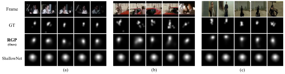
Figure 2: Examples of gaze prediction for video clips of Hollywood2 in (a–b) and VAS in (c). In each set, we show five representative frames of the clip, along with GTs and predicted gaze maps predicted by different methods.

We evaluate gaze prediction performance by measuring similarities between the predicted and groundtruth (GT) gaze maps of test sets. We follow the evaluation protocol of [10, 18, 19]. Each algorithm predicts a ($49\times 49$) gaze map for each frame, to which we apply Gaussian filtering with $\sigma=2.0$. We then upsample it to the original frame size using bilinear interpolation. The GT gaze map is obtained by averaging multiple subjects’ fixation points, followed by a Gaussian filtering with $\sigma=19$. After min-max normalization of predicted and GT gaze maps in a range of $[0,1]$, we compute performance metrics averaged over all the frames of each test clip. The performance measures include the similarity metric (Sim), linear correlation coefficient (CC), shuffled AUC (sAUC) and Judd implementation of AUC (AUC), whose details can be found in [21]. To compare with the results in [18], we follow the evaluation procedure of [18]; we uniformly sample 10 sets of 3,000 frames from test video clips, and report averaged performance.

Baselines. The ShallowNet [19] is one of the state-of-the-art methods for saliency or fixation prediction. Since it is designed for images not for videos, we test two different versions; we separately apply it to individual frames, denoted by (ShallowNet), and integrate it with the GRU [5] for sequence prediction, denoted by (ShallowNet+GRU). We also experiment two variants of our model to validate the effects of the recurrent component; (C3D+Conv) is our (RGP) excluding the GRU-RCN part, and (C3D+GRU) replaces the recurrent structure with vanilla GRU.

Quantitative results. Table 3 reports gaze prediction results of multiple models on VAS and Hollywood2 EM datasets. The variants of ShallowNets do not accurately capture human gaze sequences, and even with the recurrent model of (ShallowNet+GRU). Thanks to the representative power of the C3D motion feature and effectiveness of our recurrent model, the proposed (RGP) model significantly outperforms all the baselines in all evaluation metrics with large margins. Another advantage of the RGP model is that it needs relatively fewer parameters compared to other baselines, being beneficial for integrating with video captioning models without a risk of overfitting. Table 3 compares our results with the best results of Hollywood2 reported in [18] in terms of the AUC metric. Our AUC of 0.924 is significantly higher than the best reported AUC of 0.871 in [18], only slightly worsen than the human level of 0.936. For VAS evaluation, we train models using the combined training set from VAS and Hollywood2, because the VAS dataset size is relatively small. For Hollywood2 evaluation, we use Hollywood2 training data only to fairly compare with the results of [18].

Qualitative results. Fig.2 presents comparison of gaze prediction results between different methods and GTs on VAS and Hollywood2 datasets. While the baselines, including (ShallowNet) and (ShallowNet+GRU), do not correctly localize the gaze point with a bias toward the center. On the other hand, our model can effectively localize gaze points over frame sequences.

4.2 Evaluation of Video Captioning

Dataset	VAS						LSMDC
Language metrics	B1	B2	B3	M	R	Cr	B1	B2	B3	M	R	Cr
No spatial attention by gaze maps (i.e. without RGP)
Temp-Attention [15]	0.139	0.049	0.028	0.039	0.124	0.035	0.082	0.028	0.009	0.043	0.117	0.047
S2VT+VGG16 [33]	0.241	0.091	0.051	0.068	0.195	0.060	0.162	0.051	0.017	0.070	0.157	0.088
S2VT+GNet [33]	0.233	0.088	0.043	0.069	0.189	0.058	0.142	0.041	0.015	0.065	0.153	0.083
h-RNN+GNet+C3D [36]	0.255	0.099	0.038	0.067	0.181	0.055	0.128	0.038	0.011	0.066	0.156	0.070
GEAN+GNet	0.259	0.102	0.041	0.068	0.196	0.057	0.154	0.050	0.016	0.067	0.153	0.091
GEAN+GNet+C3D	0.264	0.105	0.042	0.070	0.201	0.058	0.166	0.050	0.018	0.068	0.154	0.095
GEAN+GNet+C3D+Scene	0.274	0.118	0.046	0.075	0.211	0.080	0.166	0.050	0.018	0.069	0.157	0.084
Spatial attention by RGP predicted gaze maps (i.e. with RGP)
Temp-Attention [15]	0.147	0.049	0.029	0.046	0.149	0.048	0.085	0.028	0.011	0.046	0.121	0.057
S2VT+GNet [33]	0.268	0.101	0.044	0.073	0.199	0.069	0.131	0.038	0.013	0.066	0.153	0.080
h-RNN+GNet+C3D [36]	0.273	0.101	0.045	0.073	0.196	0.073	0.146	0.046	0.017	0.067	0.151	0.074
GEAN+GNet	0.282	0.119	0.049	0.077	0.209	0.075	0.152	0.051	0.016	0.068	0.152	0.081
GEAN+GNet+C3D+Scene	0.306	0.125	0.049	0.084	0.229	0.084	0.168	0.055	0.021	0.072	0.156	0.093

Table 4: Evaluation of video captioning with or without the RGP model for VAS and LSMDC datasets. For language metrics, we use BLEU (B), METEOR (M), ROUGE (R), and CIDEr (Cr), in all of which higher is better.

Dataset	(GEAN) w/ RGP	Uniform	Random Gaze	Central Gaze	Peripheral Gaze
LSMDC	0.072	0.069	0.056	0.061	0.057
VAS	0.084	0.075	0.062	0.073	0.068

Table 5: METEOR score comparison between learned and various fixed gaze weights.

In previous section, we validate that the proposed gaze prediction achieves state-of-the-art performances. Based on such dependably predicted gaze maps, we test how much they help improve attention-based captioning models. For evaluation, each video captioning method predicts a sentence for a test video clip, and we measure the performance by comparing between its prediction and the groundtruth sentence. We use four different language similarity metrics, BLEU [20], METEOR [14], ROUGE [16] and CIDEr [32].

Baselines. We compare with four state-of-the-art video captioning methods. First, (Temp-Attention) [15] is one of the first soft temporal attention models for video captioning. Second, the S2VT [33] is a sequence-to-sequence model that directly learns mappings between frame sequences to word sequences. We test two variants denoted by (S2VT+VGG16) and (S2VT+GNet) according to frame representation VGGNet-16 and GoogLeNet. Finally, (h-RNN+GNet) [36] is a hierarchical RNN model that also leverages a soft attention scheme to generate multiple sentences. For (Temp-Attention), we use the source code proposed by original authors. For (S2VT+*), we transform the original Caffe code into TensorFlow, in order to integrate with the gaze prediction module. We implement (h-RNN+*) by ourselves because no code is available.

(GEAN) w/ RGP vs	(S2VT) w/ RGP	(h-RNN) w/ RGP	(Temp-Attention) w/ RGP
LSMDC	58.7 % (176/300)	59.3 % (178/300)	73.7 % (221/300)
VAS	61.0 % (183/300)	69.7 % (209/300)	76.7 % (230/300)

Table 6: The results of Amazon Mechanical Turk (AMT) pairwise preference tests on LSMDC and VAS datasets. We present the percentages of responses that turkers vote for (GEAN) w/ RGP against baselines with RGP.

	(GEAN)	(S2VT)	(h-RNN)	(Temp-Attention)
LSMDC	65.3 % (196/300)	58.0 % (174/300)	59.7 % (179/300)	60.7 % (182/300)
VAS	67.0 % (201/300)	60.7 % (182/300)	62.7 % (188/300)	63.3 % (190/300)

Table 7: The results of AMT pairwise preference tests between the models with or without RGP. For example, the second column shows the percentages of Turkers’ votes for (S2VT) with RGP against (S2VT) without RGP.

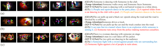
Figure 3: Video captioning examples of (a) correct, (b) relevant, and (c) incorrect descriptions. In every frame, we present groundtruth (GT) human eye fixation with colored circles, and gaze prediction with white for attended regions. We show captions predicted by different methods along with GTs. We present more, clearer, and larger examples in the supplementary.

Quantitative results. Table 5 shows quantitative results of different methods for video captioning. We also run multiple variants of our GEAN model denoted by (GEAN+*) according to different feature combinations. We perform two sets of experiments with or without using the spatial attention by gaze maps that the RGP model predicts. The baselines without the RGP model means that they are executed as originally proposed. For fair comparison, we use GoogLeNet inception5b layers as features for all baselines except (S2VT+VGG16). We obtain the results of (S2VT+VGG16) for LSMDC dataset from the leaderboard of the LSMDC challenge. Except this, we generate all the results by ourselves.

We summarize some experimental consequences as follows. First, the proposed GEAN models achieve the best performance in each group of experiments for both datasets and with or without the RGP model. Second, we observe that the performance of most methods increases with using spatial attention by gaze maps that the RGP predicts, although the GEAN methods benefit the most from gaze prediction. Such improvement is less significant in LSMDC than VAS dataset, mainly because LSMDC has no gaze tracking data for training. We remind that the RGP model is trained with VAS and Hollywood2 datasets. Finally, experiments assure that it is the best for the GEAN model to use all the three visual feature pools, as (GEAN+GNet+C3D+Scene) attains the highest values in all the four groups of experiments.

Effects of different gaze weights. Table 5 compares captioning performance between different gaze weights within the RGP module. For brief comparison, we report only METEOR scores. In the table, the performance with learned gazes by our model comes in the first column, and those of other baselines follow. The uniform gaze assigns a uniform $1/49$ weight to $7\times 7$ grid. The random gaze selects a single bin randomly, while the central gaze picks the center $(4,4)$ bin in the grid. Then, those one hot matrices of random and central gaze are smoothed by Gaussian filtering with $\sigma=1.0$. Finally, the peripheral gaze is an $\ell_{1}$-normalized inverse of the central gaze. As shown in Table 5, the learned gaze by our model leads the best captioning performance. Among the fixed gaze weights, the uniform gaze is the best, which hints that it is better using the whole scene than attending on wrong parts of the scene.

Qualitative results. Fig.3 shows three examples of video captioning results for (a) correct description, (b) relevant description, and (c) incorrect description. In frames, we present GT human eye fixation with colored circles, and gaze prediction with white for attended regions. We also show the captions predicted by different methods along with GTs. We observe that the spatial attention predicted by our method matches well with GT human eye fixation, and description generated by our method are more accurate than the baselines. We present more, clearer, and larger examples in the supplementary.

4.3 Human Evaluation via AMT

We perform user studies using Amazon Mechanical Turk (AMT) to observe general users’ preferences on the generated descriptions. We conduct pairwise comparison (A/B Test); in each AMT task, we show a clip and two captions generated by different methods in a random order, and ask turkers to pick a better one without knowing which comes from which methods. For test cases, we randomly sample 100 examples each from LSMDC and VAS datasets. We collect answers from three turkers for each test case.

Table 6 shows the results of AMT tests on LSMDC and VAS datasets, in which we compare our (GEAN) with the RGP model against the baselines with the RGP, including (h-RNN), (S2VT), and (Temp-Attention). We observe that general AMT turkers prefer output sentences of our approach to those of baselines. Those response margins are more significant than language metric differences.

Table 7 summarizes the results of AMT tests between the methods with or without RGP. That is, for both our model and other baselines, we evaluate how much the gaze prediction by the RGP improves the caption qualities perceived by general users. Consequently, even baselines with the RGP model obtains more votes than those without RGP. It can be another evidence that gaze supervision helps even baselines to produce better descriptive sentences.

5 Conclusion

We proposed the Gaze Encoding Attention Network (GEAN) that leverage human gaze data to supervise attention-based video captioning. With experiments and user studies on our newly collected VAS, caption-only LSMDC, and gaze-only Hollywood2 datasets, we showed that multiple attention-based captioning methods benefit from gaze information to attain better captioning quality. We also demonstrated the GEAN model outperforms the state-of-the-art video captioning alternatives.

Acknowledgements. This research is partially supported by Convergence Research Center through National Research Foundation of Korea (2015R1A5A7037676). Gunhee Kim is the corresponding author.

See pages 1 of cvpr17_gaze_supp.pdf See pages 2 of cvpr17_gaze_supp.pdf See pages 3 of cvpr17_gaze_supp.pdf See pages 4 of cvpr17_gaze_supp.pdf See pages 5 of cvpr17_gaze_supp.pdf See pages 6 of cvpr17_gaze_supp.pdf See pages 7 of cvpr17_gaze_supp.pdf See pages 8 of cvpr17_gaze_supp.pdf See pages 9 of cvpr17_gaze_supp.pdf See pages 10 of cvpr17_gaze_supp.pdf See pages 11 of cvpr17_gaze_supp.pdf See pages 12 of cvpr17_gaze_supp.pdf See pages 13 of cvpr17_gaze_supp.pdf See pages 14 of cvpr17_gaze_supp.pdf See pages 15 of cvpr17_gaze_supp.pdf See pages 16 of cvpr17_gaze_supp.pdf See pages 17 of cvpr17_gaze_supp.pdf

References

- [1] J. Ba, V. Mnih, and K. Kavukcuoglu. Multiple Object Recognition with Visual Attention. In ICLR, 2015.
- [2] D. Bahdanau, K. Cho, and Y. Bengio. Neural Machine Translation by Jointly Learning to Align and Translate. In ICLR, 2015.
- [3] N. Ballas, L. Yao, C. Pal, and A. C. Courville. Delving Deeper into Convolutional Networks for Learning Video Representations. In ICLR, 2016.
- [4] S. Bird, E. Loper, and E. Klein. Natural Language Processing with Python. O’Reilly Media Inc., 2009.
- [5] K. Cho, B. Van Merrienboer, C. Gulçehre, D. Bahdanau, F. Bougares, H. Schwenk, and Y. Bengio. Learning Phrase Representations using RNN Encoder–Decoder for Statistical Machine Translation. In EMNLP, 2014.
- [6] P. Das, C. Xu, R. F. Doell, and J. J. Corso. A Thousand Frames in Just a Few Words: Lingual Description of Videos through Latent Topics and Sparse Object Stitching. In CVPR, 2013.
- [7] J. Donahue, L. A. Hendricks, S. Guadarrama, M. Rohrbach, S. Venugopalan, K. Saenko, and T. Darrell. Long-term Recurrent Convolutional Networks for Visual Recognition and Description. In CVPR, 2015.
- [8] X. Glorot and Y. Bengio. Understanding the difficulty of training deep feedforward neural networks. In AISTATS, 2010.
- [9] S. Guadarrama, N. Krishnamoorthy, G. Malkarnenkar, S. Venugopalan, R. Mooney, T. Darrell, and K. Saenko. YouTube2Text: Recognizing and Describing Arbitrary Activities Using Semantic Hierarchies and Zero-shot Recognition. In ICCV, 2013.
- [10] M. Jiang, S. Huang, J. Duan, and Q. Zhao. SALICON: Saliency in Context. In CVPR, 2015.
- [11] A. Karpathy, G. Toderici, S. Shetty, T. Leung, R. Sukthankar, and L. Fei-Fei. Large-scale video classification with convolutional neural networks. In CVPR, 2014.
- [12] D. Kingma and J. Ba. Adam: A method for stochastic optimization. In ICLR, 2015.
- [13] A. M. Larson and L. C. Loschky. The contributions of central versus peripheral vision to scene gist recognition. Journal of Vision, 2009.
- [14] S. B. A. Lavie. METEOR: An Automatic Metric for MT Evaluation with Improved Correlation with Human Judgments. In ACL, 2005.
- [15] Y. Li, T. Atousa, C. Kyunghyun, B. Nicolas, P. Christopher, L. Hugo, and C. Aaron. Describing Videos by Exploiting Temporal Structure. In ICCV, 2015.
- [16] C.-Y. Lin. ROUGE: A Package for Automatic Evaluation of Summaries. In WAS, 2004.
- [17] M. Marszałek, I. Laptev, and C. Schmid. Actions in context. In CVPR, 2009.
- [18] S. Mathe and C. Sminchisescu. Actions in the Eye: Dynamic Gaze Datasets and Learnt Saliency Models for Visual Recognition. IEEE PAMI, 37:1408–1424, 2015.
- [19] J. Pan, K. McGuinness, E. Sayrol, N. O’Connor, and X. Giro-i Nieto. Shallow and Deep Convolutional Networks for Saliency Prediction. In CVPR, 2016.
- [20] K. Papineni, S. Roukos, T. Ward, and W.-J. Zhu. BLEU: A Method for Automatic Evaluation of Machine Translation. In ACL, 2002.
- [21] N. Riche, M. Duvinage, M. Mancas, B. Gosselin, and T. Dutoit. Saliency and Human Fixations: State-of-the-art and Study of Comparison Metrics. In ICCV, 2013.
- [22] A. Rohrbach, M. Rohrbach, and B. Schiele. The long-short story of movie description. In GCPR, 2015.
- [23] A. Rohrbach, M. Rohrbach, N. Tandon, and B. Schiele. A Dataset for Movie Description. In CVPR, 2015.
- [24] A. Rohrbach, A. Torabi, M. Rohrbach, N. Tandon, C. Pal, H. Larochelle, A. Courville, and B. Schiele. Movie Description. IJCV, 2017.
- [25] M. Rohrbach, W. Qiu, I. Titov, S. Thater, M. Pinkal, and B. Schiele. Translating Video Content to Natural Language Descriptions. In ICCV, 2013.
- [26] O. Russakovsky, J. Deng, H. Su, J. Krause, S. Satheesh, S. Ma, Z. Huang, A. Karpathy, A. Khosla, M. Bernstein, A. C. Berg, and L. Fei-Fei. Imagenet large scale visual recognition challenge. IJCV, 2015.
- [27] S. Sharma, R. Kiros, and R. Salakhutdinov. Action Recognition Using Visual Attention. In ICLR Workshop, 2016.
- [28] N. Srivastava, G. Hinton, A. Krizhevsky, I. Sutskever, and R. Salakhutdinov. Dropout: A simple way to prevent neural networks from overfitting. JMLR, 2014.
- [29] C. Szegedy, W. Liu, Y. Jia, P. Sermanet, S. Reed, D. Anguelov, D. Erhan, V. Vanhoucke, and A. Rabinovich. Going deeper with convolutions. In CVPR, 2015.
- [30] A. Torabi, P. Chris, L. Hugo, and C. Aaron. Using Descriptive Video Services to Create a Large Data Source for Video Annotation Research. arXiv:1503.01070, 2015.
- [31] D. Tran, L. Bourdev, R. Fergus, L. Torresani, and M. Paluri. Learning Spatiotemporal Features with 3D Convolutional Networks. In ICCV, 2015.
- [32] R. Vedantam, C. L. Zitnick, and D. Parikh. CIDEr: Consensus-based Image Description Evaluation. In CVPR, 2015.
- [33] S. Venugopalan, R. Marcus, D. Jeffrey, M. Raymond, D. Trevor, and S. Kate. Sequence to Sequence - Video to Text. In ICCV, 2015.
- [34] S. Venugopalan, H. Xu, J. Donahue, M. Rohrbach, R. Mooney, and K. Saenko. Translating Videos to Natural Language Using Deep Recurrent Neural Networks. In HLT-NAACL, 2015.
- [35] K. Xu, J. Ba, R. Kiros, A. Courville, R. Salakhutdinov, R. Zemel, and Y. Bengio. Show, Attend and Tell: Neural Image Caption Generation with Visual Attention. In ICML, 2015.
- [36] H. Yu, J. Wang, Z. Huang, Y. Yang, and W. Xu. Video Paragraph Captioning Using Hierarchical Recurrent Neural Networks. In CVPR, 2016.
- [37] B. Zhou, A. Lapedriza, J. Xiao, A. Torralba, and A. Oliva. Learning deep features for scene recognition using places database. In NIPS, 2014.