Dynamical System Analysis of Interacting Hessence Dark Energy in $f(T)$ Gravity

Abstract

In this work, we have carried on dynamical system analysis of hessence field coupling with dark matter in $f(T)$ gravity. We have analysed the critical points due to autonomous system. The resulting autonomous system is non-linear. So, we have approached via the the theory of non-linear dynamical system. We have noticed very few papers are devoted to this kind of study. Maximum works in literature are done treating the dynamical system as done in linear dynamical analysis, which are unable to predict correct evolution. Our work is totally different from those kind of works. We have used theory of non-linear dynamical system theory, developed till date, in our analysis. This approach gives totally different stable solutions, in contrast what the linear analysis would have predicted. We have discussed the stability analysis in details due to exponential potential through computational method in tabular form and analyzed the evolution of the universe. Some plots are drawn to investigate the behaviour of the system (this plotting technique is different from usual phase plot and devised by us). Interestingly, the analysis shows the universe may resemble the ‘cosmological constant’ like evolution (i.e., $\Lambda$CDM model is a subset of the solution set). Also, all the fixed points of our model are able to avoid Big rip singularity.

1 Introduction

High end cosmological observations of the Supernova of type Ia (SN Ia), WMAP, etc., [1, 2, 3, 4, 5, 6, 7, 8, 9, 10, 11, 12, 13, 14, 15, 16, 17, 18, 19] suggest the fact that the universe may be accelerating lately again after the early phase. Many theories are formulated to explain this late time acceleration. However, these theories can be divided mainly in two categories fulfilling the criteria of a homogeneous and isotropic universe. First kind of theory (better to known as ‘Standard model’ or $\Lambda$CDM model) assumes a fluid of negative pressure named as ‘dark energy’ (DE). The name arises from the fact the exact origin of this energy is still unexplained in theoretical set up. Observations, anyway, indicate nearly 70$\%$ of the universe may be occupied by this kind of energy. Dust matter (cold dark matter (CDM) and baryon matter) comprises the rest 30$\%$ and there is negligible radiation. Cosmologists are inclined to suspect dark energy as the primal cause of the late acceleration of universe. Theory of dark energy has remained one of the foremost area of research in cosmology till the discovery of acceleration of the universe at late times [20, 21, 22, 23, 24, 25]. One could clearly notice from the second field equation, that the expansion would be accelerated if the equation of state (EoS) parameter satisfies, $p/{\rho}{\equiv}{\omega}<-1/3$. Accordingly, then a priori choice for dark energy is a time independent positive ‘cosmological constant’ which relates to the equation of state (EoS) $\omega=-1$. This gives an universe which is expanding forever at exponential rate. Anyway, cosmological constant has some severe shortcomings like fine tuning problem etc (see[20] for a review), some recent data [26, 27] in some sense, agrees with this choice. By the way, observations which constrains $\omega$ close to the value of cosmological constant, of $\omega$ does not indicate whether $\omega$ changes with time or not. So theoretically, one could consider $\omega$ as a function of cosmic time, such as inflationary cosmology (see [28, 29, 30, 31, 32] for review). Scalar fields evolve in particle physics quite naturally. Till date, a large variety of scalar field inflationary models are discussed. This theory is active area in literature nowadays (see [20]). The scalar field which lightly interacts with gravity is called ‘quintessence’. Quintessence fields are first hand choice because this field can lessen fine tuning problem of cosmological constant to some extent. Needless to say, some common drawback for quintessence are also there. Observations point that at current epoch energy density of scalar field and matter energy density is comparable. But, we know they evolve from different initial conditions. This discrepancy (known as ‘coincidence problem’) arises for any scalar field dark energy, quintessence too suffer from this problem [33]. Of course, there is resolution of this problem, they are called ‘tracking solution’ [34]. In the tracking regime, field value should be of the order of Planck mass. Anyway a general setback is that we always need to seek for such potentials (see [35] for related discussion). Eos parameter $\omega$ of quintessence satisfies $-1{\leq}\omega{\leq}1$. Some current data indicates that $\omega$ lies in small neighbourhood of $\omega=-1$. Hence it is technically feasible to relax $\omega$ to go down the line $\omega<-1$ [36]. There exists another scalar field with negative kinetic energy term,which can describe late acceleration. This is named as phantom field, which has Eos $\omega<-1$ (see details in [20, 37]). Phantom field energy density increases with time. As a result, Hubble factor and curvature diverges in finite time causing ‘Big-rip’ singularity (see [38, 39, 40]). By the way, some specific choice of potential can avoid this flaw. Present data perhaps favours a dark energy model with $\omega>-1$ of recent past to $\omega<-1$ at present time [41]. The line $\omega=-1$ is known as ‘phantom’ divide. Evidently, neither quintessence nor phantom field alone can cross the phantom divide. In this direction, a firsthand choice is to combine both quintessence and phantom field. This is known in the literature as ‘quintom’ (i.e., hybrid of quintessence and phantom) [41]. This can serve the purpose, but still has some fallacy. A single canonical complex field is quite natural and useful (like ‘spintessence’ model [42, 43]). However, canonical complex scalar fields suffer a serious setback, namely the formation of ‘Q-ball’ (a kind of stable non-topological soliton) [42, 43].

To overcome various difficulties with above mentioned models Wei et al in their paper [44, 45] introduced a non-canonical complex scalar field which plays the role of quintom [46, 47, 48]. They name this unique model as ‘hessence’. However, hessence is unlike other canonical complex scalar fields which suffer from the formation of Q-ball. Second kind of theory modifies the classical general relativity (GR) by higher degree curvature terms (namely, $f(R)$ theory) [49, 50, 51] or by replacing symmetric Levi-Civita connection in GR theory by antisymmetric Weitzenb$\ddot{o}$ck connection. In other words, torsion is taken for gravitational interaction instead of curvature. The resulting theory [52, 53, 54] (called ‘Teleparallel’ gravity) was considered initially by Einstein to unify gravity with electromagnetism in non-Riemannian Weitzenböck manifold. Later further modification done to obtain $f(T)$ gravity as in the same vein of $f(R)$ gravity theory [55]. Although,the Eos of ‘cosmological constant’ ($\Lambda$CDM model) is well within the various dataset, till now not a single observation can detect DE or DM, and search for possible alternative are on their way [56]. In this regard alternate gravity theory (like, $f(T)$) really worth discussing. The work [57] is a nice account in establishing matter stability of $f(T)$ theory in weak field limit in contrast to $f(R)$ theory. It is shown that any choice of $f(T)$ can be used.Other reason for the theoretical advantage for their choice are discussed in the next section.

We, in this work have chosen hessence in $f(T)$ gravity. Since, the system is complex, we have preferred a dynamical analysis. As, we have mentioned previously hessence field and $f(T)$ theory both are promising candidates to explain present accelerated phase. So, we merged them to find if they can highlight present acceleration more accurately with current dataset. A mixed dynamical system with tachyon, quintessence and phantom in $f(T)$ theory is considered in [58]. Dynamical systems with quintom are there in literature also (see [59, 60] for review). The dynamical system analysis for normal scalar field model in $f(T)$ gravity has been discussed in ref [61]. But, to the best of our knowledge hessence in $f(T)$ gravity is not considered before.

We arrange the paper in following manner. Short sketch of $f(T)$ theory is presented in section 2. Hessence field in $f(T)$ gravity is introduced to form dynamical system in section 3. Section 4 is devoted dynamical system analysing and the stability of the system for hessence dark energy model. The significance of our result is discussed in section 5 in light of recent data. We concluded the paper with relevant remarks in section 6. We use normalized units as $8\pi G={\hbar}=c=1$ in this paper.

2 A Brief Outline of $f(T)$ gravity: Some Basic Equations

In teleparallelism [55, 62, 63], $e^{\mu}_{A}$ are called the orthonormal tetrad components $(A=0,1,2,3)$. The index $A$ is used for each point $x^{\mu}$ for a tangent space of the manifold, hence each $e^{\mu}_{A}$ represents a tangent vector to the manifold (i.e., the so called vierbein). Also the inverse of the vierbein is obtained from the relation ${e^{\mu}_{A}}{e^{A}_{\nu}}=\delta^{\mu}_{\nu}$. The metric tensor is given as, $g_{\mu\nu}=\eta_{AB}{e^{A}_{\mu}}{e^{A}_{\nu}}$ ($\mu,\nu$=0,1,2,3),$\mu,\nu$ are coordinate indices on the manifold (here, $\eta_{AB}$=diag(1,-1,-1,-1)). Recently, to explain the acceleration the teleparallel torsion $(T)$ in Lagrangian density has been modified from linear torsion to some differentiable function of $T$ [64, 65] (i.e., $f(T)$) likewise $f(R)$ theory mentioned earlier. In this new set up of gravity the field equation is of second order unlike $f(R)$ (which is fourth order). In $f(T)$ theory of gravitation, corresponding action reads as,

$$\mathcal{A}=\frac{1}{2{\kappa^{2}}}\int{d^{4}x}[\sqrt{-g}(T+f(T))+\mathcal{L}_{m}]$$ (1)

where $T$ is the torsion scalar, $f(T)$ is some differentiable function of torsion $T$, $\mathcal{L}_{m}$ is the matter Lagrangian, $\sqrt{-g}=det(e^{A}_{\mu})$ and $\kappa^{2}=8\pi G$. The torsion scalar $T$ mentioned above is defined as,

$$T={S_{\rho}}^{\mu\nu}{T^{\rho}}_{\mu\nu}$$ (2)

with the components of torsion tensor ${T^{\rho}}_{\mu\nu}$ of (2) is given by,

$${T^{\rho}}_{\mu\nu}={{\Gamma^{W}}^{\lambda}}_{\nu\mu}-{{\Gamma^{W}}^{\lambda}}_{\mu\nu}={e^{\lambda}_{A}}({\partial_{\mu}}{e^{A}_{\nu}}-{\partial_{\nu}}{e^{A}_{\mu}})$$ (3)

where, ${{\Gamma^{W}}^{\lambda}}_{\nu\mu}={e^{\lambda}_{A}}{\partial_{\mu}}{e^{A}_{\nu}}$ is the Weitzenböck connexion. Here, The superpotential ${S_{\rho}}^{\mu\nu}$ (2) is defined as bellow,

$${S_{\rho}}^{\mu\nu}=\frac{1}{2}({K^{\mu\nu}}_{\rho}+{\delta^{\mu}_{\rho}}{T^{\theta\nu}}_{\theta}-{\delta^{\nu}_{\rho}}{T^{\theta\mu}}_{\theta})$$ (4)

$${K^{\mu\nu}}_{\rho}=(-)\frac{1}{2}({T^{\mu\nu}}_{\rho}-{T^{\nu\mu}}_{\rho}-{T_{\rho}}^{\mu\nu})$$ (5)

${K^{\mu\nu}}_{\rho}$ is called as contortion tensor. The contortion tensor measures the difference between symmetric Levi-Civita connection and anti-symmetric Weitzenböck conexion. It is easy to check that the equation of motion reduces to Einstein gravity if $f(T)=0$. Actually this is the correspondence between teleparallel and Einsteinian theory [54]. It is noticed that $f(T)$ theory can address early acceleration and late evolution of universe depending on the choice of $f(T)$. For example, power law or exponential form can’t overcome phantom divide [66], but some other choices of $f(T)$ [67] can cross phantom divide. The reconstruction of $f(T)$ model [68, 69], various cosmological [70, 71] and thermodynamical [72] analysis, has been reported. It is to interesting to note that linear $f(T)$ model (i.e., when $\frac{dF}{dT}=$ constant) behaves as cosmological constant. Anyway, a preferable choice of $f(T)$ is such that it reduces to General Relativity (GR) when redshift is large in tune with primordial nucleosynthesis and cosmic microwave data at early times (i.e., $f/T{\rightarrow}0$ for $a<<1$). Moreover, in future it should give de-Sitter like state. One such choice is given in power form as in [73], namely

$$f(T)=\beta{(-T)^{n}}$$ (6)

$\beta$ being a constant. In particular, $n=1/2$ gives same expanding model as the theory referred in [73, 74]. Current data needs the bound $`n<<1^{\prime}$ to permit $f(T)$ as an alternate gravity theory. The effective DE equation of state varies from $\omega=-1+n$ of past to $\omega=-1$ in future.

Throughout the work we assume flat, homogeneous, isotropic Friedman-Lemaître-Robertson-Walker (FLRW) metric,

$$ds^{2}=dt^{2}-{a^{2}}(t){\sum}_{i=1}^{3}{(dx^{i})^{2}}$$

which arises from the vierbein $e^{A}_{\mu}=diag(1,a(t),a(t),a(t))$. Here $a(t)$ is the scale factor as a function of cosmic time t.Using (3),(4),(5) one gets,

$$T=S^{\rho\mu\nu}T_{\rho\mu\nu}=-6{H^{2}}$$

where $H={\dot{a}(t)}/a(t)$ is the Hubble factor (from here and in rest of the paper ‘overdot’ will mean the derivative operator $\frac{d}{dt}$).

3 Hessence Dark Energy in $f(T)$ Gravity Theory: Formation of Dynamical Equations

Here, we consider a non-canonical complex scalar field

$$\Phi={\phi_{1}}+\textit{i}{\phi_{2}}$$ (7)

where, $\textit{i}=\sqrt{-1}$. with Lagrangian density,

$$\mathcal{L}_{DE}=\frac{1}{4}[({\partial_{\mu}}\Phi)^{2}+({\partial_{\mu}}\Phi^{\ast})^{2}]-V(\Phi,\Phi^{\ast})$$ (8)

Clearly the Lagrangian density is identical to the Lagrangian given by two real scalar fields, which looks like

$$\mathcal{L}_{DE}=\frac{1}{2}({\partial_{\mu}}\phi_{1})^{2}-\frac{1}{2}({\partial_{\mu}}\phi_{2})^{2}-V(\phi_{1},\phi_{2})$$ (9)

where $\phi_{1}$ and $\phi_{2}$ are quintessence and phantom fields respectively. It is noteworthy that, the Lagrangian in (8) consists of one field, instead of two independent field as in (9) of reference [41]. It also differs from canonical complex scalar field (like ‘spintessence’ in [42, 43]) which has the Lagrangian

$$\mathcal{L}_{DE}=\frac{1}{2}({\partial_{\mu}}\Psi^{*})({\partial_{\mu}}\Psi)-V(|\Psi|),$$ (10)

$|\Psi|$ denote the absolute value of $\Psi$, i.e., $|\Psi|^{2}={\Psi^{*}}{\Psi}$. However, hessence is unlike canonical complex scalar fields which suffer from the formation of ‘Q-ball’ (a kind of stable non-topological soliton). Following Wei et al as in [44, 45], the energy density $\rho_{h}$ and pressure $p_{h}$ of hessence field can be written as,

$$\rho_{h}=\frac{1}{2}({\dot{\phi}^{2}}-\frac{Q^{2}}{{a^{6}}{\phi^{2}}})+V(\phi)$$ (11)

$$p_{h}=\frac{1}{2}({\dot{\phi}^{2}}-\frac{Q^{2}}{{a^{6}}{\phi^{2}}})-V(\phi)$$ (12)

where, $Q$ is a constant and denotes the total induced charge in the physical volume (refer [44, 45]). In this paper, we will consider interaction of hessence field and matter. The matter is perfect fluid with barotropic equation of state,

$$p_{m}={w_{m}}{\rho_{m}}{\equiv}(\gamma-1){\rho_{m}}$$ (13)

where $\gamma$ is the barotropic index satisfying $0<\gamma{\leq}2$. Also $p_{m}$ and $\rho_{m}$ respectively denotes the pressure and energy density of matter. In particular $\gamma=1$ and $\gamma=4/3$ indicate dust matter and radiation respectively. We suppose hessence and background fluid interacts through a term $C$. This term $C$ indicates energy transfer between dark energy and dark matter. Positive $C$ is needed to solve coincidence problem since positive magnitude of $C$ indicates energy transfer from dark energy to dark matter. Also $2^{ND}$ law of thermodynamics is also valid with this choice. An interesting work to settle this problem is reviewed in [75]. A rigourous dynamical analysis is done there. Similar approach exists for quintom model too. Various choices of this interaction term $C$ are used in the literature. Here in view of dimensional requirement of energy conservation equation and to make the dynamical system simple, we have taken $C=\delta\dot{\phi}\rho_{m}$, where $\delta$ is a real constant of small magnitude, which may be chosen as positive or negative at will, such that $C$ remains positive. Also, $\dot{\phi}$ may be positive or negative according the hessence field $\phi$. So we have,

$$\dot{\rho}_{h}+3H(\rho_{h}+p_{h})=-C,$$ (14)

$$\dot{\rho}_{m}+3H(\rho_{m}+p_{m})=C$$ (15)

preserving the total energy conservation equation

$$\dot{\rho}_{total}+3H(\rho_{total}+p_{total})=0$$

The modified field equations in $f(T)$ gravity are,

$$H^{2}=\frac{1}{(2f_{T}+1)}\left[\frac{1}{3}(\rho_{h}+\rho_{m})-\frac{f}{6}\right],$$ (16)

$$\dot{H}=(-\frac{1}{2})\left[\frac{\rho_{h}+p_{h}+\rho_{m}}{1+{f_{T}}+2T{f_{T}}}\right]$$ (17)

In view of equations (11) and (14) we have,

$$\ddot{\phi}+3H\dot{\phi}+\frac{Q^{2}}{{a^{6}}{\phi^{2}}}+V^{\prime}=-{\delta}{\rho_{m}}$$ (18)

Here, ‘$\prime$’ means ‘$\frac{d}{d\phi}$’. Similarly equations (13) and (15) give,

$$\dot{\rho}_{m}+3H{\gamma}{\rho_{m}}={\delta}{\dot{\phi}}{\rho_{m}}$$ (19)

Now, we introduce five auxiliary variables,

$$x=\frac{\dot{\phi}}{\sqrt{6}H},\quad y=\frac{\sqrt{V}}{\sqrt{3}H},\quad u=\frac{\sqrt{6}}{\phi},\quad v=\frac{Q}{\sqrt{6}H\sqrt{{a^{3}}{\phi}}},\quad\Omega_{m}=\frac{\rho_{m}}{3{H^{2}}}$$ (20)

We form the following autonomous system after some manipulation,

$$\frac{dx}{dN}=-3x-u{v^{2}}-{\lambda}{\sqrt{\frac{3}{2}}}{y^{2}}-{\delta}{\sqrt{\frac{3}{2}}}{\Omega_{m}}+\frac{3x}{2}({2x^{2}}-{2v^{2}}+\Omega_{m})$$ (21)

$$\frac{dy}{dN}={\lambda}{\sqrt{\frac{3}{2}}}xy+\frac{3}{2}y({2x^{2}}-{2v^{2}}+\Omega_{m})$$ (22)

$$\frac{du}{dN}=-x{u^{2}}$$ (23)

$$\frac{dv}{dN}=-xuv-3v+\frac{3}{2}v({2x^{2}}-{2v^{2}}+\Omega_{m})$$ (24)

$$\frac{d\Omega_{m}}{dN}=\Omega_{m}(-3\gamma-\delta\sqrt{6}x+3({2x^{2}}-{2v^{2}}+\Omega_{m}))$$ (25)

In above calculations, $N={\int}\frac{\dot{a}}{a}dt=lna$, denotes the ‘e-folding’ number. We have chosen $N$ as independent variable. We have taken $f(T)=\beta\sqrt{-T}$ for above derivation of autonomous system. Also, we have chosen exponential form of potential i.e., $\frac{V^{\prime}}{V}=\lambda$ ( where $\lambda$ is a real constant) for simplicity of the autonomous system. This kind of choice is standard in literature with coupled real scalar field [76], complex field (like, hessence in loop quantum cosmology) in [60]. The work [61] dealing quintessense, matter in $f(T)$ theory, is also done with exponential potential. But, to our knowledge hessense, matter in $f(T)$ theory is not considered before. In view of (20), the Friedmann equation (16) reduces as,

$${x^{2}}+{y^{2}}-{v^{2}}+{\Omega_{m}}=1$$ (26)

The Raychoudhury equation becomes,

$$-\frac{\dot{H}}{H^{2}}=\frac{3}{2}(2{x^{2}}-2{v^{2}}+{\Omega_{m}})$$ (27)

The density parameter of hessence ($\Omega_{h}$) dark energy and background matter ($\Omega_{m}$) are obtained in the following forms:,

$$\Omega_{h}=\frac{\rho_{h}}{3{H^{2}}}={x^{2}}+{y^{2}}-{v^{2}},{\quad}\Omega_{m}=\frac{\rho_{m}}{3{H^{2}}}=1-({x^{2}}+{y^{2}}-{v^{2}})$$ (28)

The Eos of hessence $\omega_{h}$ dark energy and total Eos of the system $\omega_{total}$ are calculated in the forms:

$$\omega_{h}=\frac{p_{h}}{\rho_{h}}=\frac{{x^{2}}-{y^{2}}-{v^{2}}}{{x^{2}}+{y^{2}}-{v^{2}}},{\quad}\omega_{total}=\frac{p_{h}+p_{m}}{\rho_{h}+\rho_{m}}={x^{2}}-{y^{2}}-{v^{2}}+(\gamma-1){\Omega_{m}}$$ (29)

Also, the deceleration parameter $q$ can be expressed as

$$q=-1-\frac{\dot{H}}{H^{2}}=-1+\frac{3}{2}(2{x^{2}}-2{v^{2}}+{\Omega_{m}})$$ (30)

4 Fixed Points and Stability Analysis of the Autonomous System

4.1 Fixed Points with Exponential Potential

We have made the choice of exponential form of potential i.e., $\frac{V^{\prime}}{V}=\lambda$ (where $\lambda$ is a real constant). The fixed points $P_{i}$, the co-ordinates of $P_{i}$ i.e., (${x_{c}}$,${y_{c}}$,${u_{c}}$,${v_{c}}$,${{\Omega_{m}}_{c}}$) are given in Table $\bf{1}$ with relevant parameters and existence condition(s).

$P_{i}$	${x_{c}}$ , ${y_{c}}$ , ${u_{c}}$ , ${v_{c}}$ , ${{\Omega_{m}}_{c}}$	${\Omega_{m}}$	${\omega_{h}}$	${\omega_{total}}$	${\Omega_{h}}$	q	Existence
$P_{1}$	1 , 0 , 0 , 0 , 0	0	1	1	1	2	always
$P_{2}$	-1 , 0 , 0 , 0 , 0	0	1	1	1	2	always
$P_{3\pm}$	${\pm}1$ or $\frac{6-3\gamma}{\delta\sqrt{6}}$ , 0 , 0 , 0 , 0	0	1	1	1	2	$\frac{6-3\gamma}{\delta\sqrt{6}}={\pm}1$
$P_{4}$	$-\sqrt{\frac{2}{3}}\delta$ , 0 , 0 , 0 , $\frac{6-3\gamma+2\delta^{2}}{3}$	$\frac{6-3\gamma+2\delta^{2}}{3}$	1	$\gamma(1-\frac{2{\delta^{2}}}{3})$	$\frac{2{\delta^{2}}}{3}$	$\frac{1}{2}+{\delta^{2}}$	$\frac{2\delta^{2}}{3}+\frac{6-3\gamma+2\delta^{2}}{3}=1$
				$+\frac{4{\delta^{2}}}{3}-1$
$P_{5}$	$x=\frac{6-3\gamma}{\delta\sqrt{6}}$ , 0 , 0 , $\sqrt{{x^{2}}-1}$ , 0	0	1	1	1	2	$6{\delta^{2}}{\leq}{(6-3\gamma)^{2}}$
$P_{6}$	$x=\frac{6-3\gamma}{\delta\sqrt{6}}$ , 0 , 0 , $-\sqrt{{x^{2}}-1}$ , 0	0	1	1	1	2	$6{\delta^{2}}{\leq}{(6-3\gamma)^{2}}$
$P_{7}$	0 , 1 , any value , 0 , 0	0	-1	-1	1	-1	$\gamma=0$
$P_{8}$	0 , 1 , any value , 0 , 0	0	-1	-1	1	-1	$\gamma=0$
$P_{9}$	$-\frac{\lambda}{\sqrt{6}}$ , $\sqrt{1-\frac{\lambda^{2}}{6}}$ , 0 , 0 , 0	0	$-1+\frac{\lambda^{2}}{3}$	$-1+\frac{\lambda^{2}}{3}$	1	$-1+\frac{\lambda^{2}}{2}$	${\lambda^{2}}{\leq}6$
$P_{10}$	$-\frac{\lambda}{\sqrt{6}}$ , $-\sqrt{1-\frac{\lambda^{2}}{6}}$ , 0 , 0 , 0	0	$-1+\frac{\lambda^{2}}{3}$	$-1+\frac{\lambda^{2}}{3}$	1	$-1+\frac{\lambda^{2}}{2}$	${\lambda^{2}}{\leq}6$
$P_{11}$	A , $\sqrt{1-{A^{2}}-{B^{2}}}$ , 0 , 0 , B	B	$\frac{-1+2{A^{2}}+{B^{2}}}{1-B}$	$-1+{A^{2}}+{B^{2}}$	1-B	$-1+\frac{3}{2}B$	$\delta+\lambda{\neq}0$
				$+(\gamma-2)B$		$+3{B^{2}}$
$P_{12}$	A , $-\sqrt{1-{A^{2}}-{B^{2}}}$ , 0 , 0 , B	B	$\frac{-1+2{A^{2}}+{B^{2}}}{1-B}$	$-1+{A^{2}}+{B^{2}}$	1-B	$-1+\frac{3}{2}B$	$\delta+\lambda{\neq}0$
				$+(\gamma-2)B$		$+3{B^{2}}$
$P_{13}$	$-\frac{\sqrt{6}}{\lambda}$ , 0 , 0 , $\sqrt{\frac{6}{\lambda^{2}}-1}$ , 0	0	1	1	1	2	${\lambda^{2}}{\leq}6$
$P_{14}$	$-\frac{\sqrt{6}}{\lambda}$ , 0 , 0 , $-\sqrt{\frac{6}{\lambda^{2}}-1}$ , 0	0	1	1	1	2	${\lambda^{2}}{\leq}6$
$P_{15}$	$x=-\frac{6}{\lambda}=\frac{6-3\gamma}{\delta\sqrt{6}}$ , 0 , 0 , $\sqrt{x^{2}-1}$ , 0	0	1	1	1	2	$-\frac{6}{\lambda}=\frac{6-3\gamma}{\delta\sqrt{6}}$
$P_{16}$	$x=-\frac{6}{\lambda}=\frac{6-3\gamma}{\delta\sqrt{6}}$ , 0 , 0 , $-\sqrt{x^{2}-1}$ , 0	0	1	1	1	2	$-\frac{6}{\lambda}=\frac{6-3\gamma}{\delta\sqrt{6}}$

Table 1: Fixed points of the autonomous system of equations (21)-(25) and various physical parameters with existence conditions. Here $A=-\sqrt{\frac{3}{2}}~{}\frac{\gamma}{\delta+\lambda}$ and $B=\frac{6+\lambda\sqrt{6}A-6{A^{2}}}{9}$.

From Table$\bf{1}$ we note that, ${\bullet}$ Case $\bf{1}$: Fixed points $P_{1},P_{2}=({\pm 1},0,0,0,0)$ always exist with the physical parameter ${\Omega_{m}}=0$, ${\omega_{h}}=1$, ${\omega_{total}}=1$, ${\Omega_{h}}=1$, $q=2$.
${\bullet}$ Case $\bf{2}$: Fixed point $P_{3\pm}=({\pm 1}$ or $\frac{6-3\gamma}{\delta\sqrt{6}}$ , 0 , 0 , 0 , 0 ) exists under the condition the $\frac{6-3\gamma}{\delta\sqrt{6}}={\pm 1}$ with the physical parameter ${\Omega_{m}}=0$, ${\omega_{h}}=1$, ${\omega_{total}}=1$, ${\Omega_{h}}=1$, $q=2$, i.e., same as $P_{1}$ and $P_{2}$.
${\bullet}$ Case $\bf{3}$: Fixed point $P_{4}=(-\sqrt{\frac{2}{3}}\delta$ , 0 , 0 , 0 , $\frac{6-3\gamma+2\delta^{2}}{3}$) exists under the condition the $\frac{2\delta^{2}}{3}+\frac{6-3\gamma+2\delta^{2}}{3}=1$ with physical parameter ${\Omega_{m}}=\frac{6-3\gamma+2\delta^{2}}{3}$, ${\omega_{h}}=1$, ${\omega_{total}}=-1+\gamma(1-\frac{2{\delta^{2}}}{3})+\frac{4{\delta^{2}}}{3}$, ${\Omega_{h}}=\frac{2{\delta^{2}}}{3}$, $q=\frac{1}{2}+{\delta^{2}}$.
${\bullet}$ Case $\bf{4}$: Fixed points $P_{5},P_{6}=(x=\frac{6-3\gamma}{\delta\sqrt{6}}$ , 0 , 0 , ${\pm}\sqrt{{x^{2}}-1}$ , 0) exist under the condition the $6{\delta^{2}}{\leq}{(6-3\gamma)^{2}}$ with physical parameter ${\Omega_{m}}=0$, ${\omega_{h}}=1$, ${\omega_{total}}=1$, ${\Omega_{h}}=1$, $q=2$.
${\bullet}$ Case $\bf{5}$: Fixed points $P_{7},P_{8}=(0,1,anyvalue,0,0)$ exist under the condition the $\gamma=0$ with physical parameter ${\Omega_{m}}=0$, ${\omega_{h}}=-1$, ${\omega_{total}}=-1$, ${\Omega_{h}}=1$, $q=-1$.
${\bullet}$ Case $\bf{6}$: Fixed points $P_{9},P_{10}=(-\frac{\lambda}{\sqrt{6}}$ , ${\pm}\sqrt{1-\frac{\lambda^{2}}{6}}$ , 0 , 0 , 0) exist under the condition the ${\lambda^{2}}{\leq}6$ with physical parameter ${\Omega_{m}}=0$, ${\omega_{h}}=-1+\frac{\lambda^{2}}{3}$, ${\omega_{total}}=-1+\frac{\lambda^{2}}{3}$, ${\Omega_{h}}=1$, $q=-1+\frac{\lambda^{2}}{2}$.
${\bullet}$ Case $\bf{7}$: Fixed points $P_{11},P_{12}=(A,{\pm}\sqrt{1-{A^{2}}-{B^{2}}}$ , 0 , 0 , B) exist under the condition the $\delta+\lambda{\neq}0$ with physical parameter ${\Omega_{m}}=B$, ${\omega_{h}}=\frac{-1+2{A^{2}}+{B^{2}}}{1-B}$, ${\omega_{total}}=-1+{A^{2}}+{B^{2}}+(\gamma-2)B$, ${\Omega_{h}}=1-B$, $q=-1+\frac{3}{2}B+3{B^{2}}$.
${\bullet}$ Case $\bf{8}$: Fixed points $P_{13},P_{14}=(-\frac{\sqrt{6}}{\lambda}$ , 0 , 0 ,${\pm}\sqrt{\frac{6}{\lambda^{2}}-1}$ , 0 ) exist under the condition the ${\lambda^{2}}{\leq}6$ with physical parameter ${\Omega_{m}}=0$, ${\omega_{h}}=1$, ${\omega_{total}}=1$, ${\Omega_{h}}=1$, $q=2$.
${\bullet}$ Case $\bf{9}$: Fixed points $P_{15},P_{16}=(x=-\frac{6}{\lambda}=\frac{6-3\gamma}{\delta\sqrt{6}}$ , 0 , 0 , ${\pm}\sqrt{x^{2}-1}$ , 0) exist under the condition the $-\frac{6}{\lambda}=\frac{6-3\gamma}{\delta\sqrt{6}}$ and $\lambda{\neq}2\delta$ with physical parameter ${\Omega_{m}}=0$, ${\omega_{h}}=1$, ${\omega_{total}}=1$, ${\Omega_{h}}=1$, $q=2$.

4.2 Stabilitity of the Fixed Points

Dynamical analysis is a powerful technique to study cosmological evolution, where exact solution could not be found due to complicated system. This can be done without any information of specific initial conditions.The dynamical systems mostly encountered in cosmological system are non linear system of differential equations (DE). Here the dynamical system is also non linear.Very few works in literature is devoted to analyse non linear dynamical system. But, we used the methods developed till now,[77]. Also we devised some method (as in the plotting of the dynamical evolution, use of normally hyperbolic fixed points). We now analyse stability of the fixed points. In this regard, we find the eigenvalues of the linear perturbation matrix of the dynamical system (21)-(25). Due to the Friedmann equation (26) we have four independent perturbed equation. The eigenvalues of the $4{\times}4$ linear perturbation matrix corresponding each fixed point $P_{i}$ are given in Table$\bf{2}$. Before further discussion we state some basics from non linear system of differential equation (DE) [77]. If the real part of each eigenvalue is non-zero, then the fixed point is called hyperbolic fixed point (otherwise, it is called non hyperbolic). Let us write a non linear system of DE in $R^{n}$ (the $n$ dimensional Euclidean plane) as,

$$\mathbf{\dot{x}=f(x)}$$ (31)

where, $f:E$${\rightarrow}{R^{n}}$ is derivable and $E$ is an open set in $R$. For non linear system the DE can not be written in matrix form as done in linear system. Near hyperbolic fixed point, although a non-linear dynamical system could be linearised and stability of the fixed point is found by Hartman-Grobman theorem. As we can see from the following, Let ${x_{c}}$ be a fixed point and $\zeta(t)$ be the perturbation from ${x_{c}}$ i.e., $\zeta(t)=x-{x_{c}}$, i.e., $x={x_{c}}+\zeta(t)$. We find the time evolution of $\zeta(t)$ for (31)as,

$$\mathbf{\dot{\zeta}=\frac{d}{dt}(x-{x_{c}})=\dot{x}=f(x)=f({x_{c}}+\zeta)}$$ (32)

Since, $f$ is assumed derivable, we use the Taylor expansion of $f$ to get,

$$\mathbf{f({x_{c}}+\zeta)=f(x_{c})+\zeta Df(x_{c})+...}$$ (33)

$Df(x)=\frac{\partial{f_{i}}}{\partial{x_{j}}},i,j=1,2,...,n$, as $\zeta$ is very small higher order terms are neglected above. As, $f(x_{c})=0$, (32) reduces to,

$$\mathbf{\dot{\zeta}=\zeta Df(x_{c})}$$ (34)

This is called the linearization of the DE near a fixed point. Stability of the fixed point $x_{c}$ is inferred from the sign of eigenvalues of Jacobian matrix $Df(x_{c})$. If the fixed point is hyperbolic, then stability is concluded from Hartman Grobman theorem, which states,
Theorem(Hartman Grobman):Let the non linear DE (31) in $R^{n}$ where, $f$ is derivable with flow $\phi_{t}$.If $x_{c}$ is a hyperbolic fixed point , then there exists a neighbourhood N of $x_{c}$ on which $\phi_{t}$ is homeomorphic to the flow of linearization of the DE near $x_{c}$.
But for non hyperbolic fixed point this cannot be done and the study of stability becomes hard due to lack of theoretical set up. If at least one eigenvalue corresponding the fixed point is zero, then it is termed as non hyperbolic. For this case, we can not find out stability near the fixed point. Consequently, we have to resort to other techniques like numerical solution of the system near fixed point and to study asymptotic behaviour with the help of plot of the solution, as is done in this work (details are described later). However, we can find the dimension of stable manifold (if exists) with the help of centre manifold theorem. There are a separate class of of important non hyperbolic fixed points known as normally hyperbolic fixed points,which are rarely considered in literature (see, [78]). As some fixed points encountered in our work are of this kind, we state the basics here. We are also interested in non isolated normally hyperbolic fixed points of a given DE (for example a curve of fixed points, such a set is called equilibrium set).If an equilibrium set has only one zero eigenvalue at each point and all other eigenvalue has non-zero real part then the equilibrium set is called normally hyperbolic. The stability of normally hyperbolic fixed point is deduced from invariant manifold theorem, which states,
Theorem (Invariant manifold):Let $x=x_{c}$ be a fixed point of the DE $\dot{x}=f(x)$ on $R^{n}$ and let $E^{s}$, $E^{u}$ and $E^{c}$ denote the stable ,unstable and centre subspaces of the linearization of the DE at $x_{c}$.Then there exists,
a stable manifold $W^{s}$ tangent to $E^{s}$,
an unstable manifold $W^{s}$ tangent to $E^{u}$,and
a centre manifold $W^{c}$ tangent to $E^{c}$ at $x_{c}$.In other words, the stability depends on the sign of remaining eigenvalues. If the sign of remaining eigenvalues are negative, then the fixed point is stable, otherwise unstable. Table $\mathbf{2}$ shows the eigenvalues corresponding the fixed points given in Table $\mathbf{1}$ and existence for hyperbolic, non-hyperbolic or normally hyperbolic fixed points with the nature of stability (if any).

$P_{i}$	Eigenvalues	Nature of Stability (if exists †)
$P_{1}$	0,0,$3+\delta\sqrt{6},3+\sqrt{\frac{3}{2}}\lambda$	2D stable manifold
$P_{2}$	0,0,$3-\delta\sqrt{6},3-\sqrt{\frac{3}{2}}\lambda$	2D stable manifold
$P_{3\pm}$	0,0,$3{\pm}\delta\sqrt{6},3{\pm}\sqrt{\frac{3}{2}}\lambda$	2D stable manifold
$P_{4}$	$0,-\frac{3}{2}+{\delta^{2}},-\frac{3}{2}+{\delta^{2}},\frac{3}{2}+{\delta^{2}}-{\delta}{\lambda}$	3D stable manifold
$P_{5}$	0,0,$3+\sqrt{6}x\delta,3+\sqrt{\frac{3}{2}}x\lambda$	2D stable manifold
$P_{6}$	0,0,$3+\sqrt{6}x\delta,3+\sqrt{\frac{3}{2}}x\lambda$	2D stable manifold
$P_{7}$	-3,0,$-3-\sqrt{3(\delta\lambda-{\lambda^{2}})},-3+\sqrt{3(\delta\lambda-{\lambda^{2}})}$	stable
$P_{8}$	-3,0,$-3-\sqrt{3(\delta\lambda-{\lambda^{2}})}$,$-3+\sqrt{3(\delta\lambda-{\lambda^{2}})}$	stable
$P_{9}$	0,$-3+\frac{\lambda^{2}}{2},-3+\frac{\lambda^{2}}{2},-3-\delta\lambda+{\lambda^{2}}$	3D stable manifold
$P_{10}$	0,$-3+\frac{\lambda^{2}}{2},-3+\frac{\lambda^{2}}{2},-3-\delta\lambda+{\lambda^{2}}$	3D stable manifold
$P_{11}$	0,$-3+3{a^{2}}+3\frac{b^{2}}{2},\frac{1}{4}(D-\sqrt{\Delta})$ ,$\frac{1}{4}(D+\sqrt{\Delta})$	3D stable manifold
$P_{12}$	0,$-3+3{a^{2}}+3\frac{b^{2}}{2},\frac{1}{4}(D-\sqrt{\Delta})$ ,$\frac{1}{4}(D+\sqrt{\Delta})$	3D stable manifold
$P_{13}$	0,0,0,$-3\frac{(2\delta\lambda-{\lambda^{2}})}{\lambda^{2}}$	1D stable manifold
$P_{14}$	0,0,0,$-3\frac{(2\delta\lambda-{\lambda^{2}})}{\lambda^{2}}$	1D stable manifold
$P_{15}$	0,0,$3+\sqrt{6}x\delta,3+\sqrt{\frac{3}{2}}x\lambda$	2D stable manifold
$P_{16}$	0,0,$3+\sqrt{6}x\delta,3+\sqrt{\frac{3}{2}}x\lambda$	2D stable manifold

Table 2: Eigenvalues of the fixed points of the autonomous system of equations (21)-(25) and the nature of stability (if any)

where $D=-12+24{a^{2}}+12{b^{2}}+2\sqrt{6}a\delta+\sqrt{6}a\lambda$ and $\Delta=-144{a^{2}}+144{a^{4}}+144{a^{2}}{b^{2}}+36{b^{4}}+48\sqrt{6}a\delta-48\sqrt{6}{a^{3}}\delta-72\sqrt{6}a{b^{2}}\delta+24{a^{2}}{\delta^{2}}-72\sqrt{6}a\lambda+72\sqrt{6}{a^{3}}\lambda+84\sqrt{6}a{b^{2}}\lambda+48\delta\lambda-72{a^{2}}\delta\lambda-48{b^{2}}\delta\lambda-48{\lambda^{2}}+54{a^{2}}{\lambda^{2}}+48{b^{2}}{\lambda^{2}}$.
†Nature of Stability is discussed in details.

We see from Table$\bf{2}$ that each fixed point $P_{i}$ is non hyperbolic, except $P_{7}$ and $P_{8}$ (which are normally hyperbolic). So we cannot use linear stability analysis.Hence,we have utilised the following scheme to infer the stability of non hyperbolic fixed points.We find the numerical solutions of the system of differential equations (21)-(25). Then, we have investigated the variation of the dynamical variables $x,y,u,v,$$\Omega_{m}$ against e-folding N, which in turn gives the variation against time $t$ through graphs in the neighbourhood of each fixed points and notice if the dynamical variables asymptotically converges to any of the fixed points. In that case we can say the fixed point is stable (otherwise, unstable). This method are used nowadays in absence of proper mathematical analysis of non linear dynamical system. But, we must remember the method is not full proof. Since, we have to consider the neighbourhood of N as large as possible (i.e., $|N|{\rightarrow}{\infty}$). Because a small perturbation can lead to unstability. The graphs corresponding to each fixed point are given and analysed below. We consider the fixed points one by one.

We note from figure $\mathbf{1}$ that $P_{1}$ is not a stable fixed point. Similar is the case of $P_{2}$, as is evident from figure $\mathbf{2}$. We note that if $\lambda{\leq}-\sqrt{6}$ and $\delta{\leq}-\sqrt{\frac{3}{2}}$ (or, $\lambda{\geq}\sqrt{6}$ and $\delta{\geq}\sqrt{\frac{3}{2}}$) (equality should occur in one of them), then $P_{1}$ (or, $P_{2}$) may admit 2 dimensional stable manifold corresponding the two negative eigenvalues with Eos of hessence and total Eos being 1, and universe decelerates.
We note that $P_{3\pm}$ bears same feature like $P_{1}$ and $P_{2}$. So, none of $P_{1}$ ,$P_{2}$ and $P_{3}$ describes the current phase of universe. The points bear no physical significance.

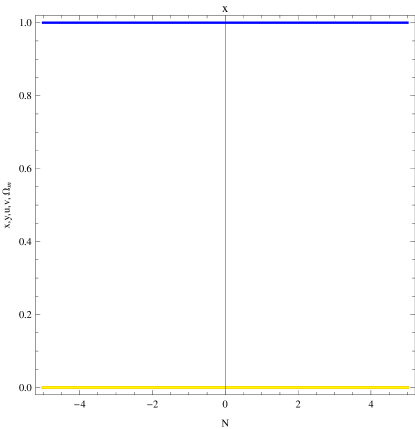
Figure 1: Plot of (1) variations of x (blue),y (green),u (orange),v (red),$\Omega_{m}$ (yellow) versus N near $P_{1}$, for $\gamma=1$ , $\delta=0.5$ and $\lambda=-0.5.$.The position corresponding N=0 is the fixed point under consideration.

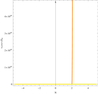
Figure 2: Plot of(2) variations of x (blue),y (green),u (orange),v (red),$\Omega_{m}$ (yellow) versus N near $P_{2}$, for $\gamma=1$ , $\delta=0.5$ and $\lambda=-0.5.$ The position corresponding N=0 is the fixed point under consideration.

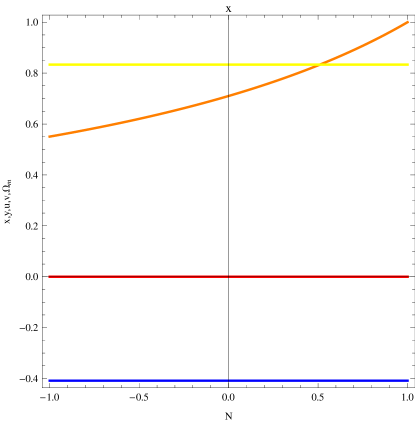
Figure 3: Plot of (3) variations of x (blue),y (green),u (orange),v (red),$\Omega_{m}$ (yellow) versus N near $P_{4}$, for $\gamma=4/3$ , $\delta=0.5$ and $\lambda=-0.5.$ The position corresponding N=0 is the fixed point under consideration.

If, ${\delta^{2}}{\leq}\frac{3}{2}$ and ${\delta^{2}}-\delta\lambda{\leq}-\frac{3}{2}$ (equality should occur in one of them) $P_{4}$ may admit 2 dimensional stable manifold corresponding the two negative eigenvalues with Eos of hessence is 1 and total Eos is $-1+\gamma(1-\frac{2{\delta^{2}}}{3})+\frac{4{\delta^{2}}}{3}$ and universe decelerates.Here, the plot figure $\mathbf{3}$ indicates that with a small increase of N the solution moves away from $P_{4}$.This is a unstable fixed point.

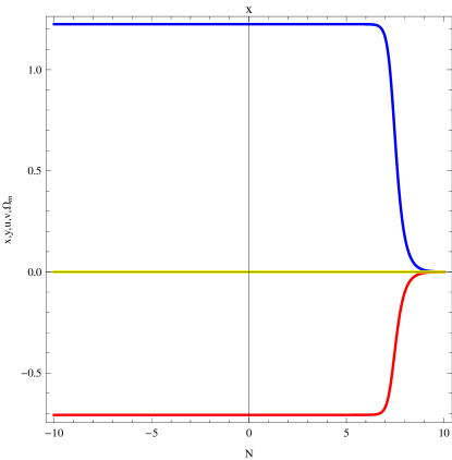
Figure 4: Plot of (4) variations of x (blue),y (green),u (orange),v (red),$\Omega_{m}$ (yellow) versus N near $P_{5}$,for $\gamma=1$ , $\delta=1$ and $\lambda=-0.5.$ The position corresponding N=0 is the fixed point under consideration.

Figure 5: Plot of (5) variations of x (blue),y (green),u (orange),v (red),$\Omega_{m}$ (yellow) versus N near $P_{6}$, for $\gamma=1$ , $\delta=1$ and $\lambda=-0.5.$ The position corresponding N=0 is the fixed point under consideration.

We note that for $P_{5}$ and $P_{6}$ if, $x\delta{\leq}-\sqrt{\frac{3}{2}}$ and $x\lambda{\leq}-\sqrt{6}$ (equality should occur in one of them) $P_{5}$ may admit 2 dimensional stable manifold corresponding the two negative eigenvalues and $P_{6}$ too may admit 2 dimensional stable manifold corresponding the two negative eigenvalues with Eos of hessence is 1 and total Eos is 1 and universe decelerates. The figure $\mathbf{4}$ indicates that the three of the variables (namely $x,v,$$\Omega_{m}$) are moving away from $P_{5}$ and intruding in a neighbourhood of N=10. This may denote the stable manifold corresponding the negative eigenvalues.However, this point gives the decelerated phase of the universe. Similar phenomena can be noted from figure $\mathbf{5}$.

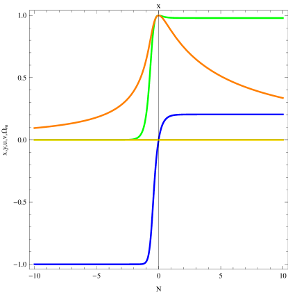
Figure 6: Plot of (6) variations of x (blue),y (green),u (orange),v (red),$\Omega_{m}$ (yellow) versus N near $P_{7}$,for $\gamma=0$ , $\delta=1$ and $\lambda=-0.5.$ The position corresponding N=0 is the fixed point under consideration.

Figure 7: Plot of (7) variations of x (blue),y (green),u (orange),v (red),$\Omega_{m}$ (yellow) versus N near $P_{8}$,for $\gamma=0$ , $\delta=1$ and $\lambda=-0.5.$ The position corresponding N=0 is the fixed point under consideration.

We note that if $\delta\lambda-{\lambda^{2}}{\leq}3$ both $P_{7}$ and $P_{8}$ are normally hyperbolic set of fixed points and as the rest three non-zero eigenvalues are negative they are stable. The set of fixed points has Eos of hessence is $-1$ and total Eos is also $-1$ and universe accelerates like ‘cosmological constant’. We note clearly from figures $\mathbf{6}$ and $\mathbf{7}$ that all lines from negative and positive values of N (i.e., from past and future) are converging towards N=0 (i.e., the set of fixed points).

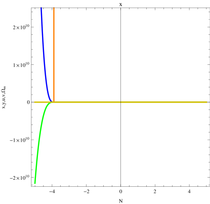
Figure 8: Plot of (8) variations of x (blue),y (green),u (orange),v (red),$\Omega_{m}$ (yellow) versus N near $P_{9}$,for $\gamma=1$ , $\delta=1$ and $\lambda=-0.5.$ The position corresponding N=0 is the fixed point under consideration.

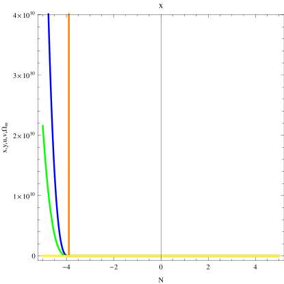
Figure 9: Plot of (9) variations of x (blue),y (green),u (orange),v (red),$\Omega_{m}$ (yellow) versus N near $P_{10}$,for $\gamma=1$ , $\delta=1$ and $\lambda=-0.5.$ The position corresponding N=0 is the fixed point under consideration.

We note that if ${\lambda^{2}}{\leq}6$ and ${\lambda^{2}}-\delta\lambda{\leq}3$ (equality should occur in one of them) $P_{9}$ and $P_{10}$ may admit 3 dimensional stable manifold corresponding the negative eigenvalues with Eos of hessence $-1+\frac{\lambda^{2}}{3}$ and total Eos also $-1+\frac{\lambda^{2}}{3}$, (i.e., both Eos are ‘quintessencelike’ if ${\lambda^{2}}<3$ or ‘dustlike’ if ${\lambda^{2}}=3$ ). The graphs in figure $\mathbf{8}$ and $\mathbf{9}$ also supports the fact corresponding the stable manifolds. In our choice of $\lambda=-0.5$, Eos of hessence and total Eos, both behaves like ‘quintessence’.

Figure 10: Plot of (10) variations of x (blue),y (green),u (orange),v (red),$\Omega_{m}$ (yellow) versus N near $P_{11}$,for $\gamma=1$ , $\delta=1$ and $\lambda=-0.5.$ The position corresponding N=0 is the fixed point under consideration.

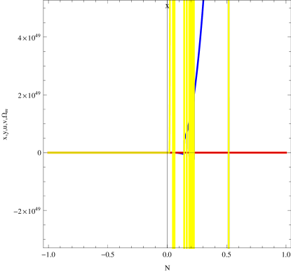
Figure 11: Plot of (11) variations of x (blue),y (green),u (orange),v (red),$\Omega_{m}$ (yellow) versus N near $P_{12}$,for $\gamma=1$ , $\delta=1$ and $\lambda=-0.5.$ The position corresponding N=0 is the fixed point under consideration.

We note that if ${a^{2}}+\frac{b^{2}}{2}{\leq}1,D{\leq}-\sqrt{\Delta}$ (equality should occur in one of them) $P_{11}$ and $P_{12}$ may admit 3 dimensional stable manifold corresponding the negative eigenvalues with Eos of hessence $\frac{-1+2{A^{2}}+{B^{2}}}{1-B}$ and total Eos $-1+{A^{2}}+{B^{2}}+(\gamma-2)B$. We see from figure $\mathbf{10}$ that the system is moving away from the fixed point $P_{11}$. Similar phenomena happens for fixed point $P_{12}$ as seen from figure $\mathbf{11}$.

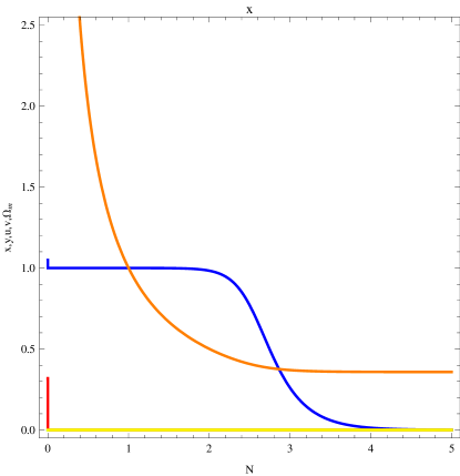
Figure 12: Plot of (12) variations of x (blue),y (green),u (orange),v (red),$\Omega_{m}$ (yellow) versus N near $P_{13}$,for $\gamma=1$ , $\delta=1$ and $\lambda=-0.5.$ The position corresponding N=0 is the fixed point under consideration.

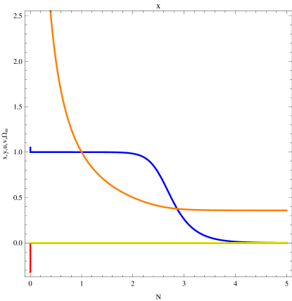
Figure 13: Plot of (13) variations of x (blue),y (green),u (orange),v (red),$\Omega_{m}$ (yellow) versus N near $P_{14}$,for $\gamma=1$ , $\delta=1$ and $\lambda=-0.5.$ The position corresponding N=0 is the fixed point under consideration.

We note that if $2\delta<\lambda<0$ or $0<\lambda<2\delta$, then $P_{13}$ and $P_{14}$ may admit 1 dimensional stable manifold corresponding the negative eigenvalues with Eos of hessence and total Eos being 1 and universe decelerates. The graphs figure $\mathbf{12}$ and figure $\mathbf{13}$ shows that the system is diverging from the fixed point $P_{13}$ and $P_{14}$. So, both the points are unstable in nature.

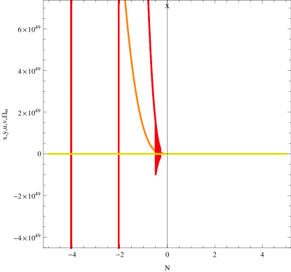
Figure 14: Plot of (14) variations of x (blue),y (green),u (orange),v (red),$\Omega_{m}$ (yellow) versus N near $P_{15}$,for $\gamma=1$ , $\delta=1/(4\sqrt{6})$ and $\lambda=-0.5.$ The position corresponding N=0 is the fixed point under consideration.

Figure 15: Plot of (15) variations of x (blue),y (green),u (orange),v (red),$\Omega_{m}$ (yellow) versus N near $P_{16}$,for $\gamma=1$ , $\delta=1/(4\sqrt{6})$ and $\lambda=-0.5.$ The position corresponding N=0 is the fixed point under consideration.

We note that if $x\delta{\leq}-\sqrt{\frac{3}{2}}$ and $x\lambda{\leq}-\sqrt{6}$ then $P_{15}$ and $P_{16}$ may admit 2 dimensional stable manifold corresponding the two negative eigenvalues with Eos of hessence and total Eos being 1 and universe decelerates. Here, we note that the solution set of the dynamical system moving rapidly from the fixed points $P_{15}$ and $P_{16}$ as clear from figures $\mathbf{14}$ and $\mathbf{15}$.The fixed points are unstable.

5 Cosmological Significance of the Fixed Points

In this section we discuss about the possible singularities that any dark energy model could have and compare the fixed points against recent dataset Planck 2015 data [27]. If the Eos $\omega{\leq}-1$ (i.e., the null energy condition $p+\rho{\geq}0$ is violated) and Big rip singularity happens within a finite time [20]. This singularity happens when at finite time $t{\rightarrow}t_{s}$, $a{\rightarrow}{\infty}$, $\rho{\rightarrow}{\infty}$ and $|p|{\rightarrow}{\infty}$.
We now analyse the stable fixed points to see if they can avoid (or, suffer) Big rip singularity. For the stable fixed points $P_{7}$ and $P_{8}$ or, we have $\dot{H}/{H^{2}}=0$ which gives $H=k$ (the integral constant), we get $a{\varpropto}{e^{kt}}$. Also, in these cases ${\omega_{total}}=-1$ which with energy conservation equation gives $\rho=constant$. Hence universe suffers no Big rip here. Fixed points $P_{7}$ and $P_{8}$ exist with physical parameter ${\Omega_{m}}=0$, ${\omega_{h}}=-1$, ${\omega_{total}}=-1$. The value of the parameters are well within the best fit of Planck 2015 data i.e., ${\Omega_{m}}=0.3089{\pm}0.0062$ from TT, TE, EE+low P+lensing+ext data, and Eos of dark energy $\omega={-1.019}^{+0.075}_{-0.080}$
Now, we consider the unstable fixed points. An unstable fixed point may describe the initial phase of universe, whereas a stable fixed point may be the end phase of the universe. For fixed points $P_{1}$, $P_{2}$ and $P_{3}$ exist with the physical parameter ${\Omega_{m}}=0$, ${\omega_{h}}=1$, ${\omega_{total}}=1$. Clearly, no Big rip occurs here.Here, the parameter ${\Omega_{m}}$ lies within the best fit of Planck 2015 data i.e., ${\Omega_{m}}=0.3089{\pm}0.0062$ from TT, TE, EE+low P+lensing+ext data. But,${\omega_{h}}$, ${\omega_{total}}$ defy the Eos of dark energy $\omega={-1.019}^{+0.075}_{-0.080}$.
Fixed point $P_{4}$ has values of physical parameters ${\Omega_{m}}=\frac{6-3\gamma+2\delta^{2}}{3}$, ${\omega_{h}}=1$, ${\omega_{total}}=-1+\gamma(1-\frac{2{\delta^{2}}}{3})+\frac{4{\delta^{2}}}{3}$. Here, ${\omega_{h}}$ and ${\omega_{total}}$ both are greater than -1, no Big rip occurs here too. A wide choices of $\gamma$ and $\delta$ can can fit $\Omega_{m}$ and ${\omega_{total}}$ within Planck 2015 data i.e., ${\Omega_{m}}=0.3089{\pm}0.0062$, but ${\omega_{h}}$, disobey the Eos of dark energy $\omega={-1.019}^{+0.075}_{-0.080}$.
Fixed points $P_{5}$ ,$P_{6}$ exist with physical parameters ${\Omega_{m}}=0$, ${\omega_{h}}=1$, ${\omega_{total}}=1$. We observe this solution are devoid of Big rip.Here,${\Omega_{m}}$ lies within the best fit of Planck 2015 data data. But,${\omega_{h}}$, ${\omega_{total}}$ defy the Eos of dark energy $\omega={-1.019}^{+0.075}_{-0.080}$.
Fixed points $P_{9},P_{10}$ admit physical parameters as ${\Omega_{m}}=0$, ${\omega_{h}}=-1+\frac{\lambda^{2}}{3}$, ${\omega_{total}}=-1+\frac{\lambda^{2}}{3}$ and so avoid Big rip.Also, $\Omega_{m}$ is within Planck 2015 data. Also, suitable choice of $\lambda$ fits ${\omega_{h}}$, ${\omega_{total}}$ within dataset.
Fixed points $P_{11}$ and $P_{12}$ have physical parameters ${\Omega_{m}}=B$, ${\omega_{h}}=\frac{-1+2{A^{2}}+{B^{2}}}{1-B}$, ${\omega_{total}}=-1+{A^{2}}+{B^{2}}+(\gamma-2)B$, where $A=-\sqrt{\frac{3}{2}}~{}\frac{\gamma}{\delta+\lambda}$ and $B=\frac{6+\lambda\sqrt{6}A-6{A^{2}}}{9}$. Here, we can adjust $A$ and $B$ to make ${\omega_{h}}$ and ${\omega_{total}}{\geq}-1$ to miss Big rip. Since, only, $0<\gamma{\leq}2$ but, $\delta$ can take arbitrary small value and $\lambda$ can have any real value, $A$ and hence, $B$ can be adjusted well within Planck ${\Omega_{m}}=0.3089{\pm}0.0062$ from TT, TE, EE+low P+lensing+ext data and Eos of dark energy $\omega={-1.019}^{+0.075}_{-0.080}$ data.
Fixed points $P_{13}$,$P_{14}$, $P_{15}$ and $P_{16}$ can avoid Big rip, as they bear physical parameters ${\Omega_{m}}=0$, ${\omega_{h}}=1$, ${\omega_{total}}=1$.Here, the parameter ${\Omega_{m}}$ lies within the best fit of Planck 2015 data i.e., ${\Omega_{m}}=0.3089{\pm}0.0062$ from TT, TE, EE+low P+lensing+ext data. But, ${\omega_{h}}$, ${\omega_{total}}$ totally defy the Eos of dark energy $\omega={-1.019}^{+0.075}_{-0.080}$.

6 Concluding Remarks

In this paper we have performed a dynamical system study of an unique scalar field hessence coupling with dark matter in an alternate theory of gravity, namely $f(T)$ gravity. The system is unconventional, complex but quite interesting. The model is chosen to explore one of the various possibilities about the fate of the universe. The sole purpose is to explain the current acceleration of universe. An unstable fixed point may describe the initial phase of universe, whereas a stable fixed point may be the end of the universe. We have chosen exponential form of potential of the form $V={V_{0}}{e^{\lambda\phi}}$ (where $V_{0}$ and $\lambda$ are real constant and $\phi$ is the hessence field) for simplicity. The interaction term $C$ is chosen to solve the so called ‘cosmological constant’ problem in tune with second law of thermodynamics and is quite arbitrary (only $C$ should remain positive), since $C=\delta\dot{\phi}\rho_{m}$, where $\delta$ is a real constant of small magnitude, which may be chosen as positive or negative, such that $C$ remains positive. Also, $\dot{\phi}$ may be positive or negative according the hessence field $\phi$. The resulting non linear dynamical system gives sixteen possible fixed points. Among them $P_{7}$ and $P_{8}$ are stable set of normally hyperbolic fixed points, which resembles like ‘cosmological constant’, so it explain the current phase of acceleration of universe. But, interestingly it does not show ‘hessence like’ nature. Among the other fixed points the initial phases of evolution may begin. However, the complexity of the system is main obstacle for a precise explanation. Anyway, in future work, we may try some other possible alternative.

Conflict of Interest: The authors declare that there is no conflict of interest regarding the publication of this paper.

Acknowledgement: One of the authors (UD) is thankful to IUCAA, Pune, India for warm hospitality where part of the work was carried out.

References

- [1] A.G.Riess et al. [Suparnova Search Team Collaboration],Astrophysics J.607 665,(2004),astro-ph/0402512
- [2] R.A.Knopp et al. [Suparnova Cosmology Project Collaboration],Astrophysics J.598 102,(2003),astro-ph/0309368
- [3] P.Astier et al. [SNLS Collaboration],Astron. Astrophysics 447 31,(2006),astro-ph/0510447
- [4] J.D.Neill et al. [SNLS Collaboration],astro-ph/0605148
- [5] C.L.Benett et al. [WMAP Collaboration],Astrophysics J. Suppl. 148 1, (2003),astro-ph/0302207
- [6] D.N.Spergell et al. [WMAP Collaboration],Astrophysics J. Suppl. 148 175, (2003),astro-ph/0302209
- [7] D.N.Spergell et al. [WMAP Collaboration],astro-ph/0603449
- [8] L.Page et al. [WMAP Collaboration],astro-ph/0603450
- [9] G.Hinshaw et al. [WMAP Collaboration],astro-ph/0603451
- [10] N.Jarosik et al. [WMAP Collaboration],astro-ph/0603452
- [11] E. Komatsu et al. [WMAP Collaboration],Astrophysics J. Suppl. 192 18, (2011).
- [12] M.Tegmark et al. [SDSS Collaboration],Phys. Rev. D. 69 103501, (2004),astro-ph/0310723
- [13] M.Tegmark et al. [SDSS Collaboration],Astrophysics J. 606 702, (2004),astro-ph/0310725
- [14] U.Seljak et al.,Phys. Rev. D. 71 103515, (2005),astro-ph/0407372
- [15] J.K.Adelman-McCarthy et al. [SDSS Collaboration],Astrophysics J. Suppl. 162 38, (2006),astro-ph/0507711
- [16] K.Abazajian et al.[SDSS Collaboration],astro-ph/0410239,astro-ph/0403325,astro-ph/0305492
- [17] M.Tegmark et al. [SDSS Collaboration],astro-ph/0608632
- [18] S.W.Allen,R.W.Schmidt,H.Ebeling,A.C.Fabian and L Van Speybroeck Mon. Not. Roy. Astron. Soc. 353 457, (2004),astro-ph/0405340
- [19] A.G.Riess et al. [Suparnova Search Team Collaboration],astro-ph/0611572
- [20] E.J.Copeland, M. Sami, S. Tsuzikawa, Int. Journal Of Modern Physics D11, 1753-1935 (2006).
- [21] S.Weinberg, Rev. Mod. Phys. 61,1 (1989).
- [22] P.J.E.Peebles, B.Ratra, Rev. Mod. Phys. 75,559 (2003).
- [23] T, Padmanabhan, Curr. Sci. 88,1057 (2005).
- [24] J.Martin, M.Yamaguchi,Phys.Rev.D77, 123508 (2008).
- [25] L,P.Chimento, R.Lazkoz, I.Sendra, Gen. Rel. Grav.,DOI:10.1007/s10714-009-0901z (2009).
- [26] P.A.R.Ade et al.,Planck 2013 results XVI.Cosmological Parameters,Astron. Astrophys,571:A16,(2014).
- [27] P.A.R.Ade et al.,arXiv 1502:01589 [astro-ph].
- [28] A. Albrecht and P. J. Steinhardt,Phys. Rev. Lett.48,(1982) 1220 [INSPIRE];A complete description of inflationary models can be found in the book by A. Linde, Particle Physicss and Inflationary Cosmology, Gordon and Breach, New York U.S.A. (1990).
- [29] A. H. Guth, Phys. Rev. D23, (1981) 347.
- [30] A. Berera, I. J. Moss, R. O. Ramos, Rep. Prog. Phys.70, (2009) 026901.
- [31] A. Berera, L. Z. Fang, Phys. Rev. Lett.74, (1995) 1912.
- [32] A. Berera, Phys. Rev. Lett.75, (1995) 3218; Phys. Rev. D55, (1997) 3346.
- [33] P.Steinhardt,Critical problems in Physics,(Princeton University Press)Princeton,NJ (1997).
- [34] I.Zlatev,L.M.Wang,P.J.Steinhardt,Phys.Rev.Lett.82,896(1999).
- [35] S.M.Carrol,Phys.Rev.Lett.81, 3067 (1998).
- [36] U.Alam,V.Sahni,T.D.Saini,A.A.Starobinsky,Mon.Not.R.Ast.Soc 354,275(2004).
- [37] R.R.Caldwell,Phys.Lett.B 545,23(2002).
- [38] R.R.Caldwell,M.Kamionkowski,N.N.Weinberg,Phys.Rev.Lett.91,071301(2003).
- [39] R.J.Scherrer,Phys.Rev.D 71,063519 (2005).
- [40] L.P.Chimento,M.I.Forte,R.Lazcoz,M.G.Richarte,Phys.Rev.D 79,0435002 (2009).
- [41] B.Feng,X.L.Wang,X.M.Zhang,Phys.Lett.B 607,35 (2005).
- [42] L.A.Boyle,R.R.Caldwell,M.Kamionkowski,Phys.Lett.B 545,17(2002).
- [43] S.Kasuya,Phys.Lett.B 515,121 (2001).
- [44] H. Wei,R-G Cai,D-F Zeng,Class. Quant. Grav.22, (2005) 3189;
- [45] H. Wei,R-G Cai,Phys. Rev. D 72, (2005) 123507.
- [46] H. Wei,R-G Cai,Phys. Rev. D 72, (2005) 123507;
- [47] M. Alimohammadi,H.M. Sadjadi,Phys. Rev. D 73,(2005) 083527;
- [48] H. Wei,N. Tang and S. N. Zhang,Phys. Rev. D 75,(2007) 043009.
- [49] S.Capozziello,Int.J.Mod.Phys,D 11,(2002).
- [50] S.Nojiri,S.D.Odintsov,Phys.Rev.D 68,(2003) 123512.
- [51] S.M.Carroll,V.Duvvuri,M.Trodden,M.S.Turner,Phys.Rev.D70,(2004) 043528.
- [52] A.Einstein,Sitzungsber.Preuss.Akad.Wiss.Phys.Math.KI 217,(1928);ibid401,(1930).
- [53] A.Einstein,Math.Annal102,685 (1930).
- [54] K.Hayashi,T.Shirafuji,Phys.Rev.D19,3524 (1979);[Addendum-ibid24,3312(1982)].
- [55] R.Aldrovandi,J.G.Pereira,Teleparallel Gravity:An Introduction,Springer,Dordrecht (2012).
- [56] M.P.Gaugh,arXiv 1607:00330.
- [57] A.Behboodi,S.Akshabi,K.Nozari, Phys. Lett. B 718, 30 (2012); arXiv 1205:4570[gr-qc].
- [58] E.Dil,E.Colay,Adv.H.E.P.608252 (2015).
- [59] R.Lazcoz,G.Leon,I.Quiros,arXiv 0701353:[astro-ph].
- [60] H. Wei, S. N. Zhang,arXiv 0705:4002:[gr-qc].
- [61] S. K. Biswas and S. Chakraborty, Int.J.Mod.Phys. D 24, 1550046 (2015).
- [62] E.E.Flanagan,E.Rosenthal,Phys.Rev.D19,124016 (2007).
- [63] J.Garecki,arXiv 1010:2654[gr-qc].
- [64] G.R.Bengochea,R.Ferraro,Phys.Rev.D79,124019 (2009).
- [65] E.V.Linder,Phys.Rev.D81,127301 (2010) [Erratum-ibidD82,109902 (2010)].
- [66] P.Wu,H.Yu, Phys.Lett.B,693,415 (2010).
- [67] P.Wu,H.Yu,Eur.Phys.J,C,71,1552 (2011).
- [68] M.R.Setare,M.J.S.Houndjo,arXiv 1203:1315v1 [gr-qc].
- [69] M.H.Daouda,M.E.Rodrigues,M.J.S.Houndjo,Eur.Phys.J,C,72,1893 (2012).
- [70] V.F.Cardone,N.Radicella,S.Camera,Phys.Rev.D,85,124007 (2012).
- [71] S.Camera,V.F.Cardone,N.Radicella,Phys.Rev.D,89,083520 (2014).
- [72] K.Bamba,M.Jamil,D.Momeni.R.Myrzakulov,arXiv 1202:6114v1[physics, gen-ph].
- [73] G.Dvali,G.Gabadadze,M.Porrati,Phys.Lett.B,485,208 (2000).
- [74] C.Deffayet,G.Dvali,G.Gabadadze,Phys.Rev.D 65,044023 (2002).
- [75] K.Nozari,N.Behrouz, Physics of the Dark Universe, 13, 92 (2016); arXiv 1605:06028 [gr-qc].
- [76] N.Mahata,S.Chakraborty, arXiv 1512:07017 [gr-qc].
- [77] J. Wainwright, G.F.R.Ellis edited, Dynamical Systems in Cosmology,Cambridge University Press,Cambridge (1997).
- [78] B.Aulbach, Continuous and Discrete Dynamics near Manifolds of Equilibria,Lecture Notes in Mathtematics [Chapter 4] Springer-Verlag (1984).