Mesoscopic Modeling of Random Walk and Reactions in Crowded Media

Abstract

We develop a mesoscopic modeling framework for diffusion in a crowded environment, particularly targeting applications in the modeling of living cells. Through homogenization techniques we effectively coarse-grain a detailed microscopic description into a previously developed internal state diffusive framework. The observables in the mesoscopic model correspond to solutions of macroscopic partial differential equations driven by stochastically varying diffusion fields in space and time. Analytical solutions and numerical experiments illustrate the framework.

Keywords: subdiffusion, crowding, internal states, reaction-diffusion system.

1 Introduction

Living cells are controlled by a complicated network of reaction-diffusion events. An example is exogenous signals triggering the cell’s response by reacting with the proteins present in the cell or binding to the DNA to initiate transcription of certain genes. An important task in computational systems biology is to study these processes as accurately as possible inside the complicated cell geometry. We specifically target two special features in a model of the biochemical processes in living cells in this article: the high percentage of occupied volume in the cytoplasm and the intrinsic noise.

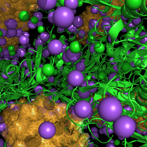
Figure 1.1: A snapshot from a molecular dynamics simulation: the interior of an E. coli is a highly crowded environment. Picture courtesy of David van der Spoel, Uppsala university.

It is estimated that up to 40% of the available space in the cytoplasm is occupied by macromolecules [1, 2] and these have been shown to alter the dynamics of the reaction network [3], see also Figure 1.1. Due to the multiple steric repulsions between the tracer molecules and the crowders, diffusion is slowed down. This macromolecular crowding effect plays an even more important role on the cell membrane [4], where actin filaments create barriers for the motion of membrane bound proteins [5, 6, 7].

New imaging techniques [8] have shown that the slowdown happens gradually over time. The tracers initially diffuse freely without encountering the crowding macromolecules. Then they start colliding with the crowders and go through an anomalous phase of diffusion where their movement is constantly slowed down and their mean square displacement (MSD) therefore grows sublinearly with time [9, 10, 11]. On a long time scale they can be observed to be diffusing normally again, but at a reduced diffusion constant compared to the tracer in a dilute medium. This change in diffusivity is a hydrodynamic consequence of the highly crowded space inside cells. Moreover, the crowders also exhibit a thermodynamic effect on the chemical reactions [12], which can be both impeded (due to the longer time until collision) or facilitated (due to the smaller effective reaction volume). In this paper, we will only investigate inert crowders and their effect due to steric repulsion with the reacting molecules. More complicated interactions such as transient binding or interaction potentials further impact the reaction-diffusion dynamics in a crowded environment [13, 14, 15, 16], but lie outside the scope of this study.

The second feature we incorporate in our modeling framework is stochasticity. Although the cytosol is densely packed with molecules, the individual species is often present at low copy numbers. A deterministic macroscopic model describing the mean value of the concentrations of the chemical species is therefore not applicable and stochastic models remain as the computationally feasible alternative [17, 18, 19, 20, 21]. On a mesoscopic or on-lattice level of modeling, the domain is partitioned into voxels and diffusion is modeled as a random jump process of the molecules between the voxels. Inside each voxel, space is not resolved further and the molecules are assumed to be well mixed and react randomly with other molecules located within the same voxel. The time evolution of this system is described by the reaction-diffusion master equation [22]. We sample trajectories of the system using stochastic simulation techniques as popularized by Gillespie [23], originally developed for well stirred problems without spatial dependence. Discretizations of spatial domains were first considered in [24, 25, 26] and later improved to allow for unstructured meshes in [27, 28]. Overviews of deterministic, macroscopic and stochastic, mesoscopic and microscopic levels of modeling of biochemical networks are found in e.g. [29, 30, 31].

There have been several models combining the macromolecular crowding effects and the stochastic mesoscopic level. In [32] the most highly crowded voxels are defined as full and are made inaccessible for the tracer molecules in order to model crowding. A more gradual approach is to define the number of possible molecules per voxel and then rescale the propensity to jump into this voxel by how many spots are already occupied by other molecules [33, 34, 35]. But by averaging the effect of the crowders over the whole voxel, the transient anomalous phase is not captured and we only observe the long time slower diffusion. To resolve the short-time microscopic information the positions of stationary obstacles were homogenized (or coarse-grained, upscaled) to mesoscopic jump rates in [36]. Here, the crowders can have arbitrary shape, but the diffusing tracers are understood to be circular in two space dimensions (2D) and spherical in three dimensions (3D).

In Brownian dynamics each individual molecule is tracked in a lattice-free (or off-lattice) microscopic model. Here, all molecules are spherical, move in Brownian motion, and react with a certain probability when they touch each other [37, 38]. Crowding is automatically incorporated in the model by the excluded volume of the stationary or moving crowders. A stochastic, microscopic simulation is in general more accurate than a mesoscopic simulation but also much more computationally expensive. Microscopic simulation of crowding and diffusion at the particle level is proposed in [39] and is evaluated in [40, 11]. In [41] off-grid microscopic simulations are compared to grid based microscopic cellular automata simulations and the grid artifacts are quantified.

On the deterministic, macroscopic level, anomalous diffusion of the concentrations due to crowding can be modeled by fractional partial differential equations (FPDEs) [42, 10, 43]. Internal states are introduced in [44] on the mesoscopic level to model anomalous diffusion and in [45] for reactions. The internal state of a molecule changes with a certain probability and determines the molecule’s diffusion speed. The intensities for these changes are given by the macroscopic FPDE for the observed variables in [45, 44]. Memory effects are included without sacrificing the Markov property using these internal states. Three physical interpretations of these internal states are that the molecule is in different geometrical conformations, has different methylation or phosphorylation, or resides in differently crowded environments, which are all affecting the diffusion speed and reaction propensities. Hidden states are also introduced in [46] to explain data from single cell experiments.

In this paper, we will combine the internal states model derived in [45] with the multiscale approach in [36] to efficiently model diffusion of tracer particles among stationary or moving crowder obstacles. The method

1. is considerably faster than Brownian dynamics,

2. allows more versatile modeling than mesoscopic methods where a limited number of molecules can occupy a lattice node,

3. defines a random diffusion field for a macroscopic equation expressed in observables.

We first coarse-grain the microscale to the mesoscale by determining statistics for the variation in the diffusion coefficient with the homogenization method in [36]. The parameters of the internal states model in [45] can subsequently be deduced from these data. Our mesoscopic method for crowding is less heuristic than other methods and can be defined by experimental data, e.g., from [46]. The mesoscale equations are coarse-grained to the macroscale analytically resulting in PDEs for the observables.

In the next section we first present the two mesoscopic models from [45] and [36] in more detail. We couple the statistics from the microlevel to the parameters in the internal state model in Section 3. The distributions of the molecules in certain chemical systems with internal states and diffusion are multinomial as shown by the analysis in Section 4. In Section 5, we test the resulting coarse-grained model in examples in 2D and 3D and a summarizing discussion is found in the final section.

2 Two mesoscopic models

The effect of static crowding molecules is coarse-grained from the microscopic to the mesoscopic level of approximation according to [36]. Then a discretized mesoscopic model built from an internal states approximation is reviewed following [45, 44].

2.1 Microscopic to mesosocopic model via first exit times

Single tracer molecules move on the microscopic scale by Brownian motion in a domain $\omega_{\ast}$ with obstacles. The moving molecules are assumed to be circular in 2D and spherical in 3D with radius $r$. The crowder obstacles are stationary in space and chemically inert, such that the boundary condition for the moving molecule is reflective at the surface of the crowding objects, which are represented explicitly as holes in $\omega_{\ast}$. The volume of the interior of the cell is denoted by $\Omega$ and $\omega_{\ast}$ is a subvolume of $\Omega$, $\omega_{\ast}\subset\Omega$. The subvolumes $\omega_{\ast}$ are occupied by crowders such that the free space remaining for the moving molecule is $\omega$ and $\omega\subseteq\omega_{\ast}$, see Figure 2.1(a) and (b).

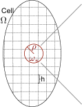
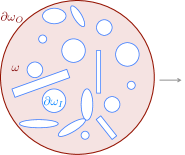
Figure 2.1: (a) The cell volume $\Omega$ discretized by a grid with size $h$ giving rise to the non-perforated subvolumes $\omega_{\ast}$. (b) The circular, perforated domain $\omega$ (pink) of radius $\rho$ where the cut-outs represent the obstacles, and the outer $\partial\omega_{O}$ and inner $\partial\omega_{I}$ boundaries. (c) Solution to (2.1) on $\omega$ with crowders represented as holes with reflective boundary conditions and with high values of $E(\mathbf{x})$ in red and low values in blue. (d) The excluded volume consists of the volume occupied by the crowding molecule enlarged by the radius $r$ of the diffusing tracer molecule.

Let $\gamma_{0}$ be the diffusion coefficient for the Brownian motion. In [36] we presented a multiscale approach to compute the effective diffusion rate $\gamma$ in the crowded environment $\omega_{\ast}$ using the mean value of the first exit time $E(\mathbf{x})$, see [47], from $\omega$ fulfilling

$$\gamma_{0}\Delta E(\mathbf{x}) =-1, \mathbf{x} \in\omega,$$ (2.1)

$$E(\mathbf{x}) =0, \mathbf{x} \in\partial\omega_{O},$$ (2.2)

$$\mathbf{n}\cdot\nabla E(\mathbf{x}) =0, \mathbf{x} \in\partial\omega_{I}.$$ (2.3)

The starting position of the diffusing molecule is $\mathbf{x}\in\omega$, $\partial\omega_{O}$ is the outer boundary of $\omega$ shared with $\omega_{\ast}$ and $\partial\omega_{I}$ is the inner boundary of the obstacles with normal $\mathbf{n}$, see Figure 2.1(b). Since (2.1) describes the expected exit time of a moving point particle, the cut-outs in the perforated domain are enlarged to account for the radius $r$ of the tracer, see Figure 2.1(d).

Equation (2.1) and boundary condition (2.2) also hold on the non-perforated domain $\omega_{\ast}$ without the boundary condition on $\partial\omega_{I}$ and resulting in the solution $E_{\ast}(\mathbf{x})$. Since the mean first exit time in (2.1) is inversely proportional to the diffusion coefficient it can be used to compute the effective diffusion rate $\gamma$ in the crowded domain $\omega_{\ast}$ according to

$$\gamma=\gamma_{0}\frac{E_{\ast}(\mathbf{x})}{E(\mathbf{x})}.$$ (2.4)

In this way, all the details in $\omega$ are avoided and an effective (or homogenized, upscaled, coarse-grained) diffusion coefficient $\gamma$ in $\omega_{\ast}$ is determined. The domain $\omega_{\ast}$ and point $\mathbf{x}$ are arbitrary but if $\omega_{\ast}$ is circular ($d=2$) or spherical ($d=3$) with radius $\rho$ then (see [47])

$$E_{\ast}(\mathbf{x})=\frac{1}{\gamma_{0}}\frac{\rho^{2}-\|\mathbf{x}\|^{2}_{2}}{2d}.$$ (2.5)

The effective diffusion rate $\gamma$ depends on the percentage of excluded volume $\phi\in[0,1]$. If $\phi=0$ then $E_{\ast}(\mathbf{x})=E(\mathbf{x})$ and $\gamma=\gamma_{0}$ in (2.4) and if $\phi\rightarrow 1$ then there is no space left for molecular motion, $E(\mathbf{x})\rightarrow\infty$, and $\gamma\rightarrow 0$. Depending on the shape of the obstacles and the size of the moving molecule $r$, $\gamma$ can be $0$ for a small $\phi<1$.

This approach is universal in the way that the stationary crowding molecules can have any shape. New $\gamma$ values for other shapes are determined in [36]. If the crowders are spherical with radius $R$, the radii have to satisfy $r,R\ll\rho$ for the upscaling to be accurate and not too sensitive to the particular distribution of the obstacles. The typical size of a moving or crowding molecule is 4-20 nm (globular protein-ribosome). Then a possible $\rho$ is $\rho\sim 50$ nm, which is sufficiently small to discretize a prokaryote E. coli of size $1-3\,\mu{\rm m}$ or an eukaryote cell which is about ten times larger.

2.2 The internal states model

The mesoscopic model for diffusion and chemical reactions is extended such that each molecule can adopt several internal states that may be unobservable. These extra internal states are used to model subdiffusion in [45, 44] and will be used here to represent crowding with moving obstacles.

2.2.1 The spatial internal states model

Let $u(\mathbf{x},t,\xi)$ be the concentration of a molecular species at $\mathbf{x}\in\Omega$ at time $t\geq 0$ in a continuous internal state $\xi\in\Xi=[0,\xi_{\max}]\subset\mathbb{R}_{+}$. The rate of change from internal state $\eta$ to state $\xi$ is $A(\xi,\eta)$. At the boundary $\partial\Omega$ of $\Omega$ the molecules are reflected and the scalar diffusion $\gamma(\xi)$ is allowed to depend on the internal state. Then $u$ satisfies, for $t>0$,

$$\begin{array}[]{rl}u_{t}(\mathbf{x},t,\xi)&=\nabla\cdot\left(\gamma(\xi)\nabla u(\mathbf{x},t,\xi)\right)+\int_{\Xi}A(\xi,\eta)u(\mathbf{x},t,\eta)\,d\eta,\quad\mathbf{x}\in\Omega,\;\xi\in\Xi,\\ \mathbf{n}\cdot\nabla u&=0,\quad\mathbf{x}\in\partial\Omega,\;\xi\in\Xi.\end{array}$$ (2.6)

The total amount of the species $\int_{\Omega}\int_{\Xi}u(\mathbf{x},t,\xi)\,d\xi\,d\mathbf{x}$ should remain constant for mass conservation. By integrating (2.6) over $\Xi$ and $\Omega$ using the boundary condition on $\partial\Omega$, we obtain the time derivative

$$\begin{array}[]{lcl}\displaystyle{\partial_{t}\int_{\Xi}\int_{\Omega}u(\mathbf{x},t,\xi)\,d\xi\,d\mathbf{x}}\\ =\displaystyle{\int_{\Xi}\int_{\Omega}\nabla\cdot\left(\gamma(\xi)\nabla u(\mathbf{x},t,\xi)\right)\,d\mathbf{x}\,d\xi}\displaystyle{+\int_{\Xi}\int_{\Omega}\int_{\Xi}A(\xi,\eta)u(\mathbf{x},t,\eta)\,d\eta\,d\mathbf{x}\,d\xi}\\ =\displaystyle{\int_{\Xi}\gamma(\xi)\int_{\partial\Omega}\mathbf{n}\cdot\nabla u(\mathbf{x},t,\xi)\,ds\,d\xi}\displaystyle{+\int_{\Omega}\int_{\Xi}u(\mathbf{x},t,\eta)\int_{\Xi}A(\xi,\eta)\,d\xi\,d\eta\,d\mathbf{x}}\\ =\displaystyle{\int_{\Omega}\int_{\Xi}u(\mathbf{x},t,\eta)\int_{\Xi}A(\xi,\eta)\,d\xi\,d\eta\,d\mathbf{x}}.\end{array}$$ (2.7)

The time derivative of the total amount must vanish for all $u$. Thus, a sufficient condition on $A$ for this to hold is

$$\int_{\Xi}A(\xi,\eta)\,d\xi=0.$$ (2.8)

The observable $U(\mathbf{x},t)$ denotes the concentration of the molecule independent of its internal state and is defined by

$$U(\mathbf{x},t)=\int_{\Xi}u(\mathbf{x},t,\xi)\,d\xi.$$ (2.9)

If $A$ is chosen as in (2.8) then by (2.6), $U$ in (2.9) satisfies

$$U_{t}(\mathbf{x},t)=\nabla\cdot\int_{\Xi}\gamma(\xi)\nabla u(\mathbf{x},t,\xi)\,d\xi.$$ (2.10)

There is an ordinary diffusion equation for $U$ only if $\gamma$ is independent of $\xi$. With a diffusion tensor $\tilde{\gamma}_{i}(\mathbf{x},t),\;i=1,\ldots,d,$ such that

$$\tilde{\gamma}_{i}(\mathbf{x},t)=\int_{\Xi}\gamma(\xi)\partial_{x_{i}}u(\mathbf{x},t,\xi)\,d\xi/\partial_{x_{i}}\int_{\Xi}u(\mathbf{x},t,\xi)\,d\xi,$$

(2.10) can be written

$$U_{t}=\nabla\cdot\left(\tilde{\boldsymbol{\gamma}}(\mathbf{x},t)\nabla U\right),$$ (2.11)

but in general $\tilde{\boldsymbol{\gamma}}$ is not known explicitly.

A particular choice of $A$ is

$$A(\xi,\eta)=(\mu(\xi)-\delta(\xi-\eta))T(\eta)$$ (2.12)

with the Dirac measure $\delta$. Then (2.8) is fulfilled if $\mu$ is scaled such that

$$\int_{\Xi}\mu(\xi)\,d\xi=1.$$ (2.13)

In order to find the steady state solution of (2.6), we set tentatively

$$u_{\infty}(\xi)=\mu(\xi)/T(\xi).$$ (2.14)

Clearly,

$$\int_{\Xi}A(\xi,\eta)u_{\infty}(\eta)\,d\eta=0,$$ (2.15)

and $u_{\infty}$ is indeed a steady state solution of (2.6). A natural convention is to let $\mu(\xi)\geq 0$ and $T(\xi)>0$ for $u_{\infty}$ to be a non-negative concentration.

2.2.2 Discretization in space and internal states

Let $\Omega$ be discretized by a triangular (2D) or tetrahedral (3D) primal mesh with nodes at $\mathbf{x}_{i},\,i=1,\ldots,J$. The dual mesh consists of voxels $\mathcal{V}_{i},\,i=1,\ldots,J$, as in [28]. Each node $\mathbf{x}_{i}$ is associated with one voxel $\mathcal{V}_{i}$. The solution $u$ of (2.6) is approximated by the finite element method using linear basis functions $\varphi_{i}(\mathbf{x})$ satisfying $\varphi_{i}(\mathbf{x}_{i})=1$ and $\varphi_{i}(\mathbf{x}_{j})=0,\,j\neq i$. The internal state space $\Xi$ is partitioned into $K$ intervals $\mathcal{I}_{k}=[\xi_{k-1},\xi_{k}],\,k=1,\ldots,K,$ of length $\Delta\xi=\xi_{\max}/K$. In each interval $k$ there is a basis function $\psi_{k}$ such that $\psi_{k}(\xi)=1/\sqrt{\Delta\xi},\,\xi\in\mathcal{I}_{k}$, and $\psi_{k}(\xi)=0$ otherwise. Then $u_{h}$ approximating $u$ is

$$u_{h}(\mathbf{x},t,\xi)=\sum_{j=1}^{J}\sum_{l=1}^{K}u_{jl}(t)\varphi_{j}(\mathbf{x})\psi_{l}(\xi).$$ (2.16)

Insert $u_{h}$ into (2.6), multiply by a test function $\varphi_{i}(\mathbf{x})\psi_{k}(\xi)$ in a tensor product finite element space and integrate over $\Omega\times\Xi$ to derive an equation for the evolution of $u_{jl}$. If $\xi$ in (2.6) is interpreted as a random variable determining the diffusion, then (2.16) is the approximation suitable for a stochastic Galerkin method to solve (2.6) [48].

Let $E_{\alpha}$ be a triangular element in 2D or a tetrahedral element in 3D with area or volume $|E_{\alpha}|$ and $\mathcal{T}_{ij}$ the set of triangles or tetrahedra with a common edge $ij$ between nodes $i$ and $j$. The Kronecker delta is denoted by $\delta_{ij}$. An element in the stiffness tensor $S$ is then

$$\begin{array}[]{rl}S_{ijkl}&=\displaystyle{-\sum_{E_{\alpha}\in\mathcal{T}_{ij}}\int_{E_{\alpha}}\nabla\varphi_{i}^{T}|_{E_{\alpha}}\nabla\varphi_{j}|_{E_{\alpha}}\,d\mathbf{x}\int_{\Xi}\gamma(\xi)\psi_{k}(\xi)\psi_{l}(\xi)\,d\xi}\\ &=\displaystyle{-\sum_{E_{\alpha}\in\mathcal{T}_{ij}}\nabla\varphi_{i}^{T}|_{E_{\alpha}}\nabla\varphi_{j}|_{E_{\alpha}}|E_{\alpha}|\gamma_{k}\delta_{kl}=\gamma_{k}S_{ij}\delta_{kl},}\end{array}$$ (2.17)

where $\gamma_{k}$ is the average of $\gamma(\xi)$ in $\mathcal{I}_{k}$. In the diagonal element with $i=j$, the integration domain in $\mathbf{x}$ is over all $E_{\alpha}$ with a corner at $\mathbf{x}_{i}$. Choose $\gamma_{k}$ to be $\gamma_{0}T(k)$ and let $\mathbf{T}$ be the matrix with $T(k)$ in the diagonal. Hence, with a stiffness matrix $\mathbf{S}$ the stiffness tensor in (2.17) can be written

$$S=\gamma_{0}\mathbf{S}\otimes\mathbf{T},$$ (2.18)

where $\otimes$ denotes the Kronecker product.

The mass tensor $\tilde{M}$ is defined by

$$\tilde{M}_{ijkl}=\sum_{E_{\alpha}\in\mathcal{T}_{ij}}\int_{E_{\alpha}}\varphi_{i}(\mathbf{x})\varphi_{j}(\mathbf{x})\,d\mathbf{x}\,\int_{\Xi}\psi_{k}(\xi)\psi_{l}(\xi)\,d\xi=\tilde{M}_{ij}\delta_{kl}.$$ (2.19)

The first part of $\tilde{\mathbf{M}}$ depends on the geometry and is lumped and replaced by a diagonal matrix $\mathbf{M}$ such that

$$M_{ij}=M_{i}\delta_{ij},\quad M_{i}=\sum_{l=1}^{J}\tilde{M}_{il}.$$ (2.20)

Then by (2.19)

$$\tilde{M}_{ijkl}=M_{i}\delta_{ij}\delta_{kl}.$$ (2.21)

An element in the tensor discretizing the operator $A$ for change of internal state is

$$\begin{array}[]{ll}A_{ijkl}&=\displaystyle{-\sum_{E_{\alpha}\in\mathcal{T}_{ij}}\int_{E_{\alpha}}\varphi_{i}(\mathbf{x})\varphi_{j}(\mathbf{x})\,d\mathbf{x}\int_{\Xi}\int_{\Xi}A(\xi,\eta)\psi_{k}(\xi)\psi_{l}(\eta)\,d\xi\,d\eta}\\ &=\displaystyle{\kappa_{0}\tilde{M}_{ij}A_{kl}},\end{array}$$ (2.22)

where $A_{kl}$ is an element in the matrix $\mathbf{A}$ and $\kappa_{0}$ is a freely choosable scaling of $\mathbf{A}$ that denotes how fast the molecules change their internal state. Thus, $A$ can be written as $A=\kappa_{0}\mathbf{M}\otimes\mathbf{A}$ after mass lumping of $\tilde{M}$.

Let $\mathbf{e}_{J}$ be defined by $\mathbf{e}^{T}_{J}=(1,1,\ldots,1)\in\mathbb{R}^{J}$ and let $\mu(\xi)$ be a piecewise constant function such that $\mu(\xi)=\sum_{k=1}^{K}\mu_{k}\psi_{k}(\xi)$. Then the matrix-vector forms of the condition in (2.8), the special choice of $A$ in (2.12), the scaling of the components of $\boldsymbol{\mu}$ in (2.13), and the null vector $\mathbf{u}_{i\infty}$ of $\mathbf{A}$ in (2.14) are

$$\begin{array}[]{ll}\mathbf{e}_{K}^{T}\mathbf{A}=\mathbf{0},\;\mathbf{A}=(\boldsymbol{\mu}\mathbf{e}_{K}^{T}-\mathbf{I}_{K})\mathbf{T},\;\mathbf{e}_{K}^{T}\boldsymbol{\mu}=1,\\ \mathbf{u}_{i\infty}=\mathbf{T}^{-1}\boldsymbol{\mu}\Longrightarrow\mathbf{A}\mathbf{u}_{i\infty}=\mathbf{0},\end{array}$$ (2.23)

where $\mathbf{I}_{J}$ is the identity matrix of dimension $J\times J$. These properties are shared by $\mathbf{A}$ in [45, 44]. Since $\mathbf{e}_{K}^{T}\mathbf{A}=\mathbf{0}$ there is one eigenvalue of $\mathbf{A}$ equal to $0$ with eigenvector $\mathbf{u}_{i\infty}$. The diagonal elements of $\mathbf{A}$ are negative and it follows from Gerschgorin’s theorem that the real parts of the eigenvalues of $\mathbf{A}$ are non-positive.

The diffusion matrix $\mathbf{D}$ is defined by

$$\mathbf{D}=\gamma_{0}\mathbf{M}^{-1}\mathbf{S}.$$ (2.24)

With the expressions derived in (2.18) and (2.22) and multiplication by the inverse of the lumped mass matrix, the discretized equation (2.6) for all concentrations $\mathbf{u}$ is

$$\mathbf{u}_{t}=\gamma_{0}(\mathbf{D}\otimes\mathbf{T})\mathbf{u}+\kappa_{0}(\mathbf{I}_{J}\otimes\mathbf{A})\mathbf{u},$$ (2.25)

or for the concentration $\mathbf{u}_{i}$ in voxel $i$

$$\mathbf{u}_{it}=\gamma_{0}\mathbf{T}\left(\sum_{j\in\mathcal{J}(i)}D_{ij}\mathbf{u}_{j}+D_{ii}\mathbf{u}_{i}\right)+\kappa_{0}\mathbf{A}\mathbf{u}_{i},\;i=1,\ldots,J.$$ (2.26)

The index set $\mathcal{J}(i)$ consists of the indices $j$ with an edge connecting $\mathbf{x}_{i}$ and $\mathbf{x}_{j}$ implying that $D_{ij}\neq 0$. The vector $\mathbf{u}\in\mathbb{R}^{JK}$ has components $u_{ik},\;i=1,2,\ldots,J,\;k=1,2,\ldots,K,$ denoting the concentration in the internal state $k$ at node or voxel $i$ and $\mathbf{u}_{i}$ is a subset of $\mathbf{u}$ restricted to all the internal states in voxel $i$.

The mean values $\bar{y}_{ik}$ of the copy numbers of the species satisfy (2.26) with $\mathbf{u}_{i}=|\mathcal{V}_{i}|^{-1}\bar{\mathbf{y}}_{i}$

$$\begin{array}[]{rl}\bar{\mathbf{y}}_{it}&=\displaystyle{\gamma_{0}\mathbf{T}\left(\sum_{j\in\mathcal{J}(i)}\frac{S_{ij}}{|\mathcal{V}_{j}|}\bar{\mathbf{y}}_{j}+\frac{S_{ii}}{|\mathcal{V}_{i}|}\bar{\mathbf{y}}_{i}\right)+\kappa_{0}\mathbf{A}\bar{\mathbf{y}}_{i}}\\ &=\displaystyle{\gamma_{0}\mathbf{T}\left(\sum_{j\in\mathcal{J}(i)}\lambda_{ji}\bar{\mathbf{y}}_{j}-\lambda_{i}\bar{\mathbf{y}}_{i}\right)+\kappa_{0}\mathbf{A}\bar{\mathbf{y}}_{i},\;i=1,\ldots,J,}\end{array}$$ (2.27)

where $\lambda_{ji},S_{ij},$ and $D_{ij}$ in (2.26) and (2.27) are related by

$$\lambda_{ji}=\frac{S_{ij}}{|\mathcal{V}_{j}|},\;D_{ij}=\frac{|\mathcal{V}_{j}|}{|\mathcal{V}_{i}|}\lambda_{ji},\;\lambda_{i}=-D_{ii},\;\sum_{j\in\mathcal{J}(i)}|\mathcal{V}_{j}|\lambda_{ji}=|\mathcal{V}_{i}|\lambda_{i},\;\sum_{i,i\neq j}\lambda_{ji}=\lambda_{j},$$ (2.28)

see [28]. The vector $\bar{\mathbf{y}}$ holds $\bar{\mathbf{y}}_{i},\,i=1,\ldots,J,$ stored consecutively. With $\Lambda_{ij}=\lambda_{ji}$, the equation for $\bar{\mathbf{y}}$ is similar to (2.25),

$$\bar{\mathbf{y}}_{t}=\gamma_{0}(\boldsymbol{\Lambda}\otimes\mathbf{T})\bar{\mathbf{y}}+\kappa_{0}(\mathbf{I}_{J}\otimes\mathbf{A})\bar{\mathbf{y}}.$$ (2.29)

The sum of the components in $\bar{\mathbf{y}}$ is

$$\sum_{i=1}^{J}\sum_{k=1}^{K}y_{ik}=(\mathbf{e}_{J}\otimes\mathbf{e}_{K})^{T}\bar{\mathbf{y}}.$$ (2.30)

By (2.28) we have $\mathbf{e}_{J}^{T}\boldsymbol{\Lambda}=\mathbf{0}$. Hence,

$$((\mathbf{e}_{J}\otimes\mathbf{e}_{K})^{T}\bar{\mathbf{y}})_{t}=(\mathbf{e}_{J}\otimes\mathbf{e}_{K})^{T}\bar{\mathbf{y}}_{t}=\gamma_{0}(\mathbf{e}_{J}^{T}\boldsymbol{\Lambda}\otimes\mathbf{e}_{K}^{T}\mathbf{T})\bar{\mathbf{y}}+\kappa_{0}(\mathbf{e}_{J}^{T}\mathbf{I}_{J}\otimes\mathbf{e}_{K}^{T}\mathbf{A})\bar{\mathbf{y}}=\mathbf{0},$$ (2.31)

since $\mathbf{e}_{K}^{T}\mathbf{A}=\mathbf{0}$ in (2.23). Consequently, the sum in (2.30) is constant in time

$$\sum_{i=1}^{J}\sum_{k=1}^{K}y_{ik}(t)=\sum_{i=1}^{J}\sum_{k=1}^{K}y_{ik}(0),\quad t>0.$$ (2.32)

The jump coefficients $\lambda_{ji}\geq 0$ are proportional to the probability of a molecule in voxel $\mathcal{V}_{j}$ to jump to $\mathcal{V}_{i}$ in a stochastic simulation of the system [28]. A non-negative $\lambda_{ji}$ is required for an interpretation of it as a probability. In a mesh of poor quality, $\lambda_{ji}$ may be negative due to an $S_{ij}<0$ in the finite element discretization but corrections are derived in [49, 50] such that $\lambda_{ji}\geq 0$ on any mesh.

It follows from the properties of $\lambda_{ji}$ in (2.28) and $\mathbf{A}$ in (2.23) that there is a stationary solution $\bar{\mathbf{y}}_{i\infty}=v_{i}\mathbf{T}^{-1}\boldsymbol{\mu},\;i=1,\ldots,J,$ with $v_{i}=|\mathcal{V}_{i}|$ to (2.27) such that

$$\bar{\mathbf{y}}_{i\infty t}=\gamma_{0}\mathbf{T}\left(\sum_{j\in\mathcal{J}(i)}\lambda_{ji}\bar{\mathbf{y}}_{j\infty}-\lambda_{i}\bar{\mathbf{y}}_{i\infty}\right)+\kappa_{0}\mathbf{A}\bar{\mathbf{y}}_{i\infty}=\mathbf{0}.$$ (2.33)

Hence, with $\bar{\mathbf{y}}_{\infty}=\bar{y}\mathbf{v}\otimes\mathbf{T}^{-1}\boldsymbol{\mu}$ in (2.29)

$$\bar{\mathbf{y}}_{\infty t}=\gamma_{0}\bar{y}\boldsymbol{\Lambda}\mathbf{v}\otimes\boldsymbol{\mu}+\kappa_{0}\bar{y}\mathbf{v}\otimes\mathbf{A}\mathbf{T}^{-1}\boldsymbol{\mu}=\mathbf{0}.$$ (2.34)

The equation for the concentration observable $U_{i}=\mathbf{e}_{K}^{T}\mathbf{u}_{i}$ in $\mathcal{V}_{i}$, cf. (2.9), is by (2.25) and (2.23)

$$U_{it}=\gamma_{0}\left(\sum_{j\in\mathcal{J}(i)}D_{ij}\mathbf{e}_{K}^{T}\mathbf{T}\mathbf{u}_{j}+D_{ii}\mathbf{e}_{K}^{T}\mathbf{T}\mathbf{u}_{i}\right).$$ (2.35)

An explicit equation for $U_{i}$ is obtained if we knew the diffusion coefficient

$$\hat{\gamma}_{j}(t)=\gamma_{0}\mathbf{e}_{K}^{T}\mathbf{T}\mathbf{u}_{j}/U_{j}$$ (2.36)

in $\mathcal{V}_{j}$. Then by (2.24), (2.35) is rewritten

$$U_{it}=\sum_{j\in\mathcal{J}(i)}\hat{\gamma}_{j}(t)\frac{S_{ij}}{|\mathcal{V}_{i}|}U_{j}+\hat{\gamma}_{i}(t)\frac{S_{ii}}{|\mathcal{V}_{i}|}U_{i}.$$ (2.37)

The stiffness matrix with a variable diffusion in space and time in (2.11) is

$$\begin{array}[]{rl}\tilde{S}_{ij}(t)&=\displaystyle{-\sum_{E_{\alpha}\in\mathcal{T}_{ij}}\int_{E_{\alpha}}\nabla\varphi_{i}^{T}|_{E_{\alpha}}\tilde{\gamma}(\mathbf{x},t)\nabla\varphi_{j}|_{E_{\alpha}}\,d\mathbf{x}}\\ &=\displaystyle{-\sum_{E_{\alpha}\in\mathcal{T}_{ij}}\nabla\varphi_{i}^{T}|_{E_{\alpha}}\nabla\varphi_{j}|_{E_{\alpha}}\tilde{\gamma}_{\alpha}(t)|E_{\alpha}|=\tilde{\gamma}_{ij}(t)S_{ij},}\end{array}$$ (2.38)

where $\tilde{\gamma}_{\alpha}$ is the spatial average of $\gamma(\mathbf{x},t)$ in element $E_{\alpha}$ and the last equality defines $\tilde{\gamma}_{ij}$ as in (2.17). Then, using $\tilde{S}_{ij}$ in (2.38), the discretization of (2.11) is

$$U_{it}=\sum_{j\in\mathcal{I}(i)}\frac{\tilde{S}_{ij}}{|\mathcal{V}_{i}|}U_{j}+\frac{\tilde{S}_{ii}}{|\mathcal{V}_{i}|}U_{i}=\sum_{j\in\mathcal{I}(i)}\tilde{\gamma}_{ij}(t)\frac{S_{ij}}{|\mathcal{V}_{i}|}U_{j}+\tilde{\gamma}_{ii}(t)\frac{S_{ii}}{|\mathcal{V}_{i}|}U_{i}.$$ (2.39)

Thus, (2.37) is a discretization of (2.11) with a time varying $\hat{\gamma}_{j}$. The diffusion coefficient $\tilde{\gamma}_{ij}$ along the edges in the direct discretization of (2.11) in (2.39) is approximated by $\hat{\gamma}_{j}$ at the nodes in (2.37).

2.2.3 Several species and reactions

Assume that the diffusion coefficient $\gamma_{0}$ and that the transition matrix $\mathbf{A}$ are the same for all species in the system. The components of the copy number vector $\bar{\mathbf{y}}$ in (2.27) are $\bar{y}_{ik\ell}$ where $\ell=1,2,\ldots,L,$ denotes the molecular species. The reactions are assumed to be the same in every voxel independent of space, depending only on the copy number in the voxel. They are also assumed to be the same in each internal state except for a scaling with $\mathbf{G}$. In model I for the reactions in [45], $\mathbf{G}=\mathbf{T}$, and in model II, $\mathbf{G}=\mathbf{I}$. Then the reaction-diffusion equation is derived by adding a reaction term $\mathbf{e}_{J}\otimes\mathbf{g}\otimes\mathbf{f}$ with $\mathbf{g}=\mathbf{G}\mathbf{e}_{K}$ to (2.25), thus extending the solution $\bar{\mathbf{y}}$ in (2.27) by the number of molecules of the different species. In the reaction term, $\mathbf{f}$ in the $e_{i}g_{k}\mathbf{f}$ element of $\mathbf{e}_{J}\otimes\mathbf{g}\otimes\mathbf{f}$ in voxel $\mathcal{V}_{i}$ and internal state $k$ depends on $\bar{\mathbf{y}}_{ik}\in\mathbb{R}^{L}$, the state vector of copy numbers of the $L$ different species in $\mathcal{V}_{i}$ in internal state $k$. Including reactions, equation (2.34) then becomes

$$\bar{\mathbf{y}}_{t}=\gamma_{0}(\boldsymbol{\Lambda}\otimes\mathbf{T}\otimes\mathbf{I}_{L})\bar{\mathbf{y}}+\kappa_{0}(\mathbf{I}_{J}\otimes\mathbf{A}\otimes\mathbf{I}_{L})\bar{\mathbf{y}}+\mathbf{e}_{J}\otimes\mathbf{g}\otimes\mathbf{f}.$$ (2.40)

Unless $\mathbf{f}$ is affine in $\bar{\mathbf{y}}$, the solution of this macroscopic reaction-diffusion equation only approximates the mean values of the number of molecules in the mesoscopic model, see e.g. [51]. If $\mathbf{T}=\mathbf{I}$ in (2.40), then the diffusion is the same for the molecules in all internal states but may differ in the reaction rates in $\mathbf{f}$.

3 Connecting the multiscale and the internal states models

A constructive procedure to incorporate the coarse-grained diffusion coefficients into the internal state framework is proposed in this section. Briefly, the computed statistical distribution of the crowding molecules is used to determine the parameters in the internal state model.

3.1 Coarse-graining the diffusion coefficient

If the obstacles are stationary and their shapes and positions are known, then the effect of the crowding can be computed directly as in Section 2.1 and there is no need for internal states.

If the obstacles are mobile, it would be too expensive computationally to determine a $\gamma_{\alpha}(t)$ in every time step of a discretized equation (2.25) and also all details of how the obstacles are moving are likely not known. Instead, $\gamma$ is sampled from a stationary distribution. This distribution is computed with a circle or sphere of radius $\rho$ circumscribing a voxel of a typical size in the mesh. The tracer and the obstacles are spheres with radii $r$ and $R$, respectively. The obstacles are randomly distributed inside $\omega_{\ast}$ for a given percentage of occupied volume $\phi$. Then we compute $\gamma$ by evaluating (2.4) at the center and collect statistics. These distributions effectively approximate the PDF $p_{\gamma}(\gamma|\phi)$, see Figure 3.1. The joint distribution for $\gamma$ and $\phi$ can be determined if the PDF $p_{\phi}(\phi)$ of $\phi$ is known.

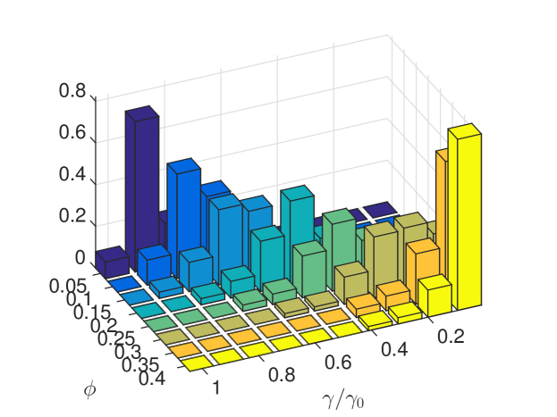
Figure 3.1: Histogram counts of $\gamma/\gamma_{0}$ for different fractions of occupied volume $\phi$ based on $100$ different crowder distributions in 2D. The radii of the crowders and the tracer are $R/\rho=0.1$ and $r/\rho=0.1$. When $0.1<\phi<0.25$ the $\gamma$-distributions are close to normal. When $\phi>0.3$ the molecule will not reach $\partial\omega_{\ast}$ implying that $E(\mathbf{x})\rightarrow\infty$ and $\gamma/\gamma_{0}\rightarrow 0$ in (2.4) for many obstacle configurations.

The effects of a deterministic $\phi(\mathbf{x})$ variable in space are studied in [52]. Sampling a new $\gamma$ for the moving molecule after $\Delta t$ accounts in [52] for the movement of the crowder molecules during that time step. This $\gamma$ sampling corresponds to the molecules switching their internal states, and we will couple the statistics in Figure 3.1 to $\mathbf{A}$ and $\mathbf{T}$ in (2.29) in the next section.

3.2 Diffusion coefficients in internal states

A molecule in different internal states $k$ in Section 2.2 has different diffusion coefficients $\gamma_{k}$ and switches its state according to $\kappa_{0}\mathbf{A}$. We sample these $\gamma_{k}$ from the stationary distributions in Section 3.1 for a given $\phi$ and the frequency of the state $k$ being $f_{k}$.

Let $\tau$ be the overall time scale for the speed of switching of the internal states and let $\kappa_{0}=1/\tau$. A large $\tau$ with $\kappa_{0}\ll\gamma_{0}$ implies that the time scale of switching the internal states is slower than the scale of diffusion. A physical interpretation is that the crowding obstacles move slowly and the tracer hence diffuses with the same $\gamma_{k}$ for a long time. If instead $\tau$ is small, then the motion of the obstacles is fast compared to the tracer molecules.

The quotient between the diffusion coefficient with crowding $\gamma_{k}$ in internal state $k$ obtained by coarse-graining and the coefficient $\gamma_{0}$ in free space is denoted by $\theta_{k}=\gamma_{k}/\gamma_{0}\in[0,1]$. The diffusion in the $k$th internal state in (2.25), (2.26), and (2.27) is

$$\gamma_{k}=\gamma_{0}\theta_{k}=\gamma_{0}T_{kk}.$$ (3.1)

Hence, $T_{kk}=\theta_{k}$. Let the ordering of the internal states be such that $\gamma_{k}<\gamma_{k+1}$.

The stationary distribution in the internal states is $\mu_{k}/T_{kk}=\mu_{k}/\theta_{k},\;k=1,\ldots,K,$ in (2.14) and (2.23). We now set this stationary distribution proportional to the frequency $f_{k}$ of the state $k$ computed by the homogenization in Section 3.1

$$\frac{\mu_{k}}{\theta_{k}}\propto f_{k},$$

and after normalizing with $\sum_{j=1}^{K}\mu_{j}=1$ we obtain

$$\mu_{k}=\frac{f_{k}\theta_{k}}{\sum_{j=1}^{K}f_{j}\theta_{j}}.$$ (3.2)

The transfer matrix in (2.12) and (2.23) is defined by

$$A_{ij}=\mu_{i}\theta_{j},\;i\neq j,\quad A_{ii}=(\mu_{i}-1)\theta_{i},$$ (3.3)

as in [45]. The stationary probability $p_{k}=p(\gamma_{k}|\phi)$ to be in internal state $k$ is proportional to $f_{k}$ and $\mu_{k}/\theta_{k}$. With a scaling such that $\sum_{j=1}^{K}p_{j}=1$, we have

$$p_{k}=\frac{f_{k}}{\sum_{j=1}^{K}f_{j}}=\frac{\mu_{k}/\theta_{k}}{\sum_{j=1}^{K}\mu_{j}/\theta_{j}}.$$ (3.4)

Using (3.1) and (3.4) the expected diffusion rate for a molecule in the stationary state is

$$\bar{\gamma}=\sum_{j=1}^{K}\gamma_{j}p_{j}=\gamma_{0}\frac{\sum_{j=1}^{K}f_{j}\theta_{j}}{\sum_{j=1}^{K}f_{j}}\leq\gamma_{0},$$ (3.5)

and the variance scaled by the square of the mean is

$$\frac{{\rm Var}[\gamma]}{\bar{\gamma}^{2}}=\bar{\gamma}^{-2}\sum_{j=1}^{K}(\gamma_{j}-\bar{\gamma})^{2}p_{j}=\sum_{j=1}^{K}\frac{\mu_{j}}{\theta_{j}}\sum_{j=1}^{K}\mu_{j}\theta_{j}-1.$$ (3.6)

The mean diffusion coefficient $\bar{\gamma}$ in (3.5) is reduced compared to diffusion in free space $\gamma_{0}$ if at least one $\theta_{k}<1$. Both $\mathbf{A}$ in (3.3) and $\bar{\gamma}$ in (3.5) are determined uniquely by $\gamma_{k}$ and the corresponding $f_{k}$.

The statistics in Figure 3.1 can be used to introduce more internal states to represent also different crowding densities $\phi_{j}$. Both $\gamma_{i}$ and $\phi_{j}$ are then sampled from the joint distribution by changing the internal states.

The frequencies $f_{k}$ for $\phi=0.2$ and $\gamma_{k}/\gamma_{0}$ determine $\theta_{k}$, $p_{k}$, and $\mu_{k}$ in ten bins in an example in Figure 3.2 using the statistics in Figure 3.1. Since $\mu_{k}$ is proportional to $f_{k}$ in (3.2), $\mu_{k}$ has the same support and is similar to $p_{k}$ in the bins. With this $\mathbf{p}$, the distribution of $\gamma$ is well approximated by a normal distribution $\mathcal{N}(\bar{\gamma},{\rm Var}[\gamma])$ with the mean and variance in (3.5) and (3.6).

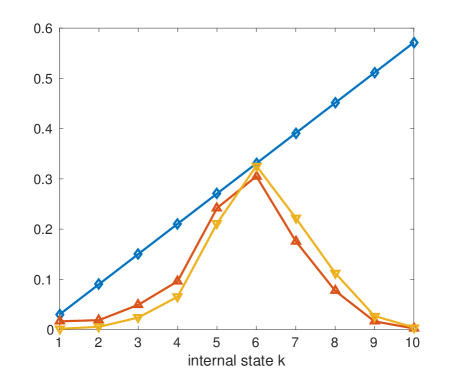
Figure 3.2: The computed $\theta_{k}\propto\gamma_{k}$ ($\diamond$, blue), $p_{k}$ ($\triangle$, red), and $\mu_{k}$ ($\nabla$, orange) for $k=1,\ldots,10,$ at $\phi=0.2$ in 2D.

4 Analytical distributions

Consider an open chemical system with the monomolecular reactions degradation, conversion, and production from a source and include diffusion between voxels $i$ and $j$ and a switch of internal states between $k$ and $l$. Then the transformations of the species are

$$A_{ik}\mathop{\rightleftharpoons}A_{jk},\;A_{ik}\mathop{\rightleftharpoons}A_{il},\;A_{ik}\longrightarrow B_{ik},\;A_{ik}\longrightarrow\emptyset,\;\emptyset\longrightarrow A_{ik}.$$ (4.1)

In order from left to right the reactions in (4.1) are: change of voxel by diffusion, change of internal state in a voxel, conversion from $A$ to $B$ in the same voxel and internal state, degradation of $A$, and production of $A$. When the reaction propensities are independent of or linear in the copy numbers, the expression for the probability distribution of molecules solving the reaction-diffusion master equation is known explicitly at the stochastic, mesoscopic level of modeling, see [51, 53]. The analytical solutions of the PDFs of the chemical networks in (4.1) are in this section used to derive the macroscopic diffusion coefficient in (2.36) and the statistical properties of the random molecular numbers of the species in the steady state.

A random vector $\mathbf{Y}$ with entries $Y_{ik\ell}$ is the state vector for the copy number of species $\ell$ in internal state $k$ in voxel $i$. The mean value of $\mathbf{Y}$ is denoted by $\bar{\mathbf{y}}$ in Section 2.2.2. We determine the probability distribution of $\mathbf{Y}$ analytically for the transformations in (4.1).

If the chemical system has the monomolecular reactions conversion and degradation as in (4.1) except for the production of $A$, then the system is closed and $\mathbf{f}$ in (2.40) in voxel $i$ in internal state $k$ is

$$\mathbf{f}(\bar{\mathbf{y}}_{ik})=\mathbf{R}\bar{\mathbf{y}}_{ik},$$ (4.2)

where $\mathbf{R}$ is constant and $\mathbf{R}\in\mathbb{R}^{L\times L}$. For such an $\mathbf{f}$ we have the stationary solution $\bar{\mathbf{y}}_{ik\infty}$ satisfying

$$\mathbf{R}\bar{\mathbf{y}}_{ik\infty}=\mathbf{0}.$$ (4.3)

Initially, there are $N$ molecules in the system. If $\emptyset$ is regarded as a special species, then the number of molecules $N$ is constant. No molecules are created and no molecules disappear. If there is degradation, the system may end up with all molecules in $\emptyset$.

The PDF of the multinomial distribution $\mathcal{M}(N,\mathbf{p})$ for $\mathbf{y}$ with $M=JKL$ states is

$$p_{\mathcal{M}}(\mathbf{y},\mathbf{p})=\frac{N!}{y_{1}!\cdot y_{2}!\cdots y_{M}!}p_{1}^{y_{1}}p_{2}^{y_{2}}\cdots p_{M}^{y_{M}},\;\sum_{m=1}^{M}y_{m}=N.$$ (4.4)

Here $m$ is the global index $m=1+(j-1)+(k-1)J+(l-1)JK$ for the state $jkl$ to simplify the notation. The probability for a molecule to be in state $m$ at $t$ is $p_{m}(t)$ and hence $\sum_{m=1}^{M}p_{m}=1,\;p_{m}\geq 0.$ Assume that the initial distribution of $\mathbf{Y}$ at $t=0$ in the chemical system is $\mathcal{M}(N,\mathbf{p}_{0})$. Then it is proved in [53] that the joint distribution of $\mathbf{Y}$ for all molecules for $t>0$ is multinomial ${\mathcal{M}}(N,\mathbf{p}(t))$ where $\mathbf{p}(t)$ solves

$$\frac{d\mathbf{p}}{dt}=\mathbf{B}\mathbf{p},\quad\mathbf{B}=\gamma_{0}\boldsymbol{\Lambda}\otimes\mathbf{T}\otimes\mathbf{I}_{L}+\kappa_{0}\mathbf{I}_{J}\otimes\mathbf{A}\otimes\mathbf{I}_{L}+\mathbf{I}_{J}\otimes\mathbf{G}\otimes\mathbf{R},$$ (4.5)

with initial data $\mathbf{p}(0)=\mathbf{p}_{0}$. The system matrix $\mathbf{B}$ is identical to the one in (2.40) where

$$\mathbf{e}_{J}\otimes\mathbf{g}\otimes\mathbf{f}=\mathbf{I}_{J}\otimes\mathbf{G}\otimes\mathbf{R}\mathbf{p}$$

for our monomolecular reactions.

Let $\mathcal{W}_{w},\,w=1,\ldots,W,$ be subsets of $\mathcal{I}_{M}=\{1,2,\ldots,M\}$ such that $\bigcup_{w=1}^{W}\mathcal{W}_{w}=\mathcal{I}_{M}$ and introduce

$$Z_{w}=\sum_{m\in\mathcal{W}_{w}}Y_{m},\quad q_{w}=\sum_{m\in\mathcal{W}_{w}}p_{m},\quad\mathbf{z}\in\mathbb{R}^{W}.$$ (4.6)

Then by the properties of the multinomial distribution, the PDF of $\mathbf{Z}$ is

$$P(t,\mathbf{z})=p_{\mathcal{M}}(\mathbf{z},\mathbf{q}(t)).$$ (4.7)

In particular, if $\mathbf{z}\in\mathbb{N}^{2}$, i.e. $W=2$ and $z_{w}$ is integer and non-negative, then the distribution is binomial.

The stationary distribution when $t\rightarrow\infty$ is

$$\lim_{t\rightarrow\infty}P(t,\mathbf{y})=p_{\mathcal{M}}(\mathbf{y},\mathbf{p}_{\infty}),$$ (4.8)

where $\mathbf{p}_{\infty}$ is the solution of

$$\mathbf{B}\mathbf{p}_{\infty}=0.$$ (4.9)

The vectors $\mathbf{v}$ and $\mathbf{T}^{-1}\boldsymbol{\mu}$ satisfy $\boldsymbol{\Lambda}\mathbf{v}=\mathbf{0}$ and $\mathbf{A}\mathbf{T}^{-1}\boldsymbol{\mu}=\mathbf{0}$ as in (2.34). Let $\mathbf{p}_{\Lambda\infty},\mathbf{p}_{A\infty},$ and $\mathbf{p}_{R\infty}$ satisfy

$$\mathbf{p}_{\Lambda\infty}=\eta_{\Lambda}\mathbf{v},\;\mathbf{p}_{A\infty}=\eta_{A}\mathbf{T}^{-1}\boldsymbol{\mu},\;\mathbf{R}\mathbf{p}_{R\infty}=\mathbf{0},$$ (4.10)

with $\mathbf{p}_{R\infty}$ and scalings $\eta_{\Lambda}$ and $\eta_{R}$ chosen to fulfill $\|\mathbf{p}_{\Lambda\infty}\|_{1}=\|\mathbf{p}_{A\infty}\|_{1}=\|\mathbf{p}_{R\infty}\|_{1}=1$. The stationary distributions $\mathbf{p}_{\Lambda\infty},\mathbf{p}_{A\infty},$ and $\mathbf{p}_{R\infty}$ are all independent of $\gamma_{0}$ and $\kappa_{0}$. If the reaction matrix $\mathbf{R}$ is irreducible such that the chemical network cannot be decomposed into two or more independent networks, then there is a $\mathbf{p}_{R\infty}$ with non-negative components $p_{R\infty,i}$ in (4.10) [51, 53]. It follows from (4.9), (4.5), and (4.10) that

$$\mathbf{p}_{\infty}=\mathbf{p}_{\Lambda\infty}\otimes\mathbf{p}_{A\infty}\otimes\mathbf{p}_{R\infty},\;\|\mathbf{p}_{\infty}\|_{1}=1.$$ (4.11)

With the conversion reaction in (4.1), $\mathbf{R}$ is such that $\mathbf{e}_{L}^{T}\mathbf{R}=\mathbf{0}$. It follows from (2.31) and (4.5) that

$$(\mathbf{e}_{J}\otimes\mathbf{e}_{K}\otimes\mathbf{e}_{L})^{T}\mathbf{B}=\mathbf{0}.$$ (4.12)

Using (4.5), we find that

$$(\mathbf{e}_{J}\otimes\mathbf{e}_{K}\otimes\mathbf{e}_{L}^{T}\mathbf{p})_{t}=(\mathbf{e}_{J}\otimes\mathbf{e}_{K}\otimes\mathbf{e}_{L})^{T}\mathbf{p}_{t}=\mathbf{0},$$ (4.13)

and the probability is preserved

$$\|\mathbf{p}(t)\|_{1}=\|\mathbf{p}(0)\|_{1}=\|\mathbf{p}_{\infty}\|_{1}=1,$$ (4.14)

with a properly chosen initial solution $\mathbf{p}_{0}=\mathbf{p}(0)$.

When the time scale of the diffusion is fast with a large $\tau=\kappa_{0}^{-1}\gg\gamma_{0}^{-1}$, then by (3.3) $\kappa_{0}\mathbf{A}$ is negligible in (4.5) since $\mathbf{A}$ is of $\mathcal{O}(1)$. Spatial gradients disappear rapidly and the system is well-stirred. On the contrary, if $\tau$ is small then $\kappa_{0}\mathbf{A}$ dominates and there is a fast equilibration in the internal states such that the solution is (after reordering the unknowns $p_{ik\ell}$) $\mathbf{p}(t)\approx\mathbf{p}^{\prime}(t)\otimes\mathbf{p}_{A\infty}$ and $\mathbf{I}_{J}\otimes\mathbf{I}_{L}\otimes\mathbf{A}\mathbf{p}\approx(\mathbf{I}_{J}\otimes\mathbf{I}_{L})\mathbf{p}^{\prime}\otimes\mathbf{A}\mathbf{p}_{A\infty}=\mathbf{0}$ in the second term in $\mathbf{B}$ in (4.5).

The expected value $u_{ik\ell}$ of the concentration of species $\ell$ in voxel $i$ and internal state $k$ is given by

$$u_{ik\ell}(t)=E\left[\frac{Y_{ik\ell}}{|\mathcal{V}_{i}|}\right]=\frac{N}{|\mathcal{V}_{i}|}p_{ik\ell}(t)=\frac{\bar{y}_{ikl}}{|\mathcal{V}_{i}|}.$$ (4.15)

Since the mean values of the copy numbers $\overline{\mathbf{y}}(t)$ satisfy (4.5), $\mathbf{u}$ in (4.15) satisfies an equation like (2.25) with an additional reaction term.

The diffusion coefficient in the equation for the observable $U_{i\ell}$ in (2.37) in voxel $i$ and species $\ell$ with $\mathbf{e}^{T}_{K}\mathbf{p}_{i\ell}(t)>0$ is by (2.36), (4.15), and (3.1)

$$\hat{\gamma}_{i\ell}(t)=\gamma_{0}\frac{\mathbf{e}^{T}_{K}\mathbf{T}\mathbf{p}_{i\ell}(t)}{\mathbf{e}^{T}_{K}\mathbf{p}_{i\ell}(t)}=\gamma_{0}\frac{\sum_{k=1}^{K}\theta_{k}p_{ik\ell}(t)}{\sum_{k=1}^{K}p_{ik\ell}(t)}\leq\gamma_{0},$$ (4.16)

since $0\leq\theta_{j}\leq 1$, cf. (3.5) for the stationary case. The time dependent diffusion coefficient $\hat{\gamma}_{i\ell}(t)$ is bounded from above by the nominal coefficient $\gamma_{0}$ and as $t\rightarrow\infty$, $\hat{\gamma}_{i\ell}(t)$ approaches $\bar{\gamma}$ in (3.5).

A simpler alternative to $\hat{\gamma}$ in (4.16) is to derive the random diffusion field in (2.37) as follows. First, discretize the time derivative in (2.37) at $t^{n},\,n=0,1,\ldots$, and sample $\hat{\gamma}_{j}^{n}$ with the stationary distribution in (3.4). Then we have a numerical approximation of the parabolic PDE (2.11) discretized by finite elements in (2.37) with a random, space and time dependent diffusion coefficient field $\tilde{\gamma}$ with mean and variance (3.5) and (3.6).

The sum of the molecules over the internal states in each voxel and for each species is denoted by

$$Z_{i\ell}=\sum_{k=1}^{K}Y_{ik\ell}.$$ (4.17)

Since $\mathbf{Y}$ is multinomially distributed with parameters $\mathbf{p}$, $\mathbf{Z}$ is also multinomially distributed $\mathcal{M}(N,\mathbf{q})$ according to (4.6) and (4.7) where $\mathbf{q}$ has the components

$$q_{i\ell}(t)=\sum_{k=1}^{K}p_{ik\ell}(t).$$ (4.18)

At the stationary distribution, $\mathbf{q}$ is

$$q_{i\ell\infty}=\sum_{k=1}^{K}p_{\Lambda\infty,i}p_{A\infty,k}p_{R\infty,\ell}=p_{\Lambda\infty,i}p_{R\infty,\ell}.$$ (4.19)

The observable $U_{i\ell}$ is the expected value of the concentration of species $\ell$ in $\mathcal{V}_{i}$

$$U_{i\ell}(t)={\rm E}\left[\frac{Z_{i\ell}}{|\mathcal{V}_{i}|}\right]=\frac{N}{|\mathcal{V}_{i}|}q_{i\ell}(t).$$ (4.20)

Using (4.19), we find that the steady state solution $U_{\infty,i\ell}$ is independent of $i$ and thus constant in space. The variance of the concentration is

$${\rm Var}\left[\frac{Z_{i\ell}}{|\mathcal{V}_{i}|}\right]=\frac{N}{|\mathcal{V}_{i}|^{2}}q_{i\ell}(t)(1-q_{i\ell}(t)).$$ (4.21)

The number of voxels $J$ is often large making $q_{i\ell}(t)\propto 1/JL$ and small and the variance is approximately $Nq_{i\ell}(t)/|\mathcal{V}_{i}|^{2}=U_{i\ell}/|\mathcal{V}_{i}|$. The covariance between species $\ell$ in voxel $i$ and species $m$ in voxel $j$ is

$${\rm Cov}\left[\frac{Z_{i\ell}}{|\mathcal{V}_{i}|},\frac{Z_{jm}}{|\mathcal{V}_{j}|}\right]=-\frac{N}{|\mathcal{V}_{i}||\mathcal{V}_{j}|}q_{i\ell}(t)q_{jm}(t).$$ (4.22)

The co-variation between the voxels is negative and since $q_{i\ell}$ is usually small, it is very small. The mean and the variance of the copy numbers $Z_{i\ell}$ are

$$E[Z_{i\ell}]=Nq_{i\ell}(t),\quad{\rm Var}[Z_{i\ell}]=Nq_{i\ell}(t)(1-q_{i\ell}(t)).$$ (4.23)

The Fano factor ${\rm Var}[Z_{i\ell}]/E[Z_{i\ell}]$ is $1-q_{i\ell}(t)$ and close to 1, which is the factor of a Poisson process.

A similar analysis is possible for a chemical system when all monomolecular reactions in (4.1) are included. If the copy numbers $\mathbf{Y}$ in the states of the system are Poisson distributed initially then they will remain Poisson distributed with rate parameters satisfying an equation like (4.5) and (2.40), see [53].

5 Numerical examples

We now proceed to illustrate the behavior of the suggested coarse-grained model of subdiffusion in stochastic simulation of trajectories of the chemical network. After first briefly summarizing the simulation algorithm in Section 5.1, we look at the mean-square displacement of subdiffusing molecules on a circle in Section 5.2 using a finite element discretization over a triangular mesh to discretize the required diffusion operator as in Section 2.2.2. In Section 5.3, we investigate the available range of dynamics when bimolecular reactions are included. Finally, in Section 5.4 we look at potential subdiffusive effects when simulating a realistic three-dimensional model of a subsystem of an E. coli model. In all examples, the mesoscopic internal states model with variable diffusion coefficients is determined as in Section 3. With repeatability and reproducibility in mind, the models tested here will be released in the coming version 1.4 of our freely available software URDME [27, 54].

5.1 Stochastic Simulation Algorithm

The direct simulation method [23] by Gillespie determines the time for the next reaction event and which event that will take place. For spatial problems the state of the chemical system is a random variable $\mathbf{Y}\in\mathbb{N}^{JKL}$ and is defined by the number of molecules of each species in the internal states in each voxel. The simulation method of choice is then the next subvolume method (NSM) [24]. The probabilities for the events are given by the coefficients in $\boldsymbol{\Lambda}\otimes\mathbf{T}$ (diffusion), $\mathbf{A}$ (change of internal state), and the reaction propensities in $\mathbf{f}$. The change of internal state in a voxel has the form of a monomolecular reaction.

The NSM algorithm becomes time-consuming with multiple internal states since many events simply change the internal states without advancing the observable dynamics. A parallel version suitable for modern multicore computers was developed in [55] which is effective in dealing with events taking place within spatial subdomains rather than between them. We remark that introducing the internal states is a way of simulating a system with a random, predetermined diffusion coefficient $\gamma(\mathbf{x},t)$. Simulation of such a system without internal states requires a special, more complicated version of Gillespie’s algorithm to handle time dependent coefficients [56].

5.2 Pure subdiffusion

There is experimental evidence that the diffusive transport of molecules in cells is sometimes anomalous [10, 6, 43]. Let $\langle\cdot\rangle$ denote the average over the trajectories of the molecules. The mean square displacement (MSD) of a molecule at $\mathbf{x}(t)$ at time $t$ released at $\mathbf{x}(0)=0$ at $t=0$ behaves as

$$\langle\|\mathbf{x}(t)\|^{2}_{2}\rangle\propto t^{\alpha},$$ (5.1)

where $\alpha=1$ for ordinary diffusion and $\alpha\in(0,1)$ in subdiffusion where, at least in a time interval shortly after $t=0$, the molecules diffuse anomalously, see [10]. The reason for the subdiffusion may be crowding effects by other molecules and the process is then non-ergodic with a memory, see e.g. [57, 40].

The macroscopic observable $\mathbf{U}(\mathbf{x},t)\in\mathbb{R}^{L}$, e.g., the concentrations of the chemical species, satisfies a diffusion equation with a fractional time derivative [43]

$${\frac{\partial\mathbf{U}}{\partial t}=\frac{\partial^{1-\alpha}}{\partial t^{1-\alpha}}(\gamma\Delta\mathbf{U}),}$$ (5.2)

at least in a time interval, $t\in[t_{0},t_{1}]$. The fractional derivative is defined according to Riemann-Liouville. The internal state parameters $\boldsymbol{\mu}$ and $\boldsymbol{\theta}$ in (3.3) are determined by $\alpha$ in the FPDE in [45, 44]. Here they are given by statistics obtained with the microscopic model in [36].

We compute the MSD (5.1) of the internal states model by coarse-graining into ten states as in Figure 3.2 following the procedure described in Section 3.2 using $\phi=0.2$ and $\gamma_{0}=0.01$. The geometry is the unit circle and the molecules are released at time $t=0$ in the center and in the fastest diffusing internal state with $\gamma_{10}=\gamma_{0}\theta_{10}$. Since there are no reactions, all transition rates act linearly and the moment equations are closed such that the mean square displacement can be accurately determined by solving (4.5) numerically for $\mathbf{p}$ with $L=1$ and $\mathbf{R}=1$ for the probability to be in voxel $i$. Then the MSD in (5.1) is $\langle\|\mathbf{x}(t)\|^{2}_{2}\rangle=\sum_{i}p_{i}(t)\|\mathbf{x}_{i}\|^{2}_{2}$ where $\mathbf{x}_{i}$ is the center of voxel $i$.

The initial diffusion rate is $\gamma_{0}\theta_{10}$ and, as $t\to\infty$, $\gamma$ converges to $\bar{\gamma}$. The region in between these two limits is where the subdiffusive behavior is observed, and where $\alpha<1$ in (5.1) and (5.2). Initially and for large $t$, $\alpha=1$ and we have ordinary diffusion. By scaling the internal transfer matrix $\mathbf{A}$ with a different $\kappa_{0}$ in (2.22), this region (indicated by the comparision slope) can be varied accordingly, see Figure 5.1, where the same $\alpha$ is obtained with two different values of $\kappa_{0}$. Recall that $\kappa_{0}$ models the speed of diffusion of the obstacles and for an accurate description their average diffusion speed should be known.

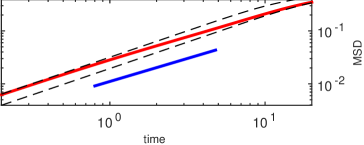
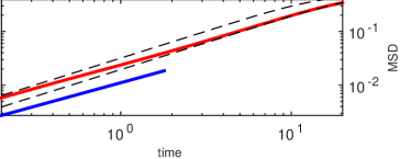
Figure 5.1: Simulation of coarse-grained subdiffusion in 2D. Top: The mean square displacement as a function of time (red). The dashed curves are obtained with the initial and the steady state diffusion, $\gamma_{0}$ and $\bar{\gamma}$, and the slope of the comparison curve $t^{\alpha}$ is $\alpha=0.87$ (blue). Bottom: As above, but with a four times faster diffusion of obstacles and hence faster scaling of time for the switching between internal states, $\kappa_{0}\rightarrow 4\kappa_{0}$, resulting in a faster approach to the steady state diffusion (but still such that $\alpha=0.87$ for the comparison slope).

5.3 Bimolecular annihilation

Consider two species $A$ and $B$ undergoing the single transition

$$A_{i}+B_{j}\to C,$$ (5.3)

with $A$ in the internal state $i$ and $B$ in $j$ and with an arbitrary internal state for $C$. Let the rate for this transition be $H_{ij},\;i,j=1,\ldots,K$. Then the reaction propensity is $H_{ij}a_{i}b_{j}$ where $a_{i}$ and $b_{j}$ are the copy numbers of $A_{i}$ and $B_{j}$. Given an arbitrary non-negative rate matrix $\mathbf{H}$, a steady state probability distribution $\mathbf{p}_{A\infty}$ of the internal states for both $A$ and $B$, and a target rate constant $k_{0}$, we can always scale $\mathbf{H}$ such that the mean rate agrees with the target at the steady state

$$k_{0}=\mathbf{p}_{A\infty}^{T}\mathbf{H}\mathbf{p}_{A\infty}.$$ (5.4)

There is potentially great freedom in selecting the rate parameters subject to a scaling. Note that when $H_{ij}$ is independent of $i$ and $j$ and $\mathbf{H}=k_{0}\mathbf{e}_{L}\mathbf{e}_{L}^{T}$, the internal states model agrees with the standard model using a single target rate $k_{0}$. The diffusion in the internal states is as in the previous example.

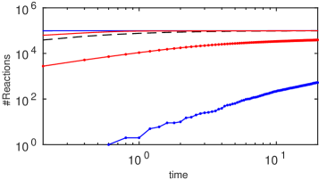
Figure 5.2: Results of the bimolecular reaction in (5.3) presented as the time history of the number of resulting molecules $C$. The colored lines represent simulations with $H_{ij}$ in the different cases 1 (blue with dots), 2 (red with dots), 3 (smooth red), and 4 (smooth blue), respectively. The dashed line is the pure diffusion case with $k_{0}$ as the single rate.

We release $A$ and $B$ molecules at time $t=0$, $10^{5}$ of each species, in ten internal states uniformly in space in the unit disc with all in the fastest (the tenth) diffusing state. Four different cases of rate parameters are defined as follows:

1. $H_{1,1}=1$ and 0 otherwise,

2. $H_{ij}=(11-i)(11-j)$,

3. $H_{ij}=ij$,

4. $H_{10,10}=1$ and 0 otherwise.

Then the parameters are rescaled such that $\mathbf{H}$ satisfies (5.4) with $k_{0}=10^{-4}$. In cases 1 and 4, two molecules $A$ and $B$ react only when they both are in the same voxel and in the same internal state. The reaction rate decreases or increases with the diffusion in cases 2 and 3. The combined effect of internal states and reactions is modeled by $\mathbf{H}$ corresponding to $\mathbf{g}\otimes\mathbf{f}$ in (2.40).

The result obtained from a single realization of the system with URDME, visualized as the number of resulting $C$ molecules, is displayed in Figure 5.2. The extreme cases 1 and 4 where a single rate in $\mathbf{H}$ is non-zero are clearly identifiable, as are the two intermediate cases 2 and 3. The single state model is found in the middle of all of these cases. Different choices of reaction rates yield a range of behavior. The idea that there is a freedom in selecting the rate parameters opens up for advanced coarse-graining methods based on, e.g., analytic and simulation results in the diffusion-limited regime [58, 59, 2], or computational methods based on data from Brownian dynamics [37, 38] or molecular dynamics [60] simulations.

5.4 Min oscillations in E. coli

As a more involved example in three space dimensions, we take the model from [61] of the Min-system in the E. coli bacterium. The geometry is rod-shaped with length $3.5\mu m$, diameter $1\mu m$, and discretized using 9761 tetrahedra, see Figure 5.3. MinD proteins oscillate from pole to pole in the cell with a low concentration in the middle. These oscillations help the cell locate its middle before cell division [62]. The five reactions, five species, and reaction parameters from [61] are found in Table 5.1. Two of the species, MinDmem and MinDE, are attached to the membrane and only diffuse there. The other three species diffuse freely in the cytosol, where the effective diffusion constant is $\gamma_{0}=2.5\mu m^{2}/s$ in [61]. Since the inside of an E. coli is a highly crowded environment (cf. Figure 1.1), it is of interest to investigate the incorporation of subdiffusion due to crowding and reaction rates depending on the internal state in the mesoscopic model.

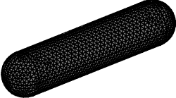
Figure 5.3: A discretized model of an E. coli bacterium.

$\mbox{MinDcytATP}\xrightarrow{k_{d}}\mbox{MinDmem}$	$\mbox{MinDcytATP}+\mbox{MinDmem}\xrightarrow{k_{dD}}\mbox{2MinDmem}$
$\mbox{MinE+MinDmem}\xrightarrow{k_{de}}\mbox{MinDE}$	$\mbox{MinDE}\xrightarrow{k_{e}}\mbox{MinDcytADP}+\mbox{MinE}$
$\mbox{MinDcytADP}\xrightarrow{k_{p}}\mbox{MinDcytATP}$

Table 5.1: The chemical reactions of the Min-system. The constants take the values $k_{d}=0.0125\mu m^{-1}s^{-1}$, $k_{dD}=9\times 10^{6}M^{-1}s^{-1}$ (here scaled by an additional factor of 1.65 in the numerical experiments), $k_{de}=5.56\times 10^{7}M^{-1}s^{-1}$, $k_{e}=0.7s^{-1}$, and $k_{p}=0.5s^{-1}$.

As a proof-of-concept and in order to demonstrate the possibilities here, we scaled the critical binding reaction rate $k_{dD}$ by a factor 1.65, thus bringing the kinetics into a more sensitive regime compared to the original rate. The normally diffusing model then displays stable oscillations of the $Min$-protein in the membrane (see upper left panel in Figure 5.4).

As in the previous experiments we employ ten internal states obtained from coarse-graining at $\phi=0.2$. For the binding reaction of state $i$, we multiply $k_{dD}$ by a factor $1+0.03i$ meaning that the reactivity increases with faster diffusion. We then rescale the resulting rate as in (5.4) such that the steady state mean rate agrees with the single state model. To bring in a bias we arbitrarily let all reactions produce products in the fastest diffusing state with $i=10$ ($A_{i}+B_{j}\to C_{10},\,\forall i,j$ where $1\leq i,j\leq 10$), thus skewing the distribution over the internal states towards faster diffusion and also faster binding rate. The presence of subdiffusion and variable reaction rates in this model has a striking effect on the oscillatory behavior. The oscillations are damped considerably, see the lower left panel in Figure 5.4. The peak in the power spectrum at about $0.03Hz$ in the right panel of Figure 5.4 is reduced by more than a factor 6 in the internal state model. With our computational framework, an investigation of the dynamics due to crowding and variable reaction rates is computationally feasible even in non-trivial and quite large examples.

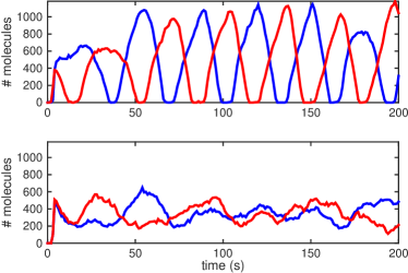
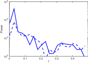
Figure 5.4: Two realizations of MinD-oscillations in the membrane of an E. coli bacterium. Left: The number of MinD molecules in the leftmost (red) and rightmost (blue) quarters of the bacterium, respectively. Top: Ordinary diffusion without internal states. Bottom: Our coarse-grained subdiffusion model. Right: The Fourier power spectrum of the pole oscillations of the two models : ordinary diffusion (solid) and coarse-grained subdiffusion (dashed).

6 Conclusions

We have developed a computationally efficient approach to simulate diffusive and subdiffusive transport processes on the mesoscopic level taking the explicit description of obstacle sizes and densities into account. We therefore couple two existing methods: the internal states model and the coarse-graining of a microscopic crowded geometry to the mesoscopic level, see the summary in Figure 6.1. Our novel method is faster than directly simulating microscopic Brownian dynamics and permits more detailed modeling than a standard mesoscopic model with fixed diffusion and reaction coefficients. In other lattice methods for simulation of crowding, only a limited number of molecules can occupy the same voxel in the lattice. Compared to those methods, our method is less heuristic and models the effect of crowding by deriving a distribution of diffusion coefficients from a fine-grain geometry with obstacles of different shape and size.

An observable is the sum of the copy numbers in all internal states. The mean values of the copy numbers of the observables satisfy macroscopic PDEs discretized by a finite element method. The diffusion in the PDE for the observables is not explicitly known unless the mean values of the full mesoscopic system are known.

The crowding model has been implemented in URDME [27, 54] and examples in 2D and 3D show the effects of crowding and the modeling of the reactions. The mean square displacement of a diffusing molecule is computed and the $\alpha$ parameter measuring the deviation from Brownian motion is recorded. Subdiffusive behavior is observed in a time interval after release of the molecule. The reaction propensities vary with the internal state in two examples. The scaling of the reaction coefficients is such that the same steady state is reached but the transient phase differs in the simulations depending on the particular choice of internal representation. This is illustrated in one example. In the other example, a realization of the MinD system without internal states is oscillatory but is irregular with an internal structure in the voxels.

The data for calibration of the internal states are here taken from homogenization of a detailed microscopic model of crowding but other sources are also possible. One alternative would be to infer the diffusion and reaction rates from the posterior distribution of a Bayesian approach to analysis of experimental data. Another possibility would be to obtain the rates from coarse-graining data from Brownian dynamics or molecular dynamics realizations of diffusion and reactions.

Microscopic and detailed computational methods are very expensive for simulation of biochemical networks and are restricted to smaller subsystems and for short time. Our mesoscopic method including microscopic data offers a fast and accurate approach for larger systems and longer time intervals at a much reduced computational cost.

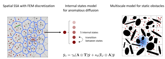
Figure 6.1: Summary of the method. Left: A triangulation (grey edges) between the nodes $\mathbf{x}_{j}$ defines the primal mesh and the dual mesh (blue boundaries) which forms the voxels $\mathcal{V}_{j}$. Red and black tracer molecules diffuse (red arrows) between voxels. They react with each other (green arrow) when they are located in the same voxel. Middle: The molecules in a voxel are in $K$ internal states ($K=5$ here). In the equation for the mean values $\bar{\mathbf{y}}$ of the number of molecules in each state in every voxel, $\gamma_{0}$ is the free diffusion coefficient, $\boldsymbol{\Lambda}$ is the matrix of jump coefficients between the voxels given by a finite element discretization, $\mathbf{T}$ scales the hindered diffusion due to crowding in the $K$ internal states, $1/\kappa_{0}$ determines the time scale of the internal jumps, and $\mathbf{A}$ is the matrix of jump coefficients between the internal states in a voxel. Right: The jump rates between the internal states in $\mathbf{A}$ are determined by computing the mean first exit time from the blue circle for a red tracer molecule with black obstacle molecules. Statistics is collected for many different obstacle configurations. Sampling from this distribution means that the tracer molecule is experiencing different crowder densities and consequently changes its internal state. Summary: The novelty of our approach lies in coupling the internal states model (middle) which has previously been used to simulate anomalous diffusion to the explicit description of crowder molecules by coarse-graining the microscopic information to the mesoscopic level (right).

References

- [1] K. Luby-Phelps. Cytoarchitecture and physical properties of cytoplasm: volume, viscosity, diffusion, intracellular surface area. Int. Rev. Cytology, 192:189–221, 1999.
- [2] S. Schnell and T. E. Turner. Reaction kinetics in intracellular environments with macromolecular crowding: Simulations and rate laws. Prog. Biophys. Mol. Biol., 85(2-3):235–260, 2004.
- [3] P. R. ten Wolde and A. Mugler. Importance of crowding in signaling, genetic, and metabolic networks. Int. Rev. Cell Mol. Bio., 307:419–442, 2014.
- [4] B. Grasberger, A. P. Minton, C. DeLisi, and H. Metzger. Interaction between proteins localized in membranes. Proc. Natl. Acad. Sci. USA, 83(17):6258–6262, 1986.
- [5] S. Jin and A. S. Verkman. Single particle tracking of complex diffusion in membranes: Simulation and detection of barrier, raft, and interaction phenomena. J. Phys. Chem. B, 111(14):3625–3632, 2007.
- [6] D. Krapf. Mechanisms underlying anomalous diffusion in the membrane. Curr. Topics Membr., 75:167–207, 2015.
- [7] O. Medalia, I. Weber, A. S. Frangakis, D. Nicastro, G. Gerisch, and W. Baumeister. Macromolecular architecture in eukaryotic cells visualized by cryoelectron tomography. Science, 298(5596):1209–1213, 2002.
- [8] C. Di Rienzo, V. Piazza, E. Gratton, F. Beltram, and F. Cardarelli. Probing short-range protein Brownian motion in the cytoplasm of living cells. Nat. Commun., 5:5891, 2014.
- [9] M. Galanti, D. Fanelli, A. Maritan, and F. Piazza. Diffusion of tagged particles in a crowded medium. Europhys. Lett., 107(2):20006, 2014.
- [10] F. Höfling and T. Franosch. Anomalous transport in the crowded world of biological cells. Rep. Progr. Phys., 76:046602, 2013.
- [11] D. V. Nicolau Jr, J. F. Hancock, and K. Burrage. Sources of anomalous diffusion on cell membranes: A Monte Carlo study. Biophys. J., 92:1975–1987, 2007.
- [12] D. Hall and A. P. Minton. Macromolecular crowding: Qualitative and semiquantitative successes, quantitative challenges. Biochim. Biophys. Acta - Proteins Proteomics, 1649(2):127–139, 2003.
- [13] T. Ando and J. Skolnick. Crowding and hydrodynamic interactions likely dominate in vivo macromolecular motion. Proc. Natl. Acad. Sci. USA, 107(43):18457–18462, 2010.
- [14] C. J. Penington, B. D. Hughes, and K. A. Landman. Building macroscale models from microscale probabilistic models: A general probabilistic approach for nonlinear diffusion and multispecies phenomena. Phys. Rev. E, 84(4):041120, 2011.
- [15] M. J. Saxton. A biological interpretation of transient anomalous subdiffusion. I. Qualitative model. Biophys. J., 92:1178–1191, 2007.
- [16] S. B. Yuste, L. Acedo, and K. Lindenberg. Reaction front in an reaction-subdiffusion process. Phys. Rev. E, 69:036126, 2004.
- [17] D. J. Kiviet, P. Nghe, N. Walker, S. Boulineau, V. Sunderlikova, and S. J. Tans. Stochasticity of metabolism and growth at the single-cell level. Nature, 514:376–379, 2014.
- [18] H. H. McAdams and A. Arkin. Stochastic mechanisms in gene expression. Proc. Natl. Acad. Sci. USA, 94(3):814–819, Feb. 1997.
- [19] J. M. Pedraza and A. van Oudenaarden. Noise propagation in gene networks. Science, 307(5717):1965–1969, Mar. 2005.
- [20] V. Shahrezaei and P. S. Swain. The stochastic nature of biochemical networks. Curr. Op. Biotech., 19:369–374, 2008.
- [21] P. S. Swain, M. B. Elowitz, and E. D Siggia. Intrinsic and extrinsic contributions to stochasticity in gene expression. Proc. Natl. Acad. Sci. USA, 99(20):12795–12800, Oct. 2002.
- [22] N. G. van Kampen. Stochastic Processes in Physics and Chemistry. Elsevier, Amsterdam, 2nd edition, 2004.
- [23] D. T. Gillespie. A general method for numerically simulating the stochastic time evolution of coupled chemical reactions. J. Comput. Phys., 22(4):403–434, 1976.
- [24] J. Elf and M. Ehrenberg. Spontaneous separation of bi-stable biochemical systems into spatial domains of opposite phases. Syst. Biol. IEE Proc., 1(2):230–236, 2004.
- [25] J Hattne, D Fange, and J Elf. Stochastic reaction-diffusion simulation with MesoRD. Bioinformatics, 21(12):2923–2924, 2005.
- [26] S. A. Isaacson and C. S. Peskin. Incorporating diffusion in complex geometries into stochastic chemical kinetics simulations. SIAM J. Sci. Comput., 28:47–74, 2006.
- [27] B. Drawert, S. Engblom, and A. Hellander. URDME: a modular framework for stochastic simulation of reaction-transport processes in complex geometries. BMC Syst. Biol., 6(76):1–17, 2012.
- [28] S. Engblom, L. Ferm, A. Hellander, and P. Lötstedt. Simulation of stochastic reaction-diffusion processes on unstructured meshes. SIAM J. Sci. Comput., 31:1774–1797, 2009.
- [29] K. Burrage, P. Burrage, A. Leier, and T. Marquez-Lago. A review of stochastic and delay simulation approaches in both time and space in computational cell biology. In D. Holcman, editor, Stochastic Processes, Multiscale Modeling, and Numerical Methods for Computational Cellular Biology, pages 241–261, Cham, 2017. Springer.
- [30] S. Engblom, A. Hellander, and P. Lötstedt. Multiscale simulation of stochastic reacion-diffusion networks. In D. Holcman, editor, Stochastic Processes, Multiscale Modeling, and Numerical Methods for Computational Cellular Biology, pages 55–79, Cham, 2017. Springer.
- [31] A. Mahmutovic, D. Fange, O. G. Berg, and J. Elf. Lost in presumption: stochastic reactions in spatial models. Nat. Meth., 9(12):1–4, 2012.
- [32] E. Roberts, J. E. Stone, and Z. Luthey-Schulten. Lattice microbes: High-performance stochastic simulation method for the reaction-diffusion master equation. J. Comput. Chem., 34(3):245–255, 2013.
- [33] D. Fanelli and A. J. McKane. Diffusion in a crowded environment. Phys. Rev. E, 82(2):021113, 2010.
- [34] K. A. Landman and A. E. Fernando. Myopic random walkers and exclusion processes: Single and multispecies. Phys. A, Stat. Mech. Appl., 390(21-22):3742–3753, 2011.
- [35] P. R. Taylor, C. A. Yates, M. J. Simpson, and R. E. Baker. Reconciling transport models across scales: The role of volume exclusion. Phys. Rev. E, 92(4):040701, 2015.
- [36] L. Meinecke. Multiscale modeling of diffusion in a crowded environment. Bull. Math. Biol., 79:2672–2695, 2017.
- [37] S. S. Andrews, N. J. Addy, R. Brent, and A. P. Arkin. Detailed simulations of cell biology with Smoldyn 2.1. PLoS Comput. Biol., 6(3):e1000705, 2010.
- [38] J. S. van Zon and P. R. ten Wolde. Green’s-function reaction dynamics: A particle-based approach for simulating biochemical networks in time and space. J. Chem. Phys., 123:234910, 2005.
- [39] S. Smith and R. Grima. Fast simulation of Brownian dynamics in a crowded environment. J. Chem. Phys., 146:024105, 2017.
- [40] T. T. Marquez-Lago, A. Leier, and K. Burrage. Anomalous diffusion and multifractional Brownian motion: simulating molecular crowding and physical obstacles in systems biology. IET Syst. Biol., 6(4):134–142, 2012.
- [41] L. Meinecke and M. Eriksson. Excluded volume effects in on- and off-lattice reaction-diffusion models. IET Syst. Biol., 11(2):55–64, 2017.
- [42] E. Barkai, Y. Garini, and R. Metzler. Strange kinetics of single molecules in living cells. Physics Today, 65(8):29–35, 2012.
- [43] R. Metzler and J. Klafter. The random walk’s guide to anomalous diffusion: a fractional dynamics approach. Phys. Rep., 339(1):1–77, 2000.
- [44] M. S. Mommer and D. Lebiedz. Modeling subdiffusion using reaction diffusion systems. SIAM J. Appl. Math., 70(1):112–132, 2009.
- [45] E. Blanc, S. Engblom, A. Hellander, and P. Lötstedt. Mesoscopic modeling of stochastic reaction-diffusion kinetics in the subdiffusive regime. Multiscale Model. Simul., 14:668–707, 2016.
- [46] F. Persson, M. Lindén, C. Unoson, and J. Elf. Extracting intracellular diffusive states and transition rates from single molecule tracking data. Nat. Meth., 10:265–269, 2013.
- [47] B. Øksendal. Stochastic Differential Equations. Springer, Berlin, 6th edition, 2003.
- [48] M. D. Gunzburger, C. G. Webster, and G. Zhang. Stochastic finite element methods for partial differential equations with random input data. Acta Numerica, pages 521–650, 2014.
- [49] P. Lötstedt and L. Meinecke. Simulation of stochastic diffusion via first exit times. J. Comput. Phys., 300:862–886, 2015.
- [50] L. Meinecke, S. Engblom, A. Hellander, and P. Lötstedt. Analysis and design of jump coefficients in discrete stochastic diffusion models. SIAM J. Sci. Comput., 38:A55–A83, 2016.
- [51] C. Gadgil, C. H. Lee, and H. G. Othmer. A stochastic analysis of first-order reaction networks. Bull. Math. Biol., 67:901–946, 2005.
- [52] S. Smith, C. Cianci, and R. Grima. Macromolecular crowding directs the motion of small molecules inside cells. J. R. Soc. Interface, 14:20170047, 2017.
- [53] T. Jahnke and W. Huisinga. Solving the chemical master equation for monomolecular reaction systems analytically. J. Math. Biol., 54:1–26, 2007.
- [54] S. Engblom et al. URDME: Unstructured Reaction-Diffusion Master Equation, 2008–2017. Multiple versions exist. Available at www.urdme.org.
- [55] J. Lindén, P. Bauer, S. Engblom, and B. Jonsson. Exposing inter-process information for efficient parallel discrete event simulation of spatial stochastic systems. ACM SIGSIM-PADS, Singapore, May 24–26, 2017.
- [56] M. A. Gibson and J. Bruck. Efficient exact stochastic simulation of chemical systems with many species and many channels. J. Phys. Chem., 104(9):1876–1889, 2000.
- [57] R. Hilfer and L. Anton. Fractional master equations and fractal time random walks. Phys. Rev. E, 51(2):R848–R851, 1995.
- [58] R. Grima and S. Schnell. A systematic investigation of the rate laws valid in intracellular environments. Biophys. Chem., 124:1–10, 2006.
- [59] B. J. Henry, T. A. M. Langlands, and S. L. Wearne. Anomalous diffusion with linear reaction dynamics: From continuous time random walks to fractional reaction-diffusion equations. Phys. Rev. E, 74:031116, 2006.
- [60] S. Pronk, S. Páll, R. Schulz, P. Larsson, P. Bjelkmar, R. Apostolov, M. R. Shirts, J. C. Smith, P. M. Kasson, D. van der Spoel, B. Hess, and E. Lindahl. GROMACS 4.5: a high-throughput and highly parallel open source molecular simulation toolkit. Bioinformatics, 29(7):845–854, 2013.
- [61] D. Fange and J. Elf. Noise induced Min phenotypes in E. coli. PLoS Comput. Biol., 2(6):e80, 2006.
- [62] K. Kruse. A dynamic model for determining the middle of Escherichia coli. Biophys. J., 82:618–627, 2002.