Layered Group Sparse Beamforming for Cache-Enabled Green Wireless Networks
Index Terms:
Wireless caching, content-centric wireless networks, multicasting beamforming, layered group sparse beamforming, convex approximation, network power minimization, green communications.The exponential growth of mobile data traffic is driving the deployment of dense wireless networks, which will not only impose heavy backhaul burdens, but also generate considerable power consumption. Introducing caches to the wireless network edge is a potential and cost-effective solution to address these challenges. In this paper, we will investigate the problem of minimizing the network power consumption of cache-enabled wireless networks, consisting of the base station (BS) and backhaul power consumption. The objective is to develop efficient algorithms that unify adaptive BS selection, backhaul content assignment and multicast beamforming, while taking account of user QoS requirements and backhaul capacity limitations. To address the NP-hardness of the network power minimization problem, we first propose a generalized layered group sparse beamforming (LGSBF) modeling framework, which helps to reveal the layered sparsity structure in the beamformers. By adopting the reweighted -norm technique, we further develop a convex approximation procedure for the LGSBF problem, followed by a three-stage iterative LGSBF framework to induce the desired sparsity structure in the beamformers. Simulation results validate the effectiveness of the proposed algorithm in reducing the network power consumption, and demonstrate that caching plays a more significant role in networks with higher user densities and less power-efficient backhaul links.
I Introduction
To cater for the unprecedented explosion of mobile data traffic [1], cell densification has been regarded as a key mechanism for further wireless evolution [2]. To effectively manage co-channel interference in dense cellular networks, coordinated multipoint (CoMP) technology, i.e., cooperation among base stations (BSs), has been proposed [3]. However, it requires data sharing among cooperative BSs, which will yield considerable backhaul traffic. Current small cell backhaul solutions, such as xDSL [4] and non-line-of-sight microwave [5], are far from adequate to provide sufficient data rate and thus make the current networks vulnerable to congestion. Caching frequently requested content at the wireless network edge, especially at small BSs [6], has been recently proposed as a cost-effective approach to lower the latency for content delivery and alleviate the heavy burden on backhaul links. Remarkably, caching also has the prominent advantage in improving the network energy efficiency. Since local caching brings the content closer to mobile users (MUs) and enables content delivery without using backhaul links, BS transmit power and backhaul power can be substantially reduced.
Energy efficiency, as an essential concern in green cellular networks, has attracted global attention [7] since it is related to maintaining profitability for cellular operators, as well as reducing the overall environmental effects. Most previous investigations on energy efficiency of cellular networks either ignored the backhaul power consumption [8] or employed simplified models to measure it [9]. As cellular networks will evolve to be progressively dense and heterogeneous, backhaul power consumption will play an increasingly important role in total network power consumption [10]. It is inspiring that caching can be very effective in fundamentally reducing backhaul power consumption. Owing to the recent technology development of caching hardware [11], massive backhaul data can be reduced with energy-efficient caches. Also, the frequent reuse of cached contents implies the potential of cache-enabled networks in energy saving. In this paper, we will investigate network power minimization for cache-enabled wireless networks, by taking both the BS and backhaul power consumption into consideration.
I-A Related works
Caching popular contents at small BSs has been attracting a lot of attention. The idea of femtocaching was first proposed in [12] to alleviate backhaul loads for small BSs with low-capacity backhaul links. The caching content could be uncoded or coded, and a coded caching scheme can achieve a global caching gain as discussed in [6]. However, these initial studies assumed no interference among different communication links, and did not take the impact of wireless channels into account. It was proposed in [13, 14] that caching at BSs will not only provide load balancing gain, but also bring interference cancellation gain and interference alignment gain. Follow-up papers [15, 16, 17] have shed light on cache-aided wireless communications and interference management under various performance metrics. Aiming at minimizing the download delay, distributed caching algorithms were designed in [15, 16]. The tradeoff between the small BS density and total cache size under a certain outage probability was investigated in [17]. Cooperation among multi-antenna cache-enabled BSs [18, 19, 20] is promising since caching can reduce the backhaul requirement. Full cooperation was considered in [18] to minimize total transmit power. Dynamic clustering and partial cooperation were adopted in [19]. Moreover, by employing the cloud processing and edge caching, cooperative transmission and low delivery latency can be achieved at the same time [20].
There is a growing concern on energy efficiency in wireless networks. Previous works include transmit power minimization via coordinated beamforming [21, 22, 23, 24] and adaptive selection of active BSs [25, 7, 26, 27]. After introducing edge caches, similar approaches have been extended to the cache-enabled wireless networks [18, 28]. With cell densification, backhaul power consumption will become a significant component of the total network power consumption [29]. In [30], energy efficiency for cache-aided networks was optimized by assuming constant transmit power for small cell BSs and wireless backhaul nodes. In [31], caching content placement and multicast association were optimized in order to minimize the overall energy cost. But it only considered the backhaul power of the macro BS and did not count small BSs. In order to minimize the network power consumption, joint beamforming and backhaul data assignment problem was investigated in [24, 9, 32, 33, 34, 19]. But a comprehensive consideration of traffic-dependent backhaul power consumption, active BS selection, multicast beamforming, and backhaul data assignment is still missing.
There are some preliminary studies on developing sparsity-based approaches for designing wireless networks. Inspired by the success of sparse signal processing techniques such as compressed sensing [35, 36], more structured sparsity patterns have been exploited, including group sparsity [37], overlapping group sparsity [38], and layered group sparsity [39, 40], which yield efficient algorithms. Recent years have witnessed an increasing prevalence of applying sparse optimization to design wireless networks, such as the individual sparsity-inducing norm applied for user admission in [34] and link admission control in [41], and the group sparsity-inducing norm applied for active remote radio head selection of Cloud-RAN in [33]. Sparse optimization is further applied to joint beamforming and backhaul data assignment design in caching networks [32, 19], which may provide potential solutions for 5G wireless networks. As will be revealed in this paper, network energy minimization in cache-enabled wireless networks involves more complicated sparsity structures, and thus more thorough investigations will be needed.
I-B Contributions
The main objective of this work is to minimize the network power consumption for cache-enabled wireless networks, which mainly consists of the BS and backhaul power consumption. In this problem, coupled with the non-convex combinatorial composite objective function, there are non-convex quadratic QoS constraints due to multicast transmission, as well as the challenging -norm per-BS backhaul capacity constraints. As a result, it is a mixed-integer non-linear programming problem, and is NP-hard. In this paper, we propose a systematic framework to develop low-complexity algorithms to solve this challenging problem. Specifically, our main contributions are listed as follows:
-
1.
We adopt a realistic model to evaluate the total network power consumption, incorporating practical power consumption models for BSs and backhaul links. In particular, we allow the BS sleep mode, and consider a traffic-dependent backhaul power consumption model, which is essential to investigate backhaul-limited networks. To make the network power minimization problem tractable, we propose a layered group sparse beamforming (LGSBF) modeling framework, which is able to jointly select active BSs, assign backhaul data, and determine the multicast beamformers. This generalized structured sparse formulation unifies existing approaches [21, 23, 33, 19], and will assist the problem analysis and efficient algorithm design.
-
2.
The LGSBF formulation reveals that adaptive BS selection (i.e., the decision for the active BS set) and backhaul assignment (i.e., the delivery of uncached content via backhaul links) can be achieved by controlling the sparsity structure in multicast beamformers. To solve the problem, we first propose to convexify the original problem via structured group sparsity-inducing norm minimization. The second algorithmic contribution is an iterative search procedure that can effectively determine BS selection and backhaul assignment. Finally, coordinated multicast beamforming is adopted to determine the overall beamformers.
-
3.
Simulation results are provided to demonstrate the effectiveness of our proposed algorithm, and show the performance gain compared with existing approaches, including the coordinated beamforming algorithm [42] and two sparse multicast beamforming algorithms [34, 19]. Moreover, we observe that the network performance can be effectively enhanced by employing edge caching, which shows the potential of caches as effective and efficient alternatives for high-capacity backhaul links. In particular, it is shown that caching can reduce the network power consumption more effectively in networks with higher user densities and with less power-efficient backhaul links.
I-C Organization and Notations
The rest of the paper is organized as follows. Section II presents the system model. Section III provides the problem formulation and problem analysis. In Section IV, the LGSBF framework is proposed to minimize the network power consumption. Simulation results are demonstrated in Section V. Finally, Section VI concludes the paper.
Throughout this paper, vectors and matrices are denoted by lower-case and upper-case bold letters, respectively. The -norm is represented by . The indicator function is denoted as , where if event is true, and otherwise. We use , , and to denote transpose, Hermitian transpose, trace and real part operators, respectively. Calligraphy letters are used to denote sets.
II System Model
In this section, we will introduce the communication model, caching and backhaul models, as well as the power consumption model. Then the main performance metrics will be presented.
II-A Communication Model
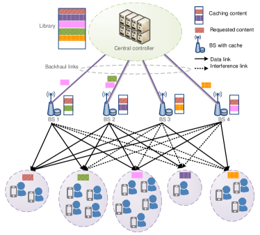
We consider a downlink multicast network consisting of single-antenna MUs cooperatively served by multi-antenna BSs, where the -th BS has antennas. Each BS is equipped with a cache storage and connected to the central controller via a capacity-limited backhaul link. The central controller has access to the whole data library containing pieces of equal-size content objects. Let , and denote the sets of BSs, MUs and content objects, respectively. At the beginning of each interval, each MU makes a content request which follows a content popularity distribution. The MUs requesting the same content are grouped together and served by a cluster of BSs using multicast transmission. During each interval, the number of multicast groups is (), and the set of groups is denoted as . The set of MUs in group is denoted as . Since each MU is assumed to request one piece of content during an interval, we have , for , and . When BS caches the content requested by group , BS can directly transmit the local content to group . Otherwise, the uncached content has to be retrieved from the central controller to BS via the corresponding backhaul link and then transmitted to group . The system model is illustrated in Fig. 1.
The propagation channel from the -th BS to the -th MU is denoted as , and the transmit beamforming vector from the -th BS to the multicast group is denoted as . The transmit signal at the -th BS is given by
| (1) |
where stands for the encoded information symbol for the multicast group with . The received signal at the MU is given by
| (2) |
where is the additive Gaussian noise at the -th MU. Assume that all MUs adopt single user detection and thus treat interference as noise. The signal-to-interference-plus-noise ratio (SINR) at MU is given by
| (3) |
where with , represents the channel vector from all the BSs to the -th MU, and represents the beamforming vector from all the BSs to group . Let denote the aggregate beamforming vector with as the beamforming vector from the -th BS to all multicast groups, i.e.,
| (4) |
To keep the analysis simple, we assume that each BS has the same number of antennas, i.e., . Define the target SINR vector as , where stands for the lowest received SINR threshold for the users in group . In order to decode the message successfully, any user , should satisfy the following QoS constraint
| (5) |
Denote the maximum transmit power of the -th BS as , and transmit power constraints are given by
| (6) |
II-B Caching and Backhaul Models
Caching networks operate in two phases, i.e., the prefetching phase and the delivery phase. In the prefetching phase, BSs fetch some contents from the file library of the central controller and store them at local caches, which usually happens during off-peak time. In the delivery phase (usually the busy hours), MUs may request arbitrary content in the file library. Since some desired contents have already been cached locally in the prefetching phase, only the rest of the requested content objects need to be delivered to BSs via backhaul links.
Define a caching matrix , where means that the -th content is cached at the -th BS. Assume that MUs in group request content , and means that the content requested by MUs in group is cached at the -th BS. The transmit association status matrix is denoted as , where means that the -th BS serves group and means the opposite. Let denote the backhaul data assignment matrix, where means that the content requested by the -th user group will be assigned to the -th BS via its backhaul link. It is not difficult to obtain that
| (7) |
Therefore, only when and , it will spawn backhaul traffic to retrieve the requested content, i.e., , and otherwise we have .
For ease of discussion, we consider fixed and feasible target SINR requirements as in [19]. The transmission data rate for group is given by where is the available bandwidth. The data rate (i.e., the traffic load) of backhaul link is then given by
| (8) |
Since the capacity of each backhaul link is limited, we consider the following backhaul capacity constraints
| (9) |
II-C Power Consumption Model
We focus on the network power consumption of the delivery phase, for which the signal processing and optimization are much more challenging than the prefetching phase. Owing to the advances in caching hardwares [11], caches have been made very energy-efficient. Moreover, once the cache placement is finished in the prefetching phase, it will remain unchanged for a period of time, e.g., several days or weeks, since the file popularity evolves slowly, while user requests happen much more frequently. Therefore, the frequent reuse of cached contents can save considerable backhaul power consumption, which makes the power consumption in the prefetching phase negligible. Also, the cache placement is usually conducted during off-peak hours when the electricity resource is abundant and with a low price. Therefore, we focus on the network power consumption for the delivery phase, and omit the power consumption for caching. The main components of network power consumption, i.e, BS power consumption and backhaul power consumption, will be modeled as follows.
II-C1 BS Power Consumption Model
We adopt the empirical linear model [25] to describe the power consumption of the -th BS:
| (10) |
where () stands for the active (sleep) mode power consumption, represents the slope of the load-dependent power consumption, and is the BS transmit power, i.e., . Although a BS’s power consumption can be arbitrarily close to zero Watt in the deepest sleep level, it may cause an undesirable long delay to wake up the BS from this low power mode [26]. In practice, when a BS has no transmission tasks, a less deep sleep mode is usually adopted, where only some well-selected parts of the hardware may be inactivated, in order to fasten the activation process. As a result, it is typical to have . For instance, according to the survey on BS power consumption [25], for a 2-antenna pico-BS, the typical values are , and . Let and denote the sets of active BSs and inactive BSs, respectively. Then, the total BS power consumption is given by
| (11) |
Based on the BS power consumption model, we conclude that it is essential to put BSs into sleep mode whenever possible in order to save the power consumption.
II-C2 Backhaul Transport Power Consumption Model
The total backhaul transport power consumption is given by
| (12) |
where is the power consumption of the backhaul link corresponding to BS . Similar to the BS power consumption model, we need to consider both active and sleep modes for backhaul links. The power consumption of an active backhaul link turns out to be traffic-dependent [43]. Therefore, the backhaul transport power consumption is expressed as
| (13) |
where denotes the maximum data rate (i.e., capacity) of the backhaul link, represents the backhaul power consumption when supporting the maximum data rate, and is the backhaul transport energy coefficient. For a backhaul link, typical values are , . The typical value for is around for microwave backhaul link [43], and around for copper DSL [4]. The power consumption of all backhaul links can be calculated as
| (14) |
Combining formula (8), (11) and (14), we have the total network power consumption as
| (15) | ||||
| (16) |
where
| (17) |
is the difference of static state power consumption between active and sleep modes for BS and its corresponding backhaul link, and is named as the relative power consumption for simplification. As a matter of fact, usually we have and , and thus . Let denote the backhaul power consumption for BS for serving user group . Since constant terms will not influence the optimization design, we can equivalently minimize the re-defined network power consumption instead of (16):
| (18) |
which consists of BS transmit power consumption, traffic-dependent backhaul power consumption, and relative power consumption of active BSs and corresponding backhaul links.
III Problem Formulation and Analysis
In this section, we will first formulate the network power minimization problem, which will then be analyzed and reformulated to reveal the layered group sparsity structure in the optimization variables. Based on (18), there are three strategies minimizing the network power consumption: i) to reduce the relative power consumption by switching off as many BSs and corresponding backhaul links as possible; ii) to reduce the transmit power consumption of BSs with coordinated beamforming by having more active BSs; and iii) to reduce the traffic-dependent backhaul power consumption by minimizing backhaul delivery of uncached content. Obviously, these strategies cannot be achieved at the same time. Hence, the network power consumption minimization problem will be a joint design across BS selection, backhaul data assignment and coordinated transmit beamforming.
III-A Problem Formulation
In this work, we assume that perfect channel state information (CSI) , cache placement , and overall user requests are known a priori at the central controller. Considering MU QoS requirements, BS transmit power constraints and per-BS backhaul capacity constraints, we formulate the network power consumption minimization problem as a joint active BS selection, backhaul data assignment and transmit beamforming design problem:
| (19) | ||||
| subject to | ||||
In the following subsection, we will analyze problem , which will motivate us to reformulate it for developing low-complexity algorithms.
III-B Problem Analysis
In this subsection, we will identify the main challenges of the network power minimization problem . We first consider the case with a given active BS set and a given backhaul data assignment matrix , resulting in a transmit power minimization problem given by
| (20) | ||||
| subject to |
which is a multicast beamforming problem as discussed in [44].
The above analysis implies that once the optimal and are identified, the solution can be determined by solving problem . Thus, problem can be solved by searching over all the possible active BS sets and all possible ’s, i.e.,
| (21) |
where is the minimum number of active BSs to meet the QoS constraints, and is determined by
| (22) |
where is the optimal value of problem and is the cardinality of set . Since the number of subsets of size is and we need to search over possible ’s for each subset , the complexity of the overall search procedure will grow exponentially with , which makes this approach unscalable. Therefore, the key to solve the problem is to effectively determine and . This problem needs to be reformulated to develop more efficient algorithms.
III-C Layered Group Sparse Beamforming Formulation
In the following, we will reformulate the original problem. First, let us present several key observations, aiming at exploiting the unique structure of the problem, which will help us address the main challenges. The original objective can be decomposed into three parts, i.e.,
| (23) |
where is the BS transmit power consumption, is the relative power consumption, and is the backhaul power consumption. We will show that and can be expressed as functions of the aggregate beamforming vector , which are able to indicate the group sparsity of at different layers.
III-C1 BS-layer Group Sparsity of
All the coefficients in a given vector form a BS-layer group and can be considered as a group sparsity measure of . When the -th BS is switched off, all the coefficients in vector will be set to zero, i.e., . It is possible that multiple BSs can be switched off and the corresponding beamformers will be set to zero, which means that has a BS-layer group sparsity structure. It is observed that if , then we have , and if , we have . Therefore, for a given beamformer , the relative power consumption can be rewritten as
| (24) |
III-C2 Data Assignment-layer Group Sparsity of
The backhaul data assignment matrix can be fully specified with the knowledge of the beamformer as
| (25) |
From (25), we observe that for a given user group , when BS does not serve it, i.e., , there is no need to assign the content requested by this user group to BS , and will be set to zero; when the content requested by user group happens to be cached at BS , i.e., , regardless of whether BS serves this user group or not, there is no need to assign the content requested by this user group to BS , and hence will always be set to zero. It is likely that we can reduce the number of backhaul data assignments and the corresponding values will be set to zero, from which we can infer that the backhaul data assignment matrix has a sparsity structure. In addition, we observe
| (26) |
which means that minimizing can imply the minimization of . All the coefficients in a given vector form a group and can be considered as another group sparsity measure of . Since this measure is related to the backhaul data assignment, it can be regarded to represent the “data assignment-layer” group sparsity. Hence, the backhaul power consumption can be rewritten as
| (27) |
For a given BS , are non-overlapping subgroups of , and is a sufficient condition for . As a result, can be simplified as
| (28) |
Based on the above discussions, the network power minimization problem can be equivalently reformulated as the following group sparse beamforming problem:
| (29) | ||||
| subject to | ||||
The equivalence between problem and problem means that if is a solution to problem , then with and is a solution to problem , and vice versa.
The incorporation of two group-sparsity measures in our problem formulation generalizes those in previous works [33, 19] which considered only one group-sparsity measure. Notice that all these group sparse beamforming problems can be unified in the following generalized group structured optimization problem:
| (30) | ||||
| subject to |
where is a smoothed convex function, and are regularization parameters for groups at different layers. When take variant combinations, the model falls into different problems, as shown in Table I.
| Parameters | Problem | Algorithm |
|---|---|---|
| Transmit power minimization | Coordinated beamforming [21] | |
| BS selection | Group sparse beamforming [23, 33, 19] | |
| Backhaul data assignment | ||
| BS selection + backhaul data assignment | Proposed layered group sparse beamforming |
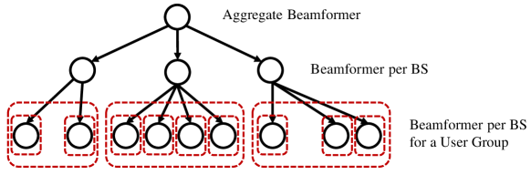
In our formulation, we have , which means that we incorporate multiple sparsity-inducing regularizers into the objective function, and therefore enable joint optimization of BS selection and backhaul data assignment, which generalizes the previous works. Specifically, the entries of are partitioned into different groups at two layers: i) the BS-layer where the beamforming coefficients sent from each BS form a group (the number of groups of this layer is ), and ii) the data assignment-layer where the beamforming coefficients associated with one BS and one user group are considered as a group (the number of groups of this layer is ). Furthermore, the previous works [33, 19] failed to take the per-BS backhaul capacity constraints into consideration, which restricts their practical applications. In order to solve problem , we are confronted with several unique challenges which are highlighted as follows.
III-C3 Combinatorial Objective Function
There are two indicator functions in , acting as two group-sparsity measures inducing group sparsity at different layers to the problem. Moreover, the variables in the two group-sparsity measures are non-separable. All the existing group sparse beamforming methods [33, 24, 34, 19] can only deal with one group-sparsity measure and are not applicable to our problem.
III-C4 Non-convex Quadratic QoS Constraints
The non-convex quadratic QoS constraints are yielded by the physical-layer multicast beamforming problem. Consider problem as an example. On one hand, a ready approach to deal with these constraints is to apply a semidefinite relaxation (SDR) technique [44], and relax problem into a semidefinite programming (SDP) problem by removing the rank-one constraints, at the price of lifting the variables to higher dimensions. On the other hand, the non-convex quadratic QoS constraints can also be rewritten into the DC form [19]. Compared to the SDP transformation, the DC transformation will not incur loss of optimality since it does not involve rank-one constraints. Moreover, the number of variables in the SDP transformation is almost the square of that in problem , while the number of variables in the DC transformation nearly remains the same as that in problem .
III-C5 Non-convex per-BS Backhaul Capacity Constraints
Besides the aforementioned difficulties, the discrete indicator function in per-BS backhaul capacity constraint, which characterizes whether BS serves user group , makes the problem much more challenging. A key observation is that the indicator function can be equivalently expressed as an -norm of a scalar. The -norm stands for the number of nonzero entries in a vector, and reduces to an indicator function in the scalar case. By using ideas from previous literature [24], we may further approximate the non-convex -norm by a convex reweighted -norm.
Based on the challenges identified above, we will propose a low-complexity algorithm to solve the problem efficiently based on the formulation in the following section.
IV Layered Group Sparse Beamforming Framework
In this section, based on the formulation , we will develop a low-complexity algorithm. The main motivation is to induce group sparsity in the aggregate beamformer at both the BS-layer and the data assignment-layer to minimize the total network power consumption. The proposed framework has three stages, as shown in Fig. 2.
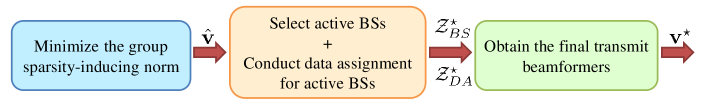
At the first stage, we solve a reweighted group sparsity-inducing norm minimization problem, so as to induce a group sparsity structure in the aggregate beamformer. Then, in the second stage, based on the approximately sparse beamformer obtained from the first stage, we will conduct a two-layer iterative search procedure, which can efficiently identify the active BSs and backhaul data assignment, respectively. In the last stage, with the knowledge of the active BS set and backhaul data assignment, coordinated multicast beamforming will be adopted to obtain the final beamformers. The details will be presented in the following subsections.
IV-A Preliminaries and Motivation of LGSBF framework
In order to induce group sparsity in the aggregate beamformer , we first replace the indicator functions by -norm, which is thereafter relaxed into the mixed -norm () [45]. The mixed -norm and -norm are two commonly used norms (also called regularizers) for inducing group sparsity. The mixed -norm is the most common choice and known as the group least-absolute selection and shrinkage operator (group Lasso). In this study, we also adopt , and obtain a convex approximation for the objective as
| (31) |
where , and , are positive weights. Compared with existing sparse beamforming methods dealing with only one sparsity-inducing regularizer [34, 19], the problem is even more complicated since its objective function has incorporated two sparsity-inducing regularizers. The multiple sparsity-inducing regularizers indicate that the solution has a layered group sparse pattern, based on which we name the proposed framework as a layered group sparse beamforming (LGSBF) framework. Moreover, in our problem, we are facing noncovex constraints as discussed in Section III, which add more challenges.
IV-B Stage I: Group Structured Sparsity Inducing Norm Minimization
In this subsection, we propose a convex relaxation for problem . To start with, we adopt the DC transformation to deal with the non-convex quadratic QoS constraints, which are rewritten as
| (32) |
Then, we need to address the indicator functions in both the objective function and backhaul capacity constraints. As stated in (31), we use the convex surrogate for the objective function by employing the mixed -norm to approximate the nonconvex -norm. The indicator function can be equivalently expressed as an -norm of another scalar instead of , i.e.,
| (33) |
which allows us to extend the mixed -norm approximation. In order to further enhance sparsity, we employ an iterative re-weighted -minimization, inspired by the reweighted -minimization proposed in [46]. The surrogate objective is rewritten as
| (34) |
and the problem is reformulated as
| (35) | ||||
| subject to | ||||
where is a weight associated with the -th BS, and is a weight associated with the -th BS and the -th user group. Similar to [46], we develop the iterative weight update rules as
| (36) |
with and obtained from the previous iteration and a small constant parameter . Since the beamformer (or ) with a lower transmit power usually has less impact, its transmit power should be encouraged to be further reduced, and eventually forced to zero, in order to switch off this BS (and its backhaul data delivery). Consequently, we are motivated to design weight updating rules (36) where and are inversely proportional to the transmit power. The small parameter is introduced to provide stability, and to ensure that a zero-valued component (or ) does not strictly prohibit a nonzero estimate at the next step. Similar heuristic updating rules were also adopted in [24].
It is observed that problem has a convex objective function, as well as DC constraints and convex constraints, and thus falls into the category of the general DC programming problems which take the following form:
| (37) | ||||
| subject to |
where and , for , are convex functions. The concave-convex procedure (CCCP) [47] has been developed to reach a local minimum of DC programming problems with a guaranteed convergence, where can be updated by solving the convex subproblem:
| (38) | ||||
| subject to |
where
| (39) |
for all . To be specific, for problem , the subproblem in the -th iteration of the CCCP takes the following form:
| (40) | ||||
| subject to | (40a) | |||
where the coefficients
| (43) |
are updated with the solution obtained in the previous iteration. In the -th iteration, we obtain the solution by solving problem (40). Problem (40) is a convex quadratically constrained quadratic program (QCQP), which can be regarded as a special case of a second-order cone program (SOCP) and can be readily solved by interior-point methods with complexity as [48]. To solve our problem efficiently, we need to carefully choose an initial feasible point for the CCCP algorithm. Therefore, an initialization step is proposed by solving a transmit power minimization problem with SDR technique [44], i.e.,
| (44) | ||||
| subject to | ||||
where we define two matrices and , to lift the quadratic constraints into higher dimensions. Moreover, we define a set of selective matrices , with as a diagonal matrix. All are rank-one constrained. If the solution are all rank-one, the feasible beamformers obtained by applying the eigenvalue decomposition (EVD) on can be directly employed as the initial feasible point for the CCCP algorithm. If the solutions are not rank-one, are obtained through randomizing and scaling. If problem is infeasible, the original problem is infeasible and the optimization has to terminate.
After solving problem , we will obtain the sparse beamforming vector as the output of the first stage, as shown in Fig. 2. The algorithm solving the group sparsity-inducing norm minimization problem for the first stage is presented as Algorithm 1, which will converge to local minima or saddle points of problem [47, 49], if it is feasible.
Step 1: Find an initial feasible point by solving problem ;
Step 2: Initialize, , and set the iteration counter as ;
Step 3: Repeat
Step 4: Until stopping criterion is met and obtain the beamformer ;
End
IV-C Stage II: Iterative Search Procedure
Inducing the sparsity structure in the solution is critical to problem . As illustrated in Fig. 3, the layered group sparse pattern can be mapped to a hierarchy tree.
Generally, the solution obtained from Stage I is not strictly sparse, and thus we propose to trim the entries of to obtain the group sparse solution. Although backhaul capacity constraints can help us filter some sparsity patterns (i.e, prune some nodes in the hierarchy tree), finding the optimal sparsity pattern in brings about high computational complexity. In this subsection, we develop an efficient search procedure to identify active BSs and backhaul data assignment.
IV-C1 BS Ordering and Selection
With the knowledge of the input , the next step is to determine the active BS set. After giving proper priorities to BSs, we can obtain an ordering list to switch them off. Previous works have considered different ways to calculate the priorities. For example, Mehanna et al. [50] directly mapped the group-sparsity obtained by the group-sparsity inducing norm minimization to their application, i.e., the transmit antennas with smaller coefficients in the group were determined to be turned off with a higher priority. Following this idea, in our setting, the priorities might be given as which implies that the BS with a lower transmit beamforming gain should be encouraged to be switched off. However, such a direct mapping might bring performance degradation, as shown in [33]. To get a better performance, it is essential to consider not only the transmit beamforming gain but also other key system parameters indicating the impact of the BSs on the network performance. Similar to the one employed in [33], to assign priorities to BSs, we propose the following ordering criteria that incorporates channel power gain, BS power amplifier efficiency, relative power consumption, backhaul power consumption, caching status and beamforming gain, that is,
| (45) |
where is the channel gain from the -th BS to all MUs. The BS with a higher priority (i.e., smaller ) will be switched off before the one with a lower priority (i.e., larger ). This ordering criteria implies that the BS with a lower channel power gain, lower BS power amplifier efficiency (i.e., higher ), higher relative transport link power consumption, higher backhaul power consumption and lower cache hit ratio should have a higher priority to be switched off.
Once BS is decided to be switched off, all its corresponding beamforming coefficients will be set to zero, i.e, . Based on the ordering criteria rule, we sort the coefficients in ascending order. Each time a BS is decided to be switched off, the inactive BS set will be updated and we check a feasibility problem
| (46) | ||||
| subject to | ||||
which is a DC programming, and can be solved by the CCCP algorithm.
IV-C2 Backhaul Data Assignment for Active BSs
If problem is feasible, the next question is to determine the backhaul data assignment for the active BSs in order to further reduce the power consumption. Similar to the design idea for (45), we calculate priorities of backhaul data assignment for the active BSs by taking the aforementioned key system parameters into consideration. Consequently, we propose the following ordering criteria to determine which backhaul data assignment should be turned off, i.e.,
| (47) |
where is the channel gain from the -th BS to the MUs in the -th user group. Based on the ordering criteria, we delete a piece of data assignment each time and update the inactive data assignment set . With and , the subproblem that we need to solve takes the following form:
| (48) | ||||
| subject to | ||||
which is also a DC program, and can be solved by the CCCP algorithm.
Realizing that switching off as many BSs as possible may not result in a minimum total network power consumption, we are motivated to adopt a conservative strategy to determine the final active BS set and backhaul data assignment. To obtain the minimum network power consumption, we iteratively search over all possible and , and record the corresponding network power. By comparing all the recorded values, we can determine that corresponds to the minimal network power consumption. Overall, the iterative search method can be accomplished via solving no more than DC problems.
IV-D Stage III: Obtain Transmit Beamformers
With the obtained inactive BS set and inactive data assignment set , we can obtain the final beamforming vector by solving the following problem:
| (49) | ||||
| subject to | ||||
which is also a DC program. In principle, problem (49) can be globally solved via the branch-and bound algorithm by extending the method developed in [51]. Such global optimization algorithms have high computational complexity, and cannot be applied in dense networks. Therefore, the CCCP algorithm is adopted to efficiently obtain a local optimal solution. The overall iterative LGSBF algorithm is summarized in Algorithm 2.
Step 1: Solve problem by applying Algorithm 1: if it is infeasible, go to End; otherwise, obtain ;
Step 2: Calculate the ordering criterion (45), and sort the values in the ascending order ;
Step 3: Initialize , and ;
Step 4: Solve the optimization problem
-
1.
If is feasible,
-
(a)
Calculate the ordering criterion (47), and sort the values in the ascending order ;
-
(b)
Initialize , and ;
-
(c)
Repeat Solve the optimization problem , update the set and ;
-
(d)
Until infeasible, obtain ;
-
(e)
Update the set and , go to Step 4;
-
(a)
-
2.
If is infeasible, obtain , go to Step 5;
Step 5: Obtain the optimal inactive BS set and inactive data assignment set by solving ;
Step 6: Obtain beamformers by solving problem ;
End
Note that the proposed approach provides a general framework for a multi-layer GSBF problem, where various group sparsity-inducing algorithms, e.g., the smoothed -minimization [34], can be applied in Stage I.
IV-E Complexity and Convergence Analysis
It has been shown that for the iterative search procedure, the number of general DC problems to be solved is no more than . To obtain a local optimal solution for general DC programs, at each iteration of the CCCP-based algorithm, we need to solve a convex QCQP (or equivalently SOCP) problem with a complexity of by interior-point methods, which constitutes the main computational complexity of the proposed LGSBF algorithm. For large-scale networks, other approaches for solving large-sized SOCPs, e.g., the alternating direction method of multipliers (ADMM) method [52], need to be explored. For unconstrained DC programs with differentiable objectives, it could converge superlinearly [49], while the convergence rate of general DC programs is still an open problem.
V Simulation results
In this section, we simulate the performance of the proposed algorithm. We consider a hexagonal multicell network, where each BS is located at the center of a hexagonal cell whose radius is set to be , and MUs are uniformly and independently distributed in the network, excluding an inner circle of around each BS. The channel between the -th BS and the -th user is modeled as where is the path-loss at distance , is the shadowing coefficient, is transmit antenna power gain and is the small scale fading coefficient. We adopt the standard cellular network parameters as presented in Table II.
| Parameter | Value |
|---|---|
| Transmit antenna power gain | |
| Path-loss at distance (km) | |
| Standard deviation of log-norm shadowing | |
| Small scale fading distribution | |
| Noise power spectral density | |
| Bandwidth | |
| Maximum BS transmit power | |
| Slope of the load-dependent power consumption |
The file library contains 100 pieces of content, whose popularity follows a Zipf distribution with parameter . In this popularity model, a small implies a flat popularity distribution, while a large means the opposite. BSs are assumed to have equal cache sizes. We shall briefly show the role of cache by varying the cache size and caching strategies via simulations. Herein, we consider two widely-employed heuristic caching strategies, i.e., the most popular caching (MPC) [53] and probabilistic caching (ProbC) [19, 54]. For MPC, each BS caches as many popular files as possible in accordance with the file popularity rank in the descending order. As for ProbC, each BS randomly caches files with the same probabilities as their request probabilities. Assume that the SINR requirements for different user groups are the same, i.e., .
V-A Network Power Consumption
Consider a network with BSs, each of which has two antennas, and single-antenna MUs. We set the relative power consumption as , backhaul energy coefficient as , and per-BS backhaul capacity as . Each BS has a cache size of 10 files [54], i.e., .
The proposed algorithm is compared with the following algorithms:
-
•
Coordinated beamforming (CB) algorithm: In this algorithm [42], all BSs are in the active mode and only the total BS transmit power consumption is minimized.
-
•
Sparse multicast beamforming algorithm with adaptive BS selection: This algorithm [34] develops a procedure to switch off as many BSs as possible. The non-convex smoothed -norm is adopted to replace the convex mixed -norm in the objective function. The non-convex quadratic forms of beamforming vectors in the objective function and the non-convex quadratic QoS constraints are relaxed by leveraging SDR technique. Then an iterative reweighted- algorithm is employed to solve the problem.
-
•
Sparse multicast beamforming algorithm with adaptive backhaul content assignment: In this algorithm [19], the number of backhaul content assignments is minimized. Smooth approximated functions are employed to approximate the -norm terms and a generalized CCCP algorithm is applied to solve the problem. The arctangent function is adopted since [19] shows it gives the best approximation performance.
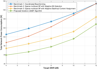
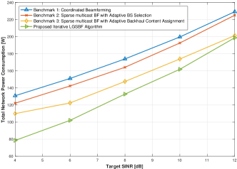
Fig. 4 demonstrates the total network power consumption with different target SINR values under MPC and ProbC, respectively. It shows that the proposed iterative LGSBF algorithm outperforms existing algorithms with both caching strategies, which confirms the effectiveness of the proposed algorithm. When the target SINR increases, it is observed that the gap between different algorithms becomes smaller, while benchmark 2 converges to CB faster than benchmark 3 and the proposed algorithm. It is because that more and more BSs need to be switched on to support the increasing QoS requirements, which decreases the benefit of active BS selection. Whereas, a careful design for backhaul content assignment can still help reduce network power consumption, since it can bring some cooperation chance for BSs and avoid unnecessary backhaul consumption at the same time.
Remark 1. The proposed algorithm achieves a better performance than those of [34] and [19] by considering a two-layer adaptive selection for both active BS and actual backhaul assignment instead of the existing one-layer approaches. This indicates that the joint adaptive decision of BS selection and backhaul content assignment can effectively reduce network power consumption for a wide range of target SINRs.
Remark 2. Comparing two caching strategies, we observe that MPC performs better than ProbC in reducing network power consumption, and the gap becomes larger when the target SINR increases. In general, MPC provides better performance than ProbC for normal network settings, and similar findings are also observed in [19].
V-B Impact of Cache Size
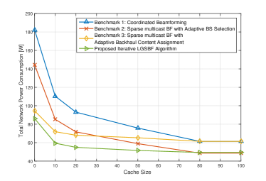
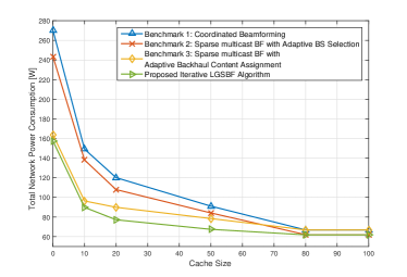
In Fig. 5(a) and Fig. 5(b), we compare the performance of the proposed algorithm with benchmarks in terms of the tradeoff between total network power consumption and per-BS cache size under target and target , respectively. Other settings are the same as those in Fig. 4. From Fig. 5, it is observed that the proposed algorithm outperforms benchmarks under different cache sizes. Moreover, the advantage of adaptive backhaul content assignment will gradually be surpassed by adaptive BS selection when the cache size increases; at a higher target SINR regime, the crosspoint will occur at a larger cache size. Besides this, the proposed algorithm achieves a better performance in a low SINR regime. It can be inferred that the increase in the cache size allows more BSs to be switched off, especially when the QoS requirement is comparatively low.
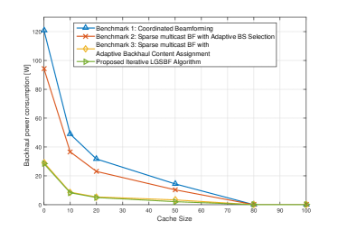
With the same network setting as in Fig. 5(a), the details of the impact of caching on the BSs and backhaul links are demonstrated in Fig. 6. This figure shows that the CB algorithm, which intends to minimize the BS transmit power consumption, has the highest backhaul power consumption. This is because all the BSs are active in the CB algorithm in order to achieve the highest beamforming gain. Moreover, by comparing Benchmark 2, Benchmark 3 and the proposed algorithm, it can be inferred that minimizing either the number of active BSs or the number of backhaul content delivery cannot be the optimal strategy to save power. Since both the backhaul power consumption and BS power consumption hold a nontrivial share, a joint adaptive BS selection, backhaul data assignment and power minimization beamforming is crucial for minimizing the total network power consumption.

V-C Impact of the Number of Mobile Users and Backhaul Energy Coefficient
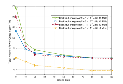
We also investigate the impact of other important network parameters, i.e., the number of MUs and backhaul energy coefficient, as shown in Fig. 7. The figure demonstrates that when the number of MUs increases, the performance gap between the zero-cache case and full-cache case becomes larger. On the other hand, Fig. 7 also shows that the performance gap between the zero-cache case and full-cache case is larger for the network with a higher backhaul energy coefficient. Actually, different backhaul energy coefficients represent different types of backhaul links: a higher backhaul energy coefficient stands for less power-efficient backhaul links, and vice versa. To enhance the performance in total network power consumption, the operators can either upgrade the backhaul links, which is expensive, or simply install cost-effective caches. From the simulation, we can infer that caches will play a more significant part in networks with higher user densities, and less power-efficient backhaul links.
VI Conclusions
In this study, we developed an effective framework to minimize the total network power consumption of cache-enabled wireless networks. The proposed LGSBF formulation generalized existing works on group sparse beamforming, for which an effective algorithm was developed. The proposed algorithm can significantly reduce the total network power consumption via a joint design of adaptive BS selection, backhaul content assignment and multicast beamforming. From the simulations, the proposed LGSBF framework was demonstrated to outperform existing algorithms by striking a balance between the BS power consumption and backhaul power consumption. Furthermore, it was shown that caching tends to play a more significant part in networks with higher user densities and less power-efficient backhaul links. For future research directions, it would be interesting to optimize the caching placement in the prefetching phase, and incorporate it when minimizing the total network power consumption. It is also important but challenging to develop more efficient distributed algorithms for practical implementation in large-scale networks.
References
- [1] Cisco Systems Inc., “Cisco visual networking index: Global mobile data traffic forecast update, 2016-2021,” White Paper, Feb. 2017.
- [2] N. Bhushan, J. Li, D. Malladi, R. Gilmore, D. Brenner, A. Damnjanovic, R. T. Sukhavasi, C. Patel, and S. Geirhofer, “Network densification: The dominant theme for wireless evolution into 5G,” IEEE Commun. Mag., vol. 52, no. 2, pp. 82–89, Feb. 2014.
- [3] D. Lee, H. Seo, B. Clerckx, E. Hardouin, D. Mazzarese, S. Nagata, and K. Sayana, “Coordinated multipoint transmission and reception in LTE-advanced: Deployment scenarios and operational challenges,” IEEE Commun. Mag., vol. 50, no. 2, pp. 148–155, Feb. 2012.
- [4] D. Schien, P. Shabajee, M. Yearworth, and C. Preist, “Modeling and assessing variability in energy consumption during the use stage of online multimedia services,” J. Ind. Ecol., vol. 17, no. 6, pp. 800–813, Dec. 2013.
- [5] X. Ge, H. Cheng, M. Guizani, and T. Han, “5G wireless backhaul networks: Challenges and research advances,” IEEE Netw., vol. 28, no. 6, pp. 6–11, Nov. 2014.
- [6] K. Shanmugam, N. Golrezaei, A. Dimakis, A. Molisch, and G. Caire, “Femtocaching: Wireless content delivery through distributed caching helpers,” IEEE Trans. Inf. Theory, vol. 59, no. 12, pp. 8402–8413, Dec. 2013.
- [7] X. Wang, A. V. Vasilakos, M. Chen, Y. Liu, and T. T. Kwon, “A survey of green mobile networks: Opportunities and challenges,” Mobile Netw. Appl., vol. 17, no. 1, pp. 4–20, 2012.
- [8] F. Richter, A. J. Fehske, P. Marsch, and G. P. Fettweis, “Traffic demand and energy efficiency in heterogeneous cellular mobile radio networks,” in Proc. IEEE Vehicular Technology Conference (VTC), Taipei, Taiwan, May 2010, pp. 1–6.
- [9] F. Zhuang and V. Lau, “Backhaul limited asymmetric cooperation for MIMO cellular networks via semidefinite relaxation,” IEEE Trans. Signal Process., vol. 62, no. 3, pp. 684–693, Feb. 2014.
- [10] S. Tombaz, P. Monti, K. Wang, A. Vastberg, M. Forzati, and J. Zander, “Impact of backhauling power consumption on the deployment of heterogeneous mobile networks,” in IEEE Global Commun. Conf. (GLOBECOM), Houston, TX, Dec. 2011, pp. 1–5.
- [11] N. Choi, K. Guan, D. C. Kilper, and G. Atkinson, “In-network caching effect on optimal energy consumption in content-centric networking,” in Proc. IEEE Int. Conf. Commun. (ICC), Ottawa, Canada, Jun. 2012, pp. 2889–2894.
- [12] N. Golrezaei, K. Shanmugam, A. G. Dimakis, A. F. Molisch, and G. Caire, “Femtocaching: Wireless video content delivery through distributed caching helpers,” in Proc. IEEE Int. Conf. Computer Commun. (INFOCOM), Orlando, FL, Mar. 2012, pp. 1107–1115.
- [13] M. A. Maddah-Ali and U. Niesen, “Cache-aided interference channels,” in Proc. IEEE Int. Symp. Inf. Theory (ISIT), Hong Kong, Jun. 2015, pp. 809–813.
- [14] ——, “Cache-aided interference channels,” arXiv preprint, Jun. 2017. [Online]. Available: http://arxiv.org/abs/1510.06121v2
- [15] J. Li, Y. Chen, Z. Lin, W. Chen, B. Vucetic, and L. Hanzo, “Distributed caching for data dissemination in the downlink of heterogeneous networks,” IEEE Trans. Commun., vol. 63, no. 10, pp. 3553–3568, Oct. 2015.
- [16] J. Liu, B. Bai, J. Zhang, and K. B. Letaief, “Content caching at the wireless network edge: A distributed algorithm via belief propagation,” in Proc. IEEE Int. Conf. Commun. (ICC), Kuala Lumpur, Malaysia, May 2016, pp. 1–6.
- [17] E. Baştug, M. Bennis, M. Kountouris, and M. Debbah, “Cache-enabled small cell networks: Modeling and tradeoffs,” EURASIP J. Wireless Commun. Netw., vol. 2015, no. 1, pp. 41–51, Feb. 2015.
- [18] A. Liu and V. K. N. Lau, “Mixed-timescale precoding and cache control in cached mimo interference network,” IEEE Trans. Signal Process., vol. 61, no. 24, pp. 6320–6332, Dec. 2013.
- [19] M. Tao, E. Chen, H. Zhou, and W. Yu, “Content-centric sparse multicast beamforming for cache-enabled cloud RAN,” IEEE Trans. Wireless Commun., vol. 15, no. 9, pp. 6118–6131, Sept. 2016.
- [20] A. Sengupta, R. Tandon, and O. Simeone, “Fog-aided wireless networks for content delivery: Fundamental latency trade-offs,” arXiv preprint, Jun. 2017. [Online]. Available: http://arxiv.org/abs/1605.01690v5
- [21] J. Zhang, R. Chen, J. G. Andrews, A. Ghosh, and R. W. Heath, “Networked MIMO with clustered linear precoding,” IEEE Trans. Wireless Commun., vol. 8, no. 4, pp. 1910–1921, Apr. 2009.
- [22] C. T. K. Ng and H. Huang, “Linear precoding in cooperative MIMO cellular networks with limited coordination clusters,” IEEE J. Select. Areas Commun., vol. 28, no. 9, pp. 1446–1454, Dec. 2010.
- [23] M. Hong, R. Sun, H. Baligh, and Z.-Q. Luo, “Joint base station clustering and beamformer design for partial coordinated transmission in heterogeneous networks,” IEEE J. Sel. Areas Commun., vol. 31, no. 2, pp. 226–240, Feb. 2013.
- [24] B. Dai and W. Yu, “Sparse beamforming and user-centric clustering for downlink cloud radio access network,” IEEE Access, vol. 2, pp. 1326–1339, Nov. 2014.
- [25] G. Auer, V. Giannini, C. Desset, I. Godor, P. Skillermark, M. Olsson, M. Imran, D. Sabella, M. Gonzalez, O. Blume, and A. Fehske, “How much energy is needed to run a wireless network?” IEEE Wireless Commun., vol. 18, no. 5, pp. 40–49, Oct. 2011.
- [26] P. Frenger, P. Moberg, J. Malmodin, Y. Jading, and I. Godor, “Reducing energy consumption in lte with cell DTX,” in IEEE Vehicular Technology Conference (VTC), May 2011, pp. 1–5.
- [27] J. Wu, S. Zhou, and Z. Niu, “Traffic-aware base station sleeping control and power matching for energy-delay tradeoffs in green cellular networks,” IEEE Trans. Wireless Commun., vol. 12, no. 8, pp. 4196–4209, Aug. 2013.
- [28] H. Yao, C. Fang, C. Qiu, C. Zhao, and Y. Liu, “A novel energy efficiency algorithm in green mobile networks with cache,” EURASIP J. Wireless Commun. Netw., vol. 2015, no. 1, pp. 139–147, May 2015.
- [29] J. Ghimire and C. Rosenberg, “Impact of limited backhaul capacity on user scheduling in heterogeneous networks,” in Proc. IEEE Wireless Commun. Networking Conf. (WCNC), Apr. 2014, pp. 2480–2485.
- [30] I. Atzeni, M. Maso, I. . Ghamnia, M. Debbah, and E. Baştug, “Flexible cache-aided networks with backhauling,” in Proc. IEEE Int. Workshop Signal Process. Advances in Wireless Commun. (SPAWC), Sapporo, Japan, Jul. 2017.
- [31] K. Poularakis, G. Iosifidis, V. Sourlas, and L. Tassiulas, “Exploiting caching and multicast for 5G wireless networks,” IEEE Trans. Wireless Commun., vol. 15, no. 4, pp. 2995–3007, Apr. 2016.
- [32] X. Peng, J.-C. Shen, J. Zhang, and K. B. Letaief, “Joint data assignment and beamforming for backhaul limited caching networks,” in Proc. IEEE Int. Symp. Personal Indoor and Mobile Radio Comm. (PIMRC), Washington, DC, Sept. 2014, pp. 1370–1374.
- [33] Y. Shi, J. Zhang, and K. B. Letaief, “Group sparse beamforming for green cloud-RAN,” IEEE Trans. Wireless Commun., vol. 13, no. 5, pp. 2809–2823, May 2014.
- [34] Y. Shi, J. Cheng, J. Zhang, B. Bai, W. Chen, and K. B. Letaief, “Smoothed -minimization for green Cloud-RAN with user admission control,” IEEE J. Sel. Areas Commun., vol. 34, no. 4, pp. 1022–1036, Apr. 2016.
- [35] D. L. Donoho, “Compressed sensing,” IEEE Trans. Inf. Theory, vol. 52, no. 4, pp. 1289–1306, Apr. 2006.
- [36] E. J. Candes and T. Tao, “Near-optimal signal recovery from random projections: Universal encoding strategies?” IEEE Trans. Inf. Theory, vol. 52, no. 12, pp. 5406–5425, Dec. 2006.
- [37] M. Yuan and Y. Lin, “Model selection and estimation in regression with grouped variables,” J. R. Statist. Soc. B, vol. 68, pp. 49–67, 2006.
- [38] L. Jacob, G. Obozinski, and J.-P. Vert, “Group lasso with overlap and graph lasso,” in Proc. Int. Conf. Machine Learning (ICML), 2009, pp. 433–440.
- [39] J. Wang and J. Ye, “Two-layer feature reduction for sparse-group lasso via decomposition of convex sets,” Neural Inf. Process. Syst., pp. 2132–2140, 2014.
- [40] S. Gao, L. T. Chia, and I. W. H. Tsang, “Multi-layer group sparse coding-for concurrent image classification and annotation,” in Proc. IEEE Conf. Computer Vision and Pattern Recognition (CVPR), Jun. 2011, pp. 2809–2816.
- [41] Y.-F. Liu, Y.-H. Dai, and S. Ma, “Joint power and admission control: Non-convex approximation and an effective polynomial time deflation approach,” IEEE Trans. Signal Process., vol. 63, no. 14, pp. 3641–3656, Jul. 2015.
- [42] H. Dahrouj and W. Yu, “Coordinated beamforming for the multicell multi-antenna wireless system,” IEEE Trans. Wireless Commun., vol. 9, no. 5, pp. 1748–1759, May 2010.
- [43] A. Fehske, P. Marsch, and G. Fettweis, “Bit per joule efficiency of cooperating base stations in cellular networks,” in Proc. IEEE Global Commun. Conf. (GLOBECOM) Workshop, Miami, FL, Dec. 2010, pp. 1406–1411.
- [44] N. Sidiropoulos, T. Davidson, and Z.-Q. Luo, “Transmit beamforming for physical-layer multicasting,” IEEE Trans. Signal Process., vol. 54, no. 6, pp. 2239–2251, Jun. 2006.
- [45] F. Bach, R. Jenatton, J. Mairal, and G. Obozinski, “Optimization with sparsity-inducing penalties,” Found. Trends Mach. Learn., vol. 4, no. 1, pp. 1–106, Jan. 2012.
- [46] E. J. Candes, M. B. Wakin, and S. P. Boyd, “Enhancing sparsity by reweighted minimization,” J. Fourier Anal. Appl., vol. 14, no. 5, pp. 877–905, Dec. 2008.
- [47] A. Yuille and A. Rangarajan, “The concave-convex procedure,” Neural Computation, vol. 15, no. 4, pp. 915–936, Apr. 2003.
- [48] S. P. Boyd and L. Vandenberghe, Convex Optimization. Cambridge University Press, 2004.
- [49] G. R. Lanckriet and B. K. Sriperumbudur, “On the convergence of the concave-convex procedure,” Neural Inf. Process. Syst., pp. 1759–1767, 2009.
- [50] O. Mehanna, N. D. Sidiropoulos, and G. B. Giannakis, “Joint multicast beamforming and antenna selection,” IEEE Trans. Signal Process., vol. 61, no. 10, pp. 2660–2674, May 2013.
- [51] C. Lu and Y.-F. Liu, “An efficient global algorithm for single-group multicast beamforming,” IEEE Trans. Signal Process., vol. 65, no. 14, pp. 3761–3774, Jul. 2017.
- [52] S. Boyd, N. Parikh, E. Chu, B. Peleato, and J. Eckstein, “Distributed optimization and statistical learning via the alternating direction method of multipliers,” Foundations Trends Mach. Learning, vol. 3, pp. 1–122, Jul. 2011.
- [53] H. Ahlehagh and S. Dey, “Video-aware scheduling and caching in the radio access network,” IEEE/ACM Trans. Netw., vol. 22, no. 5, pp. 1444–1462, Oct. 2014.
- [54] C. Bernardini, T. Silverston, and O. Festor, “A comparison of caching strategies for content centric networking,” in Proc. Global Commun. Conf. (GLOBECOM), San Diego, CA, Dec. 2015, pp. 1–6.