Probably approximate Bayesian computation: nonasymptotic convergence of ABC under mispecification

Abstract

Approximate Bayesian computation (ABC) is a widely used inference method in Bayesian statistics to bypass the point-wise computation of the likelihood. In this paper we develop theoretical bounds for the distance between the statistics used in ABC. We show that some versions of ABC are inherently robust to mispecification. The bounds are given in the form of oracle inequalities for a finite sample size. The dependence on the dimension of the parameter space and the number of statistics is made explicit. The results are shown to be amenable to oracle inequalities in parameter space. We apply our theoretical results to given prior distributions and data generating processes, including a non-parametric regression model. In a second part of the paper, we propose a sequential Monte Carlo (SMC) to sample from the pseudo-posterior, improving upon the state of the art samplers.

1 Introduction

A wide range of statistical applications involve models where the likelihood is not available in closed form. One typical case is when the likelihood is expressed as a multidimensional integral, as in state space models or models with high dimensional latent variables. Another well studied case appears when the normalizing constant of the likelihood is unknown, that is, the likelihood $\pi_{\theta}$ is written as $\pi_{\theta}(x)=\ell_{\theta}(x)/Z_{\theta}$, with unknown $Z_{\theta}$. More generally we consider in this paper models with hard to compute likelihoods that are relatively easy to sample from. We refer the reader to Marin et al. (2012) for further motivation for this framework.

The goal of Approximate Bayesian Computation (ABC) is to perform statistical inference in the case where the likelihood cannot be evaluated point-wise. This algorithm has found success amongst applied statisticians in fields as diverse as population genetics (Beaumont et al. (2002)), astronomy (Cameron and Pettitt (2012)), computer vision (Mansinghka et al. (2013)) etc. The general idea is to use auxiliary samples from the model for different values of the parameter and compare them with the observed variables. More precisely for a sequence of observations $(Y_{i})_{i=1}^{n}$, and a vector of summary statistics $S$, ABC can be formulated as sampling from the joint distribution

$$\pi_{h}^{abc}\left(d\theta,dX^{n}|Y^{n}\right)=\frac{K_{h}\left\{d\left(S(X^{n}),S(Y^{n})\right)\right\}\pi_{\theta}(dX^{n})\pi(d\theta)}{\int\int K_{h}\left\{d\left(S(X^{n}),S(Y^{n})\right)\right\}\pi_{\theta}(dX^{n})\pi(d\theta)},$$ (1)

where $K_{h}$ is a kernel function with window $h$, and $d$ is a distance between summary statistics. Inference in parameter space is obtained by integrating in in $X$. The intuition is to sample $\theta$ in the parameter space and an auxiliary sample $(X_{i})_{i=1}^{n}$ according to the model, such that the $(X_{i})_{i=1}^{n}$ are “close” to the observation. The kernel function enforces the closeness between the simulated data and the observations. Several kernels are proposed in practice, however two are widely used: the uniform kernel $\textbf{1}_{d(S(X^{n}),S(Y^{n}))<h}$ (corresponding to an accept reject algorithm) and the Gaussian kernel $\frac{1}{\sqrt{h}}e^{-\frac{1}{h}d^{2}(S(X^{n}),S(Y^{n}))}$.

Several points are usually discussed in the burgeoning literature of ABC: the choice of summary statistics (Fearnhead and Prangle (2012); Marin et al. (2014)), convergence of the Monte Carlo algorithm as $h$ goes to $0$ (e.g. Barber et al. (2015)) and statistical properties of the pseudo-posterior (Li and Fearnhead (2015); Frazier et al. (2016)). We focus in this paper on the latter point, the statistics are considered fixed and we let the window $h$ go to $0$ only as a function of the sample size. Taking this approach rather than trying to let $h$ go to zero with the size of the Monte Carlo sample allows an appropriate treatment of the bias introduced by ABC.

In general the validity of the pseudo-posterior is given intuitively by saying for $h\rightarrow 0$ the pseudo-posterior “should” converge to the “ideal” one (Bayesian posterior). Relatively few papers consider the statistical error induced by using distribution (1), and its rate of convergence. Notable exceptions are given in Frazier et al. (2016) in the uniform kernel case and Li and Fearnhead (2015) under moment conditions on the kernel. The former studies posterior consistency and its concentration rate as $n\rightarrow\infty$. The latter gives a central limit theorem for the posterior mean of ABC. Both papers study asymptotic convergence for models that are well specified. We can also mention the recent paper of Bernton et al. (2017) where some results in Wasserstein distance for mispecified models are adapted from Frazier et al. (2016). We also mention that since the first submission of our paper Frazier2017 proposed an extention of Frazier et al. (2016) to the misspecified case. The paper proposes an asymptotic analysis of the ABC error under misspecification. The conclusion on the robustness of ABC and the choice of the window parameter are similar. The main differences lies in the choice of the kernel $K_{h}$ (with empirical improvement), the ability to give non asymptotic results and to deal with high dimension parameters.

The form of the ABC pseudo-posterior suggests that it should allow some degree of mispecification, in a spirit similar to generalized posteriors (e.g. Zhang et al. (2006)). We call generalized posterior, for $\lambda>0$, a measure of the form

$$\pi_{\lambda}^{gen}\left(d\theta|Y^{n}\right)\propto\left\{\pi_{\theta}\left(Y^{n}\right)\right\}^{\lambda}\pi(d\theta).$$

The case $\lambda=1$ corresponds to the usual Bayesian posterior distribution. The case where $\lambda<1$ is used to deal with misspecification in Zhang et al. (2006) and Grünwald and van Ommen (2014). This works intuitively by assigning less weight to the likelihood part. In this spirit ABC seems to be built for the same kind of robustness. Similarly allowing for a bigger window (or one converging less quickly) allows for some robustness in the approach. In this paper we propose studying the convergence of the pseudo-posterior in the case where the true distribution of the sample lies outside the statistician’s model. We rely on concentration inequalities for the distance under general distributions. Bounds are given in deviation using PAC-Bayesian analysis (e.g. Catoni (2007)).

Our results will rely on the use of an exponential kernel in equation (1). This also has some computational advantages as compared to a uniform kernel. It allows to build a smooth sequence of distribution indexed by the inverse window parameter. We will propose a new Sequential Monte Carlo (SMC) algorithm to efficiently explore this sequence. We build a fully adaptive version of the algorithm of Del Moral et al. (2012) .

In the next section we define the framework that we will be using in the paper. In Section 3 we give oracle inequalities on the distance between the expected statistics. We also give some bounds on the parameters themselves under additional assumptions. In Section 3.2 we take a brief detour to develop empirical bounds. Those results can be used in practice to bound the generalization error (expected distance). We use those bounds to develop an estimator that chooses automatically the bandwidth parameter (Section 3.3). Section 4 is devoted to some application of the bounds to different priors and models.

Finally in Section 5 we build upon the sequential Monte Carlo sampler of Del Moral et al. (2012) to give an efficient way to sample from the joint pseudo-posterior. The algorithm is applied to a toy example in a numerical section (Section 6). The proofs are deferred to Section 7.

Notation

In the following we will use operator notation i.e. for a finite measure $\nu$ we write for any $f\in L^{1}(\nu)$ the expectation $\nu(f):=\int f(x)\nu(dx).$ The support of measure $\nu$ is denoted $\text{supp}(\nu)$, and vectors $Y_{n}^{m}:=(Y_{n},\cdots,Y_{m})$ for any $n<m$, we will drop the subscript when the vector starts at $1$; we also use $n:m:=\left(n,\cdots,m\right)$. For some set $A$ we write $\mathcal{M}_{1}^{+}(A)$ the set of probability measures on $A$, the $\sigma$-algebra is given by context. We use $\wedge$ and $\vee$ for the $\inf$ and $\sup$ respectively and $v_{n}\asymp r_{n}$ for two sequences such that $v_{n}/r_{n}=\mathcal{O}(1)$. The notation $\sup_{\pi}$ for $\pi\in\mathcal{M}_{+}^{1}$ is intended to mean the supremum over the support of $\pi$. Furthermore for two measures $\mu,\nu$ we write $\mu\otimes\nu$ for the product measure and $\mathcal{K}(\mu,\nu)$ for the Kullback-Leibler divergence.

2 Set up and definitions

Define a probability space $(\mathcal{Y}^{n},\mathcal{B}(\mathcal{Y}^{n}),\mathbb{P})$, we suppose that the observation $Y^{n}\in\mathcal{Y}^{n}$ is an i.i.d. collection sampled from the probability measure $\mathbb{P}$. We define a model as a collection of measures $\left(\pi_{\theta},\theta\in\Theta\right)$ on some space $\left(\mathcal{X}^{n},\mathcal{B}(\mathcal{X}^{n})\right)$ indexed by a parameter $\theta\in\Theta$. We let $(\Theta,\|.\|)$ be normed and endow $\Theta$ with the structure of a probability space $\left(\Theta,\mathcal{B}(\Theta),\pi\right)$ where $\pi$ is the prior probability.

For the moment we do not assume anything on the probability $\mathbb{P}$ other than i.i.d., furthermore this hypothesis could also be weakened. We will see that we require only some form of exponential concentration inequality for the probability, this might also be obtained for more general assumptions such as weak-dependance (e.g. Olivier et al. (2010)). To shorten formulae in the text we also define the following marginal measure $m_{X}(A):=\int_{A}\int_{\Theta}\pi(d\theta)\pi_{\theta}(dX^{n})$ for any $A\in\mathcal{B}(\mathcal{X}^{n})$. We will abuse notation and write $\pi_{\theta}\pi(dX^{n},d\theta)$ for $\pi(d\theta)\pi_{\theta}(dX^{n})$, hence $m_{X}(f)=\pi_{\theta}\pi(f)$ for any suitable function $f$ on $\mathcal{X}^{n}$.

We can now build the joint pseudo-posterior of interest. We start by defining the summary statistics. Let $(\mathcal{S},d)$ be a metric space, the summary statistics is a function $S:\mathcal{X}^{n}\cup\mathcal{Y}^{n}\mapsto\mathcal{S}$. The metric on $\mathcal{S}$ is the one we will use to compare samples in the pseudo posterior. Notice that we do not assume that the samples and the model live on the same sample space but rather that the summary statistics maps both samples to $\mathcal{S}$. In the paper we will consider cases where the observations are sampled on a bounded domain but the auxiliary sample can reach out of this set. The choice of the statistics has an impact on the quality of the approximation. The ideal case in ABC is the one where the statistics are exhaustive and the map $\theta\mapsto\pi_{\theta}(S)$ is injective (see Frazier et al. (2016)). Finding a set of statistics that correctly summarizes the distribution is of course hard, if not impossible. In particular we do not have access to the true distribution and can only hope in finding a summary statistics for our model. We will not discuss further the choice of the summary statistics as our measure of risk will itself depend on the quality of this choice.

Another degree of freedom lies in the choice of the distance. This has not been studied much in the literature. We will see that it arises in our measure of the risk associated with distribution and different dimension dependence. In the examples of Section 4 we give two possible distances for which we can give theoretical results. To simplify notations further, when it is necessary, we will write $D_{n}^{S}$ for the distance $d(S(X^{n}),S(Y^{n}))$, where $Y^{n}$ is the observed vector and $X^{n}$ is an auxiliary sample from the model. In what follows we will call $X^{n}$ the prior sample and $\left(\pi_{\theta}\right)_{\theta\in\Theta}$ the prior model, as this choice does not (formally) depend on the data and is confronted to samples from a probability $\mathbb{P}$.

The version of the ABC pseudo-posterior used in this paper can now be defined. Using the previous notation we let

$$\varrho_{\lambda}(d\theta,dX^{n})= \frac{1}{Z_{\lambda,\pi}}e^{-\lambda d(S(X^{n}),S(Y^{n}))}\pi_{\theta}(dX^{n})\pi(d\theta),$$

where $$Z_{\lambda,\pi}=\int_{\mathcal{X}^{n}\times\Theta}e^{-\lambda d(S(X^{n}),S(Y^{n}))}\pi_{\theta}(dX^{n})\pi(d\theta).$$

This can be seen as the kernel-ABC defined in introduction (equation (1)) with an exponential kernel. We have replaced the window $\epsilon$ by its inverse $\lambda$. By analogy with statistical Physics, when using a exponential kernel, we will refer to $\epsilon$ as the temperature and $\lambda$ as the inverse temperature. We define a set $\mathcal{I}\subset\mathbb{R}_{+}$ and let $\lambda\in\mathcal{I}$. The main interest of end users of ABC is the marginal in $\theta$ of this joint distribution. We abuse notation and give the following definition of ABC

Definition 1.

We define the ABC pseudo-posterior as the following distribution

$$\varrho_{\lambda}(d\theta):=\frac{\int_{\mathcal{X}^{n}}e^{-\lambda d(S(X^{n}),S(Y^{n}))}\pi_{\theta}(dX^{n})\pi(d\theta)}{\int_{\Theta}\int_{\mathcal{X}^{n}}e^{-\lambda d(S(X^{n}),S(Y^{n}))}\pi_{\theta}(dX^{n})\pi(d\theta)},$$

for any $\lambda\in\mathcal{I}$.

We define furthermore the following marginal in $X^{n}$, $\varrho_{X,\lambda}(dX^{n}):=\int_{\Theta}\varrho_{\lambda}(dX^{n},d\theta).$

As was emphasized in the introduction the pseudo-posterior is built by augmenting the sample space with latent variables representing a sample from prior model $\pi_{\theta}$. Those samples are weighted according to the exponential weights $e^{-\lambda d(S(X^{n}),S(Y^{n}))}$, thus the samples that are close to the observations receive higher weight than those that are far. The inverse temperature parameter $\lambda$ emphasizes the spikiness of the weights as it increases. The marginal $\rho_{X,\lambda}$ is an important quantity in our study. We expect that it should, for large enough sample size, be close to samples the “best model”. Because we treat the case where $\mathbb{P}\notin\left\{\pi_{\theta},\theta\in\Theta\right\}$ the best $\theta$ may appear as a vague notion. We will define the latter as the oracle parameter,

Definition 2.

The oracle parameter $\theta^{\star}$ is given by

$$\theta^{\star}\in\arg\min_{\theta\in\Theta}d(\pi_{\theta}(S),\mathbb{P}(S)).$$

The definition encapsulates the special case where there exists a parameter $\theta^{{\rm true}}$ such that $\mathbb{P}\equiv\pi_{\theta^{{\rm true}}}$. We write the definition with a $\in$ sign to emphasize the fact that this parameter may not be unique if the statistics are chosen poorly. This is not a standard definition for oracle paramaters. Typical parametric risk in Bayesian statistics have been measured using the Kullback-Leibler divergence, Hellinger distance, Wasserstein distance etc. In ABC without additional assumption on the statistics it is unrealistic to hope for such results. However it is interesting to note that for a finite collection of functions $\mathcal{F}=\left\{S^{1},S^{2},\cdots,S^{d}\right\}$ and using a distance based on the $\sup$-norm the definition of the oracle risk $\inf_{\theta\in\Theta}\sup_{S\in\mathcal{F}}|\pi_{\theta}S-\mathbb{P}S|$ is similar in nature to a Wasserstein distances. Notice also that $\delta(\theta,\theta^{\prime}S)=d(\pi_{\theta}S,\pi_{\theta^{\prime}})$ defines a pseudo metric. We are interested in showing that the pseudo-posterior concentrates in some sense around some $\theta^{\star}$. We give some of the assumptions needed to do this in the next subsection.

2.1 Assumptions and discussion

In order to say something on the convergence of this method, we must set a few assumptions. In particular we want to state a result in terms of the distance between moments of the summary statistics. To get finite sample bounds on this quantity we need a concentration inequality to hold under the probability $\mathbb{P}$. Our main assumption on the data generating process is given by an Hoeffding type inequality.

• We say that the Hoeffding assumption is satisfied for the model $m_{X}$, and a set $\mathcal{I}$ if for any $\lambda\in\mathcal{I}$ and some function $f:\mathbb{N}\times\mathcal{I}\mapsto\mathbb{R}_{+}$ we have

  $$\left.\begin{array}[]{c}m_{X}\otimes\mathbb{P}\left\{e^{-\lambda\left(D_{n}^{S}-\mathbb{P}D_{n}^{S}\right)}\right\}\\ m_{X}\otimes\mathbb{P}\left\{e^{-\lambda\left(\mathbb{P}D_{n}^{S}-D_{n}^{S}\right)}\right\}\end{array}\right\}\leq e^{f(n,\lambda)}.$$

The inequality can be interpreted as an integrated version (with respect to $m_{X}$) of Hoeffding’s inequality. If the distance is bounded uniformly over $X^{n}$; then Hoeffding’s inequality will directly imply Assumption A(A1). Another case for which we can obtain such inequality is the bounded difference inequality, sometimes referred to as McDiarmid’s inequality (Boucheron et al. (2013)). The expectation with respect to $m_{X}$ could, in specific cases, allow us to treat cases with unboundness. Although more generally some authors have considered the case of unbounded losses in a general context (Grünwald and Mehta (2016); Mendelson (2014)). Notice that the boundness condition does not have to come from the data itself but can be due to the statistic $S$ or the distance itself. Although interesting we leave the unbounded case for future studies. The second assumption we will make is that the distance in jointly convex in both of its argument.

• The distance $d(.,.):(x,y)\rightarrow d(x,y)$ is assumed to be convex in both its arguments.

This assumption is rather weak and is verified in particular for any distance based on a norm. Assumption A(A2) is needed to make the results more readable. In fact it can be removed if one is satisfied with randomized estimators (see Remark 3 below).

Finally we introduce some regularity on the prior model, that is, on the measurable map $\theta\mapsto\pi_{\theta}$. We require that the moments of statisics with respect to the model are locally Lipschitz around $\theta^{\star}$.

• We say that the model is $(\bar{\delta},L)$-locally Lipschitz in $\theta^{\star}$ if there exists a $\bar{\delta}>0$ such that for any $\theta\in\left\{\theta\in\Theta:\left\|\theta-\theta^{\star}\right\|<\delta\right\}$, the moments of the statistics are $L$-Lipschitz. That is there exists $L<\infty$ such that

  $$\|\pi_{\theta}\|_{Lip}=\sup_{\theta\in\left\{\theta\in\Theta:\left\|\theta-\theta^{\star}\right\|<\delta\right\}}\frac{d\left(\pi_{\theta}S,\pi_{\theta^{\star}}S\right)}{\|\theta-\theta^{\star}\|}\leq L.$$

This kind of assumption ican rarely be checked in practice as it depends on a model that usually does not have a closed form (in interesting examples at least).

Remark 1.

A typical example where it is possible to check it is given by the Gibbs model mentioned in the introduction where $\pi_{\theta}\left(dX^{n}\right)=\frac{1}{Z_{\theta}}e^{\theta^{T}S(X^{n})}\mu\left(dX^{n}\right)$ with bounded statistics $S$. Often those models do not have a tractable normalizing constant and we might want to use ABC (see Grelaud et al. (2009)). In this case we have that $\partial_{\theta}\log Z_{\theta}=\pi_{\theta}S$ and $\partial^{2}_{\theta\theta}\log Z_{\theta}=\pi_{\theta}\left\{S-\pi_{\theta}S\right\}^{2}$. Assumption (A(A3)) is satisfied if $\pi_{\theta}\left\{S-\pi_{\theta}S\right\}^{2}\leq L$ around $\theta^{\star}$.

Remark 2.

We can allow $L$ to depend on $n$, in the bounds that we prove $L$ will be compared to a sequence $\delta_{n}<\bar{\delta_{n}}$ that will typically be an order of magnitude smaller than the rate of convergence. This will allow some slack in the choice of the model.

We are now ready to give the first building block for our inequalities.

3 Theoretical bounds

In this section we give a few intermediate results to derive finite sample oracle inequalities for the marginal distribution $\rho_{X,\lambda}$. We will also give empirical bounds (Section (3.2)) and an adaptive version of the oracle inequality, that is a version of the statistical estimator that automatically chooses the value of the inverse temperature $\lambda$.

Our goal is to give bounds on the distance between expected values of the summary statistics. This is a key quantity in our study. It appears to be the quantity that is minimised naturally when performing ABC with a window that shrinks to $0$. Also $\delta(\theta,\theta^{\star})=d(\pi_{\theta}S,\pi_{\theta^{\star}})$ is a pseudo-metrics that encompasses the flaws in the choice of the statistics. We will state the inequalities in high probability with respect to the data generating mechanism. We do not in particular assume that the proposed likelihood matches the probability $\mathbb{P}$, more formally we encapsulate the case where $\mathbb{P}\notin\left\{\pi_{\theta},\theta\in\Theta\right\}.$

Lemma 1.

Suppose that Assumptions A(A1), A(A2) and A(A3) with constants $(\bar{\delta},L)$ are satisfied then, for any $\lambda\in\mathcal{I}$, $\delta<\bar{\delta}$ and $\epsilon>0$, with probability at least $1-\epsilon$,

$$d(\varrho_{\lambda,X}(S),\mathbb{P}(S))\leq\inf_{\theta\in\Theta}d(\pi_{\theta}(S),\mathbb{P}(S))+\sup_{\theta:\|\theta-\theta^{\star}\|<\delta}\pi_{\theta}\left\{d\left(S,\pi_{\theta}S\right)\right\}+L\delta+\mathbb{P}\left\{d\left(S,\mathbb{P}S\right)\right\}\\ +\frac{2f(n,\lambda)}{\lambda}-\frac{2}{\lambda}\log\pi\left(\left\{\|\theta-\theta^{\star}\|<\delta\right\}\right)+\frac{2}{\lambda}\log\frac{2}{\epsilon}.$$

Proof.

The proof is given in Section (7.3) ∎

The lemma states that the distance between the expectation of the statistics under the pseudo-posterior and under the data generating probability should get closer to each other, as the number of samples increases, if the terms appearing on the right hand-side go to zero. The first term is the bias due to the model misspecification, obviously in the case where $\mathbb{P}\in\left\{\pi_{\theta},\theta\in\Theta\right\}$ this term will be null. We can hope to make it small if the model is rich enough. There exists a trade off : one could choose a statistics that does not vary much to cancel the term at the cost of rendering the left hand side insignificant. This will be detailed in the next section when we give bounds on the parameters.

The two next terms $\sup_{\theta:\|\theta-\theta^{\star}\|<\delta}\pi_{\theta}\left\{d\left(S,\pi_{\theta}S\right)\right\}$ and $\mathbb{P}\left\{d(S,\mathbb{P}S)\right\}$ account for the fact that the statistics should converge to their expectation uniformily around $\theta^{\star}$ and under $\mathbb{P}$ (the convergence is in the metric $d$). This is rather weak, considering that we already asked for the distance to have an exponential concentration. Most of the time the statistics considered will be some empirical moment. The terms $L\delta$ and $2f(n,\lambda)/\lambda$ are defined in assumptions A(A1) and A(A3) and account for the smoothness of the model and the rate at which the distance concentrates respectively.

The last term to mention is the one depending on the prior. That is the probability of a ball around the oracle parameter under $\pi$. It is very common in the theoretical analysis of Bayesian estimators and imposes that the prior puts sufficient mass around the optimal parameter $\theta^{\star}$. We need to find a pair of converging sequences $(v_{n},\delta_{n})$ such that for some constant $C>0$ we have $\log\pi\left(\left\|\theta-\theta^{\star}\right\|<\delta_{n}\right)\geq Cv_{n}$. We will give examples of models for which those terms can be expected to give the correct rate in Section (4).

Our goal needs also to be addressed. The lemma implies that we could bound the distance between moments of statistics. First, in all generality the statistics depend on the sample size and hence the lemma might loose its interpretability. Second, one might wonder as to why this statement is meaningful when the practitioner is interested in the convergence of the estimator obtained as a moment of the distribution $\rho_{\lambda}$ on $\Theta$ of Definition 1. The key idea is to understand that the moment of the statistics are supposed to identify or partly identify the distribution of interest. In the case of methods of moments (in the correctly specified setting) it is common to define a map $e_{h}:\theta\rightarrow e_{h}(\theta)\equiv\pi_{\theta}(h)$, and to suppose it injective. In the next section we exploit further this interpretation and give bounds on the parameter themselves.

Remark 3.

In the rest of the paper we will use the convexity assumption on the distance to ensure that $d(\varrho_{\lambda}S,\mathbb{P}S)\leq\varrho_{\lambda}\mathbb{P}d(S,S^{\prime})$. In fact one could also state the results for the randomized estimator, hence in deviation under the probability $\mathbb{P}\varrho_{\lambda}$, thus removing the convexity assumption. We call randomized estimator an estimator $\hat{\theta}_{n}$ that consists in a sample from $\varrho_{\lambda}$. All the bounds actually hold on $\varrho_{\lambda}\mathbb{P}d(S,S^{\prime})$. We will use this fact repeatedly in the rest of the paper.

3.1 Interpretation of the results

In the previous subsection we have discussed a general lemma that gives a bound on the excess risk of the distance between expected moments of the statistics. Here we show that those results are amenable under stronger assumptions to bounds in the parameter space.

• Assume that for $\theta^{\star}$ the oracle parameter and $\forall\theta\in\Theta$ there exists $K<\infty$ such that

  $$\left\|\theta-\theta^{\star}\right\|\leq Kd\left(\pi_{\theta}(S),\pi_{\theta^{\star}}(S)\right).$$

The assumption imposes a form of identifiability of the parameter space given the statistics. For exponential models the assumption has a more understandable formulation. Suppose that $\pi_{\theta}(dx)\propto\exp\left\{-\theta^{T}S(x)\right\}dx;$ such models do not have a tractable normalizing constant and we might want to use ABC (see Grelaud et al. (2009)). The normalizing constant $Z_{\theta}=\int\exp\left(-\theta^{T}S(x)\right)dx$ and hence under appropriate regularity conditions $\left.\frac{\partial}{\partial\theta}\log Z_{\theta}\right|_{\theta}=\pi_{\theta}S$, and $\left.\frac{\partial^{2}}{\partial\theta^{T}\partial\theta}\log Z_{\theta}\right|_{\theta}=\pi_{\theta}\left\{\left(S-\pi_{\theta}S\right)^{2}\right\}$ hence if we assume $\inf_{\theta\in\Theta}\pi_{\theta}\left\{\left(S-\pi_{\theta}S\right)^{2}\right\}>c>0$ then Assumption (A4) is satisfied by the mean value theorem.

In Frazier et al. (2016) a weakened version of the assumption appears, where the authors assume $\left\|\theta-\theta^{\star}\right\|\leq Kd^{\alpha}\left(\pi_{\theta}(S),\pi_{\theta^{\star}}(S)\right)$ for some constant $\alpha>0$.

Remark 4.

Notice that if $d$ is homogeneous and $K$ is known in advance, we can scale the statistic $S$ in such a way that $K=1$. This is an important point as we will see later a constant $K$ different from $1$ impact negatively the bias.

We need the following assumption on the exponential concentration under the prior model

• We say that the Hoeffding assumption is satisfied for the model $m_{X}$, and a set $\mathcal{I}$ if for any $\lambda\in\mathcal{I}$ and some function $\tilde{f}:\mathbb{N}\times\mathcal{I}\mapsto\mathbb{R}_{+}$ we have

  $$m_{X}\left\{e^{-\lambda\left(d(S,\pi_{\theta}S)-\pi_{\theta}d(S,\pi_{\theta}S)\right)}\right\}\leq e^{\tilde{f}(n,\lambda)}.$$

This is the same assumption as A(A1) only it is specified under our prior model. If the distance is bounded or if we can use McDiarmid’s inequality in the original Hoeffding inequality, then A(A5) will follow under independence or weak dependence of the model.

We may now write the oracle inequality for the parameter $\theta$ sampled under the ABC pseudo posterior.

Theorem 1.

Let assumptions A(A1)-(A5) be satisfied, $\lambda\in\mathcal{I}$ and $\delta<\bar{\delta},$ then for any $n\geq 1$ with probability $1-\epsilon$

$$\varrho_{\lambda}\left\{\left\|\theta-\theta^{\star}\right\|\right\}\leq 3K\inf_{\theta\in\Theta}d(\pi_{\theta}(S),\mathbb{P}(S))+2K\sup_{\theta:\|\theta-\theta^{\star}\|<\delta}\pi_{\theta^{\star}}\left\{d\left(S,\pi_{\theta^{\star}}S\right)\right\}+2KL\delta+2K\mathbb{P}\left\{d\left(S,\mathbb{P}S\right)\right\}+K\sup_{\pi}\pi_{\theta}\left(d(\pi_{\theta}S,S)\right)\\ +\frac{2Kf(n,\lambda)}{\lambda}+\frac{K\tilde{f}(n,\lambda)}{\lambda}-\frac{4K}{\lambda}\log\pi\left(\left\{\|\theta-\theta^{\star}\|<\delta\right\}\right)+\frac{K}{\lambda}\log\frac{32}{\epsilon^{3}}.$$

Proof.

The proof is given in Section 7.4. ∎

On top of the additional assumption that we impose on the model (exponential concentration) we see that another requirement is that we have uniform convergence in the sense of $\sup_{\pi}\pi_{\theta}\left(d(\pi_{\theta}S,S)\right)$ converging. Furthermore we notice that we do not recover an exact oracle inequality unless $K\leq 1/3$ (see Remark 4). Theorem 1 is particularly interesting when $\inf_{\theta\in\Theta}d(\pi_{\theta}(S),\mathbb{P}(S))$ is small. The model should be rich enough to have to be close to $\mathbb{P}$ for those moments at least. It is obvious that $d(\pi_{\theta}S,\mathbb{P}S)$ can be big, in fact take $\mathbb{P}$ to be a iid gausian $\mathcal{N}(0,\sigma^{2})$, chose the model $\pi_{\theta}=\delta_{\theta}$ the Dirac in $\theta$ and $S(X^{n})=Var(X^{n})$ we can see that as the variance $\sigma^{2}$ goes to $\infty$ so does $\inf_{\theta}d(\pi_{\theta}S,\mathbb{P}S)$. Of course the example points to a bad choice of statistics and model.

3.2 Empirical bounds

As a by-product of the oracle inequalities introduced in the previous section we obtain empirical bounds. They offers a guarantee on the generalization error of the algorithm. The upper bound can be computed from the data, however they do not offer a convergence results in the form of an oracle inequality. It will also come as one of the building brick of our adaptive algorithm of sub-Section 3.3.

The following result is a rewriting of a result by Catoni (2007) adapted to our framework. We give a proof in the Section 7 for completeness.

Proposition 1.

Under assumptions A(A1) and A(A2) for any $\rho\in\mathcal{M}_{1}^{+}(\Theta\times\mathcal{X}^{n})$, $\lambda\in\mathcal{I}$ and $\epsilon>0$ with probability at least $1-\epsilon$,

$$d(\varrho(S),\mathbb{P}(S))\leq\varrho(d(S,S(Y^{n})))+\frac{1}{\lambda}\mathcal{K}(\varrho,\pi_{\theta}\pi)+\frac{f(n,\lambda)}{\lambda}+\frac{1}{\lambda}\log\frac{1}{\epsilon},$$

As a special case for $\varrho_{\lambda}$ we have with probability at least $1-\epsilon$,

$$d(\varrho_{\lambda,X}(S),\mathbb{P}(S))\leq-\frac{1}{\lambda}\log Z_{\lambda,\pi}+\frac{f(n,\lambda)}{\lambda}+\frac{1}{\lambda}\log\frac{1}{\epsilon}.$$

Proof.

The proof is given in Section 1. ∎

Although the bound of Proposition 1 is computable from the data it depends on the intractable integral $Z_{\lambda,\pi}$. Given a probability level and inverse temperature we will give an algorithm to compute an estimator of the upper-bound in sub-Section 3.3. The reader familiar with SMC algorithms will already recognize that we can compute the normalization constant at almost no extra cost using this methodology. The empirical bound will be used as a sanity check: it will allow us to get a bound on the distance between moments showing that the pseudo-posterior actually learns something from the data. For an example see Figure 4. The empirical bound gives a high probability upper bound of $d(\varrho_{\lambda,X}(S),\mathbb{P}(S))$, if it is small it offers a garantee that $\inf_{\theta\in\Theta}d(\pi_{\theta}S,\mathbb{P}S)$ is small too.

3.3 Adaptive bounds

We have seen that the inverse temperature parameter is similar in nature to the window of a Kernel-ABC algorithm. The main issue with this, as for ABC, is the choice of the hyper-parameter. Some authors (e.g. Ratman2009) have considered putting a prior on the window in ABC. We use a similar strategy and build a joint empirical bound on the sequence of$\lambda$. The bound can then be minimized such as to obtain theoretical guaranties on the adaptive algorithm. We therefore will define a prior distribution $\nu$ on $(\mathcal{I},\mathcal{B}(\mathcal{I}))$. The idea of using a prior to build a joint empirical bound that could be minimized dates back to Catoni (2007). Although this strategy is interesting in the sense that it reduces the dependence on the hyper-parameter, it does make the assumption that the model is mis-specified. In this sense it does allow one to recover faster rates in the case where the model is actually correct. For strategies in the PAC-Bayesian literature to adapt the parameter in such a way we refer the reader to Grünwald (2011) (in the online scenario).

We start by defining the pseudo-posterior,

Definition 3.

We call an adaptive-ABC (AdABC) pseudo posterior at level $\epsilon$ the joint distribution

$$\varrho_{\epsilon,\hat{\xi}(\lambda)}^{abc}(dX,d\theta)\propto e^{-\hat{\xi}(\lambda)d(S(X^{n}),S(Y^{n}))}\pi_{\theta}(dX^{n})\pi(d\theta),$$

where the measure $\hat{\xi}$ on $(\mathcal{I},\mathcal{B}(\mathcal{I}))$ is defined as the minimizer of the empirical bound

$$\inf_{\xi\in\mathcal{F}\subset\mathcal{M}_{+}^{1}(\mathcal{I})}\left\{-\frac{1}{\xi(\lambda)}\log Z_{\epsilon,\xi}+\frac{1}{\xi(\lambda)}\left(\mathcal{K}(\xi,\nu)+\xi(f(n,\lambda))+\log\frac{1}{\epsilon}\right)\right\}$$

and $\mathcal{F}$ is a subset of the space of all probability measures on $\mathcal{I}$.

We obtain an aggregating measure $\hat{\xi}$ by minimizing a modification of the empirical bound of proposition 1. The minimization is taken over a class of probability measures, of course the best achievable bound would be the one minimizing $\xi$ over $\mathcal{M}_{+}^{1}(\mathcal{I})$, this is however intractable. Instead we propose to use a variational approximation, that is to replace the set of all probability measures by a smaller but tractable subset. This is similar to the approach taken by Alquier et al. (2016), where the authors replace an exponential weight aggregation with a variational approximation. There is obviously a trade-off in the size of the family of approximation $\mathcal{F}$. On one hand, we want it to remain small enough to be tractable, on the other we want it to be large enough to get good theoretical properties.

The algorithm depends on two quantities that need to be discussed. First the function $f$ of Assumption A(A1) appears in the variational approximation. Hence it will depend on the kind of hypothesis that we have put on the probability $\mathbb{P}$. Second we need to choose a level $\epsilon$ at which we want are theoretical bounds to be true. In practice we observe that this level does not have to much impact on the end estimator.

Using this estimator we can obtain a bound similar to that of Lemma 1,

Lemma 2.

Suppose that assumptions A(A1), A(A2) and A(A3) with constants $(\bar{\delta},L)$ are satisfied then for any $\delta<\bar{\delta}$ and $\epsilon>0$ we have with probability at least $1-\epsilon$,

$$d(\varrho_{\epsilon,\hat{\xi}}(S),\mathbb{P}S)\leq\inf_{\theta\in\Theta}d(\pi_{\theta}(S),\mathbb{P}(S))+\sup_{\theta:\|\theta-\theta^{\star}\|}\pi_{\theta}\left\{d(S,\pi_{\theta}S)\right\}+\delta L+\mathbb{P}\left\{d(S,\mathbb{P}S)\right\}+\\ \inf_{\xi\in\mathcal{F}}\left[\frac{1}{\xi(\lambda)}\left\{2\xi\left[f(n,\lambda)\right]-2\log\pi\left(\left\{\|\theta-\theta^{\star}\|<\delta\right\}\right)+2\mathcal{K}(\xi,\nu)+2\log\frac{2}{\epsilon}\right\}\right]$$

As for Lemma 1 we recover the main elements that we expect to find in such a result. The difference is that the upper bound is now explicitly optimized over $\xi$. To obtain a result on specific example we need to find a class of probability for which we can find an explicit solution of this problem. The easiest case will be a parametric family $\mathcal{F}_{b}$ indexed by some parameter $b$. We need to ensure that the following terms $\xi(\lambda),$ $\xi\left[f(n,\lambda)\right]$ and $\mathcal{K}(\xi,\nu)$ are tractable and ensure a convergence result at the correct speed. The next section is devoted to two examples for which we can obtain rates of convergence.

4 Examples of bounds

In the next two sub-sections we show how the above bounds can be applied to specific models. We give convergence rates associated to some specific priors on the distance between expected statistics.

4.1 Bounds for the $\ell_{p}$ norm

In this section we will use a specific distance, one based on the $p$-norm hence we define,

$$d\left(S(X^{n}),S(Y^{n})\right):=\|S(X^{n})-S(Y^{n})\|_{p},$$

where $\|.\|_{p}$ is the $p$-norm. The summary statistics are assumed to be empirical moments of a collection of $m$ bounded functions $H=\left(h_{1},\cdots,h_{m}\right)$. Therefore we put $S(Y^{n})=\frac{1}{n}\sum_{i=1}^{n}H(Y_{i})=\left(\frac{1}{n}\sum_{i=1}^{n}h_{1}(Y_{i}),\cdots,\frac{1}{n}\sum_{i=1}^{n}h_{m}(Y_{i})\right).$ The boundness assumption is embodied by the existence of a constant $K<\infty$ such that for any $x\in\mathcal{X}$, $\sup_{i\in\left\{1,\cdots,m\right\}}\left|h_{i}(x)\right|<K.$ We need to ensure that under those conditions Assumption A(A1) is satisfied.

Lemma 3.

Let $(Y_{i})_{i=1}^{n}$ be sampled according to $\mathbb{P}$ and the different $S$ and $d$ be given as above then we have the following result,

$$\left.\begin{array}[]{c}\mathbb{P}\left\{e^{-\lambda\left(D_{n}^{S}-\mathbb{P}D_{n}^{S}\right)}\right\}\\ \mathbb{P}\left\{e^{-\lambda\left(\mathbb{P}D_{n}^{S}-D_{n}^{S}\right)}\right\}\end{array}\right\}\leq\exp\left\{\frac{\lambda^{2}K^{2}m^{\frac{2}{p}}}{n}\right\}.$$

We have already noted that Assumption A(A2) is trivially satisfied in the case of distances based on norms. Therefore we can apply Lemma 1 to any model that verifies the $(\bar{\delta},L,\alpha)$-Holder Assumption A(A3), with $f(n,\lambda)=2\frac{\lambda^{2}K^{2}m^{\frac{2}{p}}}{n}$ .

Theorem 2.

Suppose that the prior model $\pi_{\theta}$ satisfies Assumption A(A3) with $(\bar{\delta},L)$, that the model is independent $\pi_{\theta}(X^{n})dX^{n}=\prod_{i=1}^{n}\pi_{\theta}(X_{i})dX^{n}$, and put

$$C:=\sqrt{K(p,m)\left[\max_{j\leq m}\mathbb{P}\left\{\left(h_{j}-\mathbb{P}h_{j}\right)^{2}\right\}\vee\max_{j\leq m}\mathbb{\pi_{\theta^{\star}}}\left\{\left(h_{j}-\mathbb{\pi_{\theta^{\star}}}h_{j}\right)^{2}\right\}\right]},$$

where $K(p,m):=\min\left(m,2e\log m,p-1\right)$, then we have for any $\delta<\bar{\delta}$ with probability at least $1-\epsilon$,

$$\|\varrho_{\lambda}^{ABC}(H)-\mathbb{P}(H)\|_{p}\leq\inf_{\theta\in\Theta}\|\pi_{\theta}(H)-\mathbb{P}(H)\|_{p}+\frac{2Cm^{\frac{1}{p}+1}}{\sqrt{n}}+L\delta+\frac{2\lambda K^{2}m^{\frac{2}{p}}}{n}-\frac{2}{\lambda}\log\pi\left(\left\{\|\theta-\theta^{\star}\|<\delta\right\}\right)+\frac{2}{\lambda}\log\frac{2}{\epsilon}.$$

Remark 5.

The dependence in $m$ is not optimal, by doing the calculation in the specific case of $p=2$ one would get a dependence in $m^{\frac{1}{2}}$ rather than $m^{\frac{3}{2}}$.

Remark 6.

Under the assumptions on $h$ constant $C$ and that $p-1<m$ the constant $C$ is independent of the dimension of the problem.

It remains to choose a prior putting sufficient mass around $\theta^{\star},$ and to optimize the bound in $\delta$, $\lambda$ and the hyper-parmeters of prior. For ease of exposition let us take a model with parameter space $\Theta=\mathbb{R}^{d}$ and a Gaussian prior with mean $0$ and isotropic variance $\vartheta I_{p}.$ In this case we can get the following corollary,

Corollary 1.

Assume the hypotheses of Theorem 2, in addition suppose that $\Theta=\mathbb{R}^{d}$ with the Euclidean norm and that $\pi(d\theta)=\Phi_{d}(d\theta;0_{d},\vartheta I_{d})$ with $\vartheta>0$, and $\left\|\theta^{\star}\right\|_{2}\leq 1$. Put $\lambda=\sqrt{\frac{dn}{K^{2}m^{\frac{2}{p}}}}$ and $\delta=\sqrt{\frac{\vartheta}{n}}$ then with probability at least $1-\epsilon$,

$$\|\varrho_{\lambda}^{ABC}(H)-\mathbb{P}(H)\|_{p}\leq\inf_{\theta\in\Theta}\|\pi_{\theta}(H)-\mathbb{P}(H)\|_{p}+\frac{2Cm^{\frac{1}{p}+1}}{\sqrt{n}}+L\delta+2K\sqrt{\frac{d}{n}}m^{\frac{1}{p}}+\\ 2K\sqrt{\frac{d}{n}}m^{\frac{1}{p}}\left\{\frac{1}{2}\log\left(8\pi nd\right)+\frac{1}{\vartheta}+\frac{1}{nd}\right\}+2K\frac{m^{\frac{1}{p}}}{\sqrt{dn}}\log\frac{2}{\epsilon}.$$

The choice of lambda is taken as to optimize the rate of the oracle inquality, the same rate can be achieved using the adaptive method presented in Theorem 3. Ignoring the log terms we get a rate of $\mathcal{O}\left(\sqrt{\frac{d}{n}}m^{\frac{2}{p}}\right)+\mathcal{O}\left(\sqrt{\frac{1}{n}}m^{\frac{1}{p}+1}\right).$ The dependence in the size of the statistic comes from the convergence in the Euclidean norm of the statistics themselves. The dependence in $n$ and $d$ is expected although we do not have theoretical result proving optimality in this context.

It remains to prove that this result can also be achieved using AdABC. As for the above theorem, based on Lemma 3 we can apply the result of Lemma 2 to the framework of this section.

Theorem 3.

Suppose that the model $\pi_{\theta}$ satisfies Assumption A(A3), that the model is independent $\pi_{\theta}(X^{n})dX^{n}=\prod_{i=1}^{n}\pi_{\theta}(X_{i})dX^{n}$, and put

$$C:=\sqrt{K(p,m)\left[\max_{j\leq m}\mathbb{P}\left\{\left(h_{j}-\mathbb{P}h_{j}\right)^{2}\right\}\vee\max_{j\leq m}\mathbb{\pi_{\theta^{\star}}}\left\{\left(h_{j}-\mathbb{\pi_{\theta^{\star}}}h_{j}\right)^{2}\right\}\right]}$$

where $K(p,m):=\min\left(m,2e\log m,p-1\right)$, then for we have with probability at least $1-\epsilon$,

$$\left\|\varrho_{\epsilon,\hat{\xi}}(H)-\mathbb{P}H\right\|_{p}\leq\inf_{\theta\in\Theta}\left\|\pi_{\theta}(H)-\mathbb{P}(H)\right\|_{p}+2\frac{Cm^{\frac{1}{p}+1}}{\sqrt{n}}+L\delta\\ +\inf_{\xi\in\mathcal{F}}\left[\frac{1}{\xi(\lambda)}\left\{2\xi\left[\lambda^{2}\right]\frac{K^{2}m^{\frac{2}{p}}}{n}-2\log\pi\left(\left\{\|\theta-\theta^{\star}\|<\delta\right\}\right)+2\mathcal{K}(\xi,\nu)+2\log\frac{2}{\epsilon}\right\}\right]$$

Proof.

We start by applying Lemma 2, with probability at least $1-\epsilon$,

$$d(\varrho_{\epsilon,\hat{\xi}}(S),\mathbb{P}S)\leq\inf_{\theta\in\Theta}d(\pi_{\theta}(S),\mathbb{P}(S))+\pi_{\theta^{\star}}\left\{d(S,\pi_{\theta^{\star}}S)\right\}e^{L\delta^{\alpha}}+\mathbb{P}\left\{d(S,\mathbb{P}S)\right\}\\ +\inf_{\xi\in\mathcal{F}}\left[\frac{1}{\xi(\lambda)}\left\{2\xi\left[\frac{\lambda^{2}K^{2}m^{\frac{2}{p}}}{n}\right]-2\log\pi\left(\left\{\|\theta-\theta^{\star}\|<\delta\right\}\right)+2\mathcal{K}(\xi,\nu)+2\log\frac{2}{\epsilon}\right\}\right].$$

As for Theorem 2 we can easily bounds the terms $\pi_{\theta^{\star}}\left\{d(S,\pi_{\theta^{\star}}S)\right\}$ and $\mathbb{P}\left\{d(S,\mathbb{P}S)\right\}$. This yields the result. ∎

We can apply Theorem 3 to the case of Gaussian prior on $\Theta=\mathbb{R}^{d}$ as before. We will need to add to things to the previous result. First we need a prior on the inverse temperature. Second we need a family of approximating distribution. As an example set the prior to be an exponential distribution with parameter $\alpha$. The family of approximation is taken also as an exponential distribution $\mathcal{F}=\left\{\xi(d\lambda)=\beta e^{-\beta\lambda}d\lambda,\beta\in\mathbb{R}_{+}\right\}$. We have the following corollary,

Corollary 2.

Assume the hypotheses of theorem 2, in addition suppose that $\Theta=\mathbb{R}^{d}$ with the Euclidean norm and that $\pi(d\theta)=\Phi_{d}(d\theta;0_{d},\vartheta I_{d})$ with $\vartheta>0$, and $\left\|\theta^{\star}\right\|_{2}\leq 1$. Let $\nu(d\lambda)=\alpha e^{-\alpha\lambda}$ and $\mathcal{F}=\left\{\xi(d\lambda)=\beta e^{-\beta\lambda}d\lambda,\beta\in\mathbb{R}_{+}\right\}$ and put $\delta=\sqrt{\frac{d}{n}}<\bar{\delta}$ then with probability at least $1-\epsilon$,

$$\left\|\varrho_{\epsilon,\hat{\xi}}(H)-\mathbb{P}H\right\|_{p}\leq\inf_{\theta\in\Theta}\left\|\pi_{\theta}(S)-\mathbb{P}(S)\right\|_{p}+\frac{2Cm^{\frac{1}{p}}}{\sqrt{n}}e^{L\left(\frac{\vartheta}{n}\right)^{\alpha}}+4Km^{\frac{1}{p}}\sqrt{\frac{d}{n}}+2Km^{\frac{1}{p}}\sqrt{\frac{d}{n}}\left\{\frac{1}{2}\log\left(8\pi dn\right)+\frac{1}{\vartheta}+\frac{1}{dn}\right\}\\ +\frac{Km^{\frac{1}{p}}}{\sqrt{nd}}\log\left(\frac{K^{2}m^{\frac{2}{p}}}{nd\alpha}\right)+2\frac{Km^{\frac{1}{p}}}{\sqrt{nd}}\log\frac{2}{\epsilon}.$$

Again ignoring log terms we get the same rate as for the non adaptive case. We have to impose that the parameter of the approximated posterior over the inverse temperature is larger than the prior. In practice this is not a problem as the Kullback Leibler terms is infinite otherwise.

Remark 7.

The dependence of the bound on the dimension of the statistics suggests a bias-variance trade-off in the size of the statistics. The latter has an effect on how small the term $\inf_{\theta\in\Theta}\left\|\pi_{\theta}(S)-\mathbb{P}(S)\right\|_{p}$ can be made and the rate of convergence $\mathcal{O}\left(\sqrt{\frac{d}{n}}m^{\frac{2}{p}}\right)+\mathcal{O}\left(\sqrt{\frac{1}{n}}m^{\frac{1}{p}+1}\right).$

4.2 Nonparametric bound

We propose an application of the bounds in the case where $\Theta=\mathcal{H}^{\beta}\left(\left[0,1\right]\right),$ the class of $\beta$- Holder function on $\left[0,1\right]$ (see p.6 tsybakov2003). Suppose that the data is generated by the following black box: generate an iid $n$-sample $(\xi_{i})_{i=1}^{n}$ according to some distribution $\mathbb{G}$ and observe $\left(Y_{i}\right)_{i}$ given by $Y_{i}=F_{i}(\xi_{i},f_{0}),$ were $f_{0}$ is some unknown function in $\mathcal{F}\neq\Theta$ and $F_{i}$ is a known application in $\left[-K,K\right]\subset\mathbb{R}$. As before the probability distribution of the sample is denoted $\mathbb{P}$. The summary statistic is the whole sample and the distance between two samples of size $n$ is taken to be the empirical $L_{2}$ distance multiplied by $\frac{1}{\sqrt{n}}$

$$d(X_{1}^{n},Y_{1}^{n})=\frac{1}{\sqrt{n}}\|X^{n}-Y^{n}\|_{2,n}=\sqrt{\frac{1}{n^{2}}\sum_{i=1}^{n}(X_{i}-Y_{i})^{2}}.$$

The model that we have described allows us as for the previous section to get a concentration inequality.

Lemma 4.

With the distance and the statistics defined above, for any $\lambda\in\mathbb{R}_{+}$ we get

$$\left.\begin{array}[]{c}\mathbb{P}\left\{e^{\lambda\left(D_{n}^{S}-\mathbb{P}D_{n}^{S}\right)}\right\}\\ \mathbb{P}\left\{e^{\lambda\left(\mathbb{P}D_{n}^{S}-D_{n}^{S}\right)}\right\}\end{array}\right\}\leq e^{\frac{\lambda^{2}K}{2n}}.$$

In this section we propose a non-parametric model. We put a Gaussian process prior on $\Theta$. We assume furthermore that this prior is centered and that the kernel is Gaussian, $k(s,t):=\exp\left(-\left|s-t\right|^{2}\right)$. For more developments on this kind of prior see Rasmussen and Williams (2006). In the course of the proof we will see that we are not limited to Gaussian kernels, but in fact Gaussian processes with exponential tail spectral measure van der Vaart et al. (2007).

Definition 4.

Given a Gaussian process $W=\left(W_{t}:t\in[0,1]\right)$ we define the re-scaled version for a scaling constant $c_{n}$ as

$$t\mapsto W_{t/c_{n}}.$$

We will use this re-scaled version to build a prior on $\Theta$. We use the sup norm on $\mathcal{H}^{\beta}\left(\left[0,1\right]\right)$ we write in this section $\left\|f\right\|=\sup_{t\in[0,1]}\left|f(t)\right|.$ We will need to bound the small ball probability under the prior, fortunately many results are known for this problem, we can use in particular van der Vaart et al. (2007).

Lemma 5.

Let $f^{\star}\in\mathcal{H}^{\beta}\left(\left[0,1\right]\right)$ then for any positive decreasing sequences $c_{n}$, $\delta_{n}$, such that $\delta_{n}\geq c_{n}^{\beta}$ there exists constants $C_{0}$ and $D_{0}$ depending on $f^{\star}$ and a rank $n_{0}\in\mathbb{N}$ such that $\forall n\geq n_{0}$ we have

$$-\log\pi\left[\left\|f-f^{\star}\right\|<\delta_{n}\right]\leq D_{0}\left(\frac{1}{c_{n}}\right)+C_{0}\frac{1}{c_{n}}\left(\log\frac{1}{c_{n}\delta_{n}}\right)^{2}.$$

We use the above lemma to give a result on a non parametric estimator,

Theorem 4.

Suppose that Assumption A(A3) is verified for the prior model and the condition described above on the prior and the model are verified, assume

$$C:=\sqrt{\sup_{i\leq m}\mathbb{P}\left\{\left(X_{i}-\mathbb{P}X_{i}\right)^{2}\right\}\vee\sup_{i\leq m}\pi_{\theta^{\star}}\left\{\left(X_{i}-\mathbb{\pi_{\theta^{\star}}}X_{i}\right)^{2}\right\}}<\infty$$

$c_{n}\asymp\left(\frac{\log^{2}n}{n}\right)^{\frac{1}{2\beta+1}}$ and $\lambda_{n}\asymp n^{\frac{\beta+1}{2\beta+1}}\left(\log n\right)^{\frac{\beta}{2\beta+1}}$ then there exists constant $K_{2},K_{1}>0$ such that for $n$ large enough we get with probability at least $1-\epsilon,$

$$\left\|\varrho_{\lambda}^{ABC}(X^{n})-\mathbb{P}(X^{n})\right\|_{2,n}\leq\inf_{\theta\in\Theta}\left\|\pi_{\theta}(X^{n})-\mathbb{P}(X^{n})\right\|_{2,n}+K_{2}n^{-\frac{\beta}{2\beta+1}}\left\{\log n\right\}^{\frac{\beta}{2\beta+1}}\\ +K_{1}n^{-\frac{\beta+1}{2\beta+1}}\left(\log n\right)^{\frac{\beta}{2\beta+1}}\log\frac{2}{\epsilon}.$$

Remark 8.

Although the bounds allow for convergence in terms of moments of statistics, the choice of a statistic that would allow correct inference on the function $f$ remains open. Note that for the max-norm the dependence in the dimension of the statistic does not appear in the bound. This leaves hope that one may be able to choose a rich enough class of statistics. A full study of this problem is beyond the aim of this paper. We simply use this idea as an illustration of how the bounds can be used.

5 Monte Carlo algorithm

The previous sections were devoted to the introduction of new theoretical results. We have used a previously known definition of the pseudo-posterior (Equation 1) applied to the specific case of the the exponential kernel. By studying this case we get precise theoretical results, robust to misspecification. In this section we build upon known samplers to propose an efficient implementation of the statistical procedure.

The ABC pseudo-posterior can be expressed as a joint distribution with latent variables $X^{n}\in\mathcal{X}^{n}$. We can use most of the Monte Carlo toolbox available in this context. In this paper we will build upon the adaptive algorithm of Del Moral et al. (2012). We want to sample from the pseudo-posterior of Definition 1, to do this the authors propose an adaptive sequential Monte Carlo algorithm (SMC) on the joint distribution of Equation (1) with uniform kernel,

$$\pi_{\epsilon}(d\theta,dX^{n})\propto\textbf{1}_{d\left(S(X^{n}),S(Y^{n})\right)\leq\epsilon}\pi_{\theta}(dX_{1}^{n})\pi(d\theta).$$

The uniform kernel is akin an accept-reject step, the weights take value $0$ or $1$.

The algorithm proposed in this paper builds on a few known results, we shortly describe some of them in the next section. For further insights the reader is referred to (Del Moral et al. (2012, 2006)).

5.1 Sequential Monte Carlo

In this subsection we describe SMC as a general algorithm to sample from a sequence of probability distribution $\left(\pi_{n}\right)_{n\in\mathbb{T}}$ for some index set $\mathbb{T}$ on the measurable space $\left(E,\mathcal{E}\right)$ as presented in Del Moral et al. (2006).

Each distribution at index $n$ is approximated by a collection of $M$ random variables $(Z_{i,n})_{i=1}^{M}$ termed particles. We move the array of particles using the kernel $K_{n}(z_{n-1},dz_{n})$, and use importance sampling to correct the distribution. Unfortunately if the distribution of the particles are distributed according to $\eta_{n-1}$ at index $n-1$ applying the kernel yields a distribution $\eta_{n}(dx^{\prime})=\int_{E}\eta_{n-1}(dx)K_{n}(x,dx^{\prime})$, which is not tractable in general. Del Moral et al. (2006) suggest to write the importance sampling step on the extended space $\left(E^{n+1},\mathcal{E}^{\otimes n+1}\right)$ by introducing a backward kernel $L_{n}$. The importance sampling algorithm is done between the joint distribution $\eta_{n}(x_{1}^{n})$ and $\tilde{\pi}_{n}(x_{1}^{n})=\pi_{n}(x_{n})\prod_{k=1}^{n-1}L_{k}(x_{k+1},dx_{k})$, the vanilla algorithm is summed up in algorithm 1.

Algorithm 1 Vanilla SMC

Input

$M$ (number of particles), $\tau\in(0,1)$ (ESS threshold),

Init.

Sample $Z_{0}^{i}\sim\pi_{0}$ for $i=1$ to $N$, put $W_{i,0}=\frac{1}{M}$

Loop

a.

If $ESS(Z_{n-1}^{i})=\frac{\{\sum_{i=1}^{M}w_{n}(Z_{n-1}^{i})\}^{2}}{\sum_{i=1}^{M}\{w_{n}(Z_{n-1}^{i}))^{2}\}}\leq\tau M$, then Resample the particles i.e. draw $A_{n}^{i}$ in $1,\ldots,M$ so that

$$\mathbb{P}(A_{n}^{i}=j)=w_{n}(Z_{n-1}^{j})/\sum_{k=1}^{M}w_{n}(Z_{n-1}^{k});$$

see Algorithm 5 in the appendix.

b.

Sample $Z_{n}^{i}\sim K_{n}(Z_{t-1}^{A_{n}^{i}},dz)$ for $i=1$ to $N$ and compute

$$W_{n}^{i}\propto W^{i}_{n-1}\frac{\pi_{n}(Z_{n})}{\pi_{n-1}(Z_{n-1})}\frac{\rm{d}L_{n-1}(Z_{n}^{i},Z_{n-1}^{i})}{\rm{d}K_{n-1}(Z_{n-1}^{i},Z_{n}^{i})}$$

As in Del Moral et al. (2012), we choose the kernel $K_{n}$ to be invariant with respect to the distribution $\pi_{n}$, and $L_{n}$ as the reversal backward kernel. In this case the weight update is given by

$$W_{n,i}\propto W_{n-1,i}\frac{\pi_{n}(Z_{n-1})}{\pi_{n-1}(Z_{n-1})}.$$

To adapt the algorithm to the ABC framework we will take the sequence of distribution as a sequence of pseudo-posterior distributions with decreasing temperatures. Take the sequence of target distribution $\left\{\pi_{\epsilon_{n}}(d\theta,dX^{n})\right\}$ for a decreasing sequence of $\epsilon_{n}$. In fact we can use in all generality, for any $M\in\mathbb{N_{\star}}$

$$\pi_{\epsilon_{n}}^{M}(d\theta,dX_{1:M}^{n})\propto\left(\frac{1}{M}\sum_{i=1}^{M}\textbf{1}_{d\left(S(X^{n,i}),S(Y^{n})\right)\leq\epsilon_{n}}\right)\prod_{i=1}^{M}\pi_{\theta}(dX^{n,i})\pi(d\theta).$$

This sequence of distributions has the same marginals as the previous ones. This allows us to rewrite the weight update as,

$$W_{n,i}\propto W_{n-1,i}\frac{\frac{1}{M}\sum_{i=1}^{M}\textbf{1}_{d\left(S(X^{n,i}),S(Y^{n})\right)\leq\epsilon_{n}}}{\frac{1}{M}\sum_{i=1}^{M}\textbf{1}_{d\left(S(X^{n,i}),S(Y^{n})\right)\leq\epsilon_{n-1}}}.$$

In sub-Section 5 we will adapt the algorithm to the case of exponential kernels and propose an adaptive algorithm for the choice of parameter $M$ that allows to address the pitfalls of the algorithm of Del Moral et al. (2012).

5.2 SMC-ABC for exponential kernels

We have described above the main building blocks of SMC-ABC. Here we give more insight on the algorithm and propose some methodological improvements. Our goal is to sample from

$$\varrho_{\lambda}(d\theta)=\frac{1}{Z_{\lambda,\pi}}\int_{\mathcal{X}}e^{-\lambda d(S(X^{n}),S(Y^{n}))}\pi_{\theta}(dX^{n})\pi(d\theta).$$ (2)

As discussed in the previous section we are in fact going to sample from the joint distribution

$$\pi_{\lambda}^{M}(d\theta,dX_{1:M}^{n})\propto\left(\frac{1}{M}\sum_{i=1}^{M}e^{-\lambda d\left(S(X^{n,i}),S(Y^{n})\right)}\right)\prod_{i=1}^{M}\pi_{\theta}(dX^{n,i})\pi(d\theta),$$

hence using multiple draw from the prior model $\pi_{\theta}$. The marginal in $\theta$ of the distribution thus defined is still given by equation 2. It is straightforward to adapt the SMC methodology to this particular example. We need to define an increasing sequence of inverse temperature $0=\lambda_{0}<\lambda_{1}<\cdots<\lambda_{T}=\lambda$, thus defining a sequence of distribution to sample from $\pi_{t}\equiv\pi_{\lambda_{t}}^{M}$. Hence the weight update in algorithm 2 is given by

$$W_{t,i}\propto W_{t-1,i}\frac{\sum_{i=1}^{M}e^{-\lambda_{t}d\left(S(X^{n,i}),S(Y^{n})\right)}}{\sum_{i=1}^{M}e^{-\lambda_{t-1}d\left(S(X^{n,i}),S(Y^{n})\right)}}.$$

The algorithm depends on several inputs: first the index of the sequence of distribution $\left(\lambda_{t}\right)_{t>0}.$ In Del Moral et al. (2012) the authors choose the sequence of windows of the uniform kernel adaptively. Similarly we propose to adapt it to a variance criterion on the weights. At each step $t$ we therefore choose the next $\lambda_{t+1}$ according to the past weighted particles. Second, we must choose the MCMC kernel. Finally we also need to choose adaptively the number of samples $M$ drawn from the model. We give a description of what was mentioned in a general pseudo code (Algorithm 2).

Algorithm 2 SMC-ABC

Input

$N$ (number of particles), $\tau\in(0,1)$ (ESS threshold), optimal acceptance ratio $\alpha$.

Init.

Sample $Z_{0}^{i}\sim\pi_{0}$ for $i=1$ to $N$, put $W_{i,0}=\frac{1}{N}$, set $M=1$,

Loop

a.

Choose $\lambda_{t}$ such that $ESS(\theta_{t}^{i},X_{t}^{i})=\tau N$ (Section 5.5),

b.

Resample the particles i.e. draw $A_{n}^{i}$ in $1,\ldots,N$ so that

$$\mathbb{P}(A_{n}^{i}=j)=w_{n}(\theta_{t}^{i},X_{t}^{i})/\sum_{k=1}^{M}w_{n}(\theta_{t}^{i},X_{t}^{i});$$

see Algorithm 5 in the appendix.

c.

Sample $(\theta_{t}^{i},X_{t}^{i})_{n}^{i}\sim K_{n}\left((\theta_{t-1}^{A_{n}^{i}},X_{t-1}^{A_{n}^{i}}),dz\right)$ where $K_{n}$ is a MCMC Kernel (see Section 5.3).

d.

for $i=1$ to $N$ and compute

$$W_{t,i}\propto W_{t-1,i}\frac{\sum_{i=1}^{M}e^{-\lambda_{t}d\left(S(X^{n,i}),S(Y^{n})\right)}}{\sum_{i=1}^{M}e^{-\lambda_{t-1}d\left(S(X^{n,i}),S(Y^{n})\right)}}$$

e.

Choose new value of $M$ according to some criterion (Section 5.4)

The complexity of the algorithm will be dominated by the adaptation in the $\theta$ dimension as we will need to estimate and invert a covariance matrix. The complexity is linear in the number of particles. Hence overall we get a complexity of $\mathcal{O}\left(d^{3}+MNnm\right)$ as long as the statistics are linear in the number of samples and that the distance is linear in the number of statistics.

The memory cost will be dominated by the number of particles at any given time, we need to keep all $\left\{\theta_{i},S(X^{n})_{i}^{1:M}\right\}_{i=1}^{N}$ hence with the notation of the previous sections $\mathcal{O}\left(dN+mMN\right)$. Keeping track of the current system of statistics, will usually be by far the most expensive. In most cases of practical interest the dimension of the statistics will be much smaller than $n$ and $M$ will typically be of the order of tens.

In the following we propose several ways to write a more efficient algorithm based on the current approximation of the likelihood.

5.3 Choice of the MCMC kernel

We need to build a MCMC kernel with invariant distribution,

$$\rho(\theta,X^{n,M})\propto\left(\frac{1}{M}\sum_{i=1}^{M}e^{-\lambda d\left(S(X^{n,i}),S(Y^{n})\right)}\right)\prod_{i=1}^{M}\pi_{\theta}(dX^{n,i})\pi(d\theta).$$

We use a pseudo-marginal algorithm Andrieu et al. (2010), i.e. a Random walk Metropolis-Hastings (RW-MH) algorithm in the augmented state space with a specific proposal. We let $\mathcal{Q}\left(\left(\theta,X^{n,M}\right)_{t-1},d\vartheta\times dY^{n,M}\right)$ be a kernel on $\left(\Theta\times\mathcal{X}^{n\times M}\right)$ such that

$$\mathcal{Q}\left(\left(\theta,X^{n,M}\right)_{t-1},d\vartheta\times dY^{n,M}\right)=\prod_{i=1}^{M}\pi_{\vartheta}(dY^{n,i})q(\theta,d\vartheta),$$

where $q(\theta,d\vartheta)$ is the kernel of a Gaussian random walk centered in $\theta$. It well known that this proposal allows one to build a MH algorithm on the joint space with acceptation ratio

$$\alpha\left(\left(\theta,X^{n,M}\right)_{s-1},\left(\theta,X^{n,M}\right)_{s}\right)=1\wedge\frac{\left(\sum_{i=1}^{M}e^{-\lambda d\left(S(X^{n,i})_{s},S(Y^{n})\right)}\right)\pi(\theta_{s})}{\left(\sum_{i=1}^{M}e^{-\lambda d\left(S(X^{n,i})_{s-1},S(Y^{n})\right)}\right)\pi(\theta_{s-1})}.$$ (3)

The algorithm itself can also be thought as a specific instance of an ABC-MCMC kernel. One of the key advantage of using the kernel in a SMC algorithm is that we can calibrate it using the particles at a given time. The proposal, in $\theta$ space, is taken to be a Gaussian distribution centered at the previous value with the estimated covariance matrix multiplied by a scaling factor. In the case where the dimension $d$ of the parameter space is large we perform a penalized estimation of the covariance estimation to ensure it is positive definite.

Furthermore we propose applying the kernel a fixed number of steps $K$. Note that it is also possible to calibrate the number of steps on the average distance the swarm of particles moves as in Ridgway (2015). Here to dissociate the effects of the different changes in the methodology we fix it to some amount ($K=3$ in all experiments). The algorithm for the MCMC move is summarized in the following pseudo-code (Algorithm 3).

Algorithm 3 MCMC kernel

Given

$\theta_{t-1}$ and $S(X^{n})_{t-1}$

a.

Sample $(\theta^{\prime},X^{\prime n})\sim\pi(dX^{n}|\theta)q(d\theta|\theta_{t-1})$

b.

Compute the log acceptance ratio

$$\ell_{t}=\log\frac{\sum_{i=1}^{M}e^{-\lambda d\left(S(X^{n,i})_{s},S(Y^{n})\right)}}{\sum_{i=1}^{M}e^{-\lambda d\left(S(X^{n,i})_{s-1},S(Y^{n})\right)}}+\log\frac{\pi(\theta^{\prime})}{\pi(\theta_{t-1})}$$

c.

Sample $U\sim\mathcal{U}_{[0,1]}$

If

$\ell_{t}<\log U$

Then

Set $(\theta_{t},S(X^{n}))\leftarrow(\theta^{\prime},S(X^{n,\prime}))$

Else

Set $(\theta_{t},S(X^{n}))\leftarrow(\theta_{t-1},S(X^{n})_{t-1})$

5.4 Choice of the number of samples $M$

Increasing $M$ reduces the variance of the weights and the acceptance rate. The weights are already controlled by the speed at which the sequence of inverse temperature is increased. It is therefore reasonable to increase the value of $M$ whenever the acceptance ratio goes below some threshold. This is akin the idea that was used in Chopin et al. (2013) in the context where the samples are generated according to a particle filter. The author double the number of samples whenever the acceptance goes below $20\%$. In their paper the change in the number of samples is done via importance sampling on an extended space. We detail this strategy in sub-Section 5.4.1 and propose an approach adapted from Chopin et al. (2015) in sub-Section 2.

5.4.1 Importance sampling

The first idea to change the number of samples $M$ is based on an importance sampling algorithm on the extended space including the new sample $\tilde{X}^{n,1:\tilde{M}}$ of size $\tilde{M}$. The importance sampling step is performed on $\left(\theta,X^{n,1:M},\tilde{X}^{n,1:\tilde{M}}\right)$. Hence we want to propose a set of $\tilde{M}$ new particles sampled from $\prod_{i=1}^{\tilde{M}}\pi\left(\left.d\tilde{X}^{n,i}\right|\theta\right)$. We start, on the extended space, with an approximate sample from the distribution

$$q\left(d\theta,dX^{n,1:M},dX^{n,1:\tilde{M}}\right)=\rho_{\lambda}\left(d\theta,dX^{n,1:M}\right)\prod_{i=1}^{\tilde{M}}\pi\left(\left.d\tilde{X}^{n,i}\right|\theta\right).$$

To perform importance sampling we need to introduce an auxiliary backward kernel $L\left(\tilde{X}^{n,1:\tilde{M}},dX^{n,1:M}\right).$ Using the proposal distribution $q$ we thus define the importance sampling algorithm with weights

$$w\left(X^{n,1:M},X^{n,1:\tilde{M}}\right)=\frac{\rho_{\lambda}\left(d\theta,d\tilde{X}^{n,1:\tilde{M}}\right)L\left(\tilde{X}^{n,1:\tilde{M}},dX^{n,1:M}\right)}{\rho_{\lambda}\left(d\theta,dX^{n,1:M}\right)\prod_{i=1}^{\tilde{M}}\pi\left(\left.\tilde{X}^{n,i}\right|\theta\right)}.$$

The particular choice of the independent backward kernel $L\left(\tilde{X}^{n,1:\tilde{M}},dX^{n,1:M}\right)=\prod_{i=1}^{\tilde{M}}\pi\left(\left.\tilde{X}^{n,i}\right|\theta\right)$ yields tractable weights,

$$w\left(X^{n,1:M},\tilde{X}^{n,1:\tilde{M}}\right)=\frac{M\sum_{i=1}^{\tilde{M}}e^{-\lambda d\left(S(\tilde{X}^{n,i}),S(Y^{n})\right)}}{\tilde{M}\sum_{i=1}^{M}e^{-\lambda d\left(S(X^{n,i})_{s},S(Y^{n})\right)}}.$$

The importance sampling step takes the intuitive form of a ratio of each contributions to the likelihood. It has been observed however that this approach adds variance to weights. In fact our numerical experiment show that this algorithm is not usable in practice on our problem. We observe an important increase of the variance of the weights that leads to a degeneracy after only a few step of the SMC sampler.

5.4.2 Gibbs sampling

Another approach based on similar idea is to use a Gibbs sampler, hence not modifying the weights. We augment the space by some index $k$ in the following way,

$$\rho_{\lambda}\left(k,d\theta,dX^{n,1:M}\right)=\frac{1}{M}e^{-\lambda d\left(S(X^{n,k}),S(Y^{n})\right)}\prod_{i=1}^{M}\pi\left(dX_{i}^{n}|\theta\right).$$

It is clear that this distribution has the correct marginal (by summing on the index $k$). To sample from this distribution we start by sampling from the distribution of the index conditionally on $\theta$ and $X^{n,1:M}$, then sample the $X^{n}$ conditionally on the rest. A sample from the index’s distribution is easily seen to be a draw from and empirical distribution,

$$\hat{k}\sim\sum_{i=1}^{M}w_{k}\delta_{k},\qquad\text{with}\qquad w_{k}=\frac{e^{-\lambda d\left(S(X^{n,k}),S(Y^{n})\right)}}{\sum_{j=1}^{M}e^{-\lambda d\left(S(X^{n,j}),S(Y^{n})\right)}}.$$

Hence $X^{n,\hat{k}}$ is kept fixed and it remains to sample from the other conditional,

$$X^{n,2:\tilde{M}_{x}}\sim\prod_{i=2}^{\tilde{M}_{x}}\pi\left(\rm{d}\left.X^{n,i}\right|\theta\right),$$

where without loss of generality we put $\hat{k}=1$.

Algorithm 4 Change of $M$ using Gibbs

Input

$M_{x}$, $\tilde{M}_{x}$

For

$i\in\{1,\cdots,N\}$

a.

Sample an index $k|X_{1:M_{x}},\theta\sim\sum_{j=1^{M}}\delta_{j}(k)W_{j}$

b.

Sample $\tilde{M}_{x}-1$ new samples $X^{n}_{2:\tilde{M}_{x}}\sim\prod_{i=2}^{\tilde{M}_{x}}\pi(dX^{n}_{i}|\theta)$

End For

The Gibbs sampling approach has the key advantage of not modifying the weights and therefore introduces less variance on complicated problems. As discussed above we observed, in practice, that for the purpose of ABC it was not feasible to use importance sampling to choose $M$. However as we will see in the numerical experiments Gibbs sampling allows a control on the acceptance ratio.

5.5 Adaptation to the sequence of inverse temperature

Del Moral et al. (2012) propose to chooses automatically the new window in order to match the ESS of the weights to a fix value.

For the first few steps of the algorithm we set $M=1$. Choosing at $t$ the parameter $\lambda_{t+1}$ to consider next is a matter of solving a one dimensional equation $ESS(\lambda)=\tau N$ for a given fixed $\tau$. In addition we know that the ESS is a decreasing function of $\lambda$. Following Jasra et al. (2011) we propose to use a bi-section search to solve the equation (see Press (2007)). In the case $M=1$ to change the weights at each new proposed $\lambda$ implies only multiplying the log weights by $\lambda$. The run-time of the subroutine is negligible with respect to rest of the algorithm as we can store the distances of each particle to the observed value. In the case where $M>1$ the computation might be a bit more costly. However we can keep track of the successive values of $\lambda$ and use them to predict the next. We propose using a regression in log-scale to predict the next outcome. We did not observe an important change in the successive value of the ESS when using this coarse approximation. In practice whenever we have reached the decision to increase $M$, we swap to the strategy using the regression. We will typically fix $\tau$ to be quite high ($\approx 0.9$) to ensure a slow exploration of the sequence of the posterior on what can be considered as difficult problems.

6 Numerical experiments

6.1 Experiment 1

We propose to use a variant of the experiment set in Del Moral et al. (2012). We use a mixture of two one dimensional Gaussian distributions. We define the model to be,

$$\pi(.|\theta)\equiv p\mathcal{N}(.;\mu_{1},\sigma_{1}^{2})+(1-p)\mathcal{N}(.;\mu_{2},\sigma_{2}^{2}),$$

to set aside any identification issues we assume the probability known ($p=0.8$). The algorithm learns the rest of the parameters. Our first experiment studies the case where the model is correctly satisfied. The statistics are given by $S(x)=\left(x,x^{2},x^{3},x^{4},\textbf{1}_{x<-1},\textbf{1}_{x>2}\right).$ The distance is the one deduced by the Euclidean norm. The setup is the following we take $n=90$, $\lambda=60$. We run the algorithm with $N=3000$ particles. As a first measure, we compare the effect of using a sampler with uniform kernel versus an exponential kernel. We compare their precision for estimating the pseudo-posterior mean.

Figure 1: Boxplot for the error in parameter estimation

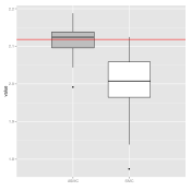
(a) parameter $\mu_{1}$

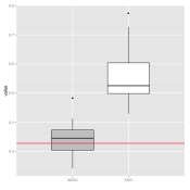
(b) parameter $\sigma_{1}$

Posterior mean of the parameters from both vanilla SMC (adaptive only in the exploration of the sequence). The white boxplot corresponds to the uniform kernel and the gray boxplot is given by the exponential kernel. We obtain the red line by sampling with ten times more particles. The two algorithm are run at constant computational time.

 

There is already a substantial computational gain in using the exponential kernel rather than the uniform. In the case of ABC this amounts to weighing the particles rather than just throwing away the particles that do not make a threshold. Intuitively at least, replacing the hard threshold by a soft one, should reduce the variance. Furthermore it seems from the experiments that exponentially weighted (EW) version could explore more quickly the sequence of posteriors. This will serve as a general justification for looking at the EW version from now on.

On the same experience we show the effect of increasing adaptively the number of samples $M$. We compare two SMC samplers with exponential weights, one with fixed $M=1$ and one that increases gradually $M$ according to the rule that was defined in Section 5.5.

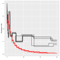
Figure 2: Acceptance ratio (multiple samples)

On the correctly specified data-set we show the evolution of the acceptance ration with the increase of the inverse temperature. The solid black line is given by the SMC-ABC with exponential kernel under with an adaptive choice of of parameter $M$ indexing the number of samples per particles. The red solid line is the corresponding value for the vanilla EW SMC-ABC. Similar behavior was observed for the case of the uniform kernel in Del Moral et al. (2012). The targeted acceptance ratio is 10%.

 

It is already known that for fixed $M$ the value of the acceptance ratio will decrease. In Figure 2 we see that the effect of using Gibbs sampling is to maintain the acceptance ratio at a given level. We also tested the importance sampling algorithm, the effect of changing the weights on this examples led to very high variance to the point that the weight degenerated to $0$ ($ESS=1$). Several additional point should be considered when using this algorithm. In particular the increase of $M$ has also an effect on the memory of the system as described at the beginning of Section 5. Different approach can be considered to treat this problem, in a technical note Chopin et al. (2015) propose to store seeds used for the pseudo-random number generator and to sample each trajectory each time it is needed. We do not delve further on those problems as they go beyond the aim of this paper. In the rest of the experiements we will use exponential weights and the adaptive selection of the number of particles in $M$ presented in sub-Section .

6.2 Experiment 2

We produce the same experiment as in the previous section, only this time the model is mis-specified. We consider for a true model a mixture of Gaussian with $3$ components. In the ABC pseudo-posterior we use for $\left\{\pi_{\theta},\theta\in\Theta\right\}$ the model described in the previous experiment. We show the median and the maximum mean square error of the statistics that are used in the pseudo posterior. The MSE does not totally cancel even for the ABC that we develop as there still exists a small bias. However we get a relatively small value. To obtain the necessary bounds (replicating the example of Section 4) we truncate the observation to the set $\left[-5,5\right]$ (this is equivalent to a change in the statistics). We can therefore also compare the performance of the algorithm with adaptive inverse temperature $\lambda$ (i.e. $\lambda$ is selected using by using the adaptive algorithm of Section 3.3).

Figure 3: Median and maximum MSE

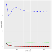
(a) Median MSE

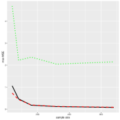
(b) Maximum MSE

We show the MSE corresponding to the algorithms described in the previous section. The blue dotted-dash line is the original SMC-ABC algorithm. Our adaptive SMC algorithm with $\lambda=90$ is given by the red dashed line. The green dotted line is the MSE obtained by using “true” samples from the false model. The solid black line is the MSE of our adptive SMC with adaptive chosen inverse temperature (algorithm of Section 3.3). All the computations are done at constant computational cost.

 

In Figure 3 we show as a function of the sample size the decrease in MSE. The algorithms are also compared to the loss that we would obtain from using the standard Bayesian posterior for the wrong model (blue line). We see that our exponential weight and adaptive exponential weight ABC (respectively solid black and dashed red lines) perform well in this framework.

We also give as an illustration the kind of empirical bounds one can get using Section 3.2. We show in Figure 4 a bound on the Euclidean distance between the moments of the statistics considered. The $y$-axis is given in logarithmic scale. We see that for certain value of the inverse temperature the bound on the generalized error is actually quite low. Recall however that we can not use directly the bound for choosing $\lambda$ as the bound is true in probability for individual values of the parameter. One could however use a union bound or the adaptive ABC described in Section 3.3. This is in fact very similar in nature.

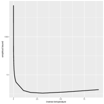
Figure 4: Empirical bound

As an illustration we show an empirical bound obtained for our algorithm under the misspecified setting. The bound is true up to 95% probability. The bound however as explained in Section 3 is not true jointly (i.e. for the whole value of $\lambda$ simultaneously). Here we can just observe the order of magnitude, implying that the algorithm has significantly learned from the data.

 

More details on the experiments can be found in appendix A.

6.3 Experiment 3

In this next experiment we use the same model, still under misspecification only we propose this time to use as summary statistics the sequence of indicator functions $\left(\textbf{1}_{x<t_{i}}\right)_{i=1}^{n}$ for a partition $\left(t_{i}\right)_{i}$ of the interval $[-5,5]$. The distance is taken to be the max-norm. Figure 5 illustrates the effect of combining the indicators functions as statistics and the distance based on the max-norm. The left panel shows that the max error of the ABC algorithm is smaller, this however leads to a uni-modal model (green curve on the right panel). On the other hand the MCMC sampler estimates a model with two distinct modes. This illustrates the importance of the choice of the different components (distance and summary statistics) as they have a direct impact on the final quantity one wants to control.

Figure 5: Indicators as a statistic

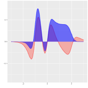
(a) Error on the statistics

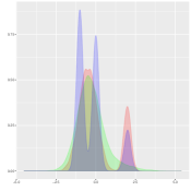
(b) Density, and predicted density

We show some results for the sequence of statistics $\left(\textbf{1}_{x<t_{i}}\right)_{i=1}^{n}$. On the left figure we show the difference between the statistics obtained from our sampler and the true statistics (averaged over the true model). In red we show the error obtained from the ABC sampler and in blue the one obtained from an MCMC sampler. On the right panel the estimated density of the observation (blue) and the predicted data according to the MCMC sampler (red ) and the ABC approximation (green).

 

7 Proofs and supporting results

7.1 Preliminary results

We start be recalling the following well known formulae (e.g. Catoni (2007) Chapter 1)

For any $\varrho\ll\pi$ and $h\in L^{1}(\varrho)$,

$$\mathcal{K}(\varrho,\pi_{e^{h}})=\lambda\int h{\rm d}\varrho+\mathcal{K}(\varrho,\pi)+\log\int\exp(-h){\rm d}\pi.$$

where $\pi_{e^{h}}:=\frac{e^{h}d\pi}{\pi\left[e^{h}\right]}$. This implies two well known facts

$$\pi_{e^{h}} =\arg\min_{\varrho\in\mathcal{M}_{+}^{1}(\Theta)}\left\{\int h{\rm d}\varrho+\mathcal{K}(\varrho,\pi)\right\},$$ (4)

$$-\log\int\exp(-h){\rm d}\pi =\min_{\varrho\in\mathcal{M}_{+}^{1}(\Theta)}\left\{\int h{\rm d}\varrho+\mathcal{K}(\varrho,\pi)\right\}.$$ (5)

We will use those two equations repeatedly in what follows.

Notation specific to the section

In this section we will use the following shorthand notation for any probability measure $\nu_{1}$,$\nu_{2}$,

$$w_{d}(\nu_{1},\nu_{2})=\int d(S(x),S(y))\nu_{1}(dx)\nu_{2}(dy).$$

7.2 Proof of Proposition 1

The proofs of this section follow closely the techniques used in Catoni (2007).

Lemma 6.

Under Assumption A(A1) for any $\varrho\in\mathcal{M}_{+}^{1}$, $\lambda\in\mathcal{I}$, $n\geq 1$ and $\epsilon>0$ jointly with probability at least $1-\epsilon$,

$$\omega_{d}(\varrho,\mathbb{P})\leq \omega_{d}\left(\varrho,\delta_{Y^{n}}\right)+\frac{1}{\lambda}\mathcal{K}(\varrho,\pi_{\theta}\pi)+\frac{f(n,\lambda)}{\lambda}+\frac{1}{\lambda}\log\frac{2}{\epsilon}$$ (6)

$$\omega_{d}\left(\varrho,\delta_{Y^{n}}\right) \leq\omega_{d}(\varrho,\mathbb{P})+\frac{1}{\lambda}\mathcal{K}(\varrho,\pi_{\theta}\pi)+\frac{f(n,\lambda)}{\lambda}+\frac{1}{\lambda}\log\frac{2}{\epsilon}.$$

Proof.

We start by making successive use of the equality in (4) on the first line, Markov’s inequality on the second and Assumption A(A1) on the third. For any $\eta>0$

$$\mathbb{P}\left(\sup_{\varrho\in\mathcal{M}_{1}^{+}(\Theta\times\mathcal{X}^{n})}\left\{\lambda\varrho(D_{n}^{S}-\mathbb{P}D_{n}^{S})-\mathcal{K}(\varrho,\pi_{\theta}\pi)+\eta\right\}\geq 0\right) =\mathbb{P}\left(\log m_{X}\left[e^{\lambda(D_{n}^{S}-\mathbb{P}D_{n}^{S})+\eta}\right]\geq 0\right)$$

$$\leq m_{X}\otimes\mathbb{P}\left[e^{\lambda(D_{n}^{S}-\mathbb{P}D_{n}^{S})+\eta}\right]$$

$$\leq e^{f(n,\lambda)+\eta}.$$

The inequality is true for any $\eta$ in particular choose $\eta=-\log\frac{1}{\epsilon}-f(n,\lambda)$,

$$\mathbb{P}\left(\sup_{\varrho\in\mathcal{M}_{1}^{+}(\Theta\times\mathcal{X}^{n})}\left\{\lambda\varrho(D_{n}^{S}-\mathbb{P}D_{n}^{S})-\mathcal{K}(\varrho,\pi_{\theta}\pi)\right\}-\log\frac{1}{\epsilon}-f(n,\lambda)\geq 0\right)\leq\epsilon.$$

Therefore for any $\varrho\in\mathcal{M}_{+}^{1}(\Theta\times\mathcal{X}^{n})$ with probability at least $1-\epsilon$ ,

$$\lambda\varrho(D_{n}^{S}-\mathbb{P}D_{n}^{S}) \leq\mathcal{K}(\varrho,\pi_{\theta}\pi)+f(n,\lambda)+\log\frac{1}{\epsilon}.$$ (7)

We note that owing to the symmetry of Assumption A(A1) we can apply the same reasoning to $-D_{n}^{S}$. Hence we get with probability at least $1-\epsilon$,

$$\lambda\varrho(\mathbb{P}D_{n}^{S}-D_{n}^{S}) \leq\mathcal{K}(\varrho,\pi_{\theta}\pi)+f(n,\lambda)+\log\frac{1}{\epsilon}.$$ (8)

We conclude the proof by applying a union bound to both equations, rearranging the terms and using the definition of $w_{d}$. ∎

The proof of the empirical bound (Proposition 1) can be obtain from equation (8). Using Assumption A(A2) and Jensen’s inequality with probability at least $1-\epsilon$,

$$d(\rho(S),\mathbb{P}(S))\leq\varrho(\mathbb{P}D_{n}^{S})\leq\rho\left(D_{n}^{S}\right)+\frac{1}{\lambda}\left(\mathcal{K}(\varrho,\pi_{\theta}\pi)+f(n,\lambda)+\log\frac{1}{\epsilon}\right).$$

This proves the first part of proposition 1, the second part is application of equation 5, by taking the infimum of the upper bound in $\rho\in\mathcal{M}_{+}^{1}$ we obtain the desired result.

7.3 Proof of Lemma 1

We start from the following lemma, a simple extension of Lemma 6,

Lemma 7.

Under Assumption A(A1), for any $\lambda\in\mathcal{I}$, $n\geq 1$and $\epsilon>0$ we have with probability at least $1-\epsilon$,

$$\omega_{d}(\varrho_{\lambda},\mathbb{P})\leq\inf_{\varrho\in\mathcal{M}_{+}^{1}(\Theta\times\mathcal{X}^{n})}\left\{\omega_{d}(\varrho,\mathbb{P})+\frac{2}{\lambda}\mathcal{K}(\varrho,\pi_{\theta}\pi)\right\}+2\frac{f(\lambda,n)}{\lambda}+\frac{2}{\lambda}\log\frac{2}{\epsilon}.$$

Proof.

By applying the inequalities of Lemma 6 to the case where $\varrho$ is the ABC measure and noticing that by equation 4 this measure is solution of the variational problem minimizing the empirical bound 6 we get jointly with probability at least $1-\epsilon$,

$$\omega_{d}(\varrho_{\lambda},\mathbb{P})\leq \inf_{\varrho\in\mathcal{M}_{+}^{1}(\Theta\times\mathcal{X}^{n})}\left\{\omega_{d}\left(\varrho,\delta_{Y^{n}}\right)+\frac{1}{\lambda}\mathcal{K}(\varrho,\pi_{\theta}\pi)\right\}+\frac{f(\lambda,n)}{\lambda}+\frac{1}{\lambda}\log\frac{2}{\epsilon}$$

$$\omega_{d}\left(\varrho_{\lambda},\delta_{Y^{n}}\right) \leq\omega_{d}(\varrho_{\lambda},\mathbb{P})+\frac{1}{\lambda}\mathcal{K}(\varrho_{\lambda},\pi_{\theta}\pi)+\frac{f(\lambda,n)}{\lambda}+\frac{1}{\lambda}\log\frac{2}{\epsilon}.$$

We get the desired result by combining both equations. ∎

The proof of Lemma 1 starts from noticing that under Assumption A(A2) we get from Lemma 7 by Jensen’s inequality, with probability at least $1-\epsilon$,

$$d(\varrho_{\lambda}(S),\mathbb{P}S)\leq\omega_{d}(\varrho_{\lambda},\mathbb{P})\leq\inf_{\varrho\in\mathcal{M}_{+}^{1}(\Theta\times\mathcal{X}^{n})}\left\{\omega_{d}(\varrho,\mathbb{P})+\frac{2}{\lambda}\mathcal{K}(\varrho,\pi_{\theta}\pi)\right\}+2\frac{f(\lambda,n)}{\lambda}+\frac{2}{\lambda}\log\frac{2}{\epsilon}.$$

Recall that the oracle parameter $\theta^{\star}$ is defined as the minimizer of $\theta\mapsto d(\pi_{\theta}(S),\mathbb{P}S)$ from definition 2. The infimum over all measures can be upper bounded by using the following parametric family,

$$\varrho_{\theta^{\star},\delta}(dX^{n},d\theta)=\frac{\pi_{\theta}(dX^{n})\pi(d\theta)\textbf{1}_{\|\theta-\theta^{\star}\|<\delta}}{\pi(\|\theta-\theta^{\star}\|<\delta)}.$$

we can therefore weaken the bound, with probability at least $1-\epsilon$,

$$d(\varrho_{\lambda}(S),\mathbb{P}S)\leq\inf_{\delta\in(0,\bar{\delta})}\left\{\omega_{d}(\varrho_{\theta^{\star},\delta},\mathbb{P})+\frac{2}{\lambda}\mathcal{K}(\varrho_{\theta^{\star},\delta},\pi_{\theta}\pi)\right\}+2\frac{f(\lambda,n)}{\lambda}+\frac{2}{\lambda}\log\frac{2}{\epsilon}.$$

Direct calculation yields that the KL divergence is expressed as,

$$\mathcal{K}(\varrho_{\theta^{\star},\delta},\pi_{\theta}\pi)=-\log\pi\left(\|\theta-\theta^{\star}\|<\delta\right).$$ (9)

It remains to deal with the term $\omega_{d}(\varrho_{\theta^{\star},\delta},\mathbb{P})$, we have from the triangle inequality,

$$d(S(X^{n}),S(Y^{n}))\leq d(S(X^{n}),\pi_{\theta}S)+d(\pi_{\theta}S,\pi_{\theta^{\star}}S)+d(\pi_{\theta^{\star}}S,\mathbb{P}S)+d(\mathbb{P}S,S(Y^{n})).$$

We use this inequality in the definition of $w_{d}$,

$$\omega_{d}(\varrho_{\theta^{\star},\delta},\mathbb{P}) =\int d(S(X^{n}),S(Y^{n}))\mathbb{P}(dY^{n})\frac{\pi_{\theta}(dX^{n})\pi(d\theta)\textbf{1}_{\|\theta-\theta^{\star}\|<\delta}}{\pi(\|\theta-\theta^{\star}\|<\delta)}$$

$$\leq\sup_{\theta:\|\theta-\theta^{\star}\|<\delta}\pi_{\theta}d(S,\pi_{\theta}S)+\int d(\pi_{\theta}S,\pi_{\theta^{\star}}S)\varrho_{\theta,\delta}(\rm{d}\theta)+d(\pi_{\theta^{\star}}S,\mathbb{P}S)+\mathbb{P}d(\mathbb{P}S,S))$$

Putting everything together yields the correct result.

7.4 Proof of Theorem 1

We start by using Assumption A(A4) and the triangle inequality

$$\varrho_{\lambda}\left\{\left\|\theta-\theta^{\star}\right\|\right\}\leq K\varrho_{\lambda}\left\{d\left(\pi_{\theta}S,\pi_{\theta^{\star}}S\right)\right\}\leq K\varrho_{\lambda}\left\{d\left(\pi_{\theta}S,S\right)\right\}+K\varrho_{\lambda}\left\{d\left(S,\mathbb{P}S\right)\right\}+Kd\left(\pi_{\theta^{\star}}S,\mathbb{P}S\right).$$

The second term on the right hand side is bounded above by Lemma 1, the last term is the oracle risk. We concentrate on the bound for $\varrho_{\lambda}\left\{d\left(\pi_{\theta}S,S\right)\right\}$.

We start by recalling the following well known fact, fix a probability measure $\pi$ then

$$\forall\varrho\in\mathcal{M}_{+}^{1},\lambda\in\mathbb{R}_{+\star}\quad\varrho(h)\leq\frac{1}{\lambda}\log\pi\left(e^{\lambda h}\right)+\frac{1}{\lambda}\mathcal{K}(\varrho,\pi).$$

We apply this inequality to $\varrho_{\lambda}\left\{d\left(\pi_{\theta}S,S\right)\right\}$ yielding

$$\varrho_{\lambda}\left\{d\left(\pi_{\theta}S,S\right)\right\} \leq\frac{1}{\lambda}\log\pi\pi_{\theta}\left(e^{\lambda d\left(\pi_{\theta}S,S\right)}\right)+\frac{1}{\lambda}\mathcal{K}\left(\varrho_{\lambda},\pi\pi_{\theta}\right)$$

$$\leq\frac{1}{\lambda}\log\pi\pi_{\theta}\left(e^{\lambda d\left(\pi_{\theta}S,S\right)}\right)-\frac{1}{\lambda}\log\pi\left(e^{-\lambda D_{n}^{S}}\right)-\varrho_{\lambda}\left(D_{n}^{S}\right),$$

where the last line comes from an expansion of the KL term. By positivity of the distance and by multiplication by $e^{\lambda\pi_{\theta}d\left(\pi_{\theta}S,S\right)}$ we get

$$\varrho_{\lambda}\left\{d\left(\pi_{\theta}S,S\right)\right\}\leq\frac{1}{\lambda}\log\pi\left\{\pi_{\theta}\left(e^{\lambda\left\{d\left(\pi_{\theta}S,S\right)-\pi_{\theta}d\left(\pi_{\theta}S,S\right)\right\}}\right)e^{\lambda\pi_{\theta}d\left(\pi_{\theta}S,S\right)}\right\}-\frac{1}{\lambda}\log\pi\left(e^{\lambda D_{n}^{S}}\right).$$

Under Assumption A(A5) we can bound the first part

$$\varrho_{\lambda}\left\{d\left(\pi_{\theta}S,S\right)\right\} \leq\frac{\tilde{f}(n,\lambda)}{\lambda}+\frac{1}{\lambda}\log\pi\left\{e^{\lambda\pi_{\theta}d\left(\pi_{\theta}S,S\right)}\right\}-\frac{1}{\lambda}\log\pi\left(e^{\lambda D_{n}^{S}}\right)$$

$$\leq\frac{\tilde{f}(n,\lambda)}{\lambda}+\sup_{\theta\in\Theta}\pi_{\theta}d\left(\pi_{\theta}S,S\right)+\inf_{\varrho\in\mathcal{M}_{1}^{+}}\left\{\varrho(D_{n}^{S})+\frac{1}{\lambda}\mathcal{K}(\varrho,\pi)\right\}.$$

It remains to treat the last part, notice that we can make use of equation (7) with probability a least $1-\epsilon$ we have

$$\varrho_{\lambda}\left\{d\left(\pi_{\theta}S,S\right)\right\}\leq\frac{\tilde{f}(n,\lambda)}{\lambda}+\sup_{\theta\in\Theta}\pi_{\theta}d\left(\pi_{\theta}S,S\right)+\inf_{\varrho\in\mathcal{M}_{1}^{+}}\left\{\varrho(\mathbb{P}D_{n}^{S})+\frac{2}{\lambda}\mathcal{K}(\varrho,\pi_{\theta}\pi)\right\}+\frac{1}{\lambda}\log\frac{1}{\epsilon}.$$

We can now use the developments of Lemma 1, putting $\varrho_{\theta^{\star},\delta}(dX^{n},d\theta)=\frac{\pi_{\theta}(dX^{n})\pi(d\theta)\textbf{1}_{\|\theta-\theta^{\star}\|<\delta}}{\pi(\|\theta-\theta^{\star}\|<\delta)}$

$$\inf_{\varrho\in\mathcal{M}_{1}^{+}}\left\{\varrho(\mathbb{P}D_{n}^{S})+\frac{2}{\lambda}\mathcal{K}(\varrho,\pi)\right\} \leq\inf_{\delta\in(0,\bar{\delta})}\left\{\omega_{d}(\varrho_{\theta^{\star},\delta},\mathbb{P})+\frac{2}{\lambda}\mathcal{K}(\varrho_{\theta^{\star},\delta},\pi_{\theta}\pi)\right\}$$

$$\leq\sup_{\theta:\|\theta-\theta^{\star}\|<\delta}\pi_{\theta}d(S,\mathbb{\pi_{\theta}}S)+\delta L+d(\pi_{\theta^{\star}}S,\mathbb{P}S)+\mathbb{P}d(\mathbb{P}S,S)-\log\pi\left(\|\theta-\theta^{\star}\|<\delta\right),$$

where we have used equation (9) and equation (LABEL:eq:triangle-ineq). We get the desired result by putting everything together and using a union bound.

7.5 Proof of Lemma 2

Let $\mathcal{I}\subset\mathbb{R}_{+}$be the possible range of the inverse temperature parameter. Define a prior measure $\nu$ on $(\mathcal{I},\mathcal{B}(\mathcal{I}))$. We follow the lines of the proof of Lemma 1 only the variational procedure is now taken on measures on $(\Theta\times\mathcal{X}^{n}\times\mathcal{I})$.

Lemma 8.

Under Assumption A(A1) for any $\mu\in\mathcal{M}_{+}^{1}(\Theta\times\mathcal{X}^{n}\times\mathcal{I})$, $n\geq 1$ and $\epsilon>0$ jointly with probability at least $1-\epsilon$,

$$\left.\begin{array}[]{c}\mu\left\{\lambda(\mathbb{P}D_{n}^{S}-D_{n}^{S})\right\}\\ \mu\left\{\lambda(D_{n}^{S}-\mathbb{P}D_{n}^{S})\right\}\end{array}\right\} \leq\mu\left[f(n,\lambda)\right]+\mathcal{K}\left(\mu,\left[\pi_{\theta}\pi\right]\otimes\nu\right)+\log\frac{2}{\epsilon}.$$

Proof.

Recall the starting point of the proof of Lemma 8, and use as before equations 4, 5, Markov’s inequality and Assumption A(A1),

$$\mathbb{P}\left(\sup_{\mu\in\mathcal{M}_{1}^{+}(\Theta\times\mathcal{X}^{n}\times\mathcal{I})}\left\{\mu\left\{\lambda(D_{n}^{S}-\mathbb{P}D_{n}^{S})+\eta(\lambda)\right\}-\mathcal{K}\left(\mu,\left[\pi_{\theta}\pi\right]\otimes\nu\right)\right\}\geq 0\right) =\mathbb{P}\left(\log\nu\otimes m_{X}\left[e^{\lambda(D_{n}^{S}-\mathbb{P}D_{n}^{S})+\eta}\right]\geq 0\right)$$

$$\leq\nu\otimes m_{X}\mathbb{\otimes P}\left[e^{\lambda(D_{n}^{S}-\mathbb{P}D_{n}^{S})+\eta(\lambda)}\right]$$

$$\leq\nu\left[e^{f(n,\lambda)+\eta(\lambda)}\right]$$

by choosing $\eta(\lambda)=-\log\frac{1}{\epsilon}-f(n,\lambda)$ we get,

$$\mathbb{P}\left(\sup_{\mu\in\mathcal{M}_{1}^{+}(\Theta\times\mathcal{X}^{n}\times\mathcal{I})}\left\{\mu\left\{\lambda(D_{n}^{S}-\mathbb{P}D_{n}^{S})-f(n,\lambda)\right\}-\mathcal{K}\left(\mu,\left[\pi_{\theta}\pi\right]\otimes\nu\right)\right\}\geq\log\frac{1}{\epsilon}\right)\leq\epsilon.$$

Hence for any $\mu\in\mathcal{M}_{1}^{+}(\Theta\times\mathcal{X}^{n}\times\mathcal{I})$ with probability at least $1-\epsilon$,

$$\mu\left\{\lambda(D_{n}^{S}-\mathbb{P}D_{n}^{S})\right\}\leq\mu\left[f(n,\lambda)\right]+\mathcal{K}\left(\mu,\left[\pi_{\theta}\pi\right]\otimes\nu\right)+\log\frac{1}{\epsilon}.$$

By symmetry we get for any $\mu\in\mathcal{M}_{1}^{+}(\Theta\times\mathcal{X}^{n}\times\mathcal{I})$ with probability at least $1-\epsilon$,

$$\mu\left\{\lambda(\mathbb{P}D_{n}^{S}-D_{n}^{S})\right\}\leq\mu\left[f(n,\lambda)\right]+\mathcal{K}\left(\mu,\left[\pi_{\theta}\pi\right]\otimes\nu\right)+\log\frac{1}{\epsilon}.$$

We conclude using a union bound. ∎

In what follows we will restrict ourselves on a specific kind of factorizable measures that allow us to further perform calculations. We let $\mu=\rho\otimes\xi\in\mathcal{M}_{1}^{+}(\Theta\times\mathcal{X}^{n})\times\mathcal{M}_{1}^{+}(\mathcal{I})\subset\mathcal{M}_{1}^{+}(\Theta\times\mathcal{X}^{n}\times\mathcal{I})$, and deduce from lemma 8 the following result,

Lemma 9.

Under Assumption A(A1) for any $\rho\in\mathcal{M}_{1}^{+}(\Theta\times\mathcal{X}^{n})$, $\xi\in\mathcal{M}_{1}^{+}(\mathcal{I})$, $n\geq 1$ and $\epsilon>0$ jointly with probability at least $1-\epsilon$,

$$\rho_{\hat{\xi}(\lambda)}\left[\mathbb{P}D_{n}^{S}\right]\leq\inf_{\xi\in\mathcal{F}}\left\{\inf_{\rho\in\mathcal{M}_{1}^{+}(\Theta\times\mathcal{X}^{n})}\left\{\rho(\mathbb{P}D_{n}^{S})+\frac{2}{\xi(\lambda)}\mathcal{K}\left(\rho,\pi_{\theta}\pi\right)\right\}+\frac{2}{\xi(\lambda)}\left(\xi\left[f(n,\lambda)\right]+\mathcal{K}\left(\xi,\nu\right)+\log\frac{2}{\epsilon}\right)\right\}.$$

Proof.

We get by directly restraining the results of lemma 8 to the factorizable measure jointly with probability at least $1-\epsilon$,

$$\left.\begin{array}[]{c}\xi\left(\lambda\right)\rho(\mathbb{P}D_{n}^{S}-D_{n}^{S})\\ \xi\left(\lambda\right)\rho(D_{n}^{S}-\mathbb{P}D_{n}^{S})\end{array}\right\}\leq\xi\left[f(n,\lambda)\right]+\mathcal{K}\left(\rho,\pi_{\theta}\pi\right)+\mathcal{K}\left(\xi,\nu\right)+\log\frac{2}{\epsilon}.$$

We rewrite the first part of the equation for any $\rho\in\mathcal{M}_{1}^{+}(\Theta\times\mathcal{X}^{n})$, $\xi\in\mathcal{M}_{1}^{+}(\mathcal{I})$

$$\rho\left[\mathbb{P}D_{n}^{S}\right]\leq\rho(D_{n}^{S})+\frac{1}{\xi(\lambda)}\left(\xi\left[f(n,\lambda)\right]+\mathcal{K}\left(\rho,\pi_{\theta}\pi\right)+\mathcal{K}\left(\xi,\nu\right)+\log\frac{2}{\epsilon}\right).$$

One can take the best bound amongst possible measures,

$$\rho_{\tilde{\xi}(\lambda)}\left[\mathbb{P}D_{n}^{S}\right]\leq\inf_{\xi\in\mathcal{M}_{1}^{+}(\mathcal{I})}\left\{\inf_{\rho\in\mathcal{M}_{1}^{+}(\Theta\times\mathcal{X}^{n})}\left\{\rho(D_{n}^{S})+\frac{1}{\xi(\lambda)}\mathcal{K}\left(\rho,\pi_{\theta}\pi\right)\right\}+\frac{1}{\xi(\lambda)}\left(\xi\left[f(n,\lambda)\right]+\mathcal{K}\left(\xi,\nu\right)+\log\frac{2}{\epsilon}\right)\right\}.$$

Note that the two infimum are computed sequentially, starting with $\rho$, leading to a problem that can be computed for fixed $\xi$. Then the infimum in $\xi$.

The infimum over $\rho$ is achieved in the exponential weight measure with inverse temperature $\xi(\lambda)$ at $-\log Z_{\xi(\lambda)}$ by equations 4 and 5. The measure $\tilde{\xi}$ is the minimum achieved by $-\log Z_{\xi(\lambda)}+\frac{1}{\xi(\lambda)}\left(\xi\left[f(n,\lambda)\right]+\mathcal{K}\left(\xi,\nu\right)+\log\frac{2}{\epsilon}\right)$. By restricting the minimization to a specific class of probabilities $\mathcal{F}$ we therefore get the algorithm described in definition 3, we plug-in the second part of lemma 8 we get the result. ∎

As for the proof of lemma 1 we use Assumption A(A2) and Jensen’s inequality to get with probability at least $1-\epsilon$,

$$d(\rho_{\hat{\xi}(\lambda)}S,\mathbb{P}S)\leq\rho_{\hat{\xi}(\lambda)}\left[\mathbb{P}D_{n}^{S}\right]\leq\inf_{\xi\in\mathcal{F}}\left\{\inf_{\rho\in\mathcal{M}_{1}^{+}(\Theta\times\mathcal{X}^{n})}\left\{\rho(\mathbb{P}D_{n}^{S})+\frac{2}{\xi(\lambda)}\mathcal{K}\left(\rho,\pi_{\theta}\pi\right)\right\}+\frac{2}{\xi(\lambda)}\left(\xi\left[f(n,\lambda)\right]+\mathcal{K}\left(\xi,\nu\right)+\log\frac{2}{\epsilon}\right)\right\}.$$

Again we put

$$\varrho_{\theta^{\star},\delta}(dX^{n},d\theta)=\frac{\pi_{\theta}(dX^{n})\pi(d\theta)\textbf{1}_{\|\theta-\theta^{\star}\|<\delta}}{\pi(\|\theta-\theta^{\star}\|<\delta)}.$$

The rest of the proof goes along the line of the end of the proof of 1.

7.6 Proof of Section 4

7.6.1 Proof of Lemma 3

To prove the result we will start be defining a vector of observations with the $i$-th component replaced by $Y^{\prime},$ i.e. $Y^{n,\prime}=(Y_{1},\cdots,Y_{i-1},Y^{\prime},Y_{i},\cdots,Y_{n}).$ For this new sample we have by the triangle inequality

$$\left|d\left(S\left(Y^{n}\right),S\left(X^{n}\right)\right)-d\left(S\left(Y^{n,\prime}\right),S\left(X^{n}\right)\right)\right|\leq d\left(S\left(Y^{n,\prime}\right),S\left(Y^{n}\right)\right).$$

By the definition of $Y^{n,\prime}$ and $d$ the term on the right hand-side is $d\left(S\left(Y^{n,\prime}\right),S\left(Y^{n}\right)\right)=\frac{1}{n}\left\|H(Y_{i})-H(Y^{\prime})\right\|_{p}\leq\frac{2m^{\frac{1}{p}}K}{n}$. By the bounded difference inequality theorem 6.2 Boucheron et al. (2013) we get the desired result

7.6.2 Proof of Theorem 2

We can apply the lemma 1 to the framework of this section then with probability at least $1-\epsilon$,

$$d(\varrho_{\lambda}^{ABC}(S),\mathbb{P}(H))\leq\inf_{\theta\in\Theta}d(\pi_{\theta}(H),\mathbb{P}(H))+\sup_{\theta:\|\theta-\theta^{\star}\|\leq\delta}\pi_{\theta}\left\{d(S,\pi_{\theta}S)\right\}+\delta L+\mathbb{P}\left\{d(S,\mathbb{P}S)\right\}\\ +\frac{2\lambda K^{2}m^{\frac{2}{p}}}{n}-\frac{2}{\lambda}\log\pi\left(\left\{\|\theta-\theta^{\star}\|<\delta\right\}\right)+\frac{2}{\lambda}\log\frac{2}{\epsilon}.$$

We need to control $\mathbb{P}\left\{d(S,\mathbb{P}S)\right\}$ and $\pi_{\theta^{\star}}\left\{d(S,\pi_{\theta^{\star}}S)\right\}$, we use Jensen for the first inequality, on the third line we use Nemirovki’s inequality (see Boucheron et al. (2013) p. 335),

$$\mathbb{P}\left\{d(S,\mathbb{P}S)\right\} =\mathbb{P}\left\{\left\|\frac{1}{n}\sum_{i=1}^{n}H(Y_{i})-\mathbb{P}H\right\|_{p}\right\}$$

$$\leq\sqrt{\frac{1}{n^{2}}\mathbb{P}\left\{\left\|\sum_{i=1}^{n}H(Y_{i})-\mathbb{P}H\right\|_{p}^{2}\right\}}$$

$$\leq\sqrt{\frac{K(p,m)}{n^{2}}\sum_{i=1}^{n}\mathbb{P}\left\{\left\|H(Y_{i})-\mathbb{P}H\right\|_{p}^{2}\right\}},$$

where $K(p,m)=\min\left(m,p-1,2e\log m\right).$ Using the i.i.d. hypothesis and the definition of $C$ we get,

$$\mathbb{P}\left\{d(S,\mathbb{P}S)\right\} \leq\sqrt{\frac{K(p,m)}{n}\mathbb{P}\left\{\left\|H(Y_{i})-\mathbb{P}H\right\|_{p}^{2}\right\}}$$

$$\leq\sqrt{\frac{K(p,m)m^{\frac{2}{p}}}{n}m^{2}\max_{j\leq m}\mathbb{P}\left\{\left(h_{j}-\mathbb{P}h_{j}\right)^{2}\right\}}$$

$$\leq\frac{Cm^{\frac{1}{p}+1}}{\sqrt{n}}$$

We get a similar bound for $\pi_{\theta}$, $\pi_{\theta}\left\{d(S,\pi_{\theta}S)\right\}\leq\frac{Cm^{\frac{1}{p}+1}}{\sqrt{n}}$.

7.6.3 Proof of Corollary 1

We start by lower bounding the small probability,

$$\log\pi\left(\left\{\|\theta-\theta^{\star}\|_{2}<\delta\right\}\right) =\log\pi\left(\left\{\theta:\sum_{i=1}^{d}(\theta_{i}-\theta_{i}^{\star})^{2}\leq\delta^{2}\right\}\right)$$

$$\geq d\min_{i}\log\pi\left(\left\{\theta:(\theta-\theta_{i}^{\star})^{2}\leq\frac{\delta^{2}}{d}\right\}\right)$$

$$\geq d\min_{i}\log\int_{\frac{\theta_{i}^{\star}}{\sqrt{\vartheta}}-\frac{\delta}{\sqrt{\vartheta d}}}^{\frac{\theta_{i}^{\star}}{\sqrt{\vartheta}}+\frac{\delta}{\sqrt{\vartheta d}}}\Phi_{1}(dx;0,1)$$

$$\geq d\min_{i}\log\left(\frac{\delta}{2\sqrt{\vartheta d}}\varphi\left(\frac{\theta_{i}^{\star}}{\sqrt{\vartheta}}+\frac{\delta}{\sqrt{\vartheta d}}\right)\right)$$

$$=d\log\left(\frac{\delta}{2\sqrt{2\pi\vartheta d}}\exp\left[-\frac{1}{2}\left(\frac{1}{\sqrt{\vartheta}}+\frac{\delta}{\sqrt{\vartheta d}}\right)^{2}\right]\right)$$

$$\geq d\log\left\{\frac{\delta}{2\sqrt{2\pi\vartheta d}}\exp\left(-\frac{1}{\vartheta}-\frac{\delta^{2}}{\vartheta d}\right)\right\}$$

The bound can therefore be written,

$$\|\varrho_{\lambda}^{ABC}(H)-\mathbb{P}(H)\|_{p}\leq\inf_{\theta\in\Theta}\|\pi_{\theta}(H)-\mathbb{P}(H)\|_{p}+\frac{Cm^{\frac{1}{p}+1}}{\sqrt{n}}+L\delta+\frac{2\lambda K^{2}m^{\frac{2}{p}}}{n}+\frac{2d}{\lambda}\left\{\log\frac{2\sqrt{2\pi\vartheta d}}{\delta}+\frac{1}{\vartheta}+\frac{\delta^{2}}{\vartheta d}\right\}+\frac{2}{\lambda}\log\frac{2}{\epsilon}.$$

We get the result by plugging$\lambda=\sqrt{\frac{dn}{K^{2}m^{\frac{2}{p}}}}$ and $\delta=\sqrt{\frac{\vartheta}{n}}$.

7.6.4 Proof of Corollary 2

We start by the result of Theorem 3,

$$\left\|\varrho_{\epsilon,\hat{\xi}}(H)-\mathbb{P}H\right\|_{p}\leq\inf_{\theta\in\Theta}\left\|\pi_{\theta}(S)-\mathbb{P}(S)\right\|_{p}+\frac{2Cm^{\frac{1}{p}}}{\sqrt{n}}e^{L\delta^{\alpha}}\\ +\inf_{\xi\in\mathcal{F}}\left[\frac{1}{\xi(\lambda)}\left\{2\xi\left[\lambda^{2}\right]\frac{K^{2}m^{\frac{2}{p}}}{n}-2\log\pi\left(\left\{\|\theta-\theta^{\star}\|<\delta\right\}\right)+2\mathcal{K}(\xi,\nu)+2\log\frac{2}{\epsilon}\right\}\right],$$

we need to compute the Kullback-Leibler term and the first and second order moments under an exponential distribution. We have,

$$\mathcal{K}(\xi,\nu) =\log\frac{\beta}{\alpha}+\frac{\alpha-\beta}{\beta},$$

$$\xi(\lambda) =\frac{1}{\beta},$$

$$\xi(\lambda^{2}) =\frac{2}{\beta^{2}}.$$

We plug those results in the above equation,

$$\left\|\varrho_{\epsilon,\hat{\xi}}(H)-\mathbb{P}H\right\|_{p}\leq\inf_{\theta\in\Theta}\left\|\pi_{\theta}(S)-\mathbb{P}(S)\right\|_{p}+2\frac{Cm^{\frac{1}{p}+1}}{\sqrt{n}}+L\delta\\ +\inf_{\beta\in\mathbb{R}_{+}}\left[\beta\left\{\frac{4}{\beta^{2}}\frac{K^{2}m^{\frac{2}{p}}}{n}-2\log\pi\left(\left\{\|\theta-\theta^{\star}\|<\delta\right\}\right)+2\log\frac{\beta}{\alpha}+2\frac{\alpha-\beta}{\beta}+2\log\frac{2}{\epsilon}\right\}\right].$$

Using the same bound as in corollary 1 for the small ball under the prior we get,

$$\left\|\varrho_{\epsilon,\hat{\xi}}(H)-\mathbb{P}H\right\|_{p}\leq\inf_{\theta\in\Theta}\left\|\pi_{\theta}(S)-\mathbb{P}(S)\right\|_{p}+2\frac{Cm^{\frac{1}{p}+1}}{\sqrt{n}}+L\delta\\ +\inf_{\beta\in\mathbb{R}_{+}}\left[\frac{4}{\beta}\frac{K^{2}m^{\frac{2}{p}}}{n}+2d\beta\left\{\log\frac{2\sqrt{2\pi\vartheta d}}{\delta}+\frac{1}{\vartheta}+\frac{\delta^{2}}{\vartheta d}\right\}+2\beta\log\frac{\beta}{\alpha}+2\left(\alpha-\beta\right)+2\beta\log\frac{2}{\epsilon}\right].$$

Using the fact that $\alpha<\beta$ otherwise the Kullback-Leibler does not exist, and putting $\beta=\sqrt{\frac{K^{2}m^{\frac{2}{p}}}{nd}}$, we get

$$\left\|\varrho_{\epsilon,\hat{\xi}}(H)-\mathbb{P}H\right\|_{p}\leq\inf_{\theta\in\Theta}\left\|\pi_{\theta}(S)-\mathbb{P}(S)\right\|_{p}+2\frac{Cm^{\frac{1}{p}+1}}{\sqrt{n}}+L\delta+4Km^{\frac{1}{p}}\sqrt{\frac{d}{n}}+2Km^{\frac{1}{p}}\sqrt{\frac{d}{n}}\left\{\log\frac{2\sqrt{2\pi\vartheta d}}{\delta}+\frac{1}{\vartheta}+\frac{\delta^{2}}{\vartheta d}\right\}\\ +\frac{Km^{\frac{1}{p}}}{\sqrt{nd}}\log\left(\frac{K^{2}m^{\frac{2}{p}}}{nd\alpha}\right)+2\frac{Km^{\frac{1}{p}}}{\sqrt{nd}}\log\frac{2}{\epsilon}.$$

Put $\delta=\sqrt{\frac{\vartheta}{n}}$ to get the result.

7.6.5 Proof of Lemma 4

As for the proof of lemma 3 define a sample $Y^{\prime,n}=\left(Y_{1},\cdots,Y^{\prime},\cdots Y_{n}\right)$ where the $i$-th sample has been replaced by $Y^{\prime}$ with the same distribution. By the triangular inequality,

$$\left|d(S(X^{n}),S(Y^{n}))-d(S(X^{n}),S(Y^{n,\prime}))\right|\leq d(S(Y^{n}),S(Y^{n,\prime})),$$

hence in this case $d(S(Y^{n}),S(Y^{n,\prime}))=\sqrt{\frac{1}{n^{2}}(Y_{i}-Y^{\prime})}\leq\sqrt{\frac{2K}{n^{2}}}.$ Hence by applying the bounded difference inequality Boucheron et al. (2013) we get the result.

7.6.6 Proof of Lemma 5

From Lemma 5.3. of van der Vaart et al. (2008) we get that the non-centered Gaussian small ball probability is characterized by its concentration function, i.e. for any $f^{\star}$ in the support,

$$-\log\pi\left[\left\|f-f^{\star}\right\|<\delta\right]\leq\inf_{h\in\mathbb{H}:\left\|h-f^{\star}\right\|\leq\frac{\delta}{2}}\frac{1}{2}\left\|h\right\|_{\mathbb{H}}^{2}-\log\pi\left[\left\|f\right\|<\frac{\delta}{2}\right],$$

where $\left(\mathbb{H},\left\|.\right\|_{\mathbb{H}}\right)$ is the reproducing kernel Hilbert space of the Gaussian variable $f$. van der Vaart et al. (2007) give a bound for the two quantities in the right hand-side, in the case where the Gaussian process has a spectral measure with exponentially decreasing tails and $f^{\star}\in\mathcal{H}^{\beta}\left(\left[0,1\right]\right)$. The condition on the spectral measure is satisfied in particular for the centered Gaussian process with Gaussian kernel. Suppose that the Gaussian process is re scaled with parameter $c\leq 1$ then by Theorem 2.4 van der Vaart et al. (2007) there exists $\delta_{0}>0$ and a constant $K$ such that for any $\delta\in(0,\delta_{0})$ the centered small ball probability satisfies,

$$-\log\pi\left[\left\|f\right\|<2\delta\right]\leq\frac{K}{c}\left(\log\frac{1}{c\delta^{2}}\right)^{2}.$$

Lemma 2.2 of the same paper gives a bound for the second part of the concentration function, under the assumption on $\pi$ and $f^{\star}$ there exist constants $D_{f^{\star}}$ and $C_{f^{\star}}$ depending only on $f^{\star}$ such that

$$\inf_{h\in\mathbb{H}:\left\|h-f^{\star}\right\|\leq C_{f^{\star}}c^{\beta}}\frac{1}{2}\left\|h\right\|_{\mathbb{H}}^{2}\leq D_{f^{\star}}\left(\frac{1}{c}\right).$$

Choosing $c$ such that $c^{\beta}\leq\delta$, we get the result by combining the two bounds.

7.6.7 Proof of Theorem 4

We start with lemma 1 applied to the framework of this section, with probability at least $1-\epsilon$,

$$d(\varrho_{\lambda}^{ABC}(S),\mathbb{P}(H))\leq\inf_{\theta\in\Theta}d(\pi_{\theta}(H),\mathbb{P}(H))+\sup_{\theta:\|\theta-\theta^{\star}\|}\pi_{\theta}\left\{d(S,\pi_{\theta}S)\right\}+L\delta+\mathbb{P}\left\{d(S,\mathbb{P}S)\right\}\\ +\frac{\lambda K}{n}-\frac{2}{\lambda}\log\pi\left(\left\{\|\theta-\theta^{\star}\|<\delta\right\}\right)+\frac{2}{\lambda}\log\frac{2}{\epsilon}.$$

We start as before to bound $\pi_{\theta}\left\{d(S,\pi_{\theta}S)\right\}$ and $\mathbb{P}\left\{d(S,\mathbb{P}S)\right\}$,

$$\pi_{\theta}\left\{d(S,\pi_{\theta}S)\right\} =\pi_{\theta}\left\{\sqrt{\frac{1}{n^{2}}\sum_{i=1}^{n}\left[X_{i}-\pi_{\theta}\left(X_{i}\right)\right]{}^{2}}\right\}$$

$$\leq\sqrt{\pi_{\theta}\left\{\frac{1}{n^{2}}\sum_{i=1}^{n}\left[X_{i}-\pi_{\theta}\left(X_{i}\right)\right]{}^{2}\right\}}$$

$$\leq\frac{1}{\sqrt{n}}\sup_{i}\sqrt{\mathbb{\mathbb{\pi_{\theta}}}\left\{\left(X_{i}-\pi_{\theta}(X_{i})\right)^{2}\right\}}.$$

We get a similar bound for $\mathbb{P}\left\{d(S,\mathbb{P}S)\right\}$, hence

$$d(\varrho_{\lambda}^{ABC}(S),\mathbb{P}(H))\leq\inf_{\theta\in\Theta}d(\pi_{\theta}(H),\mathbb{P}(H))+\frac{1}{\sqrt{n}}C+\frac{\lambda K}{n}\\ -\frac{2}{\lambda}\log\pi\left(\left\{\|\theta-\theta^{\star}\|<\delta\right\}\right)+\frac{2}{\lambda}\log\frac{2}{\epsilon}.$$

From lemma 5 we get an estimate of the prior concentration, we get that for $\delta_{n}\geq c_{n}^{\beta},$

$$d(\varrho_{\lambda}^{ABC}(S),\mathbb{P}(H))\leq\inf_{\theta\in\Theta}d(\pi_{\theta}(H),\mathbb{P}(H))+\frac{1}{\sqrt{n}}C+L\delta+\frac{\lambda K}{n}\\ +\frac{2}{\lambda}\left[D_{0}\left(\frac{1}{c_{n}}\right)+C_{0}\frac{1}{c_{n}}\left(\log\frac{1}{c_{n}\delta_{n}}\right)^{2}\right]+\frac{2}{\lambda}\log\frac{2}{\epsilon}.$$

Now we put $\delta_{n}\asymp\left(\frac{\log^{2}n}{n}\right)^{\frac{\beta}{2\beta+1}}$, $c_{n}\asymp\left(\frac{\log^{2}n}{n}\right)^{\frac{1}{2\beta+1}}$ and $\lambda_{n}\asymp n^{\frac{\beta+1}{2\beta+1}}\left(\log n\right)^{\frac{\beta}{2\beta+1}}$ to get the result for $n$ sufficiently large as to ensure $\delta_{n}<\bar{\delta}$.

8 Summary

We have explored convergence results for the ABC algorithm in the specific case of the exponential kernel. This kernel is introduced for technical reasons, in particular because it is the solution of a variational problem. The results in the paper suggest that ABC can be used in a mispecified scenario (i.e. $\mathbb{P}\notin\left\{\pi_{\theta},\theta\in\Theta\right\}$ in the notations of the paper), at the cost of choosing a larger window in the kernel. In particular it is instructive to note that we do not want this parameter to go to zero too fast even if it was possible computationally. We obtain oracle inequalities for the expected statistics under the ABC distribution. We show that they can be extended in some cases to oracle inequalities in the parameter space. The results rely mostly on the exponential concentration of the distance and some regularity of the model around the oracle parameter. One could remove the need for concentration inequalities on this problem by using the techniques introduced in Grünwald and Mehta (2016); Mendelson (2014); Alquier and Ridgway (2017); Bhattacharya et al. (2017), we leave this for a future study. A nice aspect of the result is that they are given for finite sample sizes and in deviation.

We also showed that we can obtain empirical bounds and adaptive oracle inequalities in the bandwidth. The proposed bounds can be used to gain intuition on the distance to choose and the size of the summary statistics for a given problem.

Finally we suggest some methodological improvement to the previously known SMC-ABC of Del Moral et al. (2012), allowing for further adaptation. We would like to stress at this point that, although we believe that SMC can perform well on this kind of problems, it is by no means the only approach to sample from the pseudo distribution.

Acknowledgments

I would like to warmly thank Pierre Alquier and Nicolas Chopin for the helpful discussions and comments.

Appendix A Implementation Details

We describe some building blocks of the algorithms of Section 5

Algorithm 5 Systematic resampling

Input:

Normalised weights $W_{t}^{j}:=w_{t}(\theta_{t-1}^{j})/\sum_{i=1}^{N}w_{t}(\theta_{t-1}^{i})$.

Output:

indices $A^{i}\in\{1,\ldots,N\}$, for $i=1,\ldots,N$.

a.

Sample $U\sim\mathcal{U}nif_{[0,1]}$.

b.

Compute cumulative weights as

c.

Set $s\leftarrow U$, $m\leftarrow 1$.

d.

For $n=1:N$

       While $C^{m}<s$ do $m\leftarrow m+1$.

       $A^{n}\leftarrow m$, and $s\leftarrow s+1$.

    End For

	In common	Tested
Figure 1	Algorithm are all versions of Del Moral et al. [2012]	One algorithm with exponential weights the other with uniform weigths
Figure 2	Algorithm are all versions of Del Moral et al. [2012] with exponential weights	On has adaptive choice of $M$ not the other
Figure 3	Algorithm are all versions of Del Moral et al. [2012] with exponential weights and adaptive choice $M$	One with fixed temperature, one with adaptive temperature and one is the algorithm of Del Moral et al. [2012] for a benchmark

References

- Alquier and Ridgway [2017] P. Alquier and J Ridgway. Concentration of tempered posterior and their variational approximations. arXiv:1706.09293, pages 1–24, 2017.
- Alquier et al. [2016] P. Alquier, J. R., and N. Chopin. On the properties of variational approximations of Gibbs posterior. Journal of Machine Learning Research, 17(239):1–41, 2016.
- Andrieu et al. [2010] C. Andrieu, A. Doucet, and R. Holenstein. Particle Markov Chain Monte Carlo. J. R. Statist. Soc. B, 72:269–342, 2010.
- Barber et al. [2015] S. Barber, J. Voss, and M. Webster. The rate of convergence for approximate Bayesian computation. Electronic Journal of Statistics, 9(1):80–105, 2015.
- Beaumont et al. [2002] M. A Beaumont, W. Zhang, and D. J Balding. Approximate Bayesian computation in population genetics. Genetics, 162(4):2025–2035, 2002.
- Bernton et al. [2017] E. Bernton, P. E Jacob, M. Gerber, and C. P Robert. Inference in generative models using the Wasserstein distance. arXiv preprint arXiv:1701.05146, 2017.
- Bhattacharya et al. [2017] A. Bhattacharya, D. Pati, and Y. Yang. Bayesian fractional posteriors. arxiv preprint, 2017.
- Boucheron et al. [2013] S. Boucheron, G. Lugosi, and P. Massart. Concentration inequalities: A nonasymptotic theory of independence. Oxford university Press, 2013.
- Cameron and Pettitt [2012] E. Cameron and AN Pettitt. Approximate Bayesian Computation for astronomical model analysis: a case study in galaxy demographics and morphological transformation at high redshift. Monthly Notices of the Royal Astronomical Society, 425(1):44–65, 2012.
- Catoni [2007] O. Catoni. PAC-Bayesian Supervised Classification, volume 56. IMS Lecture Notes & Monograph Series, 2007.
- Chopin et al. [2013] N. Chopin, O. Papaspiliopoulos, and P. E. Jacob. SMC2: an efficient algorithm for sequential analysis of state space models. J. R. Statist. Soc. B, 75(3):397–426, 2013.
- Chopin et al. [2015] N. Chopin, J. Ridgway, M. Gerber, and O. Papaspiliopoulos. Towards automatic calibration of the number of state particles within the SMC2 algorithm. technial report, 2015.
- Del Moral et al. [2006] P. Del Moral, A. Doucet, and A. Jasra. Sequential Monte Carlo samplers. J. R. Statist. Soc. B, 68(3):411–436, 2006. ISSN 1467-9868.
- Del Moral et al. [2012] P. Del Moral, A. Doucet, and A. Jasra. An adaptive sequential Monte Carlo method for approximate Bayesian computation. Statistics and Computing, 22(5):1009–1020, 2012. ISSN 1573-1375. 10.1007/s11222-011-9271-y. URL http://dx.doi.org/10.1007/s11222-011-9271-y.
- Fearnhead and Prangle [2012] P. Fearnhead and D. Prangle. Constructing Summary Statistics for Approximate Bayesian Computation: Semi-automatic ABC. J. R. Statist. Soc. B, 74:1–28, 2012.
- Frazier et al. [2016] D. T Frazier, G. M Martin, C. P Robert, and J. Rousseau. Asymptotic properties of approximate bayesian computation. arXiv preprint arXiv:1607.06903, 2016.
- Grelaud et al. [2009] A. Grelaud, C. P Robert, J. Marin, F. Rodolphe, and J. Taly. Abc likelihood-free methods for model choice in gibbs random fields. Bayesian Analysis, 4(2):317–335, 2009.
- Grünwald [2011] P. Grünwald. Safe learning: bridging the gap between bayes, mdl and statistical learning theory via empirical convexity. In Alt, 2011.
- Grünwald and Mehta [2016] P. Grünwald and N. Mehta. Fast rates with unbounded losses. arXiv preprint arXiv:1605.00252, 2016.
- Grünwald and van Ommen [2014] P. Grünwald and T. van Ommen. Inconsistency of bayesian inference for misspecified linear models, and a proposal for repairing it. arXiv preprint arXiv:1412.3730, 2014.
- Jasra et al. [2011] A. Jasra, D. A Stephens, A. Doucet, and T. Tsagaris. Inference for Lévy-Driven Stochastic Volatility Models via Adaptive Sequential Monte Carlo. Scandinavian Journal of Statistics, 38(1):1–22, 2011.
- Li and Fearnhead [2015] W. Li and P. Fearnhead. On the Asymptotic Efficiency of ABC Estimators. arXiv preprint arXiv:1506.03481, 2015.
- Mansinghka et al. [2013] Vikash Mansinghka, Tejas D Kulkarni, Yura N Perov, and Josh Tenenbaum. Approximate bayesian image interpretation using generative probabilistic graphics programs. In Advances in Neural Information Processing Systems, pages 1520–1528, 2013.
- Marin et al. [2012] J. Marin, P. Pudlo, C. P. Robert, and R. J. Ryder. Approximate bayesian computational methods. Statistics and Computing, 22(6):1167–1180, 2012. ISSN 1573-1375. 10.1007/s11222-011-9288-2. URL http://dx.doi.org/10.1007/s11222-011-9288-2.
- Marin et al. [2014] J. Marin, N. S Pillai, C. P Robert, and J. Rousseau. Relevant statistics for bayesian model choice. Journal of the Royal Statistical Society: Series B (Statistical Methodology), 76(5):833–859, 2014.
- Mendelson [2014] Shahar Mendelson. Learning without concentration. In COLT, pages 25–39, 2014.
- Olivier et al. [2010] Wintenberger Olivier et al. Deviation inequalities for sums of weakly dependent time series. Electronic Communications in Probability, 15:489–503, 2010.
- Press [2007] William H Press. Numerical recipes 3rd edition: The art of scientific computing. Cambridge university press, 2007.
- Rasmussen and Williams [2006] C. Rasmussen and C. Williams. Gaussian processes for Machine Learning. MIT press, 2006.
- Ridgway [2015] J Ridgway. Computation of Gaussian orthant probabilities in high dimension. Statistics and computing, pages 1–18, 2015.
- van der Vaart et al. [2007] Aad van der Vaart, Harry van Zanten, et al. Bayesian inference with rescaled Gaussian process priors. Electronic Journal of Statistics, 1:433–448, 2007.
- van der Vaart et al. [2008] Aad W van der Vaart, J Harry van Zanten, et al. Reproducing kernel Hilbert spaces of Gaussian priors. In Pushing the limits of contemporary statistics: contributions in honor of Jayanta K. Ghosh, pages 200–222. Institute of Mathematical Statistics, 2008.
- Zhang et al. [2006] Tong Zhang et al. From -entropy to kl-entropy: Analysis of minimum information complexity density estimation. The Annals of Statistics, 34(5):2180–2210, 2006.