Orthogonal and Idempotent Transformations for Learning Deep Neural Networks

Abstract

Identity transformations, used as skip-connections in residual networks, directly connect convolutional layers close to the input and those close to the output in deep neural networks, improving information flow and thus easing the training. In this paper, we introduce two alternative linear transforms, orthogonal transformation and idempotent transformation. According to the definition and property of orthogonal and idempotent matrices, the product of multiple orthogonal (same idempotent) matrices, used to form linear transformations, is equal to a single orthogonal (idempotent) matrix, resulting in that information flow is improved and the training is eased. One interesting point is that the success essentially stems from feature reuse and gradient reuse in forward and backward propagation for maintaining the information during flow and eliminating the gradient vanishing problem because of the express way through skip-connections. We empirically demonstrate the effectiveness of the proposed two transformations: similar performance in single-branch networks and even superior in multi-branch networks in comparison to identity transformations.

1 Introduction

Training convolution neural networks becomes more difficult with the depth increasing and even the training accuracy deceases for very deep networks. Identity mappings or transformations, which are adopted as skip-connections in deep residual networks [7], ease the training of very deep networks and make the accuracy improved.

Identity transformations lead to shorter connections between layers close to the input and those close to the output. It is shown that identity transformations improve information flow in both forward propagation and back-propagation because the product of identity matrices is still an identity matrix, in other words, multiple skip-connections is essentially like a single skip-connection no matter how many skip-connections there are.

In this paper, we introduce two linear transformations and use them as skip-connections for improving information flow. The first one is an orthogonal transformation. Multiplying several orthogonal matrices, used to form the orthogonal transformations, yields an orthogonal matrix. The benefit is that information attenuation and explosion is avoided because the absolute values of the eigenvalues of an orthogonal matrix are always $1$. The second one is an idempotent transformation, whose transformation matrix is an idempotent matrix which, when multiplied by itself, yields itself. A sequence of idempotent transformations with the same idempotent matrices is equivalent to a single idempotent transformation. We show that the success essentially comes from feature reuse and gradient reuse in forward and backward propagation for maintaining the information and eliminating the gradient vanishing problem because of the express way through skip-connections.

The empirical results show that single-branch deep neural networks with idempotent and orthogonal transformations as skip-connections achieve perform similarly to those with identity transformations and that the performances are superior when applied to multi-branch networks.

2 Related Works

In general, deeper convolutional neural networks leads to superior classification accuracy. An example is the improvement on the ImageNet classification from AlexNet [13] ($7$ layers) to VGGNet [21] ($19$ layers). However, going deeper increases the training difficulty. Techniques to ease the training include optimization techniques [18, 6, 4, 11, 5, 17, 19] and network architecture design. In the following, we discuss representative works on network architecture design.

GoogLeNet [23] is one of the first works, designing network architectures to deal with the difficulty of training deep networks. It is built by repeating Inception blocks each of which contains short and long branches, and thus there are both short and long paths between layers close to the input layer and those close to the output layer, i.e., information flow is improved.

Inspired by Long Short-Term Memory recurrent networks, highway networks [22] adopt identity transformations together with adaptive gating mechanism, allowing computation paths along which information can flow across many layers without attenuation. It indeed eases the training of very deep networks, e.g., $100$ layers. Residual networks [7] also adopt identity transformations as skip-connections, but without including gating units, making training networks of thousands of layers easier. In this paper, we introduce two alternative transformations, orthogonal and idempotent transformations, which also improve information flow. We do not find that they learn residuals as claimed in [7] and but find that features and gradients are reused through the express way composed of skip-connections.

FractalNets [14], deeply-fused nets [26], and DenseNets [9] present various multi-branch structures, leading to short and long paths between layers close to the input layer and those close to the output layer. Consequently, the effective depth [14] or the average depth [26] is reduced a lot though the nominal depth is great and accordingly information flow is improved.

Deep supervision [15] associates a companion local output and accordingly a loss function with each hidden layer, which results in shorter paths from hidden layers to the loss layers. Its success provides an evidence that effective depth is crucial. FitNets [20], a student-teacher paradigm, train a thinner and deeper student network such that the intermediate representations approach the intermediate representations of a wider and shallower (but still deep) teacher network that is relatively easy to be trained, which is in some sense a kind of deep supervision, also reducing the effective depth.

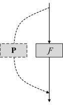
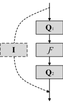
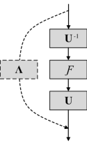
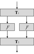
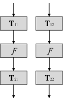
Figure 1: (a) A building block with a linear transformation $\mathbf{P}$; (b) An equivalent form for an orthogonal transformation; $\mathbf{Q}_{1}$ and $\mathbf{Q}_{2}$ correspond to pre-orthogonal transformation and post-orthogonal transformation. (c) An equivalent form for an idempotent transformation. (d) The regular connection with two branches converted from an orthogonal or idempotent transformation, where $\mathbf{T}_{1}$ and $\mathbf{T}_{2}$ are pre-linear transformation and post-linear transformation. (e) Two separate branches, where $\mathbf{T}_{11}$ ($\mathbf{T}_{12}$) and $\mathbf{T}_{21}$ ($\mathbf{T}_{22}$) are pre-linear transformation and post-linear transformation. The network in (d) cannot be converted to that in (e) for general pre- and post-transformations.

3 Orthogonal and Idempotent Transformations

A building block with a linear transformation used as the skip-connection is written as:

$$\mathbf{y} =\mathbf{P}\mathbf{x}+\mathcal{F}(\mathbf{x},\mathcal{W}).$$ (1)

Here, $\mathbf{x}$ and $\mathbf{y}$ are the input and output features. $\mathbf{P}\mathbf{x}$ is the skip-connection, and $\mathbf{P}$ is the transformation matrix. $\mathcal{F}$ is the regular connection, e.g., two convolutional layers with each followed by a ReLU activation function, and $\mathcal{W}$ is the parameters of the function $\mathcal{F}$. Following residual networks [7], we design the networks by starting with a convolutional layer, repeating such building blocks, and appending a global pooling layer and a fully-connected layer. Figure 1 illustrates such a block.

The recursive equations below show how the features are forward-propagated through building blocks and the gradients are backward-propagated.

Forward propagation. The transformation function, transferring the feature $\mathbf{x}_{m}$, the input of the $m$th building block to $\mathbf{x}_{n}$, the input of the $n$th building block, is given as follows,

$$\mathbf{x}_{n}=\mathbf{P}^{n-m}\mathbf{x}_{m}+\sum\nolimits_{i=m}^{n-1}\mathbf{P}^{n-i-1}\mathbf{x}^{\prime}_{i+1},$$ (2)

where $\mathbf{x}^{\prime}_{i+1}=\mathcal{F}(\mathbf{x}_{i},\mathcal{W}_{i})$, and $\mathbf{x}_{i}$ and $\mathcal{W}_{i}$ are the input and the parameters of the $i$th block.

Backward propagation. The gradient is backward-prorogated from $\mathbf{x}_{n}$ to $\mathbf{x}_{m}$ as below,

$$\frac{\partial\mathcal{L}}{\partial\mathbf{x}_{m}}=(\mathbf{P}^{n-m})^{\top}\frac{\partial\mathcal{L}}{\partial\mathbf{x}_{n}}+\sum\nolimits_{i=m}^{n-1}\frac{\partial\mathbf{x}^{\prime}_{i+1}}{\partial\mathbf{x}_{m}}(\mathbf{P}^{n-i-1})^{\top}\frac{\partial\mathcal{L}}{\partial\mathbf{x}_{n}},$$ (3)

where $\mathcal{L}$ is the loss function.

In the following, we show that the feature $\mathbf{x}_{m}$ is reused in any later feature $\mathbf{x}_{n}$ instead of only $\mathbf{x}_{m+1}$ and the gradient $\frac{\partial\mathcal{L}}{\partial\mathbf{x}_{n}}$ is reused in any early gradient $\frac{\partial\mathcal{L}}{\partial\mathbf{x}_{m}}$ such that the signal (information) is maintained and the vanishing problem is eliminated, for identity transformations, orthogonal transformations and idempotent transformations.

3.1 Identity transformations

Identity transformations, i.e., $\mathbf{P}=\mathbf{I}$, are adopted in residual networks [7]. The forward and backward processes are rewritten as below,

$$\mathbf{x}_{n} =\mathbf{x}_{m}+\sum\nolimits_{i=m}^{n-1}\mathbf{x}^{\prime}_{i+1},$$ (4)

$$\frac{\partial\mathcal{L}}{\partial\mathbf{x}_{m}} =\frac{\partial\mathcal{L}}{\partial\mathbf{x}_{n}}+\sum\nolimits_{i=m}^{n-1}\frac{\partial\mathbf{x}^{\prime}_{i+1}}{\partial\mathbf{x}_{m}}\frac{\partial\mathcal{L}}{\partial\mathbf{x}_{n}}.$$ (5)

It is obvious that there is a path along skip-connections, where (1) $\mathbf{x}_{m}$ directly flows to $\mathbf{x}_{n}$ though there are $(n-m)$ blocks; and (2) the gradient with respect to $\mathbf{x}_{n}$ is directly backward sent to the gradient with respect to $\mathbf{x}_{m}$ along the same path (both correspond to the first term of the right-hand side of the above two equations).

3.2 Orthogonal transformations

An orthogonal transformation is a linear transformation, where the transformation matrix is orthogonal. Mathematically, a matrix $\mathbf{Q}$ is orthogonal if $\mathbf{Q}^{\top}\mathbf{Q}=\mathbf{Q}\mathbf{Q}^{\top}=\mathbf{I}$. We have the following property:

Property 1.

The product of an arbitrary number of orthogonal matrices is orthogonal: $\prod_{k=1}^{K}\mathbf{Q}_{k}$ is orthogonal, if $\mathbf{Q}_{1},~{}\mathbf{Q}_{k},~{}\dots,~{}\mathbf{Q}_{K}$ are orthogonal.

Thus, the forward process (Equation 2) is rewritten as follows,

$$\mathbf{x}_{n}=\mathbf{Q}_{n-m}\mathbf{x}_{m}+\sum\nolimits_{i=m}^{n-1}\mathbf{Q}_{n-i-1}\mathbf{x}^{\prime}_{i+1},$$ (6)

where $\mathbf{Q}_{n-m}=\mathbf{Q}^{n-m}$ and $\mathbf{Q}_{n-i-1}=\mathbf{Q}^{n-i-1}$. We can see that $\mathbf{x}_{m}$ is sent to $\mathbf{x}_{n}$ via a single orthogonal transformation (corresponding to the first term of the right-hand side) One notable property is that any orthogonal transformation $\mathbf{Q}$ preserves the length of vectors: $\|\mathbf{Q}\mathbf{x}\|_{2}=\|\mathbf{x}\|_{2}$. This means that through the path formed by skip-connections, the norm of the vector is maintained.

The backward process (Equation 3) becomes

$$\frac{\partial\mathcal{L}}{\partial\mathbf{x}_{m}}=\mathbf{Q}_{n-m}^{\top}\frac{\partial\mathcal{L}}{\partial\mathbf{x}_{n}}+\sum\nolimits_{i=m}^{n-1}\frac{\partial\mathbf{x}^{\prime}_{i+1}}{\partial\mathbf{x}_{m}}\mathbf{Q}_{n-i-1}^{\top}\frac{\partial\mathcal{L}}{\partial\mathbf{x}_{n}}.$$ (7)

Again, there is a path, formed by skip-connections and behaving like a single orthogonal transformation layer, where the gradient with respect to $\mathbf{x}_{n}$ is sent to the gradient with respect to $\mathbf{x}_{m}$ no matter how many building blocks there are between $\mathbf{x}_{m}$ and $\mathbf{x}_{n}$, and the norm of the gradient is maintained.

Conversion to identity transformations. We show that the orthogonal transformation can be absorbed into the regular connection and the skip-connection is reduced to an identity transformation, which is illustrated in Figure 1.

Theorem 1.

For a network, which is formed with orthogonal transformations as skip-connections, there exists another network,which is formed with identity transformations as skip-connections, such that, given an arbitrary input $\mathbf{x}_{0}$, the final outputs of the two networks are the same.

Proof.

We prove the theorem by considering the networks where the number of channels are not changed). For the networks with the number of channels changed, the proof is a little complex but similar.

The network with orthogonal transformations ($L$ building blocks) is mathematically formed as below,

$$\mathbf{x}^{q}_{1} =\mathbf{W}^{q}_{0}\mathbf{x}_{0},$$ (8)

$$\mathbf{x}^{q}_{i+1} =\mathbf{Q}\mathbf{x}^{q}_{i}+\mathcal{F}^{q}(\mathbf{x}^{q}_{i},\mathcal{W}^{q}_{i}),i=1,2,\dots,L.$$ (9)

We construct a network with identity transformations,

$$\mathbf{x}_{1} =\mathbf{W}_{0}\mathbf{x}_{0},$$ (10)

$$\mathbf{x}_{i+1} =\mathbf{x}_{i}+\mathcal{F}(\mathbf{x}_{i},\mathcal{W}_{i}),i=1,2,\dots,L,$$ (11)

satisfying

$$\mathbf{W}_{0} =\mathbf{Q}^{L}\mathbf{W}^{q}_{0},$$ (12)

$$\mathcal{F}(\mathbf{x}_{i},\mathcal{W}_{i}) =\mathbf{Q}^{L-i}\mathcal{F}^{q}(\mathbf{x}^{q}_{i},\mathcal{W}^{q}_{i})\mathbf{Q}^{i-L-1}.$$ (13)

It can be easily verified that given an arbitrary input $\mathbf{x}_{0}$, the final outputs of the two networks are the same: $\mathbf{x}^{p}_{L+1}=\mathbf{x}_{L}$.

Thus, the theorem holds. ∎

3.3 Idempotent transformations

An idempotent transformation is a linear transformation in which the transformation matrix is an idempotent matrix. An idempotent matrix is a matrix which, when multiplied by itself, yields itself.

Defnition 1 (Idempotent matrix).

The matrix $\mathbf{P}$ is idempotent if and only if $\mathbf{P}\mathbf{P}=\mathbf{P}$, or equivalently $\mathbf{P}^{k}=\mathbf{P}$, where $k$ is a positive integer.

The forward process (Equation 2) becomes

$$\mathbf{x}_{n}=\mathbf{P}\mathbf{x}_{m}+\sum\nolimits_{i=m}^{n-1}\mathbf{P}^{n-i-1}\mathbf{x}^{\prime}_{i+1},$$ (14)

where $\mathbf{P}^{n-i-1}=\mathbf{I}$ when $n=i+1$, and $\mathbf{P}$ otherwise. This implies that $\mathbf{x}_{m}$ is directly sent to $\mathbf{x}_{n}$ through skip-connections that behave like a single skip-connection.

Similarly, the backward process (Equation 3) becomes

$$\frac{\partial\mathcal{L}}{\partial\mathbf{x}_{m}}=\mathbf{P}^{\top}\frac{\partial\mathcal{L}}{\partial\mathbf{x}_{n}}+\sum\nolimits_{i=m}^{n-1}\frac{\partial\mathbf{x}^{\prime}_{i+1}}{\partial\mathbf{x}_{l}}(\mathbf{P}^{n-i-1})^{\top}\frac{\partial\mathcal{L}}{\partial\mathbf{x}_{n}},$$ (15)

which again implies that the gradient with respect to $\mathbf{x}_{n}$ is directly sent to the gradient with respect to $\mathbf{x}_{m}$ through the skip-connections.

Information maintenance. Different from identity transformations and orthogonal transformations, idempotent transformations maintain the vector lying in the column space of $\mathbf{P}$:

$$\mathbf{P}\mathbf{v}=\mathbf{v},$$ (16)

where $\mathbf{v}=\mathbf{P}\mathbf{x}$ and $\mathbf{x}$ is an arbitrary $d$-dimensional vector.

Apparently, when a vector $\bar{\mathbf{v}}$ lies in the null space of the column space, i.e., $\mathbf{P}\bar{\mathbf{v}}=0$, it looks that the skip connections do not help to improve information flow. Considering another term in the right-hand side of Equation 14,

$$\mathbf{P}^{n-m-1}\mathbf{x}^{\prime}_{m+1}=\mathbf{P}^{n-m-1}\mathcal{F}(\mathbf{x}_{m},\mathcal{W}_{m})=\mathbf{v}^{\prime},$$ (17)

we can find $\mathcal{W}$, if $\mathcal{F}$ is formed by convolutional layers and ReLU layers, such that

$$\mathbf{P}\mathbf{v}^{\prime}=\mathbf{v}^{\prime}\neq\mathbf{0},$$ (18)

which means that there is a path along which the information does not vanish. Vanishing is still possible though rare, e.g., in the case $\mathbf{P}\mathbf{x}+\mathcal{F}(\mathbf{x},\mathcal{W})$ lies in the null space of $\mathbf{P}$. There is similar analysis for gradient maintenance.

Diagonalization. It is known that an idempotent matrix is diagonalizable: $\mathbf{P}=\mathbf{U}^{-1}\boldsymbol{\Lambda}\mathbf{U}$, where $\boldsymbol{\Lambda}$ is a diagonal matrix whose diagonal entries are $0$ or $1$ and $\mathbf{U}$ is invertible. We illustrate it in Figure 1. A network containing $L$ blocks formed with idempotent transformations written as follows,

$$\mathbf{x}^{p}_{1} =\mathbf{W}^{p}_{0}\mathbf{x}_{0},$$ (19)

$$\mathbf{x}^{p}_{i+1} =\mathbf{P}\mathbf{x}^{p}_{i}+\mathcal{F}^{p}(\mathbf{x}^{p}_{i},\mathcal{W}^{p}_{i}),i=1,2,\dots,L,$$ (20)

can be transferred to a network with skip connections formed by linear transformations whose transformation matrix is a diagonal matrix $\boldsymbol{\Lambda}$ composed of $0$ and $1$:

$$\mathbf{x}_{1} =\mathbf{U}\mathbf{W}^{p}_{0}\mathbf{x}_{0},$$ (21)

$$\mathbf{x}_{i+1} =\boldsymbol{\Lambda}\mathbf{x}_{i}+\mathbf{U}\mathcal{F}(\mathbf{x}_{i},\mathcal{W}_{i})\mathbf{U}^{-1},i=1,2,\dots,L-1,$$ (22)

$$\mathbf{x}_{L+1} =\mathbf{U}^{-1}(\boldsymbol{\Lambda}\mathbf{x}_{L}+\mathbf{U}\mathcal{F}(\mathbf{x}_{L},\mathcal{W}_{L})\mathbf{U}^{-1}).$$ (23)

3.4 Discussions

We can easily show that identity transformations are idempotent and orthogonal transformations as $\mathbf{I}^{k}=\mathbf{I}$ (idempotent) and $\mathbf{I}^{\top}\mathbf{I}=\mathbf{I}$ (orthogonal). Here we discuss a bit more on feature reuse, gradient back-propagation, and extensions.

Feature reuse. We have generalized identity transformations to orthogonal transformations and idempotent transformations, to eliminate information vanishing and explosion. One point we want to make clearer is that Equations 4, 6 and 14 (for forward propagation) hold for any $\mathbf{x}_{m}$, $m=1,2,\dots,n-1$. In other words, $\mathbf{x}_{n}$ reuses all the previous features: $\mathbf{x}_{1},\mathbf{x}_{2},\dots,\mathbf{x}_{n-1}$ rather than only $\mathbf{x}_{n-1}$. We have similar observation on gradient reuse.

Gradient back-propagation. Considering the network without skip-connections, back-propagating the gradient $\mathbf{g}$ through $L$ regular connections yields the gradient $\mathbf{g}_{1}$ with respect to $\mathbf{x}_{1}$: $\mathbf{g}_{1}=(\prod_{i=1}^{L}\frac{\partial\mathcal{F}(\mathbf{x}_{i},\mathcal{W})}{\partial\mathbf{x}_{i}})\mathbf{g}$. With linear transformations as skip-connections, $\mathbf{g}_{1}=\prod_{i=1}^{L}(\mathbf{P}^{\top}+\frac{\partial\mathcal{F}(\mathbf{x}_{i},\mathcal{W})}{\partial\mathbf{x}_{i}})\mathbf{g}$. One reason for gradient vanishing ($\mathbf{g}_{1}\approx\mathbf{0}$) means that $\mathbf{g}$ lies in the null space of $\prod_{i=1}^{L}\frac{\partial\mathcal{F}(\mathbf{x}_{i},\mathcal{W})}{\partial\mathbf{x}_{i}}\approx\mathbf{0}$. Adding a proper $\mathbf{P}^{\top}$ to each $\frac{\partial\mathcal{F}(\mathbf{x}_{i},\mathcal{W})}{\partial\mathbf{x}_{i}}$ in some sense shrinks the null space, and reduces the chance of gradient vanishing. It is as expected that a transformation with higher-rank $\mathbf{P}$ leads to lower chance of gradient vanishing. We empirically justify it in Figure 2.

Extension of idempotent transformations. We extend idempotent transformations: $\mathbf{P}=\mathbf{U}^{-1}\boldsymbol{\Lambda}\mathbf{U}$, by relaxing the diagonal entries (eigenvalues) in $\boldsymbol{\Lambda}$. The relaxed conditions are (i) the absolute values of diagonal entries are not larger than $1$ and (ii) there is as least one diagonal entry whose absolute value is $1$. Considering a special case that the absolute values of eigenvalues are only $0$ or $1$, the absolute vector in the column space of $\mathbf{P}$ is maintained is: $|\mathbf{P}^{k}\mathbf{v}|=|\mathbf{v}|$. A typical example is a periodic matrix: $\mathbf{P}^{N+1}=\mathbf{P}$, where $N$ is a positive integer.

3.5 Multi-branch networks

The multi-branch networks have been studied in many recent works [2, 24, 27, 28]. We study the application of the two linear transformations to multi-branch structures.

Orthogonal transformations. Theorem 1 shows how orthogonal transformations are transformed to identity transformations. and still holds for multi-branch structures. Figure 1 depicts the regular connection in the block converted from a block with an orthogonal transformation for multiple branches. We can see that the converted regular connection cannot be separated into multiple branches (as shown in Figure 1) because of two extra transformations: pre-transformation $\mathbf{Q}^{i-L-1}$ (shortened as $\mathbf{T}_{1}$ in Figure 1) and post-transformation $\mathbf{Q}^{L-i}$ (shortened as $\mathbf{T}_{2}$ in Figure 1). The two transformations are essentially $1\times 1$ convolutions, which exchange the information across the branches. Without the two transformations (e.g., in residual networks using identity transformation), there is no interaction across these branches.

Idempotent transformations. We have shown that idempotent transformations can be transformed to diagonalized idempotent transformations. There are two extra transformations in regular connections: pre-transformation $\mathbf{U}^{-1}$ and post-transformation $\mathbf{U}$ (see Figure 1). But the diagonal entries of the diagonal idempotent matrix are $0$ and $1$. Compared to identity transformations, the regular connection contains two extra $1\times 1$ convolutions, which is similar to orthogonal transformations and results in information exchange across the branches.

4 Experiments

4.1 Datasets

CIFAR. CIFAR-$10$ and CIFAR-$100$ [12] are subsets of the $80$ million tiny image database [25]. Both datasets contain $60,000$ $32\times 32$ color images with $50,000$ training images and $10,000$ testing images. The CIFAR-$10$ dataset includes $10$ classes, each containing $6,000$ images, $5,000$ for training and $1,000$ for testing. The CIFAR-$100$ dataset includes $100$ classes, each containing $600$ images, $500$ for training and $100$ for testing. We follow a standard data augmentation scheme widely used for this dataset [7, 9, 10, 15, 16, 27]: We first zero-pad the images with $4$ pixels on each side, and then randomly crop them to produce $32\times 32$ images, followed by horizontally mirroring half of the images. We normalize the images by using the channel means and standard deviations.

SVHN. The Street View House Numbers (SVHN) dataset is obtained from house numbers in Google Street View images. It contains $73,257$ training images, $26,032$ testing images and $531,131$ additional training images. Following [10, 15, 16], we select out $400$ samples per class from the training set and $200$ samples from the additional set, and use the remaining images as the training set without any data augmentation.

4.2 Setup

Networks. The network starts with a $3\times 3$ convolutional layer, $3$ stages, where each stage contains $K$ building blocks and there are two downsampling layers, and a global pooling layer followed by a fully-connected layer outputting the classification result.

In our experiments, we consider $3$ kinds of regular connections forming building blocks: (a) single branch, (b) $4$ branches, and (c) depthwise convolution (an extreme multi-branch connection, each branch contains one channel). Each branch consists of batch normalization, convolution, batch normalization, ReLU and convolution (BN ), which is similar to the pre-activation residual connection [8]. We empirically study two idempotent transformations and two orthogonal transformations and compare them with identity transformations.

Idempotent transformations: The first one is a merge-and-run style [28, 3], denoted by Idempotent-MR

$$\mathbf{P}_{\texttt{MR}}=\frac{1}{B}\begin{bmatrix}\mathbf{I}&\cdots&\mathbf{I}\\ \vdots&\;&\vdots\\ \mathbf{I}&\cdots&\mathbf{I}\\ \end{bmatrix},$$ (24)

which is a block matrix containing $B\times B$ blocks with $B$ being the number of branches, and each block is an identity matrix. The second one is obtained by subtracting $\mathbf{P}_{\texttt{MR}}$ from the identity matrix:

$$\mathbf{P}_{\overline{\texttt{MR}}}=\mathbf{I}-\mathbf{P}_{{\texttt{MR}}},$$ (25)

which is named as Idempotent-CMR (c=complement). The ranks of the two matrices are $\frac{R}{B}$ and $R-\frac{R}{B}$, where $R$ is the size of the matrix or the total number of channels.

Orthogonal transformations: The first one is built from Kronecker product: $\mathbf{P}=\mathbf{M}\otimes\mathbf{M}\cdots\otimes\mathbf{M}$, where $\otimes$ is the Kronecker product operation, and

$$\mathbf{M}=\frac{1}{\sqrt{2}}\begin{bmatrix}1&-1\\ 1&1\end{bmatrix}.$$ (26)

We name it Orthogonal-TP. The second one is a random orthogonal transformation, named Orthogonal-Random, also constructed using Kronecker product. In each block, we generate different orthogonal transformations.

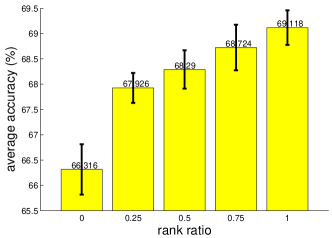
Figure 2: Illustrating how the CIFAR-$100$ classification accuracy changes when changing the rank of the idempotent matrix over a $20$-layer network. (changing $B$ when designing $\mathbf{P}_{\texttt{MR}}$). $0$ corresponds to that there is no skip-connection.

Training. We use the SGD algorithm with the Nesterov momentum to train all the networks for $300$ epochs on CIFAR-$10$/CIFAR-$100$ and $40$ epochs on SVHN, both with a total mini-batch size $64$. The initial learning rate is set to $0.1$, and is divided by $10$ at $1/2$ and $3/4$ of the total number of training epochs. Following residual networks [6], the weight decay is $0.0001$, the momentum is $0.9$, and the weights are initialized as in residual networks [6]. Our implementation is based on Keras and TensorFlow [1].

4.3 Results

Single-branch. We compare four skip-connections: Identity transformation, Idempotent-CMR, Orthogonal-TP and Orthogonal-Random. To form the idempotent matrix for Idempotent-CMR, we set $B$ to be the number of the channels, i.e., $\mathbf{P}_{{\texttt{MR}}}$ is a matrix with all entries being $\frac{1}{B}$. We do not evaluate Idempotent-MR because in this case its rank is only $1$, whose performance is expected to be low. In general, idempotent transformations with lower ranks perform worse than those with higher ranks. This is empirically verified in Figure 2.

Table 1 shows the results over networks of depth $20$ and $56$, containing $9$ and $27$ building blocks, respectively. One can see that the results with idempotent transformations and orthogonal transformations are similar to those with identity transformations: empirically demonstrating that idempotent transformations and orthogonal transformations improve information flow.

Table 1: Comparing classification accuracies of identity transformations, idempotent transformations, and orthogonal transformations for single-branch regular connections. $a+b$: $a$ is the average accuracy over five runs and $b$ is the standard deviation.

Depth	Mapping	Width	Accuracy
			CIFAR-$10$	CIFAR-$100$	SVHN
20	Identity	16,32,64	$92.468\pm 0.171$	$\mathbf{69.118\pm 0.341}$	$97.574\pm 0.109$
	Idempotent-CMR	16,32,64	$92.580\pm 0.088$	$69.048\pm 0.545$	$97.570\pm 0.056$
	Orthogonal-TP	16,32,64	$\mathbf{92.628\pm 0.158}$	$69.016\pm 0.509$	$\mathbf{97.616\pm 0.068}$
	Orthogonal-Random	16,32,64	$92.598\pm 0.097$	$68.716\pm 0.305$	$97.548\pm 0.087$
56	Identity	16,32,64	$94.396\pm 0.200$	$\mathbf{73.410\pm 0.350}$	$97.794\pm 0.083$
	Idempotent-CMR	16,32,64	$\mathbf{94.452\pm 0.267}$	$73.058\pm 0.210$	$\mathbf{97.794\pm 0.075}$
	Orthogonal-TP	16,32,64	$94.316\pm 0.299$	$73.352\pm 0.312$	$97.778\pm 0.081$
	Orthogonal-Random	16,32,64	$94.400\pm 0.206$	$73.288\pm 0.209$	$97.774\pm 0.059$

Table 2: Comparing classification accuracies for multiple-branch regular connections. The width of each branch is the same and the total width is described in the table.

Depth	Mapping	Width	Accuracy
			CIFAR-$10$	CIFAR-$100$	SVHN
20	Identity	32,64,128	$91.416\pm 0.308$	$67.002\pm 0.153$	$97.454\pm 0.095$
	Idempotent-CMR	32,64,128	$92.186\pm 0.238$	$68.520\pm 0.328$	$97.542\pm 0.040$
	Idempotent-MR	32,64,128	$92.454\pm 0.101$	$\mathbf{69.067\pm 0.242}$	$\mathbf{97.594\pm 0.051}$
	Orthogonal-TP	32,64,128	$\mathbf{92.538\pm 0.256}$	$69.044\pm 0.439$	$97.546\pm 0.058$
	Orthogonal-Random	32,64,128	$92.526\pm 0.147$	$68.668\pm 0.432$	$97.568\pm 0.025$
32	Identity	32,64,128	$-$	$68.158\pm 0.119$	$-$
	Idempotent-CMR	32,64,128	$-$	$70.372\pm 0.419$	$-$
	Idempotent-MR	32,64,128	$-$	$\mathbf{70.942\pm 0.331}$	$-$
	Orthogonal-TP	32,64,128	$-$	$70.786\pm 0.370$	$-$
	Orthogonal-Random	32,64,128	$-$	$70.926\pm 0.307$	$-$
56	Identity	32,64,128	$92.502\pm 0.224$	$69.524\pm 0.346$	$97.616\pm 0.102$
	Idempotent-CMR	32,64,128	$93.724\mp 0.135$	$72.192\pm 0.304$	$97.766\pm 0.102$
	Idempotent-MR	32,64,128	$93.858\pm 0.136$	$72.444\pm 0.143$	$\mathbf{97.816\pm 0.069}$
	Orthogonal-TP	32,64,128	$93.780\pm 0.289$	$\mathbf{72.716\pm 0.314}$	$97.724\pm 0.079$
	Orthogonal-Random	32,64,128	$\mathbf{93.886\pm 0.125}$	$72.476\pm 0.264$	$97.784\pm 0.052$
110	Identity	32,64,128	$-$	$71.112\pm 0.375$	$-$
	Idempotent-CMR	32,64,128	$-$	$73.822\pm 0.483$	$-$
	Idempotent-MR	32,64,128	$-$	$73.584\pm 0.039$	$-$
	Orthogonal-TP	32,64,128	$-$	$74.086\pm 0.333$	$-$
	Orthogonal-Random	32,64,128	$-$	$74.010\pm 0.299$	$-$

Four-branch. We compare the results over the networks, where each regular connection consists of four branches. The results are shown in Table 2. One can see that the idempotent and orthogonal transformations perform better than identity transformations. The reason is that compared to identity transformations, the designed idempotent and orthogonal transformations introduce interactions across the four branches.

Depth-wise. We evaluate the performance over extreme multi-branch networks: depth-wise networks, where each branch only contains a single channel. Table 3 shows the results. One can see that the comparison is consistent to the $4$-branch case.

Table 3: Comparing classification accuracies for depth-wise networks.

Depth	Mapping	Width	Accuracy
			CIFAR-$10$	CIFAR-$100$	SVHN
20	Identity	64, 128,256	$83.306\pm 0.243$	$58.388\pm 0.303$	$93.938\pm 0.138$
	Idempotent-CMR	64,128,256	$84.990\pm 0.389$	$\mathbf{60.360\pm 0.260}$	$95.488\pm 0.261$
	Orthogonal-TP	64,128,256	$\mathbf{85.456\pm 0.270}$	$58.828\pm 0.225$	$\mathbf{95.870\pm 0.065}$
	Orthogonal-Random	64,128,256	$84.800\pm 0.555$	$58.262\pm 0.415$	$95.816\pm 0.079$
56	Identity	64,128,256	$85.048\pm 0.354$	$60.242\pm 0.443$	$94.938\pm 0.099$
	Idempotent-CMR	64,128,256	$87.658\pm 0.217$	$\mathbf{63.068\pm 0.396}$	$96.818\pm 0.026$
	Orthogonal-TP	64,128,256	$87.932\pm 0.246$	$62.836\pm 0.465$	$\mathbf{97.134\pm 0.027}$
	Orthogonal-Random	64,128,256	$\mathbf{88.218\pm 0.207}$	$62.152\pm 0.312$	$97.058\pm 0.055$

5 Conclusions

We introduce two linear transformations, orthogonal and idempotent transformations, which, we show theoretically and empirically, behave like identity transformations, improving information flow and easing the training. One interesting point is that the success stems from feature and gradient reuse through the express way composed of skip-connections, for maintaining the information during flow and eliminating the gradient vanishing problem.

References

- [1] Martín Abadi, Ashish Agarwal, Paul Barham, Eugene Brevdo, Zhifeng Chen, Craig Citro, Gregory S. Corrado, Andy Davis, Jeffrey Dean, Matthieu Devin, Sanjay Ghemawat, Ian J. Goodfellow, Andrew Harp, Geoffrey Irving, Michael Isard, Yangqing Jia, Rafal Józefowicz, Lukasz Kaiser, Manjunath Kudlur, Josh Levenberg, Dan Mané, Rajat Monga, Sherry Moore, Derek Gordon Murray, Chris Olah, Mike Schuster, Jonathon Shlens, Benoit Steiner, Ilya Sutskever, Kunal Talwar, Paul A. Tucker, Vincent Vanhoucke, Vijay Vasudevan, Fernanda B. Viégas, Oriol Vinyals, Pete Warden, Martin Wattenberg, Martin Wicke, Yuan Yu, and Xiaoqiang Zheng. Tensorflow: Large-scale machine learning on heterogeneous distributed systems. CoRR, abs/1603.04467, 2016.
- [2] Masoud Abdi and Saeid Nahavandi. Multi-residual networks. CoRR, abs/1609.05672, 2016.
- [3] Anonymous. Deep convolutional neural networks with merge-and-run mappings. Under review.
- [4] Djork-Arné Clevert, Thomas Unterthiner, and Sepp Hochreiter. Fast and accurate deep network learning by exponential linear units (elus). arXiv preprint arXiv:1511.07289, 2015.
- [5] Xavier Glorot and Yoshua Bengio. Understanding the difficulty of training deep feedforward neural networks. In Aistats, volume 9, pages 249–256, 2010.
- [6] Kaiming He, Xiangyu Zhang, Shaoqing Ren, and Jian Sun. Delving deep into rectifiers: Surpassing human-level performance on imagenet classification. In ICCV, pages 1026–1034. IEEE Computer Society, 2015.
- [7] Kaiming He, Xiangyu Zhang, Shaoqing Ren, and Jian Sun. Deep residual learning for image recognition. In CVPR, pages 770–778. IEEE Computer Society, 2016.
- [8] Kaiming He, Xiangyu Zhang, Shaoqing Ren, and Jian Sun. Identity mappings in deep residual networks. In European Conference on Computer Vision, pages 630–645. Springer, 2016.
- [9] Gao Huang, Zhuang Liu, and Kilian Q. Weinberger. Densely connected convolutional networks. CoRR, abs/1608.06993, 2016.
- [10] Gao Huang, Yu Sun, Zhuang Liu, Daniel Sedra, and Kilian Q Weinberger. Deep networks with stochastic depth. In European Conference on Computer Vision, pages 646–661. Springer, 2016.
- [11] Sergey Ioffe and Christian Szegedy. Batch normalization: Accelerating deep network training by reducing internal covariate shift. arXiv preprint arXiv:1502.03167, 2015.
- [12] Alex Krizhevsky. Learning multiple layers of features from tiny images. Technical report, 2009.
- [13] Alex Krizhevsky, Ilya Sutskever, and Geoffrey E. Hinton. Imagenet classification with deep convolutional neural networks. In Peter L. Bartlett, Fernando C. N. Pereira, Christopher J. C. Burges, Léon Bottou, and Kilian Q. Weinberger, editors, NIPS, pages 1106–1114, 2012.
- [14] Gustav Larsson, Michael Maire, and Gregory Shakhnarovich. Fractalnet: Ultra-deep neural networks without residuals. CoRR, abs/1605.07648, 2016.
- [15] Chen-Yu Lee, Saining Xie, Patrick W. Gallagher, Zhengyou Zhang, and Zhuowen Tu. Deeply-supervised nets. In Guy Lebanon and S. V. N. Vishwanathan, editors, AISTATS, volume 38 of JMLR Workshop and Conference Proceedings. JMLR.org, 2015.
- [16] Min Lin, Qiang Chen, and Shuicheng Yan. Network in network. CoRR, abs/1312.4400, 2013.
- [17] Dmytro Mishkin and Jiri Matas. All you need is a good init. arXiv preprint arXiv:1511.06422, 2015.
- [18] Vinod Nair and Geoffrey E Hinton. Rectified linear units improve restricted boltzmann machines. In Proceedings of the 27th international conference on machine learning (ICML-10), pages 807–814, 2010.
- [19] Behnam Neyshabur, Ruslan R Salakhutdinov, and Nati Srebro. Path-sgd: Path-normalized optimization in deep neural networks. In Advances in Neural Information Processing Systems, pages 2422–2430, 2015.
- [20] Adriana Romero, Nicolas Ballas, Samira Ebrahimi Kahou, Antoine Chassang, Carlo Gatta, and Yoshua Bengio. Fitnets: Hints for thin deep nets. CoRR, abs/1412.6550, 2014.
- [21] Karen Simonyan and Andrew Zisserman. Very deep convolutional networks for large-scale image recognition. CoRR, abs/1409.1556, 2014.
- [22] Rupesh K Srivastava, Klaus Greff, and Jürgen Schmidhuber. Training very deep networks. In Advances in neural information processing systems, pages 2377–2385, 2015.
- [23] Christian Szegedy, Wei Liu, Yangqing Jia, Pierre Sermanet, Scott Reed, Dragomir Anguelov, Dumitru Erhan, Vincent Vanhoucke, and Andrew Rabinovich. Going deeper with convolutions. In Proceedings of the IEEE Conference on Computer Vision and Pattern Recognition, pages 1–9, 2015.
- [24] Sasha Targ, Diogo Almeida, and Kevin Lyman. Resnet in resnet: Generalizing residual architectures. CoRR, abs/1603.08029, 2016.
- [25] Antonio Torralba, Robert Fergus, and William T. Freeman. 80 million tiny images: A large data set for nonparametric object and scene recognition. IEEE Trans. Pattern Anal. Mach. Intell., 30(11):1958–1970, 2008.
- [26] Jingdong Wang, Zhen Wei, Ting Zhang, and Wenjun Zeng. Deeply-fused nets. CoRR, abs/1605.07716, 2016.
- [27] Saining Xie, Ross B. Girshick, Piotr Dollár, Zhuowen Tu, and Kaiming He. Aggregated residual transformations for deep neural networks. CoRR, abs/1611.05431, 2016.
- [28] Liming Zhao, Jingdong Wang, Xi Li, Zhuowen Tu, and Wenjun Zeng. On the connection of deep fusion to ensembling. CoRR, abs/1611.07718, 2016.