MISO in Ultra-Dense Networks: Balancing the Tradeoff between User and System Performance

Abstract

With over-deployed network infrastructures, network densification is shown to hinder the improvement of user experience and system performance. In this paper, we adopt multi-antenna techniques to overcome the bottleneck and investigate the performance of single-user beamforming, an effective method to enhance desired signal power, in small cell networks from the perspective of user coverage probability (CP) and network spatial throughput (ST). Pessimistically, it is proved that, even when multi-antenna techniques are applied, both CP and ST would be degraded and even asymptotically diminish to zero with the increasing base station (BS) density. Moreover, the results also reveal that the increase of ST is at the expense of the degradation of CP. Therefore, to balance the tradeoff between user and system performance, we further study the critical density, under which ST could be maximized under the CP constraint. Accordingly, the impact of key system parameters on critical density is quantified via the derived closed-form expression. Especially, the critical density is shown to be inversely proportional to the square of antenna height difference between BSs and users. Meanwhile, single-user beamforming, albeit incapable of improving CP and ST scaling laws, is shown to significantly increase the critical density, compared to the single-antenna regime.

I Introduction

Among the appealing approaches to fulfill the unprecedented capacity goals of the future wireless networks, network densification is shown to be the one with the greatest potential [1]. The basic principle behind network densification is to deploy base stations (BSs) or access points (APs) with smaller coverage to enable local spectrum reuse [2, 3]. As such, mobile users are served with short-distance transmission links, thereby facilitating enormous spectrum reuse gain and enhancing network capacity. The benefits of network densification are substantially verified via analytical results from academia [4, 5, 6, 7] and experimental results from industries [8, 9]. Remarkably, it is shown that over 1000-fold network capacity gain can be harvested by deploying hundreds of self-organizing small cells into one macro-cell, as compared to the macro-only case [8]. Despite the merits, however, the results show that network capacity starts to diminish when the number of small cells is sufficiently large in ultra-dense networks (UDN) [6, 7], in which short-distance transmissions are more likely to occur and accordingly inter-cell interference dominates the system performance. For this reason, the limitation of network densification remains to be fully explored.

I-A Related Work

The research on how network densification impacts the capacity of wireless networks has received extensive attention in the literature. In [4, 5], inspiring results have been obtained, showing that network capacity can be sustainably increased through deploying sufficient number of BSs in both single- and multi-tier networks. Nevertheless, the analysis in [4, 5] is made based on the premise that only non-line-of-sight (NLOS) paths exist between the transmitters (Tx’s) and the intended receivers (Rx’s). Due to the shorter transmission distance in dense BS deployment, line-of-sight (LOS) paths are more likely to appear as well. On this account, authors in [10, 6, 7] made attempts to investigate the impact of LOS/NLOS transmissions on the performance of downlink cellular networks. Particularly, it has been reported that the user coverage probability (CP) is degraded by network over-densification and, more importantly, network spatial throughput (ST) grows sublinearly or even decreases with the growing BS density [6, 7, 11].

In the aforementioned research, the 2-D distance is used to approximate the distance between the antennas of Tx’s and Rx’s. In sparsely deployed networks where Tx’s and Rx’s are far from each other, such approximation is of high accuracy and thus valid. When Tx’s and Rx’s are in proximity, however, it is apparent that the approximation will lose accuracy. Considering more practical cases, authors in [12] have investigated the performance of UDN in 3-D scenarios. Meanwhile, the impact of antenna height difference (AHD) between Tx’s and Rx’s has been examined in [13, 14]. In particular, the results in [13] indicate that, considering the existence of AHD, network capacity would even diminish to be zero when the density of deployed BSs in UDN approaches infinity. Nevertheless, as the obtained results are in complicated form, it fails to directly characterize how network performance is affected by AHD under a reasonable BS deployment density.

Intuitively, the main contributing factor that ruins the benefits of network densification is the inter-cell interference, which is likely to overwhelm the desired signal power when LOS paths exist between interfering BSs and the intended downlink user. Especially, when the density of elevated BSs further increases, more interfering BSs would have LOS paths to the intended user, thereby degrading network capacity. In this light, how to enhance desired signal power and mitigate interference is of utmost importance in UDN. Recently, a number of efficient interference management approaches have been tailored to tackle the interference in UDN [15, 16, 17]. For instance, an interference-separation clustering scheme has been designed for UDN in [15], aided by which inter-cluster interference could be effectively avoided through BS coordination. Besides, the combination of resource allocation and interference alignment has been studied to mitigate interference in UDN [16]. Nevertheless, the complexity of these methods cannot be kept at a reasonably low level, since most of them are run in a centralized manner. Worsestill, the required overhead to implement these methods would unboundedly increase with the network density, which may conversely ruin their potential benefits. Instead of alleviating overwhelming interference, increasing the desired signal power may serve as a promising alternative to enhance the system performance in UDN as well. For instance, authors in [18] evaluate the performance of cooperative transmissions in UDN. However, the results indicate that user spectral efficiency can hardly be improved by non-coherent joint transmission, whereas the spectral efficiency gain brought by coherent joint transmission is considerably dependent on channel models and system parameter settings. Therefore, more effective schemes are to be developed to enhance the performance of UDN.

In addition to the above discussion, it should be noted that more attentions have been paid on evaluating and improving the system-wide performance of UDN in most of the existing researches [10, 6, 19, 11, 13, 14]. Evidently, the quality of service (QoS) of users is an important indicator to the performance of UDN as well. Nonetheless, it is shown in [6] that the user CP could only reach 0.2 in UDN under 10dB decoding threshold and would even decrease with the growing BS density, which is typically deemed unacceptable in practice. Moreover, it is shown from [6] that the improvement of system performance (e.g., network ST) is at the cost of the deterioration of user performance (e.g., CP). For the above reason, it is crucial to improve the QoS of users and balance the tradeoff between user and network performance.

I-B Outcomes and Main Contribution

In this paper, using the tools of stochastic geometry, we investigate the performance of small cell networks, in which multiple antennas are equipped on each elevated BS and single-user beamforming (SU-BF) is applied as the multi-antenna technique. In particular, we provide a tractable approach to analyze the CP (user performance) and ST (system performance) in the multi-antenna regime, considering the AHD between BSs and users. On this basis, the fundamental limitation of network densification could be revealed. The main contribution of this paper are summarized in the following:

• Impact of AHD on the performance of UDN. Considering the antennas of BSs and users are of different heights, both CP and ST are shown to be degraded by network over-densification. Meanwhile, besides capturing the influence of AHD in the $\lambda\rightarrow\infty$ regime [13], where $\lambda$ denotes the BS density, we quantify the impact of AHD on CP and ST. In particular, it is revealed that CP and ST would be exponentially decreased with the square of AHD under typical settings.

• CP and ST scaling laws under the multi-antenna case. We shed light on the essential influence of SU-BF on the performance of UDN by studying the CP and ST scaling laws. Notably, it is shown that $\mathrm{\mathsf{CP}}\sim e^{-\bar{\kappa}\lambda}$ and $\mathsf{ST}\sim\lambda e^{-\bar{\kappa}\lambda}$, where $\bar{\kappa}$ is a function of system parameters (excluding BS density). In other words, even when multi-antenna techniques are applied, network over-densification would totally drain the spectrum reuse gain and degrade both user and system performance.

• Balancing the tradeoff between user and system performance. While SU-BF fails to improve the CP and ST scaling behavior, we show that CP and ST could be significantly enhanced by SU-BF. More importantly, to guarantee the QoS of users, we further analyze the critical density that could maximize the network ST under the CP constraint. Specifically, closed-form expressions of the critical density are retrieved in typical cases, which capture the impact of key system parameters on critical density. The above results could provide helpful insights and guidelines towards the planning and deployment of future wireless networks.

For the remainder of this paper, we first present the system model in Section II, followed by a preliminary analysis under the single-antenna regime in Section III. Afterward, we investigate the performance of UDN when SU-BF is applied in Section IV, based on which the tradeoff study on CP and ST is performed. Finally, conclusion remarks are given in Section V.

II System Model

II-A Network Model

Consider a downlink small cell network (see Fig. 1), where BSs (with constant transmit power $P$) and downlink users are distributed in a two-dimension plane $\mathbb{R}^{2}$, in line with two independent homogeneous Poisson Point Processes (PPPs), $\Pi_{\mathrm{BS}}=\left\{\mathrm{BS}_{i}\left|\mathrm{BS}_{i}\in\mathbb{R}^{2}\right.\right\}$ and $\Pi_{\mathrm{U}}=\left\{\mathrm{U}_{j}\left|\mathrm{U}_{j}\in\mathbb{R}^{2}\right.\right\}$ $\left(i,\>j\in\mathbb{N}\right)$, respectively. Denote $\lambda$ and $\lambda_{\mathrm{U}}$ as the densities of BSs and downlink users, respectively. It is assumed that each multi-antenna BS is equipped with antennas of height $h_{\mathrm{T}}$, while each single-antenna downlink user is equipped with antenna of height $h_{\mathrm{R}}$. Denote $\Delta h=\left|h_{\mathrm{T}}-h_{\mathrm{R}}\right|>0$ as the AHD between BSs and users and $N_{\mathrm{a}}$ as the number of antennas equipped on each BS.

The nearest association rule is adopted, i.e., downlink users are associated with the geometrically nearest BSs. It is further assumed that the user density is sufficiently large such that all the BSs are connected and activated. In each time slot, each BS would randomly select one of the associated users to serve. Besides, a saturated data model is considered such that users always require data to download from the serving BSs.

Figure 1: Illustration of downlink small cell networks.

II-B Single-user Beamforming

Instead of multi-user beamforming, SU-BF is applied as the multi-antenna technique at each BS side to enhance user and system performance in dense small cell networks. The main reasons are explained as follows. For one BS, serving all connected users using multi-user beamforming would require accurate estimation of channel state information (CSI) from all served users, whereas imperfect CSI estimation would result in significant performance degradation. In contrast, SU-BF, which only requires the CSI from single user, is more favorable. Besides, coordination among adjacent BSs is not considered, since it is difficult to form the coordination cluster in UDN. Even when coordination cluster is determined, CSI estimation and exchange within the coordination cluster requires excessive overhead.

According to the above discussion, we denote the channel vector from $\mathrm{BS}_{i}$ to $\mathrm{U}_{j}$ as $\mathbf{h}_{\mathrm{U}_{j},\mathrm{BS}_{i}}=\left[h_{\mathrm{U}_{j},\mathrm{BS}_{i},1},h_{\mathrm{U}_{j},\mathrm{BS}_{i},2},\ldots,h_{\mathrm{U}_{j},\mathrm{BS}_{i},N_{\mathrm{a}}}\right]$ with each complex entry independently distributed as complex normal distribution with zero mean, i.e., $\mathcal{CN}\left(0,1\right)$, and denote the SU-BF precoder from $\mathrm{BS}_{i}$ to $\mathrm{U}_{j}$ as $\mathbf{v}_{\mathrm{U}_{j},\mathrm{BS}_{i}}$, which is a unit $1\times N_{\mathrm{a}}$ vector. If $s_{i}$ is the data symbol sent by $\mathrm{BS}_{i}$, the received signal of $\mathrm{U}_{0}$, which is served by $\mathrm{BS}_{0}$, is given by

$$y_{0}= s_{0}\mathbf{h}_{\mathrm{U}_{0},\mathrm{BS}_{0}}\mathbf{v}_{\mathrm{U}_{0},\mathrm{BS}_{0}}^{\mathrm{T}}l_{N}^{\frac{1}{2}}\left(\left\{\alpha_{n}\right\}_{n=0}^{N-1};d_{0}\right)+\underset{\tiny{\mathrm{BS}_{i}\in\tilde{\Pi}_{\mathrm{BS}}}}{\sum}s_{i}\mathbf{h}_{\mathrm{U}_{0},\mathrm{BS}_{i}}\mathbf{v}_{\mathrm{U}_{0},\mathrm{BS}_{i}}^{\mathrm{T}}l_{N}^{\frac{1}{2}}\left(\left\{\alpha_{n}\right\}_{n=0}^{N-1};d_{i}\right)+n_{0},$$ (1)

where $l_{N}\left(\left\{\alpha_{n}\right\}_{n=0}^{N-1};d_{i}\right)$ denotes the pathloss from $\mathrm{BS}_{i}$ to $\mathrm{U}_{0}$, $n_{0}$ denotes the additive Gaussian noise and $\tilde{\Pi}_{\mathrm{BS}}=\Pi_{\mathrm{BS}}\backslash\mathrm{BS}_{0}$. In (1), $d_{i}$ denotes the distance from the antenna of $\mathrm{BS}_{i}$ to that of $\mathrm{U}_{0}$ for notation simplicity. Therefore, if denoting $\left\|\mathrm{BS}_{i}-\mathrm{U}_{0}\right\|$ as the 2D distance from $\mathrm{BS}_{i}$ to $\mathrm{U}_{0}$, we have $d_{i}=\sqrt{\left\|\mathrm{BS}_{i}-\mathrm{U}_{0}\right\|^{2}+\Delta h^{2}}$, where the notation $\left\|\cdot\right\|$ denotes the Euclidean norm operation. The detail of $l_{N}\left(\left\{\alpha_{n}\right\}_{n=0}^{N-1};d_{i}\right)$ will be discussed later.

Assume that the CSI of the $\mathrm{BS}_{i}$-$\mathrm{U}_{i}$ pair could be accurately estimated. In consequence, applying SU-BF would contribute to $\left\|\mathbf{h}_{\mathrm{U}_{i},\mathrm{BS}_{i}}\mathbf{v}_{\mathrm{U}_{i},\mathrm{BS}_{i}}^{\mathrm{T}}\right\|\sim\chi_{2N_{\mathrm{a}}}^{2}$ and $\left\|\mathbf{h}_{\mathrm{U}_{i},\mathrm{BS}_{j}}\mathbf{v}_{\mathrm{U}_{i},\mathrm{BS}_{j}}^{\mathrm{T}}\right\|\sim\chi_{2}^{2}$ $\left(i\neq j\right)$ [21, 22]. For this reason, the signal-to-interference ratio (SIR) at $\mathrm{U}_{0}$ can be expressed as

$$\mathsf{SIR}_{\mathrm{U}_{0}}=P\left\|\mathbf{h}_{\mathrm{U}_{0},\mathrm{BS}_{0}}\mathbf{v}_{\mathrm{U}_{0},\mathrm{BS}_{0}}^{\mathrm{T}}\right\|^{2}l_{N}\left(\left\{\alpha_{n}\right\}_{n=0}^{N-1};d_{0}\right)/I_{\mathrm{IC}}$$ , (2)

where $I_{\mathrm{IC}}=\underset{\tiny{\mathrm{BS}_{i}\in\tilde{\Pi}_{\mathrm{BS}}}}{\sum}P\left\|\mathbf{h}_{\mathrm{U}_{0},\mathrm{BS}_{i}}\mathbf{v}_{\mathrm{U}_{0},\mathrm{BS}_{i}}^{\mathrm{T}}\right\|^{2}l_{N}\left(\left\{\alpha_{n}\right\}_{n=0}^{N-1};d_{i}\right)$ denotes the intercell interference. It is worth noting that the influence of noise on the user performance is neglected, as we consider the interference-limited regime in UDN, where intercell interference dominates the user and system performance.

II-C Pathloss Model

To comprehensively characterize the LOS and NLOS components of signals in UDN, a multi-slope pathloss model (MSPM) has been adopted as [6, 7]

$$l_{N}\left(\left\{\alpha_{n}\right\}_{n=0}^{N-1};x\right)=K_{n}x^{-\alpha_{n}},\>R_{n}\leq x<R_{n+1}$$ (3)

where $K_{0}=1$, $K_{n}=\prod_{i=1}^{n}R_{i}^{\alpha_{i}-\alpha_{i-1}}$ $\left(n\geq 1\right)$, $0=R_{0}<R_{1}<\cdots<R_{N}=\infty$ and $0\leq\alpha_{0}\leq\alpha_{1}\leq\cdots\leq\alpha_{N-1}$ ($\alpha_{N-1}>2$ for practical concerns [6]).

From (3), it follows that different pathloss exponents are used to characterize the attenuation rates of signal power within different regions. As a typical example, when $N=2$, MSPM degenerates into the dual-slope pathloss model (DSPM) [6, 12]

$$l_{2}\left(\left\{\alpha_{n}\right\}_{n=0}^{1};x\right)=K_{n}x^{-\alpha_{n}},\>R_{n}\leq x<R_{n+1}$$ (4)

where $K_{0}=1$ and $K_{1}=R_{1}^{\alpha_{1}-\alpha_{0}}$. The DSPM in (4) is applied when an LOS path and a ground-reflected path exist between Tx and the intended Rx. As such, signal power attenuates slowly (with rate $\alpha_{0}$) within a corner distance $R_{1}$, while attenuates much more quickly (with rate $\alpha_{1}$) with distance out of $R_{1}$. When $N=1$, MSPM further degenerates into the most widely used single-slope pathloss model (SSPM) [4, 12]

$$l_{1}\left(\alpha_{0};x\right)=x^{-\alpha_{0}},\>x\in\left[0,\infty\right).$$ (5)

II-D Performance Metrics

We adopt CP and ST to reflect user and system performance, respectively. To be specific, following the SIR at $\mathrm{U}_{0}$ in (2), CP is defined as

$$\mathsf{CP}\left(\lambda\right)=\mathbb{P}\left\{\mathsf{SIR}_{\mathrm{U}_{0}}>\tau\right\},$$ (6)

where $\tau$ denotes the decoding threshold. Based on CP in (6), we further define network ST as [6, 12]

$$\mathsf{ST}\left(\lambda\right)=\lambda\mathbb{P}\left\{\mathsf{SIR}_{\mathrm{U}_{0}}>\tau\right\}\log_{2}\left(1+\tau\right),\>\left[\mathrm{bits}/\left(\mathrm{s\cdot Hz\cdot m^{2}}\right)\right]$$ (7)

which could characterize the number of bits that are successfully conveyed over unit time, frequency and area.

Notation: In the following, the notations $\mathsf{CP}_{N}^{\mathrm{S}}\left(\lambda\right)$ (resp. $\mathsf{ST}_{N}^{\mathrm{S}}\left(\lambda\right)$) and $\mathsf{CP}_{N}^{\mathrm{M}}\left(\lambda\right)$ (resp. $\mathsf{ST}_{N}^{\mathrm{M}}\left(\lambda\right)$) will be used. The superscript ’S’ denotes SISO system, while the superscript ’M’ denotes MISO system. The subscript $N$ denotes the number of slopes in MSPM. If ${}_{2}F_{1}\left(\cdot,\cdot,\cdot,\cdot\right)$ is defined as the standard Gaussian hypergeometric function, denote $\omega_{1}\left(x,y\right)=$ ${}_{2}F_{1}\left(1,1-\frac{2}{y},2-\frac{2}{y},-x\right)$, $\omega_{2}\left(x,y\right)=$ ${}_{2}F_{1}\left(1,\frac{2}{y},1+\frac{2}{y},-x\right)$ and $\delta\left(x,y\right)=\frac{2x\omega_{1}\left(x,y\right)}{y-2}$ in the rest of the paper. Besides, we use $l_{N}\left(x\right)$ as a substitution of $l_{N}\left(\left\{\alpha_{n}\right\}_{n=0}^{N-1};x\right)$ for notation simplicity.

III Preliminary Analysis

In this section, we provide preliminary analysis of CP and ST under MSPM when single antenna is equipped by each BS. The purpose is to lay the foundation for the analysis of multi-antenna case in Section IV.

III-A CP and ST in SISO system

When each BS is equipped with one antenna, no precoder is to be designed and, accordingly, the SIR at $\mathrm{U}_{0}$ in (2) would degenerate into

$$\mathsf{SIR}_{\mathrm{U}_{0}}^{\mathrm{S}}=P\left\|h_{\mathrm{U}_{0},\mathrm{BS}_{0}}\right\|^{2}l_{N}\left(\left\{\alpha_{n}\right\}_{n=0}^{N-1};d_{0}\right) /I_{\mathrm{IC}}^{\mathrm{S}},$$ (8)

where $I_{\mathrm{IC}}^{\mathrm{S}}=\underset{\tiny{\mathrm{BS}_{i}\in\tilde{\Pi}_{\mathrm{BS}}}}{\sum}P\left\|h_{\mathrm{U}_{0},\mathrm{BS}_{i}}\right\|^{2}l_{N}\left(\left\{\alpha_{n}\right\}_{n=0}^{N-1};d_{i}\right)$ denotes the intercell interference in the SISO system and $h_{\mathrm{U}_{0},\mathrm{BS}_{i}}$ denotes the channel from $\mathrm{BS}_{i}$ to $\mathrm{U}_{0}$.

In practice, when LOS path appears between Tx and the intended Rx, $h_{\mathrm{U}_{0},\mathrm{BS}_{i}}$ is more likely to follow complex normal distribution with non-zero mean (Rice fading), which is inconsistent with the $h_{\mathrm{U}_{0},\mathrm{BS}_{i}}\sim\mathcal{CN}\left(0,1\right)$ (Rayleigh fading) assumption in Section II-B. Nevertheless, we have tested via the experiment that signal envelop still follows Rayleigh distribution when Tx’s and Rx’s are geometrically close enough (several meters to dozens of meters), since the signal strengths of LOS and NLOS components are comparable [23]. More importantly, as will be shown later, the assumption on small-scale fading, which is considered as the minor factor to influence the performance of UDN [24], would exert little impact on CP and ST scaling laws.

Following (8), we give the main results on CP and ST under MSPM in SISO systems in Proposition 1.

Proposition 1.

Considering the AHD between single-antenna BSs and downlink users, the ST in downlink small cell networks under MSPM in (3) is given by $\mathsf{ST}_{N}^{\mathrm{S}}\left(\lambda\right)=\lambda\mathsf{CP}_{N}^{\mathrm{S}}\left(\lambda\right)\log_{2}\left(1+\tau\right)$, where $\mathsf{CP}_{N}^{\mathrm{S}}\left(\lambda\right)$ is given by (9).

$$\mathsf{CP}_{N}^{\mathrm{S}}\left(\lambda\right)=\left\{\begin{array}[]{cc}\frac{1}{1+\delta\left(\tau,\alpha_{0}\right)}\exp\left(-\pi\lambda\delta\left(\tau,\alpha_{0}\right)\Delta h^{2}\right),&N=1\\ \stackrel{{\scriptstyle[}}{{n}}=0]{N-1}{\sum}\mathbb{E}_{r_{0}\in\left[R_{n},R_{n+1}\right)}\left\{\exp\left[-\pi\lambda\left(\bar{R}_{n+1}^{2}\omega_{2}\left(\frac{\bar{R}_{n+1}^{\alpha_{n}}}{\tau d_{0}^{\alpha_{n}}},\alpha_{n}\right)-d_{0}^{2}\omega_{2}\left(\tau^{-1},\alpha_{n}\right)\right.\right.\right.\\ +\left.\left.\left.\stackrel{{\scriptstyle[}}{{i}}=n+1]{N-1}{\sum}\left(\bar{R}_{i+1}^{2}\omega_{2}\left(\frac{\bar{R}_{i+1}^{\alpha_{i}}}{\tau K_{i}d_{0}^{\alpha_{n}}},\alpha_{i}\right)-\bar{R}_{i}^{2}\omega_{2}\left(\frac{\bar{R}_{i}^{\alpha_{i}}}{\tau K_{i}d_{0}^{\alpha_{n}}},\alpha_{i}\right)\right)\right)\right]\right\},&N>1\end{array}\right.$$ (9)

In (9), $d_{0}=\sqrt{r_{0}^{2}+\Delta h^{2}}$ and the probability density function (PDF) of $r_{0}$ is derived from the contact distribution [20]

$$f_{r_{0}}\left(x\right)=2\pi\lambda x\exp\left(-\pi\lambda x^{2}\right),\>x\geq 0.$$ (10)

Proof: Please refer to Appendix A-A.∎

Despite in complicated form, the results in Proposition 1 could provide a numerical approach to capture the influence of system parameters on CP and ST, under MSPM. Meanwhile, according to the special case in (9), where $N=1$, it follows that both CP and ST would exponentially decrease with $\Delta h^{2}$. In other words, if ignoring the impact of the AHD (i.e., $\Delta h=0$), the merits of network densification would be greatly over-estimated. In addition, when MSPM degenerates into DSPM, the results on CP and ST could be further simplified as follows.

Corollary 1.

Considering the AHD between single-antenna BSs and downlink users, the ST in downlink small cell networks under DSPM in (4) is given by $\mathsf{ST}_{2}^{\mathrm{S}}\left(\lambda\right)=\lambda\mathsf{CP}_{2}^{\mathrm{S}}\left(\lambda\right)\log_{2}\left(1+\tau\right)$, where

$$\mathsf{CP}_{2}^{\mathrm{S}}\left(\lambda\right)=\mathbb{E}_{r_{0}\in\left[0,R_{1}\right)}\left[e^{-\pi\lambda\left(\delta_{1}\left(\alpha_{0},d_{0},\tau,R_{1}\right)+\delta_{2}\left(\alpha_{0},\alpha_{1},d_{0},\tau,R_{1}\right)\right)}\right]+\frac{e^{-\pi\lambda R_{1}^{2}\left(1+\delta\left(\tau,\alpha_{1}\right)\right)}}{1+\delta\left(\tau,\alpha_{1}\right)}.$$ (11)

In (11), $d_{0}=\sqrt{r_{0}^{2}+\Delta h^{2}}$, $\delta_{1}\left(\alpha_{0},d_{0},\tau,R_{1}\right)=R_{1}^{2}\omega_{2}\left(\frac{R_{1}^{\alpha_{0}}}{\tau d_{0}^{\alpha_{0}}},\alpha_{0}\right)-d_{0}^{2}\omega_{2}\left(\frac{1}{\tau},\alpha_{0}\right)$, $\delta_{2}\left(\alpha_{0},\alpha_{1},d_{0},\tau,R_{1}\right)=\frac{2\tau d_{0}^{\alpha_{0}}R_{1}^{2-\alpha_{0}}}{\alpha_{1}-2}\omega_{1}\left(\frac{\tau d_{0}^{\alpha_{0}}}{R_{1}^{\alpha_{0}}},\alpha_{1}\right)$, $\delta\left(\tau,\alpha_{1}\right)=\frac{2\tau\omega_{1}\left(\tau,\alpha_{1}\right)}{\alpha_{1}-2}$ and the PDF of $r_{0}$ is given by (10).

Proof: The proof can be completed by setting $N=2$ in (9) with easy manipulation, and is thus omitted due to space limitation.∎

(a) CP.

(b) ST.

Figure 2: CP and ST varying with AHD $\Delta h$. For system settings, set $P=23$dBm and $\tau=10$dB. For SSPM, set $\alpha_{0}=4$. For DSPM, set $\alpha_{0}=2.5$, $\alpha_{1}=4$ and $R_{1}=10$m. Lines and markers denote numerical and simulation results, respectively, in this figure and the remaining figures in this paper.

Based on Proposition 1 and Corollary 1, we illustrate the impact of AHD on CP and network ST in detail. In particular, Fig. 2 plots the CP and ST as a function of $\Delta h$ under different BS densities. It is shown that both CP and ST would be degraded by $\Delta h$. This indicates that, although the existence of $\Delta h$ would weaken both desired and interference signal power, the decrease of the desired signal power overwhelms that of the interference signal powers. Meanwhile, it is shown that the impact of $\Delta h$ on CP and ST is significant under dense BS deployment. Hence, in dense wireless networks, where the user antenna heights are basically small, it is preferable to deploy small cell BSs with smaller antenna heights so as to ensure the user performance as well as system performance.

As shown in Fig. 2, it is evident that the existence of $\Delta h$ leads to the performance degradation of downlink small cell networks in terms of CP and ST, especially when BSs are densely deployed. Therefore, we intend to further explore the influence of $\Delta h$ on the scaling laws of CP and ST in the following.

III-B CP and ST scaling laws in SISO system

In this part, before investigating the CP and ST scaling laws, results on $\omega_{1}\left(x,y\right)$ are first given in the following lemma.

Lemma 1.

For $y>2$, $\omega_{1}\left(x,y\right)$ is a decreasing function of $x$.

Proof: Please refer to the proof for Lemma 1 in [11].∎

To study the CP and ST scaling laws, the definition, which describes the growth rate (or order) of a function, is further given in the following.

Definition 1 (Function Limiting Behavior).

Denote $g_{1}\left(x\right)$ and $g_{2}\left(x\right)$ as two functions defined on the subset of real numbers. We write $g_{1}\left(x\right)=\Omega\left(g_{2}\left(x\right)\right)$ if $\exists m>0$, $x_{0}$, $\forall x>x_{0}$, $m\left|g_{2}\left(x\right)\right|\leq\left|g_{1}\left(x\right)\right|$, and $g_{1}\left(x\right)=\mathcal{O}\left(g_{2}\left(x\right)\right)$ if $\exists m>0$, $x_{0}$, $\forall x>x_{0}$, $\left|g_{1}\left(x\right)\right|\leq m\left|g_{2}\left(x\right)\right|$.

Aided by Definition 1 and Proposition 1, we show the CP and ST scaling laws in Theorem 1.

Theorem 1 (CP and ST Scaling Laws in SISO System).

When AHD exists between single-antenna BSs and downlink users, CP and ST scale with BS density $\lambda$ as $\mathsf{CP}_{N}^{\mathrm{S}}\left(\lambda\right)\sim e^{-\kappa\lambda}$ and $\mathsf{ST}_{N}^{\mathrm{S}}\left(\lambda\right)\sim\lambda e^{-\kappa\lambda}$ ($\kappa$ is a constant), respectively.

Proof: Please refer to Appendix A-B.∎

It is shown from Theorem 1 that both user and system performance would be degraded when BS density is sufficiently large. This is essentially different from the results in [10, 6, 19, 7], where BSs and users are equipped with antennas of the identical heights and the impact of AHD has not been taken into account in the scaling law analysis. Before showing the difference, we give the definition on critical density to facilitate better understanding of ST scaling law.

Definition 2 (Critical density).

Critical density is defined as the BS density, which maximizes network ST. Beyond the critical density, network ST starts to diminish with the growing BS density.

The critical density in Definition 2 serves as a useful metric to reflect the maximal density of BSs that could be deployed without degrading network capacity. Therefore, it can be used to reveal the fundamental limitation of network densification under different system settings.

(a) CP.

(b) ST.

Figure 3: CP and ST varying with BS density $\lambda$. For system settings, set $P=23$dBm and $\tau=10$dB. For SSPM, set $\alpha_{0}=4$. For DSPM, set $\alpha_{0}=2.5$, $\alpha_{1}=4$ and $R_{1}=10$m. To reflect the impact of LOS paths on signal propagation, we set $\upsilon_{\mathrm{NC}}=1$ and $\upsilon_{\mathrm{DoF}}=12$ for Rice fading.

Fig. 3 shows the CP and ST as a function of BS density $\lambda$ under different $\Delta h$. It is shown in Fig. 3a that, when $\Delta h=0$m, CP almost keeps constant with the increasing $\lambda$ under SSPM, and slowly decreases with the increasing $\lambda$ under DSPM (compared to the DSPM case under $\Delta h>0$m). In consequence, network ST would linearly/sublinearly grow with $\lambda$, as shown in Fig. 3b. In contrast, both CP and ST asymptotically approach zero when $\lambda$ is sufficiently large under $\Delta h>0$m. In practice, AHD exists between BSs and downlink users, even when small cell BSs are densely deployed. Therefore, the results in Theorem 1 could shed light on the fundamental limitation of network densification.

To verify the validity of the scaling law analysis under Rayleigh fading, we also evaluate the performance of downlink networks under Rice fading via simulation results in Fig. 3. Specifically, the channel power gain under Rice fading channels follows the non-central chi-square distribution with non-centrality parameter $\upsilon_{\mathrm{NC}}$ and degrees of freedom $\upsilon_{\mathrm{DoF}}$. It can be seen from Fig. 3 that, although gaps exist between the results under Rice and Rayleigh fadings, it is apparent that the CP and ST scaling laws under Rice fading are identical as those under Rayleigh fading. Following the above analysis, we further investigate the impact of SU-BF on CP and ST.

IV Performance Analysis Under SU-BF

In this section, we evaluate the performance of SU-BF in downlink small cell networks especially when BSs are densely deployed. To this end, we first extend the results on CP (resp. ST) and CP scaling law (resp. ST scaling law) in the following.

IV-A CP and ST in multi-antenna case

When SU-BF is applied at the BS side, the SIR at the typical downlink user $\mathrm{U}_{0}$ is given by (2) in Section II-B. Aided by the preliminary analysis in Section III, CP and ST can be derived via easy extension in the following corollary.

Corollary 2.

When SU-BF is applied by each multi-antenna BS, the ST in downlink small cell networks under MSPM in (3) is given by $\mathsf{ST}_{N}^{\mathrm{M}}\left(\lambda\right)=\lambda\mathsf{CP}_{N}^{\mathrm{M}}\left(\lambda\right)\log_{2}\left(1+\tau\right)$, where

$$\mathsf{CP}_{N}^{\mathrm{M}}\left(\lambda\right)= \mathbb{E}\left[\stackrel{{\scriptstyle[}}{{k}}=0]{N_{\mathrm{a}}-1}{\sum}\frac{\left(-s\right)^{k}}{k!}\frac{\mathrm{d}^{k}}{\mathrm{d}s^{k}}\mathcal{L}_{I_{\mathrm{IC}}}\left(s\right)\left|{}_{s=\frac{\tau}{2Pl_{N}\left(d_{0}\right)}}\right.\right].$$ (12)

In (12), $\mathcal{L}_{I_{\mathrm{IC}}}\left(s\right)$ is the Laplace Transform of $I_{I_{\mathrm{IC}}}$ evaluated at $s=\frac{\tau}{2Pl_{N}\left(d_{0}\right)}$, which is given by

$$\mathcal{L}_{I_{\mathrm{IC}}}\left(s\right)= \exp\left(-2\pi\lambda\int_{d_{0}}^{\infty}x\left(1-\frac{1}{1+2sPl_{N}\left(x\right)}\right)\mathrm{d}x\right).$$

Proof: Please refer to Appendix A-C.∎

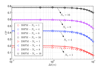
(a) CP.

(b) ST.

Figure 4: CP and ST varying with AHD $\Delta h$. For system settings, set $P=23$dBm and $\tau=10$dB. For SSPM, set $\alpha_{0}=4$. For DSPM, set $\alpha_{0}=2.5$, $\alpha_{1}=4$ and $R_{1}=10$m.

With the aid of Corollary 2, we illustrate how SU-BF enhances user and system performance in Fig. 4. In particular, Fig. 4 plots the CP and ST as a function of AHD $\Delta h$ when different number of antennas are equipped on each BS. It is observed that CP and ST could be greatly improved when SU-BF is applied. As an example, CP could only reach 0.2 in the single-antenna case under $\Delta h=1$m in Fig. 4a. When SU-BF is used with $N_{\mathrm{a}}=16$, however, CP could be increased to 0.78 under $\Delta h=1$m. Meanwhile, we see from Fig. 4 that CP and ST would be degraded more slowly with $\Delta h$ when more antennas are equipped on each BS. This also confirms the benefits of SU-BF in downlink small cell networks. In the following, we further investigate the performance of SU-BF in dense scenarios by studying CP and ST scaling laws.

Theorem 2 (CP and ST Scaling Laws in MISO System).

When SU-BF is applied, CP and ST scale with BS density $\lambda$ as $\mathsf{CP}_{N}^{\mathrm{M}}\left(\lambda\right)\sim e^{-\bar{\kappa}\lambda}$ and $\mathsf{ST}_{N}^{\mathrm{M}}\left(\lambda\right)\sim\lambda e^{-\bar{\kappa}\lambda}$ ($\bar{\kappa}$ is a constant), respectively, under MSPM.

Proof: Please refer to Appendix A-D.∎

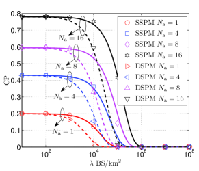
(a) CP.

(b) ST under SSPM.

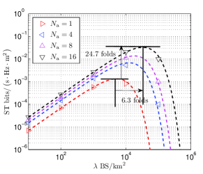
(c) ST under DSPM.

Figure 5: CP and ST varying with BS density $\lambda$. For system settings, set $P=23$dBm, $\tau=10$dB and $\Delta h$=2m. For SSPM, set $\alpha_{0}=4$. For DSPM, set $\alpha_{0}=2.5$, $\alpha_{1}=4$ and $R_{1}=10$m.

Theorem 2 indicates that network densification would ultimately degrade both user and system performance even when SU-BF is applied, which is somewhat pessimistic. Nevertheless, adopting SU-BF at the BS side indeed significantly enhances the desired signal power, which contributes to the improvement of user performance. We use the results in Fig. 5 to illustrate this, which plots the CP and ST as a function of BS density $\lambda$ under different $N_{\mathrm{a}}$. It is shown from Fig. 5a that, besides increasing CP, SU-BF could make CP degrade at a greater BS density under SSPM and DSPM. Meanwhile, it can be seen from Figs. 5b and 5c the maximal ST could be improved by 32.4 and 24.7 folds under SSPM and DSPM, respectively, when 16 antennas are equipped, compared to the single-antenna case. More importantly, the critical density could be considerably increased by SU-BF as well. It means that the bottleneck of network densification could be partially relieved with the application of SU-BF.

In addition, through the comparison of CP and ST scaling laws in Fig. 5, it is also observed that the improvement of system performance is at the cost of the degeneration of user experience. For instance, when $N_{\mathrm{a}}=16$, network ST grows with BS density at $1\times 10^{4}$BS/$\mathrm{km}^{2}$ (see Figs. 5b and 5c), under which CP already starts to diminish with $\lambda$ (see Fig. 5a). Therefore, besides ensuring the system performance, it is also critical to guarantee the user experience when planning the deployment of small cell networks.

IV-B Tradeoff between user and system performance

To balance the tradeoff between user and system performance, a CP requirement $\varepsilon$ is set to guarantee the QoS of downlink users as

$$\mathsf{CP}\left(\lambda\right)=\mathbb{P}\left\{\mathsf{SIR}_{\mathrm{U}_{0}}>\tau\right\}>\varepsilon.$$ (13)

It should be noted that, although the CP and ST scaling law analysis could be made using the lower and upper bounds in Theorem 2, it is still intractable to analytically obtain the closed-form expression of the critical density due to the complicated form of ST given in Corollary 2. As a substitution, we derive a simple but accurate approximation of CP in the following proposition.

Proposition 2.

When SU-BF is applied by each multi-antenna BS, the ST in downlink small cell networks under MSPM in (3) is approximated by $\tilde{\mathsf{ST}}_{N}^{\mathrm{M}}\left(\lambda\right)=\lambda\tilde{\mathsf{CP}}_{N}^{\mathrm{M}}\left(\lambda\right)\log_{2}\left(1+\tau\right)$, where $\tilde{\mathsf{CP}}_{N}^{\mathrm{M}}\left(\lambda\right)$ is given by (14).

$$\tilde{\mathsf{CP}}_{N}^{\mathrm{M}}\left(\lambda\right)=\left\{\begin{array}[]{cc}\frac{1}{1+\delta\left(\tau^{\dagger},\alpha_{0}\right)}\exp\left(-\pi\lambda\delta\left(\tau^{\dagger},\alpha_{0}\right)\Delta h^{2}\right),&N=1\\ \stackrel{{\scriptstyle[}}{{n}}=0]{N-1}{\sum}\mathbb{E}_{r_{0}\in\left[R_{n},R_{n+1}\right)}\left\{\exp\left[-\pi\lambda\left(\bar{R}_{n+1}^{2}\omega_{2}\left(\frac{\bar{R}_{n+1}^{\alpha_{n}}}{\tau^{\dagger}d_{0}^{\alpha_{n}}},\alpha_{n}\right)-d_{0}^{2}\omega_{2}\left(\frac{1}{\tau^{\dagger}},\alpha_{n}\right)\right.\right.\right.\\ +\left.\left.\left.\stackrel{{\scriptstyle[}}{{i}}=n+1]{N-1}{\sum}\left(\bar{R}_{i+1}^{2}\omega_{2}\left(\frac{\bar{R}_{i+1}^{\alpha_{i}}}{\tau^{\dagger}K_{i}d_{0}^{\alpha_{n}}},\alpha_{i}\right)-\bar{R}_{i}^{2}\omega_{2}\left(\frac{\bar{R}_{i}^{\alpha_{i}}}{\tau^{\dagger}K_{i}d_{0}^{\alpha_{n}}},\alpha_{i}\right)\right)\right)\right]\right\},&N>1\end{array}\right.$$ (14)

In (14), $\tau^{\dagger}=\frac{\tau}{N_{\mathrm{a}}}$, $d_{0}=\sqrt{r_{0}^{2}+\Delta h^{2}}$ and the PDF of $r_{0}$ is given by (10).

Proof: Please refer to Appendix A-E.∎

Remark 1.

The approximation in Proposition 2 is used to provide a tractable approach to evaluate the performance of dense small cell networks. The key is to use $\tilde{g}_{0}\sim\mathrm{Exp}\left(\frac{1}{2N_{\mathrm{a}}}\right)$ to approximate $\left\|\mathbf{h}_{\mathrm{U}_{0},\mathrm{BS}_{0}}\mathbf{v}_{\mathrm{U}_{0},\mathrm{BS}_{0}}^{\mathrm{T}}\right\|^{2}\sim\chi_{2N_{\mathrm{a}}}^{2}$. In particular, $\tilde{g}_{0}$ and $\left\|\mathbf{h}_{\mathrm{U}_{0},\mathrm{BS}_{0}}\mathbf{v}_{\mathrm{U}_{0},\mathrm{BS}_{0}}^{\mathrm{T}}\right\|^{2}$ share the identical mean. Although higher moments of $\tilde{g}_{0}$ and $\left\|\mathbf{h}_{\mathrm{U}_{0},\mathrm{BS}_{0}}\mathbf{v}_{\mathrm{U}_{0},\mathrm{BS}_{0}}^{\mathrm{T}}\right\|^{2}$ are close only when $N_{\mathrm{a}}$ is small, the impact of pathloss, which is a dominating factor to channel gain, on CP and ST significantly overwhelms that of small-scale fading when the distance from Tx’s to Rx’s is small in UDN. For the above reason, the approximation is reasonable.

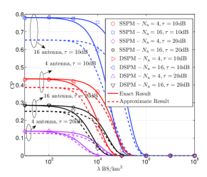
(a) CP.

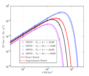
(b) ST under SSPM.

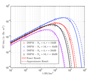
(c) ST under DSPM.

Figure 6: Exact and approximate CP/ST varying with BS density $\lambda$. For system settings, For system settings, set $P=23$dBm and $\Delta h$=2m. For SSPM, set $\alpha_{0}=4$. For DSPM, set $\alpha_{0}=2.5$, $\alpha_{1}=4$ and $R_{1}=10$m.

In Fig. 6, we examine the accuracy of the approximations in Proposition 2, where the comparison between the exact and approximate results on CP and ST is made. Fig. 6a indicates that there exist gaps between the exact and approximate results especially when BS density is small. Worsestill, the gaps would be enlarged when the number of antennas equipped on each BS is increased. However, the scaling behaviors of the approximate CP and ST are identical to those of the exact results. Meanwhile, the gaps are shown to be reduced when BS density becomes larger (see Figs. 6b and 6c). More importantly, the exact and approximate critical densities are almost identical. As the approximation is used to derive more simple and insightful results on the critical density, the above discussion is sufficient to validate the accuracy of the approximation in Proposition 2.

With the approximate results in Proposition 2, we then study the critical density with the CP requirement specified in (13). From (13), it is intuitive that whether or not the requirement could be satisfied primarily depends on the deployment density of BSs. However, as observed from Fig. 6a, even when BS density is small, the maximal CP that can be achieved only reaches 0.79 under $N_{\mathrm{a}}=16$ and $\tau=10$dB. This indicates that, besides BS density, other parameters such as pathloss exponents, decoding threshold, etc., impact whether the CP requirement could be met as well. In this light, we first analyze the necessary condition to acquire the CP requirement. Afterward, we derive the critical density, under which network ST can be maximized under the pre-set CP requirement.

IV-C Critical density under SSPM and DSPM

Aided by the approximation in Proposition 2, we first analyze the necessary condition, under which the CP requirement specified in (13) could be satisfied.

Theorem 3.

Under MSPM in (3), the necessary condition to satisfy the CP requirement in (13) is given by

$$\frac{2\tau^{\dagger}\omega_{1}\left(\tau^{\dagger},\alpha_{N-1}\right)}{\alpha_{N-1}-2}<\varepsilon^{-1}-1,$$ (15)

where $\tau^{\dagger}=\frac{\tau}{N_{\mathrm{a}}}$.

Proof: Please refer to Appendix A-F.∎

Theorem 3 provides a direct approach on how to reasonably adjust system parameters to meet the pre-set CP requirement of downlink users. For instance, it is easy to prove that $\psi_{N}\left(\tau,\alpha_{N-1},N_{\mathrm{a}}\right)=\frac{\tau}{N_{\mathrm{a}}}\omega_{1}\left(\frac{\tau}{N_{\mathrm{a}}},\alpha_{N-1}\right)$ in the left-hand-side of (15) is an increasing function of the decoding threshold $\tau$. Therefore, the CP requirement is less likely to be met with a greater $\tau$. Nevertheless, Theorem 3 indicates that increasing the number of antennas would directly relieve this. Specifically, following (15), increasing $N_{\mathrm{a}}$ is equivalent to lowering the decoding threshold $\tau$. Although the results in Theorem 3 are derived from the approximate results in Proposition 2, the benefits of applying multi-antenna techniques in UDN can be more directly revealed.

Aided by Theorem 3, we further investigate the critical BS density under two typical pathloss models, namely, SSPM in (5) and DSPM in (4), thereby providing helpful insights and guideline towards the deployment of dense small cell networks.

Corollary 3 (Critical Density under SSPM).

Under SSPM in (5), the critical BS density $\lambda_{1}^{\dagger}$, under which network ST is maximized without the CP constraint, is given by

$$\lambda_{1}^{\dagger}=\frac{\alpha_{0}-2}{2\pi\tau^{\dagger}\omega_{1}\left(\tau^{\dagger},\alpha_{0}\right)\Delta h^{2}},$$ (16)

where $\tau^{\dagger}=\frac{\tau}{N_{\mathrm{a}}}$. With the CP constraint $\varepsilon$, the critical BS density $\lambda_{1}^{*}$ is given by

$$\lambda_{1}^{*}=\max\left(\lambda_{1}^{\dagger}\ln\left[\varepsilon^{-1}\left(1+\frac{2\tau^{\dagger}\omega_{1}\left(\tau^{\dagger},\alpha_{0}\right)}{\alpha_{0}-2}\right)^{-1}\right],\lambda_{1}^{\dagger}\right).$$ (17)

Proof: Please refer to Appendix A-G.∎

Corollary 3 reveals the fundamental limitation of small cell networks by quantifying how many BSs could be deployed per unit area (critical density), and more importantly characterizes the impact of key system parameters on the critical density. For instance, as $\psi\left(\tau,\alpha_{0},N_{\mathrm{a}}\right)=\frac{\tau}{N_{\mathrm{a}}}\omega_{1}\left(\frac{\tau}{N_{\mathrm{a}}},\alpha_{0}\right)$ in the denominator of $\lambda_{1}^{*}$ and $\lambda_{1}^{\dagger}$ decreases with the increasing $N_{\mathrm{a}}$, the results indicate that increasing the number of antennas would result in an increase of the critical density.

Next, we further investigate the critical densities under DSPM in Corollary 4.

Corollary 4 (Critical Density under DSPM).

Under DSPM in (4), the critical BS density $\lambda_{2}^{\dagger}$, under which network ST is maximized without the CP constraint, is approximated as

$$\lambda_{2}^{\dagger}=\frac{1}{\pi\left[R_{1}^{2}\left(1+\delta\left(\tau^{\dagger},\alpha_{1}\right)\right)+\Delta h^{2}\delta\left(\tau^{\dagger},\alpha_{1}\right)\right]},$$ (18)

where $\tau^{\dagger}=\frac{\tau}{N_{\mathrm{a}}}$. With the CP constraint $\varepsilon$, the critical BS density $\lambda_{2}^{*}$ is approximated as

$$\lambda_{2}^{*}=\max\left(\lambda_{2}^{\dagger}\ln\left[\varepsilon^{-1}\left(1+\delta\left(\tau^{\dagger},\alpha_{1}\right)\right)^{-1}\right],\lambda_{2}^{\dagger}\right).$$ (19)

The approximations are of high accuracy when $R_{1}$ in (4) is large.

Proof: Please refer to Appendix A-H. ∎

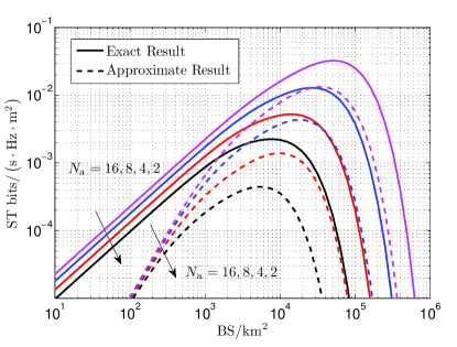
(a) ST under $R_{1}=10$m.

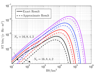
(b) ST under $R_{1}=50$m

Figure 7: Exact and approximate ST varying with BS density $\lambda$ under DSPM. For system settings, set $P=23$dBm, $\tau=0$dB and $\Delta h$=2m. For SSPM, set $\alpha_{0}=4$. For DSPM, set $\alpha_{0}=2.5$ and $\alpha_{1}=4$.

As indicated by Corollary 4, the approximation of critical densities are valid when the corner distance $R_{1}$ in (4) is large. We use the results in Fig. 7 to verify this. Figs. 7a and 7b plot the exact and approximate ST as a function of BS density under DSPM when $R_{1}=10$m and $R_{1}=50$m, respectively. Notably, it can be seen that the critical densities obtained via exact and approximate results are almost identical under the given settings. According to [25], $R_{1}\approx\frac{4h_{\mathrm{T}}h_{\mathrm{R}}f_{\mathrm{c}}}{c}$, where $f_{c}$ denotes the carrier frequency and $c=3\times 10^{8}$m/s denotes the light speed. Given $h_{\mathrm{T}}=2.5$m and $h_{\mathrm{R}}=1.5$m, $R_{1}$ basically ranges from several meters to dozens of meters under sub-6GHz and increases with $f_{c}$. For this reason, the approximations in Corollary 4 are reasonable in practice.

(a) Critical density under SSPM.

(b) Critical density under DSPM.

Figure 8: Critical densities $\lambda^{*}$ and $\lambda^{\dagger}$ varying with the AHD $\Delta h$. For system settings, set $P=23$dBm and $\tau=0$dB. For SSPM, set $\alpha_{0}=4$. For DSPM, set $\alpha_{0}=2.5$, $\alpha_{1}=4$ and $R_{1}=10$m. Note that $\varepsilon=0$ is equivalent to the case, where no CP requirement is considered.

It is also observed from Corollaries 3 and 4 that the critical densities would be decreased by the CP requirement $\varepsilon$ and AHD $\Delta h$. Especially, Fig. 8 shows the critical density as a function of $\Delta h$ under different $\varepsilon$. It is observed from Fig. 8a that the critical density is reduced by 5.8 and even 19.7 folds when $\varepsilon=0.8$ and $\varepsilon=0.9$, respectively, when $N_{\mathrm{a}}=16$ and $\Delta h=2$m under SSPM. Using the same system settings, the critical density is reduced by 6.1 and 21.7 folds, respectively, under DSPM as well. The results demonstrate that the CP requirement greatly limits the maximal BS deployment density. In addition, as critical density would increase inversely with $\Delta h^{2}$, the above results also reveal the essential influence of AHD on the BS deployment in downlink small cell networks. In particular, it indicates that a great $\Delta h$ would hinder the increase of ST in dense scenarios. From this perspective, it suggests that the antenna height of small cell BSs should be lowered, thereby facilitating the maximization of network ST while ensuring the QoS of downlink users.

V Conclusion

In this paper, we have explored the fundamental limits of network densification in downlink small cell networks when SU-BF serves as the multi-antenna transmission technique under a generalized multi-slope pathloss model. While incapable of improving the CP and ST scaling laws, the application of MISO is shown to significantly enhance user experience and system performance and even increase the critical density. Meanwhile, aided by the simple but accurate approximations, the influence of multi-antenna techniques on CP and ST could be explicitly revealed. In addition, it is observed that the CP of downlink users starts to diminish with the BS density when network ST is increased. Therefore, to strike a better balance between user and system performance, we have analyzed the critical density, under which network ST can be maximized with the pre-set CP requirement. The results could provide helpful guidance for the network deployment and application of network densification in future wireless networks.

Appendix A *

A-A Proof for Proposition 1

In the following, $H_{\mathrm{U}_{0},\mathrm{BS}_{i}}$ is used to replace $\left\|h_{\mathrm{U}_{0},\mathrm{BS}_{i}}\right\|^{2}$. Substituting (8) into (6), we have

$$\mathsf{CP}_{N}^{\mathrm{S}}\left(\lambda\right)\overset{\left(\mathrm{a}\right)}{=}\mathbb{P}\left\{H_{\mathrm{U}_{0},\mathrm{BS}_{0}}>s_{N}^{\mathrm{S}}I_{\mathrm{IC}}^{\mathrm{S}}\right\}=\mathbb{E}_{d_{0}}\left[e^{-2\pi\lambda\int_{d_{0}}^{\infty}x\left(1-\frac{1}{1+s_{N}^{\mathrm{S}}Pl_{N}\left(x\right)}\right)\mathrm{d}x}\right],$$ (20)

where $s_{N}^{\mathrm{S}}=\frac{\tau}{Pl_{N}\left(d_{0}\right)}$. For the derivation of step (a), please refer to (5) in [11] for detail.

Given $N=1$, it is straightforward to obtain $s_{1}^{\mathrm{S}}=\frac{\tau d_{0}^{\alpha_{0}}}{P}$ and

$$\mathsf{CP}_{1}^{\mathrm{S}}\left(\lambda\right)= \mathbb{E}_{d_{0}}\left[\exp\left(-\frac{2\pi\lambda\tau\omega_{1}\left(\tau,\alpha_{0}\right)}{\alpha-2}d_{0}^{2}\right)\right]=\mathbb{E}_{r_{0}}\left[\exp\left(-\frac{2\pi\lambda\tau\omega_{1}\left(\tau,\alpha_{0}\right)}{\alpha-2}\left(r_{0}^{2}+\Delta h^{2}\right)\right)\right]$$

$$\overset{\left(\mathrm{a}\right)}{=} \frac{1}{1+\delta\left(\tau,\alpha_{0}\right)}\exp\left(-\pi\lambda\bigtriangleup h^{2}\delta\left(\tau,\alpha_{0}\right)\right),$$ (21)

where (a) follows because the PDF of $r_{0}$ is given by (10).

Given $N>1$ and $d_{0}\in\left[\bar{R}_{n},\bar{R}_{n+1}\right)$ with $\bar{R}_{n}=\sqrt{r_{0}^{2}+R_{n}^{2}}$, $\int_{d_{0}}^{\infty}x^{k-1}\left(1-\frac{1}{1+s_{N}^{\mathrm{S}}Pl_{N}\left(x\right)}\right)\mathrm{d}x$ in (20) turns into $\int_{d_{0}}^{\infty}x\left(1-\frac{1}{1+s_{N}^{\mathrm{S}}Pl_{N}\left(x\right)}\right)\mathrm{d}x$

$$= \int_{d_{0}}^{\bar{R}_{n+1}}x\left(1-\frac{1}{1+\tau d_{0}^{\alpha_{n}}x^{-\alpha_{n}}}\right)\mathrm{d}x+\stackrel{{\scriptstyle[}}{{i}}=n+1]{N-1}{\sum}\int_{\bar{R}_{i}}^{\bar{R}_{i+1}}x\left(1-\frac{1}{1+\tau K_{i}d_{0}^{\alpha_{n}}x^{-\alpha_{i}}}\right)\mathrm{d}x$$

$$= \frac{1}{2}\left[\bar{R}_{n+1}^{2}\omega_{2}\left(\frac{\bar{R}_{n+1}^{\alpha_{n}}}{\tau d_{0}^{\alpha_{n}}},\alpha_{n}\right)-d_{0}^{2}\omega_{2}\left(\tau^{-1},\alpha_{n}\right)\right]+\stackrel{{\scriptstyle[}}{{i}}=n+1]{N-1}{\sum}\left[\frac{\bar{R}_{i+1}^{2}}{2}\omega_{2}\left(\frac{\bar{R}_{i+1}^{\alpha_{i}}}{\tau K_{i}d_{0}^{\alpha_{n}}},\alpha_{i}\right)-\frac{\bar{R}_{i}^{2}}{2}\omega_{2}\left(\frac{\bar{R}_{i}^{\alpha_{i}}}{\tau K_{i}d_{0}^{\alpha_{n}}},\alpha_{i}\right)\right].$$ (22)

According to (22), $\mathsf{CP}_{N}^{\mathrm{S}}\left(\lambda\right)$ $\left(N>1\right)$ could be obtained and hence the proof is completed.

A-B Proof for Theorem 1

From (9) in Proposition 1, the proof for the scaling laws of CP and ST under the SSPM is straightforward. Therefore, we focus on the proof for the case with $N>1$.

Given $N>1$, the CP in (9) can be expressed as $\mathsf{CP}_{N}^{\mathrm{S}}\left(\lambda\right)$

$$=\mathbb{E}_{r_{0}\in\left[R_{0},R_{N-1}\right)}\left[e^{-2\pi\lambda\int_{d_{0}}^{\infty}x\left(1-\frac{1}{1+s_{N}^{\mathrm{S}}Pl_{N}\left(x\right)}\right)\mathrm{d}x}\right]+\mathbb{E}_{r_{0}\in\left[R_{N-1},R_{N}\right)}\left[e^{-2\pi\lambda\int_{d_{0}}^{\infty}x\left(1-\frac{1}{1+s_{N}^{\mathrm{S}}Pl_{N}\left(x\right)}\right)\mathrm{d}x}\right].$$ (23)

Then, the following inequality holds true, i.e.,

$$\mathsf{CP}_{N}^{\mathrm{S}}\left(\lambda\right)> \mathbb{E}_{r_{0}\in\left[R_{N-1},R_{N}\right)}\left[e^{-2\pi\lambda\int_{d_{0}}^{\infty}x\left(1-\frac{1}{1+s_{N}^{\mathrm{S}}Pl_{N}\left(x\right)}\right)\mathrm{d}x}\right].$$ (24)

As $d_{0}=\sqrt{r_{0}^{2}+\Delta h^{2}}$, $\bar{R}_{N-1}=\sqrt{R_{N-1}^{2}+\Delta h^{2}}$ and $R_{N}=\infty$, when $d_{0}\in\left[\bar{R}_{N-1},\infty\right)$, $s_{N}^{\mathrm{S}}=\frac{\tau}{PK_{N-1}d_{0}^{-\alpha_{N-1}}}$ and $l_{N}\left(x\right)=K_{N-1}x^{-\alpha_{N-1}}$, the integral in (24) turns into

$$\int_{d_{0}}^{\infty}x\left(1-\frac{1}{1+\tau d_{0}^{\alpha_{N-1}}x^{-\alpha_{N-1}}}\right)\mathrm{d}x=\frac{\delta\left(\tau,\alpha_{N-1}\right)d_{0}^{2}}{2}=\frac{\delta\left(\tau,\alpha_{N-1}\right)}{2}\left(r_{0}^{2}+\Delta h^{2}\right),$$ (25)

where $\delta\left(\tau,\alpha_{N-1}\right)=\frac{2\tau\omega_{1}\left(\tau,\alpha_{N-1}\right)}{\alpha_{N-1}-2}$. Following (25), we derive the lower bound of $\mathsf{CP}_{N}^{\mathrm{S}}\left(\lambda\right)$ as

$$\mathsf{CP}_{N}^{\mathrm{S}}\left(\lambda\right)> \mathsf{CP}_{N-\mathrm{L}}^{\mathrm{\mathrm{S}}}\left(\lambda\right)=\mathbb{E}_{r_{0}\in\left[R_{N-1},\infty\right)}\left[e^{-\pi\lambda\delta\left(\tau,\alpha_{N-1}\right)\left(r_{0}^{2}+\Delta h^{2}\right)}\right]$$

$$= \frac{e^{-\pi\lambda\left[R_{N-1}^{2}+\delta\left(\tau,\alpha_{N-1}\right)\left(R_{N-1}^{2}+\Delta h^{2}\right)\right]}}{1+\delta\left(\tau,\alpha_{N-1}\right)}.$$ (26)

Therefore, it can be shown that $\exists\frac{1}{1+\delta\left(\tau,\alpha_{N-1}\right)}>0$, $\forall\lambda>0$,

$$\left|\mathsf{CP}_{N-\mathrm{L}}^{\mathrm{\mathrm{S}}}\left(\lambda\right)\right| \geq\frac{e^{-\pi\lambda\left[R_{N-1}^{2}+\delta\left(\tau,\alpha_{N-1}\right)\left(R_{N-1}^{2}+\Delta h^{2}\right)\right]}}{1+\delta\left(\tau,\alpha_{N-1}\right)}.$$ (27)

According to Definition 1, $\mathsf{CP}_{N-\mathrm{L}}^{\mathrm{\mathrm{S}}}=\Omega\left(e^{-\pi\lambda\left[R_{N-1}^{2}+\delta\left(\tau,\alpha_{N-1}\right)\left(R_{N-1}^{2}+\Delta h^{2}\right)\right]}\right)$ holds true.

In the following, we analyze the upper bound of $\mathsf{CP}_{N}^{\mathrm{S}}\left(\lambda\right)$. When $r_{0}\in\left[R_{n},R_{n+1}\right)$ or equivalently $d_{0}\in\left[\bar{R}_{n},\bar{R}_{n+1}\right)$ $\left(n=0,1,\ldots,N-2\right)$, $s_{N}^{\mathrm{S}}=\frac{\tau d_{0}^{\alpha_{n}}}{PK_{n}}$. As such, $\int_{d_{0}}^{\infty}x\left(1-\frac{1}{1+s_{N}^{\mathrm{S}}Pl_{N}\left(x\right)}\right)\mathrm{d}x$ in the first term of (23) can be manipulated as $\int_{d_{0}}^{\infty}x\left(1-\frac{1}{1+s_{N}^{\mathrm{S}}Pl_{N}\left(x\right)}\right)\mathrm{d}x$

$$\overset{\left(\mathrm{a}\right)}{>} \int_{\bar{R}_{N-1}}^{\infty}x\left(1-\frac{1}{1+\frac{\tau K_{N-1}}{K_{n}d_{0}^{-\alpha_{n}}}x^{-\alpha_{N-1}}}\right)\mathrm{d}x=\frac{\tau K_{N-1}\bar{R}_{N-1}^{2-\alpha_{N-1}}d_{0}^{\alpha_{n}}}{K_{n}\left(\alpha_{N-1}-2\right)}\omega_{1}\left(\frac{\tau K_{N-1}d_{0}^{\alpha_{n}}}{K_{n}R_{N-1}^{\alpha_{N-1}}},\alpha_{N-1}\right)$$

$$\overset{\left(\mathrm{b}\right)}{>} \frac{\tau K_{N-1}\bar{R}_{N-1}^{2-\alpha_{N-1}}\Delta h^{\alpha_{n}}}{K_{n}\left(\alpha_{N-1}-2\right)}\omega_{1}\left(\frac{\tau K_{N-1}}{K_{n}},\alpha_{N-1}\right)=q_{1}\left(n\right),$$ (28)

where (a) follows due to $d_{0}<\bar{R}_{N-1}$, and (b) follows because $d_{0}>\Delta h$, $d_{0}^{\alpha_{n}}<R_{N-1}^{\alpha_{N-1}}$ and $\omega_{1}\left(x,\alpha_{N-1}\right)$ is a decreasing function of $x$ (see Lemma 1). Using (28) and the PDF of $r_{0}$ in (10), we have $\mathbb{E}_{r_{0}\in\left[R_{0},R_{N-1}\right)}\left[e^{-2\pi\lambda\int_{d_{0}}^{\infty}x\left(1-\frac{1}{1+s_{N}^{\mathrm{S}}Pl_{N}\left(x\right)}\right)\mathrm{d}x}\right]$

$$< \stackrel{{\scriptstyle[}}{{n}}=0]{N-2}{\sum}\mathbb{E}_{r_{0}\in\left[R_{n},R_{n+1}\right)}\left[e^{-2\pi\lambda q_{1}\left(n\right)}\right]=\stackrel{{\scriptstyle[}}{{n}}=0]{N-2}{\sum}e^{-2\pi\lambda q_{1}\left(n\right)}\left(e^{-\pi\lambda R_{n}^{2}}-e^{-\pi\lambda R_{n+1}^{2}}\right).$$ (29)

When $r_{0}\in\left[R_{N-1},\infty\right)$, the second term of (23) is already given by $\mathsf{CP}_{N-\mathrm{L}}^{\mathrm{\mathrm{S}}}\left(\lambda\right)$ in (26). Hence, it is easy to obtain that

$$\mathsf{CP}_{N}^{\mathrm{\mathrm{S}}}\left(\lambda\right)< \stackrel{{\scriptstyle[}}{{n}}=0]{N-2}{\sum}e^{-2\pi\lambda q_{1}\left(n\right)}\left(e^{-\pi\lambda R_{n}^{2}}-e^{-\pi\lambda R_{n+1}^{2}}\right)+\mathsf{CP}_{N-\mathrm{L}}^{\mathrm{\mathrm{S}}}\left(\lambda\right)$$

$$< \stackrel{{\scriptstyle[}}{{n}}=0]{N-2}{\sum}e^{-2\pi\lambda q_{1}\left(n\right)}e^{-\pi\lambda R_{n}^{2}}+\mathsf{CP}_{N-\mathrm{L}}^{\mathrm{\mathrm{S}}}\left(\lambda\right)\overset{\left(\mathrm{a}\right)}{<}\stackrel{{\scriptstyle[}}{{n}}=0]{N-2}{\sum}e^{-2\pi\lambda q_{1}\left(n\right)}+e^{-\pi\lambda R_{N-1}^{2}}$$

$$= \mathsf{CP}_{N-\mathrm{U}}^{\mathrm{\mathrm{S}}}\left(\lambda\right).$$ (30)

where (a) follows because $e^{-\pi\lambda R_{n}^{2}}<1$ and it is direct to show $\mathsf{CP}_{N-\mathrm{L}}^{\mathrm{\mathrm{S}}}\left(\lambda\right)<e^{-\pi\lambda R_{N-1}^{2}}$. In (30), if $n\in\mathbb{C}$ $\left(\mathbb{C}=\left\{0,1,\ldots,N-2\right\}\right)$, which enables $2q_{1}\left(n\right)>R_{N-1}^{2}$, then the inequality $e^{-2\pi\lambda q_{1}\left(n\right)}<e^{-\pi\lambda R_{N-1}^{2}}$ holds. Thus, $\mathsf{CP}_{N-\mathrm{U}}^{\mathrm{\mathrm{S}}}\left(\lambda\right)$ in (30) turns into

$$\mathsf{CP}_{N-\mathrm{U}}^{\mathrm{\mathrm{S}}}\left(\lambda\right)=\stackrel{{\scriptstyle[}}{{n}}=0]{N-2}{\sum}e^{-2\pi\lambda q_{1}\left(n\right)}+e^{-\pi\lambda R_{N-1}^{2}}< Ne^{-\pi\lambda R_{N-1}^{2}},$$

which indicates that $\exists N>0$, $\forall\lambda>0$,

$$\left|\mathsf{CP}_{N-\mathrm{U}}^{\mathrm{\mathrm{S}}}\left(\lambda\right)\right|< Ne^{-\pi\lambda R_{N-1}^{2}}.$$ (31)

If $n\in\mathbb{C}^{\dagger}$ $\left(\mathbb{C}\subseteq\left\{0,1,\ldots,N-2\right\}\right)$, which enables $2q_{1}\left(n\right)\leq R_{N-1}^{2}$, then we denote $n=N^{\dagger}$, which makes $e^{-2\pi\lambda q_{1}\left(N^{\dagger}\right)}\geq e^{-2\pi\lambda q_{1}\left(n\right)}$ $\left(0\leq n\leq N-2\right)$. It is apparent that $e^{-2\pi\lambda q_{1}\left(N^{\dagger}\right)}\geq e^{-\pi\lambda R_{N-1}^{2}}$ holds as well. Thus, we have

$$\mathsf{CP}_{N-\mathrm{U}}^{\mathrm{\mathrm{S}}}\left(\lambda\right)=\stackrel{{\scriptstyle[}}{{n}}=0]{N-2}{\sum}e^{-2\pi\lambda q_{1}\left(n\right)}+e^{-\pi\lambda R_{N-1}^{2}}< Ne^{-2\pi\lambda q_{1}\left(N^{\dagger}\right)}.$$

In this case, $\exists N>0$, $\forall\lambda>0$,

$$\left|\mathsf{CP}_{N-\mathrm{U}}^{\mathrm{S}}\left(\lambda\right)\right| <Ne^{-2\pi\lambda q_{1}\left(N^{\dagger}\right)}.$$ (32)

Following Definition 1 and the results in (31) and (32), it can be shown that $\mathsf{CP}_{N-\mathrm{U}}^{\mathrm{\mathrm{S}}}\left(\lambda\right)=\mathcal{O}\left(e^{-\pi\lambda R_{N-1}^{2}}\right)$ or $\mathsf{CP}_{N-\mathrm{U}}^{\mathrm{\mathrm{S}}}\left(\lambda\right)=\mathcal{O}\left(e^{-2\pi\lambda q_{1}\left(N^{\dagger}\right)}\right)$ holds true.

According to the above scaling law analysis of $\mathsf{CP}_{N-\mathrm{U}}^{\mathrm{\mathrm{S}}}\left(\lambda\right)$ and $\mathsf{CP}_{N-\mathrm{L}}^{\mathrm{\mathrm{S}}}\left(\lambda\right)$, it is easy to show that there exists a constant $\kappa$, which makes $\mathsf{CP}_{N}^{\mathrm{S}}\left(\lambda\right)$ scale with $\lambda$ as $e^{-\kappa\lambda}$. Therefore, based on the definition of ST in (7), $\mathsf{ST}_{N}^{\mathrm{S}}\left(\lambda\right)$ scales with $\lambda$ as $\lambda e^{-\kappa\lambda}$.

A-C Proof for Corollary 2

From (2) and (6), when SU-BF is applied, the coverage probability $\mathsf{CP}_{N}^{\mathrm{M}}\left(\lambda\right)$ is given as

$$\mathsf{CP}_{N}^{\mathrm{M}}\left(\lambda\right)= \mathbb{P}\left\{\left\|\mathbf{h}_{\mathrm{U}_{0},\mathrm{BS}_{0}}\mathbf{v}_{\mathrm{U}_{0},\mathrm{BS}_{0}}^{\mathrm{T}}\right\|^{2}>s_{N}^{\mathrm{S}}I_{\mathrm{IC}}\right\},$$ (33)

where $s_{N}^{\mathrm{S}}=\frac{\tau}{Pl_{N}\left(d_{0}\right)}$. As discussed in Section II-B, $\left\|\mathbf{h}_{\mathrm{U}_{0},\mathrm{BS}_{0}}\mathbf{v}_{\mathrm{U}_{0},\mathrm{BS}_{0}}^{\mathrm{T}}\right\|\sim\chi_{2N_{\mathrm{a}}}^{2}$ and $\left\|\mathbf{h}_{\mathrm{U}_{0},\mathrm{BS}_{i}}\mathbf{v}_{\mathrm{U}_{0},\mathrm{BS}_{i}}^{\mathrm{T}}\right\|\sim\chi_{2}^{2}$ $\left(i\neq 0\right)$. In consequence, we have

$$\mathsf{CP}_{N}^{\mathrm{M}}\left(\lambda\right)\stackrel{{\scriptstyle\left(\mathrm{a}\right)}}{{=}} \mathbb{E}\left[\int_{0}^{\infty}\stackrel{{\scriptstyle[}}{{k}}=0]{N_{\mathrm{a}}-1}{\sum}\frac{\left(xs\right)^{k}}{k!}e^{-xs}\mathrm{d}\mathbb{P}\left(I_{\mathrm{IC}}\leq x\right)\right]=\mathbb{E}\left[\stackrel{{\scriptstyle[}}{{k}}=0]{N_{\mathrm{a}}-1}{\sum}\frac{\left(-s\right)^{k}}{k!}\frac{\mathrm{d}^{k}}{\mathrm{d}s^{k}}\mathcal{L}_{I_{\mathrm{IC}}}\left(s\right)\right],$$ (34)

where $s=\frac{s_{N}^{\mathrm{S}}}{2}$ and (a) follows by conditioning on $I_{\mathrm{IC}}$ and calculating the complementary cumulative distribution function of $\left\|\mathbf{h}_{\mathrm{U}_{0},\mathrm{BS}_{0}}\mathbf{v}_{\mathrm{U}_{0},\mathrm{BS}_{0}}^{\mathrm{T}}\right\|$. $\mathcal{L}_{I_{\mathrm{IC}}}\left(s\right)$ denotes the Laplace Transform of $I_{\mathrm{IC}}$ evaluated at $s$, which is given by

$$\mathcal{L}_{I_{\mathrm{IC}}}\left(s\right)= \mathbb{E}\left[\exp\left(-\underset{\tiny{\mathrm{BS}_{i}\in\tilde{\Pi}_{\mathrm{BS}}}}{\sum}sP\left\|\mathbf{h}_{\mathrm{U}_{0},\mathrm{BS}_{i}}\mathbf{v}_{\mathrm{U}_{0},\mathrm{BS}_{i}}^{\mathrm{T}}\right\|^{2}l_{N}\left(d_{i}\right)\right)\right]=\underset{\tiny{\mathrm{BS}_{i}\in\tilde{\Pi}_{\mathrm{BS}}}}{\sum}\frac{1}{1+sPl_{N}\left(d_{i}\right)}$$

$$= \exp\left(-2\pi\lambda\int_{d_{0}}^{\infty}x\left(1-\frac{1}{1+2sPl_{N}\left(x\right)}\right)\mathrm{d}x\right).$$

Hence, the proof is complete.

A-D Proof for Theorem 2

When SU-BF is applied, we first analyze the CP lower bound in the following. According to the assumption that $\left\|\mathbf{h}_{\mathrm{U}_{0},\mathrm{BS}_{0}}\mathbf{v}_{\mathrm{U}_{0},\mathrm{BS}_{0}}^{\mathrm{T}}\right\|^{2}\sim\chi_{2N_{\mathrm{a}}}^{2}$, it is easy to show that

$$\mathsf{CP}_{N}^{\mathrm{M}}\left(\lambda\right)= \mathbb{P}\left\{\left\|\mathbf{h}_{\mathrm{U}_{0},\mathrm{BS}_{0}}\mathbf{v}_{\mathrm{U}_{0},\mathrm{BS}_{0}}^{\mathrm{T}}\right\|^{2}>s_{N}^{\mathrm{S}}I_{\mathrm{IC}}\right\}\overset{\left(\mathrm{a}\right)}{\geq}\mathbb{P}\left\{g_{0}>s_{N}^{\mathrm{S}}I_{\mathrm{IC}}\right\}$$

$$= \mathsf{CP}_{N-\mathrm{L}}^{\mathrm{M}}\left(\lambda\right)=\mathsf{CP}_{N}^{\mathrm{S}}\left(\lambda\right),$$ (35)

where $s_{N}^{\mathrm{S}}=\frac{\tau}{Pl_{N}\left(d_{0}\right)}$, $g_{0}\sim\chi_{2}^{2}$ and $\mathsf{CP}_{N}^{\mathrm{S}}\left(\lambda\right)$ is given by Proposition 1. The inequality in (a) holds, since the degree of freedom of the chi-square distributed random variable $\left\|\mathbf{h}_{\mathrm{U}_{0},\mathrm{BS}_{0}}\mathbf{v}_{\mathrm{U}_{0},\mathrm{BS}_{0}}^{\mathrm{T}}\right\|^{2}$ is greater than or equal to that of $g_{0}$. In other words, the CP derived under the single-antenna regime could serve as the lower bound of that under the multi-antenna regime. According to Theorem 1 in Section III, we can that $\mathsf{CP}_{N-\mathrm{L}}^{\mathrm{M}}\left(\lambda\right)\sim e^{-\bar{\kappa}\lambda}$.

Next, we analyze the CP upper bound as follows. Similarly as (35), we have

$$\mathsf{CP}_{N}^{\mathrm{M}}\left(\lambda\right)= \mathbb{P}\left\{\left\|\mathbf{h}_{\mathrm{U}_{0},\mathrm{BS}_{0}}\mathbf{v}_{\mathrm{U}_{0},\mathrm{BS}_{0}}^{\mathrm{T}}\right\|^{2}>s_{N}^{\mathrm{S}}I_{\mathrm{IC}}\right\}=\mathbb{P}\left\{\stackrel{{\scriptstyle[}}{{i}}=1]{N_{\mathrm{a}}}{\sum}g_{i}>s_{N}^{\mathrm{S}}I_{\mathrm{IC}}\right\}$$

$$\stackrel{{\scriptstyle[}}{{\left}}(\mathrm{a}\right)]{\lambda\rightarrow\infty}{<} \mathbb{P}\left\{g_{i}>\frac{s_{N}^{\mathrm{S}}I_{\mathrm{IC}}}{N_{\mathrm{a}}}\right\}=\mathsf{CP}_{N-\mathrm{U}}^{\mathrm{M}}\left(\lambda\right),$$ (36)

where $g_{i}$ $\left(i=1,2,\ldots N_{\mathrm{a}}\right)$ follows independently exponential distribution with mean $\frac{1}{2}$, i.e., $g_{i}\sim\mathrm{Exp}\left(\frac{1}{2}\right)$. Then, we explain the reason why the inequality (a) holds true. Given $s_{N}^{\mathrm{S}}I_{\mathrm{IC}}$, it is straightforward to obtain $\mathbb{P}\left\{\left\|\mathbf{h}_{\mathrm{U}_{0},\mathrm{BS}_{0}}\mathbf{v}_{\mathrm{U}_{0},\mathrm{BS}_{0}}^{\mathrm{T}}\right\|^{2}>s_{N}^{\mathrm{S}}I_{\mathrm{IC}}\right\}=\frac{\Gamma\left(N_{\mathrm{a}},\frac{s_{N}^{\mathrm{S}}I_{\mathrm{IC}}}{2}\right)}{\Gamma\left(N_{\mathrm{a}}\right)}$ and $\mathbb{P}\left\{g_{i}>\frac{s_{N}^{\mathrm{S}}I_{\mathrm{IC}}}{N_{\mathrm{a}}}\right\}=\exp\left(-\frac{s_{N}^{\mathrm{S}}I_{\mathrm{IC}}}{2N_{\mathrm{a}}}\right)$. Accordingly, it is easy to show $\mathbb{P}\left\{\left\|\mathbf{h}_{\mathrm{U}_{0},\mathrm{BS}_{0}}\mathbf{v}_{\mathrm{U}_{0},\mathrm{BS}_{0}}^{\mathrm{T}}\right\|^{2}>s_{N}^{\mathrm{S}}I_{\mathrm{IC}}\right\}<\mathbb{P}\left\{g_{i}>\frac{s_{N}^{\mathrm{S}}I_{\mathrm{IC}}}{N_{\mathrm{a}}}\right\}$ when $s_{N}^{\mathrm{S}}I_{\mathrm{IC}}$ is sufficiently large or equivalently $\lambda$ is sufficiently large. Hence, $\exists m>0$, $\lambda_{0}$, $\forall\lambda>\lambda_{0}$, $\left|\mathsf{CP}_{N}^{\mathrm{M}}\left(\lambda\right)\right|\leq m\left|\mathsf{CP}_{N-\mathrm{U}}^{\mathrm{M}}\left(\lambda\right)\right|$. According to Definition 1, we have $\mathsf{CP}_{N}^{\mathrm{M}}\left(\lambda\right)=\mathcal{O}\left(\mathsf{CP}_{N-\mathrm{U}}^{\mathrm{M}}\left(\lambda\right)\right)$.

Following Theorem 1 in Section III, it can be easily shown that $\mathsf{CP}_{N-\mathrm{U}}^{\mathrm{M}}\left(\lambda\right)\sim e^{-\bar{\kappa}\lambda}$.

Based on (35) and (36), $\mathsf{CP}_{N}^{\mathrm{M}}\left(\lambda\right)\sim\lambda e^{-\bar{\kappa}\lambda}$ and $\mathsf{ST}_{N}^{\mathrm{M}}\left(\lambda\right)\sim\lambda e^{-\bar{\kappa}\lambda}$ hold true.

A-E Proof for Proposition 2

As indicated by Appendix A-C, the complicated form of CP is mainly due to $\left\|\mathbf{h}_{\mathrm{U}_{0},\mathrm{BS}_{0}}\mathbf{v}_{\mathrm{U}_{0},\mathrm{BS}_{0}}^{\mathrm{T}}\right\|^{2}\sim\chi_{2N_{\mathrm{a}}}^{2}$. To derive an approximate expression of CP instead, we propose to use an exponentially distributed random variable $\tilde{g}_{0}$ with mean $2N_{\mathrm{a}}$, i.e., $\tilde{g}_{0}\sim\mathrm{Exp}\left(\frac{1}{2N_{\mathrm{a}}}\right)$, to approximate $\left\|\mathbf{h}_{\mathrm{U}_{0},\mathrm{BS}_{0}}\mathbf{v}_{\mathrm{U}_{0},\mathrm{BS}_{0}}^{\mathrm{T}}\right\|^{2}$. In consequence, $\mathsf{CP}_{N}^{\mathrm{M}}\left(\lambda\right)$ could be approximated by $\tilde{\mathsf{CP}}_{N}^{\mathrm{M}}\left(\lambda\right)$ given by

$$\tilde{\mathsf{CP}}_{N}^{\mathrm{M}}\left(\lambda\right)= \mathbb{P}\left\{\tilde{g}_{0}>s_{N}^{\mathrm{S}}I_{\mathrm{IC}}\right\}=\mathbb{E}_{d_{0},\tilde{\Pi}_{\mathrm{BS}}}\left[\underset{\tiny{\mathrm{BS}_{i}\in\tilde{\Pi}_{\mathrm{BS}}}}{\prod}\frac{1}{1+\frac{s_{N}^{\mathrm{S}}}{N_{\mathrm{a}}}Pl_{N}\left(d_{i}\right)}\right]$$

$$= \mathbb{E}_{d_{0}}\left[\exp\left(-2\pi\lambda\int_{d_{0}}^{\infty}x\left(1-\frac{1}{1+\frac{s_{N}^{\mathrm{S}}}{N_{\mathrm{a}}}Pl_{N}\left(x\right)}\right)\mathrm{d}x\right)\right].$$ (37)

where $s_{N}^{\mathrm{S}}=\frac{\tau}{Pl_{N}\left(d_{0}\right)}$. The remaining of the proof can be completed by following Appendix A-A and thus is omitted.

A-F Proof for Theorem 3

It is shown from Fig. 6a that the approximate CP in Proposition 2 could serve as a lower bound of the exact CP given in Corollary 2. Therefore, it is valid to use the approximate CP, which is in simple form, to derive the necessary condition.

Following Theorem 2, CP is a decreasing function of $\lambda$. In other words, the maximal CP is obtained when $\lambda\rightarrow 0$ in the interference-limited regime. According to Appendices A-B and A-D, the approximate CP under SU-BF is given by $\mathsf{CP}_{N}^{\mathrm{M}}\left(\lambda\right)$

$$=\mathbb{E}_{r_{0}\in\left[R_{0},R_{N-1}\right)}\left[e^{-2\pi\lambda\int_{d_{0}}^{\infty}x\left(1-\frac{1}{1+s_{N}^{\mathrm{M}}Pl_{N}\left(x\right)}\right)\mathrm{d}x}\right]+\mathbb{E}_{r_{0}\in\left[R_{N-1},R_{N}\right)}\left[e^{-2\pi\lambda\int_{d_{0}}^{\infty}x\left(1-\frac{1}{1+s_{N}^{\mathrm{M}}Pl_{N}\left(x\right)}\right)\mathrm{d}x}\right],$$ (38)

where $s_{N}^{\mathrm{M}}=\frac{\tau^{\dagger}}{Pl_{N}\left(d_{0}\right)}$ and $\tau^{\dagger}=\frac{\tau}{N_{\mathrm{a}}}$. When $\lambda\rightarrow 0$, the CP of the typical downlink user $\mathrm{U}_{0}$ is dominated by the interfering BSs, which are located within $\left(R_{N-1},R_{N}\right)$. Note that $R_{N}=\infty$. Therefore, the maximal CP is given by

$$\mathsf{CP}_{N-\mathrm{max}}^{\mathrm{M}}\left(\lambda\right)\overset{\left(\mathrm{a}\right)}{=} \mathbb{E}_{r_{0}\in\left[R_{N-1},R_{N}\right)}\left[e^{-2\pi\lambda\int_{d_{0}}^{\infty}x\left(1-\frac{1}{1+s_{N}^{\mathrm{M}}Pl_{N}\left(x\right)}\right)\mathrm{d}x}\right]=\frac{e^{-\pi\lambda\left[R_{N-1}^{2}+\delta\left(\tau^{\dagger},\alpha_{N-1}\right)\left(R_{N-1}^{2}+\Delta h^{2}\right)\right]}}{1+\delta\left(\tau^{\dagger},\alpha_{N-1}\right)}$$

$$\overset{\lambda\rightarrow 0}{=} \frac{1}{1+\delta\left(\tau^{\dagger},\alpha_{N-1}\right)},$$ (39)

where $\delta\left(\tau^{\dagger},\alpha_{N-1}\right)=\frac{2\tau^{\dagger}\omega_{1}\left(\tau^{\dagger},\alpha_{N-1}\right)}{\alpha_{N-1}-2}$ and (a) follows because

$$\mathbb{E}_{r_{0}\in\left[R_{0},R_{N-1}\right)}\left[e^{-2\pi\lambda\int_{d_{0}}^{\infty}x\left(1-\frac{1}{1+s_{N}^{\mathrm{M}}Pl_{N}\left(x\right)}\right)\mathrm{d}x}\right]\overset{\lambda\rightarrow 0}{=} 0.$$

Therefore, the necessary condition to meet the user CP requirement can be obtained by solving

$$\frac{1}{1+\delta\left(\tau^{\dagger},\alpha_{N-1}\right)}> \varepsilon.$$ (40)

A-G Proof for Corollary 3

It is shown from Theorem 1 that $\mathsf{ST}_{N}^{\mathrm{M}}\left(\lambda\right)$ is a concave function of $\lambda$. Hence, without the CP requirement, it is straightforward to obtain $\lambda_{1}^{\dagger}$ by solving $\frac{\partial\mathsf{ST}_{1}^{\mathrm{M}}\left(\lambda\right)}{\partial\lambda}=0$, where $\mathsf{ST}_{1}^{\mathrm{M}}\left(\lambda\right)$ is given by Proposition 2. With the CP requirement $\varepsilon$, the critical density $\lambda_{1}^{*}$ is given by $\lambda_{1}^{\dagger}$ (when $\varepsilon$ is small) or by solving $\mathsf{CP}_{1}^{\mathrm{M}}\left(\lambda\right)=\varepsilon$ (when $\varepsilon$ is large), where $\mathsf{CP}_{1}^{\mathrm{M}}\left(\lambda\right)$ is given by Proposition 2. Hence, the proof is complete.

A-H Proof for Corollary 4

When DSPM serves as the pathloss model, according to (38), we have

$$\tilde{\mathsf{CP}}_{2}^{\mathrm{M}}\left(\lambda\right)= \mathbb{E}_{r_{0}\in\left[0,R_{1}\right)}\left[e^{-2\pi\lambda\int_{d_{0}}^{\infty}x\left(1-\frac{1}{1+s_{2}^{\mathrm{M}}Pl_{2}\left(x\right)}\right)\mathrm{d}x}\right]+\mathbb{E}_{r_{0}\in\left[R_{1},\infty\right)}\left[e^{-2\pi\lambda\int_{d_{0}}^{\infty}x\left(1-\frac{1}{1+s_{2}^{\mathrm{M}}Pl_{2}\left(x\right)}\right)\mathrm{d}x}\right],$$ (41)

where $s_{2}^{\mathrm{M}}=\frac{\tau^{\dagger}}{Pl_{2}\left(d_{0}\right)}.$ Given $r_{0}\in\left[0,R_{1}\right)$, $s_{2}^{\mathrm{M}}=\frac{\tau^{\dagger}}{Pd_{0}^{\alpha_{0}}}$ and we have $\int_{d_{0}}^{\infty}x\left(1-\frac{1}{1+\frac{\tau^{\dagger}}{d_{0}^{\alpha_{0}}}l_{2}\left(x\right)}\right)\mathrm{d}x$

$$= \int_{d_{0}}^{R_{1}}x\left(1-\frac{1}{1+\frac{\tau^{\dagger}}{d_{0}^{\alpha_{0}}}x^{-\alpha_{0}}}\right)\mathrm{d}x+\int_{R_{1}}^{\infty}x\left(1-\frac{1}{1+\frac{\tau^{\dagger}}{d_{0}^{\alpha_{0}}}K_{1}x^{-\alpha_{1}}}\right)\mathrm{d}x$$ (42)

$$\overset{\left(\mathrm{a}\right)}{>} \int_{d_{0}}^{\infty}x\left(1-\frac{1}{1+\frac{\tau^{\dagger}}{d_{0}^{\alpha_{0}}}x^{-\alpha_{0}}}\right)\mathrm{d}x$$ (43)

$$= d_{0}^{2}\delta\left(\tau^{\dagger},\alpha_{0}\right),$$ (44)

where (a) follows because we use $x^{-\alpha_{0}}$ to replace $K_{1}x^{-\alpha_{1}}$ in the second term of (42). Equivalently, the interference power is strengthened and the inequality in (43) holds. Given $r_{0}\in\left[R_{1},\infty\right)$, $s_{2}^{\mathrm{M}}=\frac{\tau^{\dagger}}{PK_{1}d_{0}^{-\alpha_{1}}}$ and we have

$$\int_{d_{0}}^{\infty}x\left(1-\frac{1}{1+s_{2}^{\mathrm{M}}Pl_{2}\left(x\right)}\right)\mathrm{d}x=\int_{d_{0}}^{\infty}x\left(1-\frac{1}{1+\frac{\tau^{\dagger}}{d_{0}^{-\alpha_{1}}}x^{-\alpha_{1}}}\right)\mathrm{d}x=d_{0}^{2}\delta\left(\tau^{\dagger},\alpha_{1}\right).$$ (45)

Substituting (44) and (45) into (41),

$$\tilde{\mathsf{CP}}_{2}^{\mathrm{M}}\left(\lambda\right)= \frac{1-\exp\left[-\pi\lambda\left(R_{1}^{2}\left(1+\delta\left(\tau^{\dagger},\alpha_{0}\right)\right)+\bigtriangleup h^{2}\delta\left(\tau^{\dagger},\alpha_{0}\right)\right)\right]}{1+\delta\left(\tau^{\dagger},\alpha_{0}\right)}$$

$$+ \frac{\exp\left[-\pi\lambda\left(R_{1}^{2}\left(1+\delta\left(\tau^{\dagger},\alpha_{1}\right)\right)+\bigtriangleup h^{2}\delta\left(\tau^{\dagger},\alpha_{1}\right)\right)\right]}{1+\delta\left(\tau^{\dagger},\alpha_{1}\right)}.$$ (46)

When $R_{1}$ is large, it is easy to show that the first term in (46) is much smaller than the second term. Therefore, we directly use the second term as a substitution of $\tilde{\mathsf{CP}}_{2}^{\mathrm{M}}\left(\lambda\right)$. The remaining of the proof can be completed according to the proof for Corollary 3 in Appendix A-G and thus omitted.

References

• [1] N. Bhushan, J. Li, D. Malladi, R. Gilmore, D. Brenner, A. Damnjanovic, R. T. Sukhavasi, C. Patel, and S. Geirhofer, “Network densification: the dominant theme for wireless evolution into 5G,” IEEE Commun. Mag., vol. 52, no. 2, pp. 82–89, Feb. 2014.
• [2] D. López-Pérez, M. Ding, H. Claussen, and A. H. Jafari, “Towards 1 Gbps/UE in cellular systems: Understanding ultra-dense small cell deployments,” IEEE Commun. Surveys Tutorials, vol. 17, no. 4, pp. 2078–2101, Fourthquarter 2015.
• [3] H. Zhang, Y. Dong, J. Cheng, M. J. Hossain, and V. C. M. Leung, “Fronthauling for 5G LTE-U ultra dense cloud small cell networks,” IEEE Wireless Commun., vol. 23, no. 6, pp. 48–53, Dec. 2016.
• [4] J. G. Andrews, F. Baccelli, and R. K. Ganti, “A tractable approach to coverage and rate in cellular networks,” IEEE Trans. Commun., vol. 59, no. 11, pp. 3122–3134, Nov. 2011.
• [5] H. S. Dhillon, R. K. Ganti, F. Baccelli, and J. G. Andrews, “Modeling and analysis of K-Tier downlink heterogeneous cellular networks,” IEEE J. Sel. Areas Commun., vol. 30, no. 3, pp. 550–560, Apr. 2012.
• [6] X. Zhang and J. G. Andrews, “Downlink cellular network analysis with multi-slope path loss models,” IEEE Trans. Commun., vol. 63, no. 5, pp. 1881–1894, May. 2015.
• [7] M. Ding, P. Wang, D. López-Pérez, G. Mao, and Z. Lin, “Performance impact of LoS and NLoS transmissions in dense cellular networks,” IEEE Trans. Wireless Commun., vol. 15, no. 3, pp. 2365–2380, Mar. 2016.
• [8] Qualcomm Technologies, Inc., “Enabling hyper-dense small cell deployments with UltraSON,” Tech. Rep., Feb. 2014. [Online]. Available: https://www.qualcomm.com/media/documents/files/enabling-hyper-dense-small-cell-deployments-with-ultrason.pdf
• [9] W. Webb, ArrayComm.   London, U.K.: Ofcom, 2007.
• [10] C. Galiotto, N. K. Pratas, N. Marchetti, and L. Doyle, “A stochastic geometry framework for LOS/NLOS propagation in dense small cell networks,” in Proc. IEEE ICC, London, UK, June. 2015, pp. 2851–2856.
• [11] J. Liu, M. Sheng, L. Liu, and J. Li, “Effect of densification on cellular network performance with bounded pathloss model,” IEEE Commun. Lett., vol. 21, no. 2, pp. 346–349, Feb. 2017.
• [12] A. K. Gupta, X. Zhang, and J. G. Andrews, “SINR and throughput scaling in ultradense urban cellular networks,” IEEE Wireless Commun. Lett., vol. 4, no. 6, pp. 605–608, Dec. 2015.
• [13] M. Ding and D. López-Pérez, “Performance impact of base station antenna heights in dense cellular networks,” 2017. [Online]. Available: https://arxiv.org/abs/1704.05125
• [14] I. Atzeni, J. Arnau, and M. Kountouris, “Performance analysis of ultra-dense networks with elevated base stations,” accepted by WiOpt, vol. abs/1703.06069, 2017. [Online]. Available: http://arxiv.org/abs/1703.06069
• [15] J. Qiu, Q. Wu, Y. Xu, Y. Sun, and D. Wu, “Demand-aware resource allocation for ultra-dense small cell networks: an interference-separation clustering-based solution,” Trans. Emerg. Telecomm. Technol., vol. 27, no. 8, p. 1071 C1086, Aug. 2016.
• [16] Y. Meng, Y. Dong, and S. Shi, “The combination of resource allocation and interference alignment for ultra-dense heterogeneous cellular networks,” Interference Mitigation and Energy Management in 5G Heterogeneous Cellular Networks, p. 139, 2016.
• [17] C. Yang, J. Li, Q. Ni, A. Anpalagan, and M. Guizani, “Interference-aware energy efficiency maximization in 5G ultra-dense networks,” IEEE Trans. Commun., vol. 65, no. 2, pp. 728–739, Feb. 2017.
• [18] Y. Yang, K. W. Sung, J. Park, S.-L. Kim, and K. S. Kim, “Cooperative transmissions in ultra-dense networks under a bounded dual-slope path loss model,” accepted by EuCNC, 2017. [Online]. Available: https://arxiv.org/abs/1701.04066
• [19] M. Ding, D. López-Pérez, G. Mao, P. Wang, and Z. Lin, “Will the area spectral efficiency monotonically grow as small cells go dense?” in Proc. IEEE GLOBECOM, SANDIEGO, CA, Dec. 2015, pp. 1–7.
• [20] D. Stoyan, W. S. Kendall, J. Mecke, and L. Ruschendorf, Stochastic geometry and its applications.   Wiley Chichester, 1995, vol. 2.
• [21] H. S. Dhillon, M. Kountouris, and J. G. Andrews, “Downlink MIMO hetnets: Modeling, ordering results and performance analysis,” IEEE Trans. Wireless Commun., vol. 12, no. 10, pp. 5208–5222, Oct. 2013.
• [22] V. Chandrasekhar, M. Kountouris, and J. G. Andrews, “Coverage in multi-antenna two-tier networks,” IEEE Trans. Wireless Commun., vol. 8, no. 10, pp. 5314–5327, Oct. 2009.
• [23] J. Liu, M. Sheng, L. Liu, and J. Li, “Network densification in 5g: From the short-range communications perspective,” vol. abs/1606.04749, 2017. [Online]. Available: http://arxiv.org/abs/1606.04749
• [24] M. Ding and D. López-Pérez, “The major and minor factors in the performance analysis of ultra-dense networks,” in Proc. IEEE Workshop on SpaSWiN, Paris, France, May. 2017.
• [25] A. Goldsmith, Wireless communications.   Cambridge university press, 2005.