Non-Markovian Dynamics of a Qubit Due to Single-Photon Scattering in a Waveguide

Abstract

We investigate the open dynamics of a qubit due to scattering of a single photon in an infinite or semi-infinite waveguide. Through an exact solution of the time-dependent multi-photon scattering problem, we find the qubit’s dynamical map. Tools of open quantum systems theory allow us then to show the general features of this map, find the corresponding non-Linbladian master equation, and assess in a rigorous way its non-Markovian nature. The qubit dynamics has distinctive features that, in particular, do not occur in emission processes. Two fundamental sources of non-Markovianity are present: the finite width of the photon wavepacket and the time delay for propagation between the qubit and the end of the semi-infinite waveguide.

I Introduction

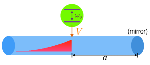
Figure 1: A qubit coupled to a waveguide scatters a single-photon wavepacket injected from the left. The qubit may start in an arbitrary state. The semi-infinite waveguide sketched here is terminated by an effective mirror, thus introducing a delay time.

Waveguide quantum electrodynamics (QED) is an emerging area of quantum optics that investigates coherent coupling between one or more emitters (qubits) and a one-dimensional (1D) photonic waveguide Lodahl et al. (2015); Noh and Angelakis (2017); Liao et al. (2016a); Roy et al. (2017); Gu et al. (2017). Novel correlations among injected near-resonant photons result from the nonlinearity of the qubits, and intriguing interference effects occur because of the 1D confinement of the light. The field has focused on qubits in a local region for which these correlation and interference effects can be used for local quantum information purposes such as single-photon routing Hoi et al. (2011), rectification of photonic signals Dai et al. (2015); Fratini and Ghobadi (2016); Mascarenhas et al. (2016); Fang and Baranger (2017), and quantum gates Koshino et al. (2010); Ciccarello et al. (2012); Zheng et al. (2013). This regime of waveguide QED involves neglecting delay times: the time taken by photons to travel between qubits is far shorter than all other characteristic times. However, an important goal for photonic waveguides is to carry out long-distance quantum information tasks such as quantum state transfer between remote quantum memories Cirac et al. (1997); Kimble (2008). As these necessarily involve distant qubits, delay times cannot be neglected, leading to different kinds of photon correlation and interference effects through the non-Markovian (NM) nature of the system. Here, we study a model waveguide-QED system with large delay time. We apply recent developments in the theory of open quantum systems (OQS) in order to quantitatively assess the qubit’s degree of non-Markovianity.

A large variety of waveguide-QED setups have been experimentally demonstrated in recent years Roy et al. (2017); Gu et al. (2017); Laucht et al. (2012); Goban et al. (2014). Because of high photon group velocities and small systems, these experiments are mostly described by a Markovian approach in which delay times are neglected. In contrast, recent experiments have started entering the regime of non-negligible delay times Roch et al. (2014); Gustafsson et al. (2014); Sundaresan et al. (2015); Chantasri et al. (2016); Liu and Houck (2016), an area that is expected to grow rapidly due to interest in extended systems and long-distance quantum information. Accounting for photon delay times is, however, a challenging theoretical task: only recently have the dynamical effects of long delay times started being investigated Tufarelli et al. (2013); Gonzalez-Ballestero et al. (2013); Zheng and Baranger (2013); Tufarelli et al. (2014); Redchenko and Yudson (2014); Laakso and Pletyukhov (2014); Fang and Baranger (2015); Grimsmo (2015); Shi et al. (2015); Ramos et al. (2016); Guimond et al. (2017). A major consequence of delay times is that NM effects are introduced that affect the physics profoundly, as predicted for e.g. qubit-qubit entanglement in emission Gonzalez-Ballestero et al. (2013); Ramos et al. (2016) and second-order correlation functions in photon scattering Zheng and Baranger (2013); Laakso and Pletyukhov (2014); Fang and Baranger (2015); Shi et al. (2015).

Clarifying the importance of NM effects and the mechanisms behind their onset is thus pivotal in waveguide QED. At the same time, the theory of OQS Breuer and Petruccione (2002); Ángel Rivas and Huelga (2012) is currently making major advances, yielding a more accurate understanding of NM effects Breuer (2012); Rivas et al. (2014); Breuer et al. (2016); de Vega and Alonso (2017). Through an approach often inspired by quantum information concepts Nielsen and Chuang (2000), a number of physical properties such as information back-flow Breuer et al. (2009) and divisibility Rivas et al. (2010) have been spotlighted as distinctive manifestations of quantum NM behavior and then used to formulate corresponding quantum non-Markovianity measures. These tools have been effectively applied to dynamics in various scenarios Rivas et al. (2014); Breuer et al. (2016), including in waveguide QED with regard to emission processes emi ; Ramos et al. (2016); Tufarelli et al. (2014) such as a single atom emitting into a semi-infinite waveguide Tufarelli et al. (2014).

Motivated by the need to quantify NM effects in photon scattering from qubits, we present a case study of a qubit undergoing single-photon scattering in an infinite or semi-infinite waveguide (see Fig. 1), the latter of which is the basis of the proposed controlled-Z Ciccarello et al. (2012) and controlled-Not Zheng et al. (2013) gates. We aim at answering two main questions: What are the essential features of the qubit open dynamics during scattering? Is such dynamics NM? The key task is to find the dynamical map (DM) of the qubit in the scattering process, which fully describes the open dynamics and is needed in order to apply OQS tools Breuer et al. (2016). A distinctive feature of our open dynamics is that the bath (the waveguide field) is initially in a well-defined single-photon state Mirza and Schotland (2016a); Valente et al. (2016). Toward this task, we tackle in full the time evolution of multiple excitations (in contrast to those limited to the one-excitation sector Chen et al. (2011); Liao et al. (2015, 2016b); Mirza and Schotland (2016a); Xiong et al. (2017)), a problem that has become important recently Longo et al. (2010, 2011); Peropadre et al. (2013); Sanchez-Burillo et al. (2015); Grimsmo (2015); Shi et al. (2015); Kocabaş (2016); Ekin Kocabaş (2016); Mirza and Schotland (2016b); Guo et al. (2017); Whalen et al. (2017); Guimond et al. (2017).

Intuitively, one may expect that the dynamics is fully Markovian in the infinite-waveguide case and NM in the semi-infinite case due to the atom-mirror delay time. We show that this expectation is inaccurate in general, mostly because it does not account for a fundamental source of NM behavior namely the wavepacket bandwidth. This NM mechanism is present in an infinite waveguide, while in a semi-infinite waveguide it augments the natural NM behavior coming from the photon delay time. Recently, NM effects in infinite-waveguide scattering were addressed in Ref. Valente et al. (2016). There, however, the qubit is always initially in the ground state, while a fair application of non-Markovianity measures should be based on the entire DM thus requiring consideration of an arbitrary initial state of the qubit.

The paper is organized as follows. We first define the system under consideration in Sec. II. Next, in Sec. III, we find the general form of the the qubit’s DM in a single-photon scattering process and discuss its main features. In Sec. IV, we present the time-dependent master equation (ME), which is fulfilled exactly by the qubit state at any time. In Sec. V, we discuss the explicit computation of the dynamical map in the infinite- and semi-infinite-waveguide case (most of the details regarding the former are given in the Appendix). Since this task requires the time evolution of the scattering process, we in particular find a closed delay partial differential equation that holds in the two-excitation sector of the Hilbert space for a semi-infinite waveguide. In Sec. VI, we assess the non-Markovian nature of the scattering DM by making use of non-Markovianity measures. In this way, we identify two fundamental sources of NM behavior: the finiteness of the wavepacket width and the time-delayed feedback due to the mirror. We finally draw our conclusions in Sec. VII. Some technical details are given in the Appendices.

II System

Consider a qubit with ground (excited) state $|g\rangle$ ($|e\rangle$) and frequency $\omega_{0}$, which is coupled at $x=x_{0}$ to a photonic waveguide (along the $x$-axis) with linear dispersion. We model the system via the standard Shen and Fan (2007a, 2009); Fang and Baranger (2015) real-space Hamiltonian under the rotating-wave approximation (we set $\hbar=c=1$ throughout)

$$\hat{H} =-i\int\limits_{-\infty}^{\xi}\!{\rm d}x\!\left[\hat{a}_{\text{R}}^{\dagger}(x)\partial_{x}\hat{a}_{\text{R}}(x)-\hat{a}_{\text{L}}^{\dagger}(x)\partial_{x}\hat{a}_{\text{L}}(x)\right]+\omega_{0}\hat{\sigma}_{+}\hat{\sigma}_{-}$$

$$\quad+V\int\limits_{-\infty}^{\xi}\!{\rm d}x\,\delta(x-x_{0})\left[\left(\hat{a}^{\dagger}_{\text{R}}(x)+\hat{a}^{\dagger}_{\text{L}}(x)\right)\hat{\sigma}_{-}+{\rm h.c.}\right],$$ (1)

where the bosonic operator $\hat{a}_{\text{R}}(x)$ [$\hat{a}_{\text{L}}(x)$] annihilates a right-going (left-going) photon at $x$, $\hat{\sigma}_{-}=\hat{\sigma}_{+}^{\dagger}=|g\rangle\langle e|$, and $V$ is the qubit-field coupling strength such that the qubit decay rate into the waveguide is $\Gamma=2V^{2}$. For an infinite waveguide, the upper integration limit is $\xi=+\infty$ and $x_{0}=0$, while for a semi-infinite waveguide $\xi=0^{+}$ and $x_{0}=-a$ (see Fig. 1).

III Dynamical map

By definition the qubit’s DM, $\Phi_{t}$, is the superoperator that when applied on any qubit state at $t=0$, $\rho_{0}$, returns its state at time $t>0$ Breuer and Petruccione (2002); Ángel Rivas and Huelga (2012),

$$\rho(t)=\Phi_{t}[\rho_{0}].$$ (2)

The DM fully specifies the open dynamics of the qubit coupled to the waveguide field, with the latter serving as the reservoir.

We now find the DM for a single-photon wavepacket. Let $\hat{U}_{t}=e^{-i\hat{H}t}$ be the unitary evolution operator of the joint qubit-field system. The initial state for single-photon scattering is $\sigma_{0}=\rho_{0}\,|\varphi\rangle\langle\varphi|$ (tensor product symbols are omitted), where $\rho_{0}=\rho_{gg}|g\rangle\langle g|+\rho_{ee}|e\rangle\langle e|+\left(\rho_{ge}|g\rangle\langle e|+{\rm h.c.}\right)$ and $|\varphi\rangle=\int\!{\rm d}x\,\varphi(x)\,\hat{a}_{\rm R}^{\dagger}(x)|{0}\rangle$ is the incoming single-photon (normalized) wavepacket ($|{0}\rangle$ is the waveguide vacuum state). At time $t$, the atom-field state is $\sigma(t)=\hat{U}_{t}\,\sigma_{0}\hat{U}^{\dagger}_{t}=\hat{U}_{t}\rho_{0}\,|\varphi\rangle\langle\varphi|\hat{U}^{\dagger}_{t}$. By plugging $\rho_{0}$ into $\sigma(t)$, we get

$$\sigma(t)=\rho_{gg}\hat{U}_{t}|g\varphi\rangle\langle g\varphi|\hat{U}^{\dagger}_{t}+\rho_{ee}\hat{U}_{t}|e\varphi\rangle\langle e\varphi|\hat{U}^{\dagger}_{t}+\left[\rho_{ge}\hat{U}_{t}|g\varphi\rangle\langle e\varphi|\hat{U}^{\dagger}_{t}+{\rm H.c.}\right],$$ (3)

hence for any $\rho_{0}$ the knowledge of the pair of elementary unitary processes $\hat{U}_{t}|g\varphi\rangle$ and $\hat{U}_{t}|e\varphi\rangle$ fully specifies the time evolution of $\sigma(t)$. Due to the conservation of the total number of excitations [see (1)], the joint evolved state in the two processes has the form

$$|\Psi_{1}(t)\rangle =\hat{U}_{t}|g\rangle|\varphi\rangle=|g\rangle\,|\phi_{1}(t)\rangle+e(t)\,|e\rangle|{0}\rangle,$$ (4)

$$|\Psi_{2}(t)\rangle =\hat{U}_{t}|e\rangle|\varphi\rangle=|g\rangle\,|\chi_{2}(t)\rangle+|e\rangle\,|\psi_{1}(t)\rangle,$$ (5)

where $|\Psi_{n}(t)\rangle$ is the joint wavefunction at time $t$ for $n$ excitations. Here, $|\phi_{1}(t)\rangle$ and $|\psi_{1}(t)\rangle$ are unnormalized single-photon states, and $|\chi_{2}(t)\rangle$ is an unnormalized two-photon state. Note that (4) [(5)] describes the joint dynamics of a single photon scattering off a qubit initially in the ground [excited] state, which takes place entirely in the one-excitation [two-excitation] sector of the Hilbert space. In particular, Eq. (5) is a stimulated emission process Rephaeli and Fan (2012).

The qubit state at time $t$ is the marginal $\rho(t)=\operatorname{Tr}_{\text{field}}\sigma(t)$. This partial trace can be performed by placing Eqs. (4) and (5) into Eq. (3), which yields

$$\rho(t) =\left[\rho_{gg}\|\phi_{1}(t)\|^{2}+\rho_{ee}\|\chi_{2}(t)\|^{2}\right]|g\rangle\langle g|+\left[\rho_{gg}|e(t)|^{2}+\rho_{ee}\|\psi_{1}(t)\|^{2}\right]|e\rangle\langle e|$$

$$\quad+\left[\rho_{ge}\langle\psi_{1}(t)|\phi_{1}(t)\rangle|g\rangle\langle e|+{\rm H.c.}\right],$$ (6)

where we took advantage of orthogonality between one-photon and two-photon states. Since $\{|g\varphi\rangle$, $|e\varphi\rangle\}$ are normalized, so are (4) and (5) due to unitarity of $\hat{U}_{t}$. Thus, $\|\phi_{1}(t)\|^{2}+|e(t)|^{2}=\|\chi_{2}(t)\|^{2}+\|\psi_{1}(t)\|^{2}=1$. By defining three time functions

$$p_{g}(t)\equiv|e(t)|^{2},\quad p_{e}(t)\equiv\|\psi_{1}(t)\|^{2},\quad c(t)\equiv\langle\phi_{1}(t)|\psi_{1}(t)\rangle,$$ (7)

we have $\|\phi_{1}(t)\|^{2}=1-p_{g}(t)$ and $\|\chi_{2}(t)\|^{2}=1-p_{e}(t)$. Therefore, changing to the matrix representation, Eq. (6) takes the form (with $\rho_{ee}=1-\rho_{gg}$)

$$\Phi_{t}[\rho_{0}]=\left(\begin{array}[]{cc}p_{e}(t)-\Delta(t)\rho_{gg}&c(t)\rho_{eg}\\ c^{*}(t)\rho_{eg}^{*}&1-p_{e}(t)+\Delta(t)\rho_{gg}\end{array}\right),$$ (8)

where we defined

$$\Delta(t)\equiv p_{e}(t)-p_{g}(t).$$ (9)

Note that both $p_{g}(t)$ and $p_{e}(t)$ are the qubit excited-state populations but in the two different processes (4) and (5), respectively.

We refer to the qubit DM (8) as the “scattering DM.” Since the atom-field initial state $\sigma_{0}$ is a product state and $\hat{U}_{t}$ is unitary, the map $\Phi_{t}$ is necessarily completely positive (CP) and trace preserving Nielsen and Chuang (2000). In contrast to pure emission processes at zero temperature Breuer and Petruccione (2002), here both the one- and two-excitation sectors are involved. We stress that the DM is fully independent of the qubit’s initial state $\rho_{0}$, being dependent solely on the Hamiltonian (1) and the field initial state $|\varphi\rangle$. This dependance occurs through the functions of time $p_{g/e}(t)$ and $c(t)$ in (8), where $p_{g/e}(t)$ determine the qubit populations while $c(t)$ governs the coherence.

The DM’s form is best understood in the Bloch-sphere picture Nielsen and Chuang (2000) in which a qubit state $\rho$ is represented by the Bloch vector ${\bf r}=(2\operatorname{Re}\rho_{ge},2\operatorname{Im}\rho_{ge},\rho_{gg}-\rho_{ee})$ with $\|{\bf r}\|\leq 1$. In this picture, the map $\Phi_{t}$ is defined by the vector identity

$${\bf r}(t)={\bf M}_{t}{\bf r}_{0}+{\bf v}(t),$$ (10)

where ${\bf v}(t)=\left(0,0,1-p_{e}(t)-p_{g}(t)\right)^{\rm T}$ and ${\bf M}_{t}$ is the $3\times 3$ matrix

$${\bf M}_{t}=\!\left(\begin{array}[]{cc}|c(t)|{\bf R}_{\theta(t)}&{\bf 0}^{\rm T}\\ {\bf 0}&\Delta(t)\end{array}\right).$$ (11)

Here, ${\bf 0}=(0,0)$ while ${\bf R}_{\theta(t)}$ is a standard $2\times 2$ rotation matrix of angle $\theta(t)=\arg[c(t)]$. Thus, apart from the rigid displacement ${\bf v}(t)$ and rotation around the $Z$-axis, the scattering process shrinks the magnitude of the $XY$- and $Z$-components of ${\bf r}(t)$ by the factors $\left|c(t)\right|^{2}$ and $\left|\Delta(t)\right|$, respectively. Since these two factors are generally unequal, the DM transforms the Bloch sphere into an ellipsoid. Such a lack of spherical symmetry does not occur in emission processes Lorenzo et al. (2013), thus providing a hallmark of scattering open dynamics.

In addition, a careful look at Eqs. (10) and (11) shows that the Bloch vector undergoes a reflection across the $XY$-plane whenever $\Delta(t)<0$. This is a further distinctive trait of scattering dynamics, not occurring in emission processes Lorenzo et al. (2013), which is shown below to be relevant to the onset of NM behavior.

IV Non-Markovian Master Equation

The most paradigmatic Markovian dynamics is the one described by the celebrated Lindblad ME Breuer and Petruccione (2002),

$$\dot{\rho}=-i[\hat{\cal H},\rho]+\sum_{\nu}\gamma_{\nu}{\cal L}_{\nu}[\rho],\;\;\textrm{with}\;\;{\cal L}_{\nu}[\rho]=\hat{L}_{\nu}\rho\hat{L}_{\nu}^{\dagger}-(\hat{L}_{\nu}^{\dagger}\hat{L}_{\nu}\rho+\rho\hat{L}_{\nu}^{\dagger}\hat{L}_{\nu})/2,$$ (12)

where $\hat{\cal H}$ is self-adjoint, and all the rates $\gamma_{\nu}$’s are positive constants. In our case, the DM (8) is not described by a Lindblad ME; instead, we show that it is described by a time-dependent ME bra :

$$\dot{\rho}=-i[\hat{\mathcal{H}}(t),\rho]+\gamma_{+}(t)\mathcal{L}_{+}[\rho]+\gamma_{-}(t)\mathcal{L}_{-}[\rho]+\gamma_{z}(t)\mathcal{L}_{z}[\rho]$$ (13)

where $\hat{\mathcal{H}}(t)$ is a time-dependent Hamiltonian, and the jump operators $\hat{L}_{\nu}=\hat{\sigma}_{\nu}$ describe three non-unitary channels with the time-dependent rates $\gamma_{+}(t)$ for absorption, $\gamma_{-}(t)$ for emission, and $\gamma_{z}(t)$ for pure dephasing [explicit forms are given below in Eqs. (16)]. We note that the dephasing term, which reflects the lack of spherical symmetry of the evolved Bloch sphere discussed above, does not occur in spontaneous emission.

The general form for a time-dependent ME is

$$\dot{\rho}=\mathcal{L}_{t}[\rho],$$ (14)

where $\mathcal{L}_{t}$ is a time-dependent linear (and traceless) map, which is fulfilled by $\rho(t)$ as given by Eq. (8). The standard recipe for carrying this out starting from the DM is to first take the derivative of Eq. (2), which yields $\dot{\rho}=\dot{\Phi}_{t}[\rho_{0}]$. Introducing next the inverse of map $\Phi_{t}$, $\Phi_{t}^{-1}$, we can replace $\rho_{0}=\Phi_{t}^{-1}[\rho(t)]$. Hence,

$$\mathcal{L}_{t}=\dot{\Phi}_{t}[\Phi_{t}]^{-1}.$$ (15)

The task now reduces to explicitly calculating $\mathcal{L}_{t}$ and expressing it in a Lindblad form so as to end up with Eq. (13).

This task is efficiently accomplished in the generalized 4-dimensional Bloch space. Recall that the set of four Hermitian operators $\{\hat{G}_{i}\}=\{\openone/\sqrt{2},\hat{\sigma}_{x}/\sqrt{2},\hat{\sigma}_{y}/\sqrt{2},\hat{\sigma}_{z}/\sqrt{2}\}$ — where $i=0,1,2,3$, respectively — is a basis in the qubit operators’s space and fulfills $\operatorname{Tr}\{\hat{G}_{i}\hat{G}_{j}\}=\delta_{ij}$. We express both Eqs. (13) and (15) in this basis and equate them; some details are presented in Appendix A. The resulting expressions for the time-dependent Hamitonian as well as the three time-dependent rates in ME (13) are given by

$$\hat{\mathcal{H}}(t) =-\operatorname{Im}\left[\frac{\dot{c}(t)}{c(t)}\right]\hat{\sigma}_{+}\hat{\sigma}_{-}$$ (16a)

$$\gamma_{+}(t) =\frac{p_{e}(t)\dot{p}_{g}(t)-p_{g}(t)\dot{p}_{e}(t)}{p_{e}(t)-p_{g}(t)},$$ (16b)

$$\gamma_{-}(t) =-\frac{{\dot{p}_{e}(t)-\dot{p}_{g}(t)}}{p_{e}(t)-p_{g}(t)}-\gamma_{+}(t),$$ (16c)

$$\gamma_{z}(t) =-\frac{\gamma_{+}(t)+\gamma_{-}(t)}{4}-\operatorname{Re}\frac{\dot{c}(t)}{2c(t)}.$$ (16d)

It can be checked that when $\hat{\mathcal{H}}(t)$ and these rates are placed in it, ME (13) is exactly fulfilled by Eq. (8) at all times $t$.

Before concluding this section, we note that an exact, differential system (DS) governing the same open dynamics that applies in the case of an infinite waveguide was worked out in Ref. Gheri et al. (1999) and more recently further investigated and generalized in Refs. Baragiola et al. (2012); Gough et al. (2012). For the present case of a single-photon wavepacket and a qubit, this DS has overall three unknowns: two density matrices, one of which is $\rho(t)$, and a traceless non-Hermitian matrix. In contrast to ME (13) here, the DS has the advantage that its time-dependent coefficients are known functions of the wavepacket functional shape (in the time domain). However, since such a DS is not closed with respect to $\rho(t)$ it is less suitable for analyzing the general properties of the qubit’s dynamical map, which is a major goal of the present work. Finally, while ME (13) holds for a qubit coupled to a generic bosonic bath under the rotating-wave approximation, the DS relies on the further hypothesis of a white-noise bosonic bath (hence, in particular, it does not hold in the semi-infinite-waveguide case).

V Explicit computation of DM

For the initial state of the waveguide, throughout this paper we consider an exponential incoming wavepacket of the form

$$\varphi(x)=i\sqrt{\alpha\Gamma}\exp{\left[(ik+\alpha\Gamma/2)(x-x_{0})\right]}\theta(-x+x_{0}),$$ (17)

where $k$ is an arbitrary central frequency, $\alpha\equiv\delta k/\Gamma$ is the wavepacket bandwidth in units of $\Gamma$, and $\theta(x)$ is the step function. This choice of the wavepacket shape is often made (see e.g. Rephaeli and Fan (2012)) as it has at least three advantages. An exponential shape allows for closed-form solutions in the Laplace domain in some cases. In addition, in a numerical approach, its well-defined wavefront leads to a significant reduction in computational time, which is important in the two-photon sector when there is a long time delay. Finally, such wavepackets can be generated experimentally Houck et al. (2007); Bozyigit et al. (2010); Pierre et al. (2014); Pechal et al. (2014); Peng et al. (2016); Forn-Díaz et al. (2017) by either spontaneous emission of a qubit or tunable, on-demand sources.

Our general approach is to plug the ansatz for $|\Psi_{n}(t)\rangle$, Eqs. (4) and (5), into the Schrödinger equation $i\partial_{t}|\Psi_{n}(t)\rangle=\hat{H}|\Psi_{n}(t)\rangle$ to obtain a system of differential equations for the amplitudes that we solve for the three functions $p_{g}(t)$, $p_{e}(t)$, and $c(t)$ in (7) and hence for the DM (8). For an infinite waveguide, this can be accomplished analytically in both the one- and two-excitation sectors as shown in Appendix B. Here, we focus on the far more involved case of a semi-infinite waveguide.

In this case, it is convenient to “unfold” the waveguide semi-axis at the mirror ($x=0$) by introducing a chiral field defined on the entire real axis by $\hat{a}(x)=\hat{a}_{\text{R}}(x)\theta(-x)-\hat{a}_{\text{L}}(x)\theta(x)$ (the minus sign encodes the $\pi$-phase shift due to reflection from the mirror); see Fig. 2. The Hamiltonian (1) can then be rewritten by expressing $\hat{a}_{\text{R}/{\text{L}}}(x)$ in terms of $\hat{a}(x)$ as

$$\hat{H}=-i\int_{-\infty}^{\infty}\!dx\,\hat{a}^{\dagger}(x)\partial_{x}\hat{a}(x)+\omega_{0}\hat{\sigma}_{+}\hat{\sigma}_{-}-iV\!\int_{-\infty}^{\infty}\!dx\!\left[\delta(x+a)-\delta(x-a)\right]\left[\hat{a}^{\dagger}(x)\hat{\sigma}_{-}-\hat{\sigma}_{+}\hat{a}(x)\right].$$ (18)

Compared to Eq. (1), the form of the free-field term shows that only one propagation direction is allowed (chirality) while the term $\propto V$ shows the bi-local coupling of the field to the qubit at points $x=\pm a$ (these can be seen as the locations of the real qubit and its mirror image, respectively).

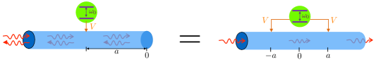
Figure 2: A qubit coupled to a semi-infinite waveguide with qubit-mirror distance $a$ (left) and its equivalent model featuring a qubit coupled to a chiral infinite waveguide at the two points $x=\pm a$ (right).

V.1 Semi-infinite waveguide: one-excitation sector

The wavefunction ansatz in the one-excitation sector is [cf. Eq. (4)]

$$|\Psi_{1}(t)\rangle=\int dx\,\phi(x,t)\hat{a}^{\dagger}(x)|0\rangle+e(t)\hat{\sigma}_{+}|0\rangle,$$ (19)

which once inserted into the Schrödinger equation yields the pair of coupled differential equations

$$i\partial_{t}\phi(x,t) =-i\partial_{x}\phi(x,t)-iVe(t)\left[\delta(x+a)-\delta(x-a)\right],$$ (20a)

$$i\frac{d}{dt}e(t) =\omega_{0}e(t)+iV\left[\phi(-a,t)-\phi(a,t)\right].$$ (20b)

Integration of the photonic part yields the formal solution

$$\phi(x,t)=\phi(x-t,0)-V\left[e(t-x-a)\theta(x+a)\theta(t-x-a)-e(t-x+a)\theta(x-a)\theta(t-x+a)\right],$$ (21)

[cf. Eq. (17) of Ref. Tufarelli et al. (2013)], which once plugged back into the equation for $e(t)$ [Eq. (20b)] yields the delay (ordinary) differential equation (DDE)

$$\frac{de(t)}{dt}=-\left(i\omega_{0}+\frac{\Gamma}{2}\right)e(t)+\frac{\Gamma}{2}e(t-2a)\theta(t-2a)+\sqrt{\frac{\Gamma}{2}}\left[\phi(-a-t,0)-\phi(a-t,0)\right].$$ (22)

Equation (22) is the same as the well-known DDE describing the spontaneous emission process in Refs. Cook and Milonni (1987); Dorner and Zoller (2002); Tufarelli et al. (2013) but with the presence of the extra source term $\propto\sqrt{\Gamma/2}$ due to the incoming photon wavepacket. For the initial conditions $e(0)=0$ and $\phi(x,0)=\varphi(x)$ [cf. Eq. (4)], the solution for $e(t)$ obtained by Laplace transform reads

$$e(t) =\frac{\sqrt{\alpha\Gamma^{2}/2}(e^{-(i\omega_{0}+\Gamma/2)t}-e^{-(ik+\alpha\Gamma/2)t})}{k-\omega_{0}+i\Gamma/2(1-\alpha)}-i\sqrt{\alpha\Gamma}\sum_{n=1}^{\infty}\frac{\left(\frac{\Gamma}{2}\right)^{n-1/2}}{n!}\Bigl{[}(t-2na)^{n}e^{-(i\omega_{0}+\Gamma/2)(t-2na)}$$

$$\quad\quad+\frac{i^{n}(k-\omega_{0}-i\alpha\Gamma/2)}{\left[k-\omega_{0}+i\Gamma/2(1-\alpha)\right]^{n+1}}\gamma(n+1,-ip(t-2na))e^{-(ik+\alpha\Gamma/2)(t-2na)}\Bigr{]}\theta(t-2na)$$ (23)

where $p=k-\omega_{0}+i\Gamma/2(1-\alpha)$ and $\gamma(n,z)$ is the incomplete Gamma function Olver et al. (2010). The corresponding solution for $\phi(x,t)$ follows straightforwardly by using (23) in Eq. (21).

V.2 Semi-infinite waveguide: two-excitation sector

The ansatz for the time-dependent wavefunction [cf. Eq. (5)] reads

$$|\Psi_{2}(t)\rangle=\int dx\,\psi(x,t)\hat{a}^{\dagger}(x)\hat{\sigma}_{+}|0\rangle+\iint dx_{1}dx_{2}\,\chi(x_{1},x_{2},t)\frac{\hat{a}^{\dagger}(x_{1})\hat{a}^{\dagger}(x_{2})}{\sqrt{2}}|0\rangle.$$ (24)

The Schrödinger equation then yields the system of coupled differential equations

$$i\partial_{t}\psi(x,t) =-i\partial_{x}\psi(x,t)+\omega_{0}\psi(x,t)+\frac{iV}{\sqrt{2}}\left[\chi(x,-a,t)+\chi(-a,x,t)-\chi(x,a,t)-\chi(a,x,t)\right],$$ (25a)

$$i\partial_{t}\chi(x_{1},x_{2},t) =-i\left(\partial_{x_{1}}+\partial_{x_{2}}\right)\chi(x_{1},x_{2},t)-\frac{iV}{\sqrt{2}}\left[\psi(x_{1},t)\left(\delta(x_{2}+a)-\delta(x_{2}-a)\right)+x_{2}\leftrightarrow x_{1}\right].$$ (25b)

The formal solution for $\chi(x_{1},x_{2},t)$ is thus

$$\chi(x_{1},x_{2},t) =\chi(x_{1}-t,x_{2}-t,0)-\frac{V}{\sqrt{2}}\biggl{[}\psi(x_{1}-x_{2}-a,t-x_{2}-a)\theta(x_{2}+a)\theta(t-x_{2}-a)$$

$$\quad-\psi(x_{1}-x_{2}+a,t-x_{2}+a)\theta(x_{2}-a)\theta(t-x_{2}+a)+\bigl{(}x_{2}\leftrightarrow x_{1}\bigr{)}\biggr{]},$$ (26)

where note that $\chi$ is symmetrized under the exchange $x_{1}\leftrightarrow x_{2}$. By placing Eq. (26) into Eq. (25a) we find a spatially non-local delay partial differential equation (PDE) for $\psi(x,t)$:

$$\partial_{t}\psi(x,t) =-\partial_{x}\psi(x,t)-\left(i\omega_{0}+\frac{\Gamma}{2}\right)\psi(x,t)+\frac{\Gamma}{2}\psi(x-2a,t-2a)\theta(t-2a)$$ (27)

$$\quad-\frac{\Gamma}{2}\biggl{\{}\bigl{[}\psi(-x-2a,t-x-a)-\psi(-x,t-x-a)\bigr{]}\theta(x+a)\theta(t-x-a)$$

$$\quad\quad+\bigl{[}\psi(2a-x,t-x+a)-\psi(-x,t-x+a)\bigr{]}\theta(x-a)\theta(t-x+a)\biggr{\}}$$

$$\quad+\sqrt{\frac{\Gamma}{4}}\bigl{[}\chi(x-t,-a-t,0)+\chi(-a-t,x-t,0)-\chi(x-t,a-t,0)-\chi(a-t,x-t,0)\bigr{]}.$$

Equation (27) is the two-excitation-sector counterpart of the DDE (22). Mathematically, such a spatially non-local delay PDE is far more involved than the DDE (22) or conventional delay PDEs Zubik-Kowal (2008) that are local in space. A spacetime diagram is shown in Fig. 3.

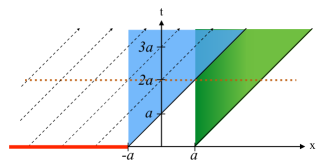
Figure 3: Spacetime diagram for Eq. (27). The dashed lines represent the propagation direction of the initial condition (thick red line). The brown dotted line shows the time after which the delay term appears. The blue and green regions are the light cones of the qubit and its mirror image, respectively.

In our case [cf. Eq. (5)], the initial conditions are $\psi(x,0)=\varphi(x)$ and $\chi(x_{1},x_{2},0)=0$. Due to the latter condition, the terms on the last line of Eq. (27) are identically zero. Hence, overall, the differential equation features four source terms that are non-local in $x$ and $t$ and are non-zero for $x>-a$. In the region $x\leq-a$, the equation takes the simple form

$$\partial_{t}\psi(x,t)=-\partial_{x}\psi(x,t)-\left(i\omega_{0}+\frac{\Gamma}{2}\right)\psi(x,t)+\frac{\Gamma}{2}\psi(x-2a,t-2a)\theta(t-2a).$$ (28)

By taking the Fourier (Laplace) transform with respect to variable $x$ ($t$), this equation is turned into an algebraic equation whose solution is given by

$$\bar{\psi}(q,s) =\frac{\tilde{\varphi}(q)}{s+iq+(i\omega_{0}+\frac{\Gamma}{2})-\frac{\Gamma}{2}e^{-2a(s+iq)}}$$

$$=\frac{\tilde{\varphi}(q)}{s+i(q+\omega_{0})+\frac{\Gamma}{2}}\sum_{n=0}^{\infty}\left[\frac{\frac{\Gamma}{2}e^{-2a(s+iq)}}{s+i(q+\omega_{0})+\frac{\Gamma}{2}}\right]^{n},$$ (29)

where $\tilde{\varphi}(q)={\sqrt{\frac{\alpha\Gamma}{2\pi}}e^{iqa}}/({k-q-i\frac{\alpha\Gamma}{2}})$ is the Fourier transform of $\varphi(x)$. Performing the inverse Fourier transform with respect to $q$ then yields

$$\tilde{\psi}(x,s) =\frac{\sqrt{\alpha\Gamma}}{2\pi}\int dq\,\frac{e^{iq[x-(2n-1)a]}\sum\limits_{n=0}^{\infty}\left[\frac{\frac{\Gamma}{2}e^{-2as}}{s+i(q+\omega_{0})+\frac{\Gamma}{2}}\right]^{n}}{(k-q-i\frac{\alpha\Gamma}{2})\left[s+i(q+\omega_{0})+\frac{\Gamma}{2}\right]}$$

$$=\frac{i\sqrt{\alpha\Gamma}e^{(ik+\alpha\Gamma/2)(x+a)}}{s+i(k+\omega_{0})+\frac{\Gamma}{2}(1+\alpha)}\sum_{n=0}^{\infty}\left[\frac{\frac{\Gamma}{2}e^{-2a(s+ik+\alpha\Gamma/2)}}{s+i(k+\omega_{0})+\frac{\Gamma}{2}(1+\alpha)}\right]^{n},$$ (30)

where we used that, since $x<-a$, only the pole $q=k-i\alpha\Gamma/2$ contributes to the integral. Upon inverse Laplace transform with respect to $s$ term by term, we finally find

$$\psi(x,t)=i\sqrt{\alpha\Gamma}e^{i(k-i\frac{\alpha\Gamma}{2})(x-t+a)}\left\{e^{-(i\omega_{0}+\frac{\Gamma}{2})t}\sum_{n=0}^{\infty}\frac{1}{n!}\left[\frac{\Gamma}{2}e^{(i\omega_{0}+\frac{\Gamma}{2})2a}(t-2na)\right]^{n}\theta(t-2na)\right\}$$ (31)

for $x<-a$. This solution can be expressed compactly as $\psi(x,t)=\varphi(x-t)e_{\rm sm}(t)$, where $e_{\rm sm}(t)$ is the qubit excited-state amplitude in the spontaneous emission process Cook and Milonni (1987); Dorner and Zoller (2002); Tufarelli et al. (2013) namely the solution of Eq. (22) for the initial conditions $e(0)=1$ and $\phi(x,0)=0$. This is physically clear: since the qubit starts in the excited state [cf. Eq. (5)] so long as the photon has not reached its location $x=-a$ the system’s evolution consists of the free propagation of the input single-photon wavepacket and the spontaneous emission as if the field were initially in the vacuum state.

The next natural step would be finding the wavefunction for $-a\leq x\leq a$. However, a look at Eq. (27) shows that such a task is non-trivial. Specifically, two of the source terms, $\psi(-x-2a,t-x-a)$ and $-\psi(-x,t-x-a)$, enter the differential equation which forces one to find the solution “tile by tile” as discussed in the Supplementary Material Sup , a challenging and in the end impractical task. We choose instead to solve the delay PDE numerically by adapting the finite-difference-time-domain (FDTD) method Taflove and Hagness (2005); Schneider (2010); Fang (2017); our approach is described in Ref. Fang (2017). Note that the effectiveness of our code is crucially underpinned by the knowledge of the exact solution for $x<-a$ discussed above Fang (2017).

Finally, once the solutions in both number sectors are found, the three functions $p_{e/g}(t)$ and $c(t)$ can be obtained explicitly as

$$p_{g}(t)=|e(t)|^{2},\quad p_{e}(t)=\int dx\,|\psi(x,t)|^{2},\quad c(t)=\int dx\,\phi^{*}(x,t)\psi(x,t),$$ (32)

where $e(t)$ is given by Eq. (23), $\phi(x,t)$ is given by Eq. (21), and $\psi(x,t)$ is obtained from FDTD.

VI Non-Markovianity

Despite having a Lindblad structure, the time-dependent ME (13) is not in general a Lindblad ME, not even one whose Lindblad generator is time-dependent, because the rates $\{\gamma_{\nu}(t)\}$ are not necessarily all positive at all times Breuer and Petruccione (2002); Ángel Rivas and Huelga (2012); Hall et al. (2014); Breuer et al. (2016). The condition $\gamma_{\nu}(t)\geq 0$ for any $\nu$ and $t$ is indeed violated if $\Delta(t)<0$ at some time $t$ [recall the definition of $\Delta(t)$ in Eq. (9)].

Indeed, since $\Delta(0)=1$, if $\Delta$ becomes negative during the time evolution then there exists an instant at which both $\dot{\Delta}<0$ and $\Delta<0$. Then, since $\gamma_{+}+\gamma_{-}=-\dot{\Delta}/\Delta$ [see Eq. (13) and related text], at least one of the rates $\{\gamma_{\pm}(t)\}$ must be negative at some time. When this happens, the DM is not “CP-divisible”: the dynamics cannot be decomposed into a sequence of infinitesimal CP maps Breuer and Petruccione (2002) each associated with a time $0\leq t^{\prime}\leq t$ and fulfilling (13) with positive rates $\{\gamma_{\nu}(t^{\prime})\}$. Equivalently, it is not governed by a Lindblad ME even locally in time not . Thus, according to the criteria in Refs. Rivas et al. (2010); Hall et al. (2014), the dynamics is NM. Note that the negativity of $\Delta(t)$ is also sufficient to break P-divisibility (a weaker property than CP-divisibility) since it ensures that the sum of at least a pair of time-dependent rates in ME (13) is negative Breuer et al. (2016).

Negativity of $\Delta$ can occur already for an infinite waveguide if the wavepacket width is in an optimal range. Indeed, from the analytic expressions for $p_{e/g}(t)$ in the infinite-waveguide case given in Appendix B.3, we get (time in units of $\Gamma^{-1}$ and $k=\omega_{0}$)

$$\Delta(t)=e^{-(\alpha+1)t}\,\frac{8\alpha e^{\frac{(\alpha+1)t}{2}}+(\alpha-5)(\alpha+1)e^{\alpha t}+4(1-\alpha)}{\alpha^{2}-1}.$$ (33)

Based on elementary analysis, two behaviors are possible (Appendix B.4): for $\alpha>5$, $\Delta(t)\geq 0$ always, while for $0<\alpha\leq 5$, $\Delta(t)$ has a minimum at a negative value at some time. To illustrate this, we plot $\Delta$’s negativity, $N_{\Delta}(t)\equiv-{\rm min}[0,\Delta(t)]$, in Fig. 4. For $0<\alpha\leq 5$, $N_{\Delta}(t)$ is initially zero, then exhibits a maximum at a time of the order of $\Gamma^{-1}$ and eventually decays to zero. For $\alpha\lesssim 10^{-2}$, this maximum is in fact negligible reaching at most $N_{\Delta}\sim\!10^{-6}$ [Fig. 4(b)]. For practical purposes, then, $\Delta(t)$ becomes negative for an optimal range of wavepacket widths $\delta k$ around $\alpha\simeq 1$, i.e., $\delta k\simeq\Gamma$, which excludes small $\alpha$ and hence in particular quasi-plane waves.

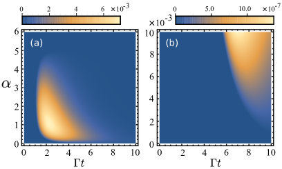
Figure 4: Density plot of the negativity of $\Delta$ as a function of both time $t$ (in units of $\Gamma^{-1}$) and the wavepacket width $\alpha$ for an infinite waveguide. Panel (b) is a small-$\alpha$ zoom of (a). ($k=\omega_{0}=20\Gamma$.)

Rigorously speaking, it should be noted that — as typically happens with time-convolutionless MEs Breuer et al. (2016) — in general there may be singular times at which ME (13) is not defined and correspondingly the DM not invertible. In the present case, these are the times at which $\Delta(t)$ and/or $c(t)$ vanish [cf. Eqs. (9), (16), and (55)]. The above sufficient condition should thus in general be complemented with the additional requirement that $c(t)$ does not simultaneously vanish. This is always the case in Fig. 4, which is easily checked with the help of the analytical expression for $c(t)$ [Eq. (55c)].

Further light on the onset of NM effects can be shed by studying in detail a non-Markovianity measure, which by definition is a function of the entire DM (i.e., at all times) Breuer et al. (2016). Out of the many proposed Breuer et al. (2016), we select the geometric measure (GM) Lorenzo et al. (2013) for its ease of computation and because it facilitates a comparison with the spontaneous emission dynamics in the semi-infinite waveguide where the GM was already used Tufarelli et al. (2014). The GM is defined in terms of the DM’s determinant as Lorenzo et al. (2013)

$$\mathcal{N}=\!\int\limits_{\partial_{t}|\det{\bf M}_{t}|>0}\!\!{\rm d}t\,\frac{{\rm d}}{{\rm d}t}\big{|}\det{\bf M}_{t}\big{|},$$ (34)

where the integral is over all the time intervals in which $|\det{\bf M}_{t}|$ grows in time, and

$$\det{\bf M}_{t}=|c(t)|^{2}\Delta(t)$$ (35)

[cf. Eq. (8)]. Note that $\mathcal{N}$ depends on the modulus of the determinant, which is the volume of the ellipsoid into which the Bloch sphere is transformed by the DM [see Eq. (10)]. Hence, a non-zero $\mathcal{N}$ means this volume increases at some time, in contrast to dynamics described by the Lindblad ME in which such an increase cannot occur Lorenzo et al. (2013). It is known Breuer et al. (2016) that a non-zero GM implies that the dynamics is NM also according to the BLP measure Breuer et al. (2009), which in turn entails NM behavior according to the RHP measure Rivas et al. (2010).

A remarkable property following from Eqs. (34) and (35) is that if there exists a time such that $\Delta(t)<0$ and $c(t)\neq 0$ then ${\big{|}\det{\bf M}_{t}\big{|}}$ must grow at some time. This then brings about that the dynamics is NM according to the GM (34) and hence NM even according to the BLP and RHP measures. We thus in particular retrieve the sufficient condition for breaking P- and CP-divisibility discussed at the beginning of this section since non-zero BLP (RHP) measure ensures violation of P-divisibility (CP-divisibility) Breuer et al. (2016).

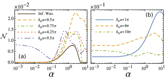
Figure 5: The geometric non-Markovianity measure $\mathcal{N}$ as a function of the dimensionless wavepacket bandwidth $\alpha$ on a linear-log scale. (a) Infinite waveguide (solid line) and semi-infinite waveguide for non-integer values of $k_{0}a/\pi$. (b) Semi-infinite waveguide for integer values of $k_{0}a/\pi$. Note the different vertical axis scale in the two panels. Non-Markovianity is larger for the semi-infinite-waveguide case (especially for integer $k_{0}a/\pi$) because of the time delay in reflecting from the (distant) mirror. ($k=k_{0}=\omega_{0}=20\Gamma$.)

Figure 5(a) shows $\mathcal{N}$ for the infinite-waveguide case for a wavepacket carrier frequency resonant with the qubit (solid line). Similarly to the negativity of $\Delta$, $\mathcal{N}$ takes significant values only around $\alpha\simeq 1$ (i.e., $\delta k\simeq\Gamma$), being negligible in particular for quasi-monochromatic wavepackets. The values of $\alpha$ yielding $\mathcal{N}\neq 0$ are also such that the dynamics is NM according to the BLP measure Breuer et al. (2009) and even the RHP measure Rivas et al. (2010), the latter meaning that rates $\gamma_{\pm,z}(t)$ in the ME (13) break the condition of being positive at all time.

The behavior of $\mathcal{N}$ changes substantially for a semi-infinite waveguide, as shown in Fig. 5 for several values of the qubit-mirror distance $a$. First, non-Markovianity is generally larger, even by an order of magnitude in some cases [note the difference in scale between panels (a) and (b)]. Second, $\mathcal{N}$ can be significant even at $\alpha\simeq 0$ (the plane-wave limit), in which case it matches its value in the corresponding spontaneous-emission process Tufarelli et al. (2014). For our parameters, the maximum non-Markovianity in this limit occurs near $k_{0}a=4\pi$. Third, $\mathcal{N}$ exhibits a more structured behavior as a function of $\alpha$, the shape of $\mathcal{N}(\alpha)$ being dependent on $k_{0}a$ (recall $k_{0}=\omega_{0}$).

The feedback due to the mirror, evident in Eqs. (22) and (27), generally introduces memory effects in the qubit dynamics that are expected to cause NM behavior. These add to the finite-wavepacket effect already occurring with no mirror, leading generally to enhanced non-Markovianity—note that the semi-infinite-waveguide curves in Fig. 5 typically lie above the mirrorless one. The non-Markovianity can be especially large when either $2k_{0}a$, the phase corresponding to a qubit-mirror round trip, is an integer multiple of 2$\pi$ and/or the corresponding photon delay time $\uptau=2a$ is large compared to the atom decay time $\Gamma^{-1}$. In the former case, enhanced NM behavior occurs because a standing wave can form between the mirror and the qubit under these conditions; indeed, it has been shown that a bound state in the continuum exists in this system Tufarelli et al. (2013). In the latter case, the fact that the qubit decays completely before the photon returns causes a periodic re-excitation of the qubit—a kind of revival.

We found numerically that the scattering DM (8) reduces to that for spontaneous emission Tufarelli et al. (2014) in the limits of very large and very small $\alpha$, thus in particular explaining the behavior of $\mathcal{N}$ at $\alpha\simeq 0$. In the infinite-waveguide case, this property can be shown analytically (see Appendix B.3). Physically, these limits can be viewed as follows. When $\alpha\simeq 0$, the wavepacket is so spread out spatially that the photon density at the qubit is negligible: the qubit effectively sees a vacuum, hence behaving as in spontaneous emission. This clarifies why NM effects cannot occur without the mirror for a quasi-plane-wave (the emission DM in an infinite waveguide is clearly Markovian). When $\alpha\gg 1$ in contrast, the photon is very localized at the qubit position. The energy-time uncertainly principle then implies that the photon passes too fast for the qubit to sense, hence the qubit again behaves as if the field were in the vacuum state.

Since non-Markovianity measures are generally not equivalent Breuer et al. (2016) it is natural to wonder whether the outcomes of our analysis in Fig. 5 for the GM hold qualitatively if a different measure is used, for instance the widely adopted BLP measure Breuer et al. (2009). While a comprehensive comparative study of different measures is beyond the scope of the present paper, we computed the BLP measure ${\cal N}_{\rm BLP}$ for some representative values of the parameters. For an infinite waveguide, the behavior of ${\cal N}_{\rm BLP}$ as a function of $\alpha$ is analogous to that of the GM [see Fig. 5(a)]. In the semi-infinite-waveguide case, ${\cal N}_{\rm BLP}$ overall behaves similarly to the GM but exhibits a less structured shape: for instance, the inflection point for $k_{0}a=0.5\pi$ in Fig. 5(a) is absent.

VII Conclusions

We studied the open dynamics of a qubit coupled to a 1D waveguide during single-photon scattering, presenting results for its DM, the corresponding time-dependent ME, and rigorous non-Markovianity measures developed in OQS theory. The qubit dynamics was shown to have distinctive features that, in particular, do not occur in emission processes. To compute the DM for a semi-infinite waveguide, we solved the scattering time evolution by deriving a spatially non-local delay PDE for the one-photon wavefunction when the qubit is excited. For an infinite waveguide, NM behavior occurs when the photon-wavepacket bandwidth $\delta k$ is of order the qubit decay rate $\Gamma$. For a semi-infinite waveguide (mirror), time delay effects are an additional source of non-Markovianity, resulting in generally stronger NM effects.

The system we studied here, a semi-infinite waveguide plus a qubit, is the simplest waveguide QED system with a time delay. Yet the nature and effects of the time delay should be completely generic as there is no fine tuning in our system. We thus expect these main conclusions to also hold in, for instance, the case of two distant qubits coupled to a waveguide which is relevant for long-distance quantum information.

It is interesting to note [see Eq. (35)] that $\Delta(t)$ has the same sign as $\det{\bf M}_{t}$, hence times can exist at which $\det{\bf M}_{t}<0$. Among qubit CP maps, those with negative determinant are the only ones that break the property of being “infinitesimally divisible” Wolf and Cirac (2008). This class does not include spontaneous-emission DMs—in particular vacuum Rabi oscillations—where the determinant is always non-negative Lorenzo et al. (2013). In sharp contrast, the scattering DMs studied here do belong to this class.

Finally, we note that some results here rely solely on the DM structure (8) that in turn stems solely from having an initial Fock state for the field and the rotating wave approximation. Further investigation of this class of open dynamics is under way wip .

Appendix A Derivation of the time-dependent ME

In this Appendix, we present some details of the derivation of the time-dependent ME, Eq. (13). In particular, we express both Eqs. (13) and (15) using as a basis the four Hermitian operators $\{\hat{G}_{i}\}=\{\openone/\sqrt{2},\hat{\sigma}_{x}/\sqrt{2},\hat{\sigma}_{y}/\sqrt{2},\hat{\sigma}_{z}/\sqrt{2}\}$ with $i=0,1,2,3$, respectively; recall that $\operatorname{Tr}\{\hat{G}_{i}\hat{G}_{j}\}=\delta_{ij}$. An operator $\rho$ (and so in particular a density operator) can be decomposed as $\rho=\sum_{i=0}^{3}r_{i}\hat{G}_{i}$ with $r_{i}=\operatorname{Tr}\{\hat{G}_{i}\rho\}$, hence the 4-dimensional real vector $\bf r$ is a representation of the density operator $\rho$. A map is analogously represented by a $4{\times}4$ transformation matrix.

For ${\cal L}_{t}$ we start by noting that the dynamical map can be expressed as

$$\Phi_{t}[\rho] =\sum_{j}\Phi_{t}(r_{j}\hat{G}_{j})=\sum_{j}r_{j}\Phi_{t}\hat{G}_{j}=\sum_{j}r_{j}\sum_{k}\operatorname{Tr}\left\{\hat{G}_{k}\Phi_{t}\hat{G}_{j}\right\}\hat{G}_{k}$$

$$=\sum_{k}\left(\sum_{j}\operatorname{Tr}\{\hat{G}_{k}\Phi_{t}\hat{G}_{j}\}r_{j}\right)\hat{G}_{k}=\sum_{k}\left(\mathbf{F}\,\mathbf{r}\right)_{k}\hat{G}_{k},$$ (36)

where we used the linearity of $\Phi_{t}$ and defined the entries of the $4{\times}4$ matrix $\mathbf{F}$ as

$$F_{kj}=\operatorname{Tr}\left\{\hat{G}_{k}\Phi_{t}\hat{G}_{j}\right\}.$$ (37)

The matrix $\mathbf{F}$ thus represents the map $\Phi_{t}$ (we drop the time dependance for simplicity). The composition of two maps is correspondingly turned into the matrix product of the associated matrices [each defined analogously to Eq. (37)]. Hence, if $\mathbf{L}$ is the 4$\times 4$ matrix associated with map $\mathcal{L}_{t}$ [see Eq. (15)], it is given by

$$\mathbf{L}=\dot{\mathbf{F}}\,\mathbf{F}^{-1}.$$ (38)

We are thus led to compute the (time-dependent) matrix $\bf F$, calculate its derivative $\dot{\bf F}$ and inverse $\bf F^{-1}$, and finally take the matrix product (38). To calculate $\bf F$ we use Eqs. (8) and (37), where the matrix elements $\rho_{ij}$ entering Eq. (8) are now the matrix entries of operators $\{\hat{G}_{j}\}$ (for instance, $\hat{G}_{1}=\hat{\sigma}_{x}/\sqrt{2}$ has entries $(G_{1})_{ee}=(G_{1})_{gg}=0$ and $(G_{1})_{eg}=(G_{1})_{ge}=1/\sqrt{2}$). By proceeding in this way, matrix $\bf F$ reads

$${\bf F}=\left(\begin{array}[]{cccc}1&0&0&0\\ 0&\operatorname{Re}[c(t)]&\operatorname{Im}[c(t)]&0\\ 0&-\operatorname{Im}[c(t)]&\operatorname{Re}[c(t)]&0\\ p_{e}(t)+p_{g}(t)-1&0&0&p_{e}(t)-p_{g}(t)\end{array}\right).$$ (39)

Using this and Eq. (38), we find that matrix ${\bf L}$ is

$${\bf L}=\left(\begin{array}[]{cccc}0&0&0&0\\ 0&\operatorname{Re}\left[\frac{\dot{c}(t)}{c(t)}\right]&\operatorname{Im}\left[\frac{\dot{c}(t)}{c(t)}\right]&0\\ 0&-\operatorname{Im}\left[\frac{\dot{c}(t)}{c(t)}\right]&\operatorname{Re}\left[\frac{\dot{c}(t)}{c(t)}\right]&0\\ \frac{\dot{p}_{e}(t)+\dot{p}_{e}(t)}{p_{g}(t)+p_{e}(t)-1}+2\,\frac{\,\left[1-p_{g}(t)\right]\dot{p}_{e}(t)+p_{e}(t)\dot{p}_{g}(t)}{1-p_{g}(t)-p_{e}(t)}&0&0&\frac{\dot{p}_{g}(t)+\dot{p}_{e}(t)}{p_{g}(t)+p_{e}(t)-1}\end{array}\right).$$ (40)

This shows that Eq. (14) holds with the generator $\mathcal{L}_{t}$ whose 4$\times$4-matrix representation is given by Eq. (40).

The remaining step is to show that the generator can indeed be expressed as the right-hand side of (13). To this aim, we consider Eq. (13) without specifying $\hat{H}(t)$, $\gamma_{\pm}(t)$ and $\gamma_{z}(t)$, work out its 4$\times$4-matrix representation, impose that it yields $\dot{\bf r}={\bf L}{\bf r}$ with ${\bf L}$ given by Eq. (40) and solve for $\hat{H}(t)$, $\gamma_{\pm}(t)$ and $\gamma_{z}(t)$. Thus let us define

$$\tilde{\mathcal{L}}_{t}[\rho]=\!-i\left[\frac{S(t)}{2}\,\hat{\sigma}_{+}\hat{\sigma}_{-}+\mu(t)\hat{\sigma}_{+}+\mu^{*}(t)\hat{\sigma}_{-},\rho\right]+\!\gamma_{-}(t)\mathcal{L}_{-}[\rho]+\!\gamma_{+}(t)\mathcal{L}_{+}[\rho]+\!\gamma_{z}(t)\mathcal{L}_{z}[\rho]$$ (41)

and call $\tilde{\bf L}$ the associated 4$\times 4$ matrix. To compute $\tilde{\bf L}$, in Eq. (41) we replace $\rho=\sum_{i}r_{i}\hat{G}_{i}$ and calculate $\operatorname{Tr}\{\hat{A}\,\hat{G}_{i}\,\hat{B}\}$ with $\hat{A},\hat{B}=\hat{G}_{0},...,\hat{G}_{3}$, obtaining

$${\bf\tilde{L}}=\left(\begin{array}[]{cccc}0&0&0&0\\ 0&-\frac{\gamma_{+}(t)+\gamma_{-}(t)}{2}-2{\gamma_{z}(t)}&-\frac{S(t)}{2}&-2\,\operatorname{Im}[\mu(t)]\\ 0&\frac{S(t)}{2}&-\frac{\gamma_{+}(t)+\gamma_{-}(t)}{2}-2{\gamma_{z}(t)}&-2\,\operatorname{Re}[\mu(t)]\\ \gamma_{+}(t)-\gamma_{-}(t)&2\,\operatorname{Im}[\mu(t)]&2\,\operatorname{Re}[\mu(t)]&-\left[\gamma_{+}(t)+\gamma_{-}(t)\right]\\ \end{array}\right).$$ (42)

We next require that Eq. (42) equals Eq. (40). Upon comparison of these two equations, we immediately get $\mu(t)=0$, while $S(t)=-2\operatorname{Im}\left[\dot{c}(t)/c(t)\right]$. Moreover, by requiring the entries $L_{22}$, $L_{44}$ and $L_{41}$ of matrix (42) to match the corresponding ones of (40), we find the three rates given in Eq. (16).

Appendix B Calculations for the infinite-waveguide case

Here, we present details of the calculation of the time-dependent wavefunctions in both the one- and two-excitation sectors that are needed for the explicit calculation of the dynamical map Eq. (8) in the infinite-waveguide case. Following the main text, we refer to $\varphi(x)$ as a single-photon exponential wavepacket of the form Eq. (17). Further technical details, including the study of other possible initial conditions, are given in the Supplementary Material Sup .

B.1 One-excitation sector

This is the scattering process corresponding to Eq. (4) in the infinite-waveguide case, based on which the ansatz for the time-dependent wavefunction reads

$$|\Psi_{1}(t)\rangle=\int dx\left[\phi_{\text{R}}(x,t)\hat{a}_{\text{R}}^{\dagger}(x)+\phi_{\text{L}}(x,t)\hat{a}_{\text{L}}^{\dagger}(x)\right]|0\rangle+e(t)\hat{\sigma}_{+}|0\rangle,$$ (43)

where $\phi_{\text{R/L}}(x,t)$ is the wavefunction of the right-/left-going photon.

Imposing the Schrödinger equation, $i\partial_{t}|\Psi_{1}(t)\rangle=\hat{H}|\Psi_{1}(t)\rangle$, yields the three coupled equations

$$i\partial_{t}\phi_{\text{R}}(x,t) =-i\partial_{x}\phi_{\text{R}}(x,t)+Ve(t)\delta(x),$$ (44a)

$$i\partial_{t}\phi_{\text{L}}(x,t) =i\partial_{x}\phi_{\text{L}}(x,t)+Ve(t)\delta(x),$$ (44b)

$$i\frac{d}{dt}e(t) =\omega_{0}e(t)+V\left[\phi_{\text{R}}(0,t)+\phi_{\text{L}}(0,t)\right].$$ (44c)

The equations for $\phi_{\text{R/L}}(x,t)$ can be formally integrated by Fourier transform, yielding

$$\phi_{\text{R}}(x,t) =\phi_{\text{R}}(x-t,0)-iVe(t-x)\theta(x)\theta(t-x),$$ (45a)

$$\phi_{\text{L}}(x,t) =\phi_{\text{L}}(x+t,0)-iVe(t+x)\theta(-x)\theta(t+x),$$ (45b)

where we set $\theta(0)\equiv 1/2$. The first term on each righthand side describes the free-field behavior, while the second one can be interpreted as a source term originating from qubit emission at an earlier time. Note that causality is preserved as it should be. Eqs. (45) immediately entail $\phi_{\text{R}}(0,t)+\phi_{\text{L}}(0,t)=\phi_{\text{R}}(-t,0)+\phi_{\text{L}}(t,0)-iVe(t)$, which once substituted in Eq. (44c) yields a time-local first-order differential equation for $e(t)$

$$\frac{d}{dt}e(t)=-\left(i\omega_{0}+\frac{\Gamma}{2}\right)e(t)-iV\left[\phi_{\text{R}}(-t,0)+\phi_{\text{L}}(t,0)\right].$$ (46)

Imposing the initial conditions $\phi_{\text{R}}(x,0)=\varphi(x)$, $\phi_{\text{L}}(x,0)=e(0)=0$, we obtain,

$$e(t)=\frac{i\sqrt{\alpha\Gamma^{2}/2}\left(e^{-(ik+\alpha\Gamma/2)t}-e^{-(i\omega_{0}+\Gamma/2)t}\right)}{k-\omega_{0}+i\Gamma(1-\alpha)/2}.$$ (47)

By using Eq. (47) in Eqs. (45), one then obtains the photon wavefunctions $\phi_{\text{R/L}}(x,t)$.

B.2 Two-excitation sector

Based on Eq. (5), the ansatz for the time-dependent wavefunction reads

$$|\Psi_{2}(t)\rangle =\int\!\!dx\left[\psi_{\text{R}}(x,t)\hat{a}_{\text{R}}^{\dagger}(x)+\psi_{\text{L}}(x,t)\hat{a}_{\text{L}}^{\dagger}(x)\right]\hat{\sigma}_{+}|0\rangle+\iint\!\!dx_{1}dx_{2}\Bigl{[}\chi_{\text{RR}}(x_{1},x_{2},t)\frac{\hat{a}_{\text{R}}^{\dagger}(x_{1})\hat{a}_{\text{R}}^{\dagger}(x_{2})}{\sqrt{2}}$$

$$\quad+\chi_{\text{RL}}(x_{1},x_{2},t)\hat{a}_{\text{R}}^{\dagger}(x_{1})\hat{a}_{\text{L}}^{\dagger}(x_{2})+\chi_{\text{LL}}(x_{1},x_{2},t)\frac{\hat{a}_{\text{L}}^{\dagger}(x_{1})\hat{a}_{\text{L}}^{\dagger}(x_{2})}{\sqrt{2}}\Bigr{]}|0\rangle,$$ (48)

where $\psi_{\text{R/L}}(x,t)$ is the probability amplitude to have a right-/left-propagating photon at position $x$ with the qubit in the excited state, while $\chi_{\alpha\beta}(x_{1},x_{2},t)$ is the probability amplitude to have an $\alpha$-propagating photon at position $x_{1}$ and a $\beta$-propagating photon at position $x_{2}$ (with the qubit unexcited). Terms $\propto\chi_{\text{LR}}$ have been incorporated in those $\propto\chi_{\text{RL}}$ by exploiting the symmetrization property $\chi_{\text{LR}}(x_{1},x_{2},t)=\chi_{\text{RL}}(x_{2},x_{1},t)$. The Schrödinger equation then yields five coupled differential equations that read

$$\partial_{t}\psi_{\text{R}}(x,t) =-\partial_{x}\psi_{\text{R}}(x,t)-i\omega_{0}\psi_{\text{R}}(x,t)-iV\left[\frac{\chi_{\text{RR}}(0,x,t)+\chi_{\text{RR}}(x,0,t)}{\sqrt{2}}+\chi_{\text{RL}}(x,0,t)\right],$$ (49a)

$$\partial_{t}\psi_{\text{L}}(x,t) =\partial_{x}\psi_{\text{L}}(x,t)-i\omega_{0}\psi_{\text{L}}(x,t)-iV\left[\frac{\chi_{\text{LL}}(0,x,t)+\chi_{\text{LL}}(x,0,t)}{\sqrt{2}}+\chi_{\text{RL}}(0,x,t)\right],$$ (49b)

$$\partial_{t}\chi_{\text{RR}}(x_{1},x_{2},t) =-\left(\partial_{x_{1}}+\partial_{x_{2}}\right)\chi_{\text{RR}}(x_{1},x_{2},t)-\frac{iV}{\sqrt{2}}\left[\psi_{\text{R}}(x_{1},t)\delta(x_{2})+\psi_{\text{R}}(x_{2},t)\delta(x_{1})\right],$$ (49c)

$$\partial_{t}\chi_{\text{RL}}(x_{1},x_{2},t) =-\left(\partial_{x_{1}}-\partial_{x_{2}}\right)\chi_{\text{RL}}(x_{1},x_{2},t)-iV\left[\psi_{\text{R}}(x_{1},t)\delta(x_{2})+\psi_{\text{L}}(x_{2},t)\delta(x_{1})\right],$$ (49d)

$$\partial_{t}\chi_{\text{LL}}(x_{1},x_{2},t) =\left(\partial_{x_{1}}+\partial_{x_{2}}\right)\chi_{\text{LL}}(x_{1},x_{2},t)-\frac{iV}{\sqrt{2}}\left[\psi_{\text{L}}(x_{1},t)\delta(x_{2})+\psi_{\text{L}}(x_{2},t)\delta(x_{1})\right].$$ (49e)

Note that the equations for $\chi_{\text{RR}}$ and $\chi_{\text{LL}}$ are symmetrized because of the bosonic statistics. Similarly to the previous subsection, we first formally solve for the purely photonic wavefunctions and find

$$\chi_{\text{RR}}(x_{1},x_{2},t) =\chi_{\text{RR}}(x_{1}-t,x_{2}-t,0)-\frac{iV}{\sqrt{2}}\bigl{[}\psi_{\text{R}}(x_{1}-x_{2},t-x_{2})\theta(x_{2})\theta(t-x_{2})$$

$$\quad+\psi_{\text{R}}(x_{2}-x_{1},t-x_{1})\theta(x_{1})\theta(t-x_{1})\bigr{]},$$ (50a)

$$\chi_{\text{RL}}(x_{1},x_{2},t) =\chi_{\text{RL}}(x_{1}-t,x_{2}+t,0)-iV\bigl{[}\psi_{\text{R}}(x_{1}+x_{2},t+x_{2})\theta(-x_{2})\theta(t+x_{2})$$

$$\quad+\psi_{\text{L}}(x_{2}+x_{1},t-x_{1})\theta(x_{1})\theta(t-x_{1})\bigr{]},$$ (50b)

$$\chi_{\text{LL}}(x_{1},x_{2},t) =\chi_{\text{LL}}(x_{1}+t,x_{2}+t,0)-\frac{iV}{\sqrt{2}}\bigl{[}\psi_{\text{L}}(x_{1}-x_{2},t+x_{2})\theta(-x_{2})\theta(t+x_{2})$$

$$\quad+\psi_{\text{L}}(x_{2}-x_{1},t+x_{1})\theta(-x_{1})\theta(t+x_{1})\bigr{]}.$$ (50c)

Next, we plug these solutions back into Eqs. (49a) and (49b), which are those featuring the qubit degree of freedom, under the initial condition that $\chi_{\alpha\beta}(x_{1},x_{2},0)=0$ for any $\alpha,\beta={\rm L},{\rm R}$. The resulting pair of equations read

$$\partial_{t}\psi_{\text{R}}(x,t) =-\partial_{x}\psi_{\text{R}}(x,t)-\left(i\omega_{0}+\frac{\Gamma}{2}\right)\psi_{\text{R}}(x,t)-\frac{\Gamma}{2}\left[\psi_{\text{R}}(-x,t-x)+\psi_{\text{L}}(x,t-x)\right]\theta(x)\theta(t-x),$$ (51a)

$$\partial_{t}\psi_{\text{L}}(x,t) =\partial_{x}\psi_{\text{L}}(x,t)-\left(i\omega_{0}+\frac{\Gamma}{2}\right)\psi_{\text{L}}(x,t)-\frac{\Gamma}{2}\left[\psi_{\text{R}}(x,t+x)+\psi_{\text{L}}(-x,t+x)\right]\theta(-x)\theta(t+x).$$ (51b)

These coupled differential equations are non-local with respect to both $x$ and $t$, the non-locality being due to the rightmost “source terms” that feature the double step functions. Based on the arguments of the step functions, it is natural to partition space-time into the three regions $x\leq 0$ (${\rm R}_{1}$), $0<x\leq t$ (${\rm R}_{2}$), and $x>t$ (${\rm R}_{3}$) in the case of Eq. (51a) and $x\leq-t$ (${\rm L}_{3}$), $-t<x\leq 0$ (${\rm L}_{2}$), and $x>0$ (${\rm L}_{1}$) in the case of Eq. (51b), as shown in Fig. 6. Then, the differential equations (51) can be analytically solved in four steps as follows:

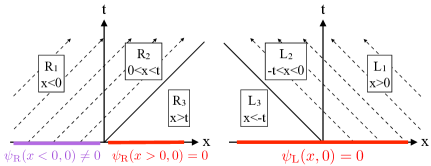
Figure 6: Partitions of space-time in the case of Eqs. (51a) and (51b), left and right panels, respectively.

1. Solve Eq. (51a) for $\psi_{\text{R}}(x,t)$ in region $\text{R}_{1}$ under the initial (i.e., boundary) condition $\psi_{\text{R}}(x,0)=\varphi(x)$. In this region, the source term is identically zero.

2. Solve Eq. (51b) for $\psi_{\text{L}}(x,t)$ in region $\text{L}_{1}$ under the initial (i.e., boundary) condition $\psi_{\text{L}}(x,0)=0$. As the source term is also identically zero in this region, we trivially get $\psi_{\text{L}}(x>0,t)=0$.

3. Solve Eq. (51a) for $\psi_{\text{R}}(x,t)$ in region $\text{R}_{2}$ under the boundary condition $\psi_{\text{R}}(0,t)$ [this being fully specified by the solution found at step (i)]. In this region, the source term is non-zero but is fully specified by the solutions $\psi_{\text{R}}(x<0,t)$ and $\psi_{\text{L}}(x>0,t)$ worked out at the previous steps (i) and (ii), respectively. Note that the initial condition automatically guarantees that the wavefunction is continuous at $x=0$.

4. Solve Eq. (51b) analogously for $\psi_{\text{L}}(x,t)$ in region $\text{L}_{2}$ under the boundary condition $\psi_{\text{L}}(0,t)=0$. In this region, the source term is again fully specified by the solutions $\psi_{\text{R}}(x<0,t)$ and $\psi_{\text{L}}(x>0,t)$ obtained in the previous steps.

Finally, $\psi_{\text{R}}(x,t)$ vanishes identically in region $\text{R}_{3}$ and, likewise, so does $\psi_{\text{L}}(x,t)$ in region $\text{L}_{3}$. This is because causality prevents the wavefunction outside the light cone from being affected by the qubit or input wave. Since initially the wavefunction is zero in this region, it remains so at all times. Hence, the wavefunction is non-zero only in regions R₁, R₂ and L₂.

With the help of Mathematica (see Supplementary Material Sup ), the above procedure straightforwardly yields analytical expressions for the wavefunctions. We checked that, in the steady-state limit $t{\rightarrow}\infty$, the above solution for the wavefunctions in the stimulated-emission problem yields results in full agreement with those obtained via a time-independent approach Rephaeli and Fan (2012). In particular, the two-photon scattering outcome probabilities $P_{\text{RR}}$, $P_{\text{RL}}$ and $P_{\text{LL}}$ of Ref. Rephaeli and Fan (2012) are recovered as

$$P_{\alpha\beta}=\lim_{t\rightarrow\infty}\int_{-\infty}^{\infty}dx_{1}\int_{-\infty}^{\infty}dx_{2}|\chi_{\alpha\beta}(x_{1},x_{2},t)|^{2},$$ (52)

with $\alpha,\beta\in\{\text{R},\text{L}\}$.

We finally mention that, in the case of an incoming two-photon wavepacket (not addressed in the main text), one or more terms $\chi_{\alpha\beta}(x_{1},x_{2},0)$ are non-zero and Eqs. (51) feature additional terms. For instance, in the case of a left-incoming two-photon wavepacket, the additional term $-i\sqrt{\Gamma/4}\bigl{[}\chi_{\text{RR}}(x-t,-t,0)+\chi_{\text{RR}}(-t,x-t,0)\bigr{]}$ must be added to the right-hand side of Eq. (51a). In this case, in the steady-state limit $t\rightarrow\infty$ known results for two-photon scattering (in particular second-order correlation functions) Shen and Fan (2007b); Zheng et al. (2010); Zheng and Baranger (2013); Fang and Baranger (2015) are recovered, which confirms the effectiveness of our real-space time-dependent approach.

B.3 Functions $p_{g}(t)$, $p_{e}(t)$ and $c(t)$

The three functions (7), which fully specify the scattering DM (8), are found from Eqs. (4), (5), (43), (48) to be $p_{g}(t)=|e(t)|^{2}$,

$$p_{e}(t) =\|\psi_{1}(t)\|^{2}=\int dx\left[|\psi_{\text{R}}(x,t)|^{2}+|\psi_{\text{L}}(x,t)|^{2}\right],$$ (53)

$$c(t) =\langle\phi_{1}(t)|\psi_{1}(t)\rangle=\int dx\left[\phi_{\text{R}}^{*}(x,t)\psi_{\text{R}}(x,t)+\phi_{\text{L}}^{*}(x,t)\psi_{\text{L}}(x,t)\right].$$ (54)

Thus, after using Eqs. (45) and (47), rescaling time in units of $\Gamma^{-1}$, and setting $k=\omega_{0}$, they are explicitly given for the infinite-waveguide case by

$$p_{g}(t) =2\alpha e^{-t}\left[\frac{e^{-\frac{1}{2}(\alpha-1)t}-1}{\alpha-1}\right]^{2},$$ (55a)

$$p_{e}(t) =e^{-(\alpha\!+\!1)t}\frac{-4(\alpha-1)^{2}+\left(\alpha^{3}-3\alpha^{2}+\alpha+5\right)e^{\alpha t}+4(\alpha-3)\alpha e^{\frac{1}{2}(\alpha+1)t}+2\alpha(\alpha+1)e^{t}}{(\alpha-1)^{2}(\alpha+1)},$$ (55b)

$$c(t) =e^{-(\alpha+1+i\omega_{0})t}\frac{(\alpha-1)^{2}e^{\left(\alpha+\frac{1}{2}\right)t}+4\alpha e^{\frac{\alpha t}{2}}-2(\alpha+1)e^{t/2}}{\alpha^{2}-1}.$$ (55c)

From Eqs. (55a) and (55b), the quantity $\Delta(t)$ in the infinite-waveguide case is easily obtained as given in Eq. (33).

In the two limits $\alpha\rightarrow 0$ and $\alpha\rightarrow\infty$ (see main text), we get

$$\lim_{\alpha\to 0}p_{g}(t)=\lim_{\alpha\to\infty}p_{g}(t)=0,\quad\lim_{\alpha\to 0}p_{e}(t)=\lim_{\alpha\to\infty}p_{e}(t)=e^{-\Gamma t},\quad\lim_{\alpha\to 0}c(t)=\lim_{\alpha\to\infty}c(t)=e^{-i\omega_{0}t}e^{-\frac{\Gamma}{2}t}$$

with Eq. (8) thereby reducing to

$$\Phi_{t}[\rho_{0}]=\left(\begin{array}[]{cc}e^{-\Gamma t}\rho_{ee}&e^{-i\omega_{0}t}e^{-\frac{\Gamma}{2}t}\rho_{eg}\\ e^{i\omega_{0}t}e^{-\frac{\Gamma}{2}t}\rho_{eg}^{*}&\rho_{gg}+(1-e^{-\Gamma t})\rho_{ee}\end{array}\right).$$ (56)

This is the DM of spontaneous emission into an infinite waveguide with a flat spectral density Breuer and Petruccione (2002) obeying the time-independent Lindblad ME $\dot{\rho}=-i\omega_{0}[\hat{\sigma}_{+}\hat{\sigma}_{-},\rho]+({\Gamma}/{2})\mathcal{L}_{-}[\rho]$, which is thus manifestly Markovian.

B.4 Study of function $\Delta(t)$

From Eqs. (55a) and (55b), the quantity $\Delta(t)$ in the infinite-waveguide case is easily obtained as in Eq. (33). This is such that $\Delta(0)=1$ and $\Delta(t\rightarrow\infty)=0$. We will prove that, based on the analytic function (33), $\Delta(t)$ has a single stationary point for $\alpha\!\leq 5$ and no stationary points for $\alpha>5$.

The time derivative of function (33) is calculated as

$$\frac{{\rm d}\Delta}{{\rm d}t}=e^{-(\alpha+1)t}\,\,\frac{4(\alpha-1)+(5-\alpha)e^{\alpha t}-4\alpha\,e^{\frac{\alpha+1}{2}t}}{\alpha-1}\!=e^{-(\alpha+1)t}\,\,\frac{f(t)-g(t)}{\alpha-1}\,$$ (57)

with

$$f(t)=5e^{\alpha t}+4\alpha,\,\,\,\,\,g(t)=4\alpha e^{\frac{\alpha+1}{2}t}+\alpha e^{\alpha t}+4\,.$$ (58)

For $\alpha{\neq}1$, at a stationary point of $\Delta(t)$, thereby, curves $f(t)$ and $g(t)$ cross. Note that the positive functions $f(t)$ and $g(t)$ both monotonically increase with time and so do all their derivatives. Thus there exist either zero or only one crossing point, whose occurrence depends on whether $f(t)$ is above or below $g(t)$ at $t=0$ and $t\rightarrow\infty$. A simple calculation yields

$$\frac{f(0)}{g(0)}=\frac{4\alpha+5}{5\alpha+4},\,\,\,\,\,\,\lim_{t\to\infty}\,\frac{f(t)}{g(t)}=\left\{\begin{array}[]{c}0\,\,\,\,{\rm if}\,\,\,\,\alpha<1\\ \frac{5}{\alpha}\,\,\,\,{\rm if}\,\,\,\,\alpha>1\end{array}\right.\,.$$

By noting that ${f(0)}/{g(0)}>1$ for $\alpha<1$ and ${f(0)}/{g(0)}<1$ for $\alpha>1$, we see that three cases occur. For $\alpha<1$, $f(t)$ is above $g(t)$ at $t=0$ and below it at $t\rightarrow\infty$, hence a single crossing point occurs. For $1<\alpha\!\leq\!5$, $f(t)$ lies below $g(t)$ at $t=0$ and above it at $t\rightarrow\infty$, hence a single crossing point occurs in this case as well. Finally, for $\alpha>5$, $f(t)$ lies below $g(t)$ both at $t=0$ and at $t\rightarrow\infty$, hence no crossing points occur. Function $\Delta(t)$ thereby has a single stationary point for $0\leq\alpha\leq 5$ and none for $\alpha>5$. One can show that this stationary point is indeed minimum, concluding the proof. Note that we have now included the case $\alpha=1$ since this yields $\Delta(t)=e^{-2t}\left[e^{t}(3-2t)-2\right]$, which exhibits a single stationary point that is a minimum.

References

- Lodahl et al. (2015) Peter Lodahl, Sahand Mahmoodian, and Søren Stobbe, “Interfacing single photons and single quantum dots with photonic nanostructures,” Rev. Mod. Phys. 87, 347–400 (2015).
- Noh and Angelakis (2017) Changsuk Noh and Dimitris G Angelakis, “Quantum simulations and many-body physics with light,” Reports on Progress in Physics 80, 016401 (2017).
- Liao et al. (2016a) Zeyang Liao, Xiaodong Zeng, Hyunchul Nha, and M Suhail Zubairy, “Photon transport in a one-dimensional nanophotonic waveguide QED system,” Physica Scripta 91, 063004 (2016a).
- Roy et al. (2017) Dibyendu Roy, C. M. Wilson, and Ofer Firstenberg, “Colloquium: Strongly interacting photons in one-dimensional continuum,” Rev. Mod. Phys. 89, 021001 (2017).
- Gu et al. (2017) Xiu Gu, Anton Frisk Kockum, Adam Miranowicz, Yu-Xi Liu, and Franco Nori, “Microwave photonics with superconducting quantum circuits,” (2017), arXiv:1707.02046v1 .
- Hoi et al. (2011) Io-Chun Hoi, C. M. Wilson, Göran Johansson, Tauno Palomaki, Borja Peropadre, and Per Delsing, “Demonstration of a single-photon router in the microwave regime,” Phys. Rev. Lett. 107, 073601 (2011).
- Dai et al. (2015) Jibo Dai, Alexandre Roulet, Huy Nguyen Le, and Valerio Scarani, “Rectification of light in the quantum regime,” Phys. Rev. A 92, 063848 (2015).
- Fratini and Ghobadi (2016) F Fratini and R Ghobadi, “Full quantum treatment of a light diode,” Phys. Rev. A 93, 023818 (2016).
- Mascarenhas et al. (2016) E Mascarenhas, M F Santos, A Auffèves, and D Gerace, “Quantum rectifier in a one-dimensional photonic channel,” Phys. Rev. A 93, 043821 (2016).
- Fang and Baranger (2017) Yao-Lung L. Fang and Harold U. Baranger, “Multiple emitters in a waveguide: Nonreciprocity and correlated photons at perfect elastic transmission,” Phys. Rev. A 96, 013842 (2017).
- Koshino et al. (2010) Kazuki Koshino, Satoshi Ishizaka, and Yasunobu Nakamura, “Deterministic photon-photon gate using a system,” Phys. Rev. A 82, 010301 (2010).
- Ciccarello et al. (2012) F. Ciccarello, D. E. Browne, L. C. Kwek, H. Schomerus, M. Zarcone, and S. Bose, “Quasideterministic realization of a universal quantum gate in a single scattering process,” Phys. Rev. A 85, 050305(R) (2012).
- Zheng et al. (2013) Huaixiu Zheng, Daniel J. Gauthier, and Harold U. Baranger, “Waveguide-QED-based photonic quantum computation,” Phys. Rev. Lett. 111, 090502 (2013).
- Cirac et al. (1997) J. I. Cirac, P. Zoller, H. J. Kimble, and H. Mabuchi, “Quantum state transfer and entanglement distribution among distant nodes in a quantum network,” Phys. Rev. Lett. 78, 3221–3224 (1997).
- Kimble (2008) H. J. Kimble, “The quantum internet,” Nature 453, 1023 (2008).
- Laucht et al. (2012) A. Laucht, S. Pütz, T. Günthner, N. Hauke, R. Saive, S. Frédérick, M. Bichler, M.-C. Amann, A. W. Holleitner, M. Kaniber, and J. J. Finley, “A waveguide-coupled on-chip single-photon source,” Phys. Rev. X 2, 011014 (2012).
- Goban et al. (2014) A Goban, C-L Hung, S P Yu, J D Hood, J A Muniz, J H Lee, M J Martin, A C McClung, K S Choi, Darrick E Chang, O Painter, and H J Kimble, “Atom-light interactions in photonic crystals,” Nat. Commun. 5, 3808 (2014).
- Roch et al. (2014) N. Roch, M. E. Schwartz, F. Motzoi, C. Macklin, R. Vijay, A. W. Eddins, A. N. Korotkov, K. B. Whaley, M. Sarovar, and I. Siddiqi, “Observation of measurement-induced entanglement and quantum trajectories of remote superconducting qubits,” Phys. Rev. Lett. 112, 170501 (2014).
- Gustafsson et al. (2014) Martin V Gustafsson, Thomas Aref, Anton Frisk Kockum, Maria K Ekström, Göran Johansson, and Per Delsing, “Propagating phonons coupled to an artificial atom,” Science 346, 207 (2014).
- Sundaresan et al. (2015) Neereja M Sundaresan, Yanbing Liu, Darius Sadri, László J Szőcs, Devin L Underwood, Moein Malekakhlagh, Hakan E Türeci, and Andrew A Houck, “Beyond Strong Coupling in a Multimode Cavity,” Phys. Rev. X 5, 021035 (2015).
- Chantasri et al. (2016) Areeya Chantasri, Mollie E. Kimchi-Schwartz, Nicolas Roch, Irfan Siddiqi, and Andrew N. Jordan, “Quantum trajectories and their statistics for remotely entangled quantum bits,” Phys. Rev. X 6, 041052 (2016).
- Liu and Houck (2016) Yanbing Liu and Andrew A Houck, “Quantum electrodynamics near a photonic bandgap,” Nature Physics 13, 48–52 (2016).
- Tufarelli et al. (2013) Tommaso Tufarelli, Francesco Ciccarello, and M. S. Kim, “Dynamics of spontaneous emission in a single-end photonic waveguide,” Phys. Rev. A 87, 013820 (2013).
- Gonzalez-Ballestero et al. (2013) C Gonzalez-Ballestero, F J Garcia-Vidal, and Esteban Moreno, “Non-Markovian effects in waveguide-mediated entanglement,” New J. Phys. 15, 073015 (2013).
- Zheng and Baranger (2013) Huaixiu Zheng and Harold U. Baranger, “Persistent quantum beats and long-distance entanglement from waveguide-mediated interactions,” Phys. Rev. Lett. 110, 113601 (2013).
- Tufarelli et al. (2014) T. Tufarelli, M. S. Kim, and F. Ciccarello, “Non-Markovianity of a quantum emitter in front of a mirror,” Phys. Rev. A 90, 012113 (2014).
- Redchenko and Yudson (2014) E. S. Redchenko and V. I. Yudson, “Decay of metastable excited states of two qubits in a waveguide,” Phys. Rev. A 90, 063829 (2014).
- Laakso and Pletyukhov (2014) Matti Laakso and Mikhail Pletyukhov, “Scattering of two photons from two distant qubits: Exact solution,” Phys. Rev. Lett. 113, 183601 (2014).
- Fang and Baranger (2015) Yao-Lung L. Fang and Harold U. Baranger, “Waveguide QED: Power spectra and correlations of two photons scattered off multiple distant qubits and a mirror,” Phys. Rev. A 91, 053845 (2015), ibid. 96, 059904(E) (2017).
- Grimsmo (2015) Arne L Grimsmo, “Time-Delayed Quantum Feedback Control,” Phys. Rev. Lett. 115, 060402 (2015).
- Shi et al. (2015) Tao Shi, Darrick E Chang, and J Ignacio Cirac, “Multiphoton-scattering theory and generalized master equations,” Phys. Rev. A 92, 053834 (2015).
- Ramos et al. (2016) T. Ramos, B. Vermersch, P. Hauke, H. Pichler, and P. Zoller, “Non-Markovian dynamics in chiral quantum networks with spins and photons,” Phys. Rev. A 93, 062104 (2016).
- Guimond et al. (2017) P-O Guimond, M Pletyukhov, H Pichler, and P Zoller, “Delayed coherent quantum feedback from a scattering theory and a matrix product state perspective,” Quantum Science and Technology 2, 044012 (2017).
- Breuer and Petruccione (2002) Heinz-Peter Breuer and Francesco Petruccione, The Theory of Open Quantum Systems (Oxford University Press, Oxford, UK, 2002).
- Ángel Rivas and Huelga (2012) Ángel Rivas and Susana F. Huelga, Open Quantum Systems (Springer Berlin Heidelberg, 2012).
- Breuer (2012) Heinz-Peter Breuer, “Foundations and measures of quantum non-Markovianity,” Journal of Physics B: Atomic, Molecular and Optical Physics 45, 154001 (2012).
- Rivas et al. (2014) Ángel Rivas, Susana F Huelga, and Martin B Plenio, “Quantum non-Markovianity: characterization, quantification and detection,” Rep. Prog. Phys. 77, 094001 (2014).
- Breuer et al. (2016) Heinz-Peter Breuer, Elsi-Mari Laine, Jyrki Piilo, and Bassano Vacchini, “Colloquium: Non-Markovian dynamics in open quantum systems,” Rev. Mod. Phys. 88, 021002 (2016).
- de Vega and Alonso (2017) Inés de Vega and Daniel Alonso, “Dynamics of non-Markovian open quantum systems,” Rev. Mod. Phys. 89, 015001 (2017).
- Nielsen and Chuang (2000) M. A. Nielsen and I. L. Chuang, Quantum Computation and Quantum Information (Cambridge University Express, Cambridge, 2000).
- Breuer et al. (2009) Heinz-Peter Breuer, Elsi-Mari Laine, and Jyrki Piilo, “Measure for the Degree of Non-Markovian Behavior of Quantum Processes in Open Systems,” Phys. Rev. Lett. 103, 210401 (2009).
- Rivas et al. (2010) Ángel Rivas, Susana F. Huelga, and Martin B. Plenio, “Entanglement and Non-Markovianity of Quantum Evolutions,” Phys. Rev. Lett. 105, 050403 (2010).
- (43) By “spontaneous emission” or “emission” in short, we refer to the process in which initially the qubit is excited and the waveguide is in the vacuum state. Such a process can be non-Markovian.
- Mirza and Schotland (2016a) Imran M. Mirza and John C. Schotland, “Multiqubit entanglement in bidirectional-chiral-waveguide QED,” Phys. Rev. A 94, 012302 (2016a).
- Valente et al. (2016) D Valente, M F Z Arruda, and T Werlang, “Non-Markovianity induced by a single-photon wave packet in a one-dimensional waveguide,” Optics Letters 41, 3126 (2016).
- Chen et al. (2011) Yuntian Chen, Martijn Wubs, Jesper Mørk, and A Femius Koenderink, “Coherent single-photon absorption by single emitters coupled to one-dimensional nanophotonic waveguides,” New J. Phys. 13, 103010 (2011).
- Liao et al. (2015) Zeyang Liao, Xiaodong Zeng, Shi-Yao Zhu, and M Suhail Zubairy, “Single-photon transport through an atomic chain coupled to a one-dimensional nanophotonic waveguide,” Phys. Rev. A 92, 023806 (2015).
- Liao et al. (2016b) Zeyang Liao, Hyunchul Nha, and M. Suhail Zubairy, “Dynamical theory of single-photon transport in a one-dimensional waveguide coupled to identical and nonidentical emitters,” Phys. Rev. A 94, 053842 (2016b).
- Xiong et al. (2017) Heng-Na Xiong, Yi Li, Zichun Le, and Yixiao Huang, “Non-Markovian dynamics of a qubit coupled to a waveguide in photonic crystals with infinite cavity-array structure,” Physica A 474, 250–259 (2017).
- Longo et al. (2010) Paolo Longo, Peter Schmitteckert, and Kurt Busch, “Few-photon transport in low-dimensional systems: Interaction-induced radiation trapping,” Phys. Rev. Lett. 104, 023602 (2010).
- Longo et al. (2011) Paolo Longo, Peter Schmitteckert, and Kurt Busch, “Few-photon transport in low-dimensional systems,” Phys. Rev. A 83, 063828 (2011).
- Peropadre et al. (2013) B. Peropadre, David Zueco, D. Porras, and Juan José García-Ripoll, “Nonequilibrium and nonperturbative dynamics of ultrastrong coupling in open lines,” Phys. Rev. Lett. 111, 243602 (2013).
- Sanchez-Burillo et al. (2015) Eduardo Sanchez-Burillo, Juanjo Garcia-Ripoll, Luis Martin-Moreno, and David Zueco, “Nonlinear quantum optics in the (ultra)strong light-matter coupling,” Faraday Discuss. 178, 335–356 (2015).
- Kocabaş (2016) Şükrü Ekin Kocabaş, “Effects of modal dispersion on few-photon–qubit scattering in one-dimensional waveguides,” Phys. Rev. A 93, 033829 (2016).
- Ekin Kocabaş (2016) Şükrü Ekin Kocabaş, “Few-photon scattering in dispersive waveguides with multiple qubits,” Optics Letters 41, 2533 (2016).
- Mirza and Schotland (2016b) Imran M. Mirza and John C. Schotland, “Two-photon entanglement in multiqubit bidirectional-waveguide QED,” Phys. Rev. A 94, 012309 (2016b).
- Guo et al. (2017) Lingzhen Guo, Arne Grimsmo, Anton Frisk Kockum, Mikhail Pletyukhov, and Göran Johansson, “Giant acoustic atom: A single quantum system with a deterministic time delay,” Phys. Rev. A 95, 053821 (2017).
- Whalen et al. (2017) S J Whalen, A L Grimsmo, and H J Carmichael, “Open quantum systems with delayed coherent feedback,” Quantum Science and Technology 2, 044008 (2017).
- Shen and Fan (2007a) Jung-Tsung Shen and Shanhui Fan, “Strongly correlated multiparticle transport in one dimension through a quantum impurity,” Phys. Rev. A 76, 062709 (2007a).
- Shen and Fan (2009) Jung-Tsung Shen and Shanhui Fan, “Theory of single-photon transport in a single-mode waveguide. I. Coupling to a cavity containing a two-level atom,” Phys. Rev. A 79, 023837 (2009).
- Rephaeli and Fan (2012) Eden Rephaeli and Shanhui Fan, “Stimulated emission from a single excited atom in a waveguide,” Phys. Rev. Lett. 108, 143602 (2012).
- Lorenzo et al. (2013) Salvatore Lorenzo, Francesco Plastina, and Mauro Paternostro, “Geometrical characterization of non-Markovianity,” Phys. Rev. A 88, 020102 (2013).
- (63) Absorption and dephasing terms like those in ME (13) are absent in Ref. Valente et al. (2016). This is because Valente et al. (2016) treats only .
- Gheri et al. (1999) Klaus M. Gheri, Klaus Ellinger, Thomas Pellizzari, and Peter Zoller, “Photon-wavepackets as flying quantum bits,” in Quantum Computing (Wiley-VCH Verlag GmbH & Co. KGaA, 1999) pp. 95–109.
- Baragiola et al. (2012) Ben Q Baragiola, Robert L Cook, Agata M Brańczyk, and Joshua Combes, “N-photon wave packets interacting with an arbitrary quantum system,” Phys. Rev. A 86, 013811 (2012).
- Gough et al. (2012) John E. Gough, Matthew R. James, Hendra I. Nurdin, and Joshua Combes, “Quantum filtering for systems driven by fields in single-photon states or superposition of coherent states,” Phys. Rev. A 86, 043819 (2012).
- Houck et al. (2007) A. A. Houck, D. I. Schuster, J. M. Gambetta, J. A. Schreier, B. R. Johnson, J. M. Chow, L. Frunzio, J. Majer, M. H. Devoret, S. M. Girvin, and R. J. Schoelkopf, “Generating single microwave photons in a circuit,” Nature 449, 328 (2007).
- Bozyigit et al. (2010) D Bozyigit, C Lang, L Steffen, J M Fink, C Eichler, M Baur, R Bianchetti, P J Leek, S Filipp, M P da Silva, A Blais, and Andreas Wallraff, “Antibunching of microwave-frequency photons observed in correlation measurements using linear detectors,” Nat. Phys. 7, 154–158 (2010).
- Pierre et al. (2014) Mathieu Pierre, Ida-Maria Svensson, Sankar Raman Sathyamoorthy, Göran Johansson, and Per Delsing, “Storage and on-demand release of microwaves using superconducting resonators with tunable coupling,” Appl. Phys. Lett. 104, 232604 (2014).
- Pechal et al. (2014) M. Pechal, L. Huthmacher, C. Eichler, S. Zeytinoğlu, A. A. Abdumalikov, S. Berger, A. Wallraff, and S. Filipp, “Microwave-controlled generation of shaped single photons in circuit quantum electrodynamics,” Phys. Rev. X 4, 041010 (2014).
- Peng et al. (2016) Z. H. Peng, S. E. de Graaf, J. S. Tsai, and O. V. Astafiev, “Tuneable on-demand single-photon source in the microwave range,” Nature Communications 7, 12588 (2016).
- Forn-Díaz et al. (2017) P. Forn-Díaz, C. W. Warren, C. W. S. Chang, A. M. Vadiraj, and C. M. Wilson, “On-demand microwave generator of shaped single photons,” Phys. Rev. Applied 8, 054015 (2017).
- Cook and Milonni (1987) R. J. Cook and P. W. Milonni, “Quantum theory of an atom near partially reflecting walls,” Phys. Rev. A 35, 5081–5087 (1987).
- Dorner and Zoller (2002) U Dorner and P Zoller, “Laser-driven atoms in half-cavities,” Phys. Rev. A 66, 023816 (2002).
- Olver et al. (2010) Frank W. J. Olver, Daniel W. Lozier, Ronald F. Boisvert, and Charles W. Clark, NIST Handbook of Mathematical Functions (Cambridge University Press, 2010).
- Zubik-Kowal (2008) Barbara Zubik-Kowal, “Delay partial differential equations,” Scholarpedia 3, 2851 (2008).
- (77) See Supplemental Material for a Mathematica notebook with further technical detail about solving the time-dependent wavefunctions in both the one- and two-excitation sectors.
- Taflove and Hagness (2005) Allen Taflove and Susan C Hagness, Computational Electrodynamics: the Finite-Difference Time-Domain Method, 3rd ed. (Artech House, Norwood, MA, 2005).
- Schneider (2010) John B. Schneider, Understanding the Finite-Difference Time-Domain Method (2010) http://www.eecs.wsu.edu/~schneidj/ufdtd/.
- Fang (2017) Y.-L. L. Fang, “FDTD: solving 1+1D delay PDE,” (2017), arXiv:1707.05943 .
- Hall et al. (2014) Michael J. W. Hall, James D. Cresser, Li Li, and Erika Andersson, “Canonical form of master equations and characterization of non-Markovianity,” Phys. Rev. A 89, 042120 (2014).
- (82) Any infinitesimal quantum map that is completely positive can always be expressed as with being a superoperator in Lindblad form with positive rates Breuer and Petruccione (2002). A CP-divisible dynamics is described by a Lindblad ME, where the superoperator in Lindblad form with positive rates and the Hamiltonian are in general time-dependent Breuer and Petruccione (2002); Hall et al. (2014).
- Wolf and Cirac (2008) Michael M Wolf and J Ignacio Cirac, “Dividing Quantum Channels,” Commun. Math. Phys. 279, 147–168 (2008).
- (84) S. Lorenzo et al., in preparation.
- Shen and Fan (2007b) Jung-Tsung Shen and Shanhui Fan, “Strongly correlated two-photon transport in a one-dimensional waveguide coupled to a two-level system,” Phys. Rev. Lett. 98, 153003 (2007b).
- Zheng et al. (2010) Huaixiu Zheng, Daniel J. Gauthier, and Harold U. Baranger, “Waveguide QED: Many-body bound-state effects in coherent and Fock-state scattering from a two-level system,” Phys. Rev. A 82, 063816 (2010).